Detection Prospects of Core-Collapse Supernovae with Supernova-Optimized Third-Generation Gravitational-wave Detectors

Abstract

We optimize the third-generation gravitational-wave detector to maximize the range to detect core-collapse supernovae. Based on three-dimensional simulations for core-collapse and the corresponding gravitational-wave waveform emitted, the corresponding detection range for these waveforms is limited to within our galaxy even in the era of third-generation detectors. The corresponding event rate is two per century. We find from the waveforms that to detect core-collapse supernovae with an event rate of one per year, the gravitational-wave detectors need a strain sensitivity of 3$\times 10^{-27}~{}$Hz^-1/2 in a frequency range from 100 Hz to 1500 Hz. We also explore detector configurations technologically beyond the scope of third-generation detectors. We find with these improvements, the event rate for gravitational-wave observations from CCSN is still low, but is improved to one in twenty years.

I Introduction

The Advanced LIGO aasi2015advanced and VIRGO acernese2014advanced gravitational-wave detectors observed signals from the coalescence of over ten binary black holes (BBH) and one binary neutron star merger (BNS) abbott2016observation ; abbott2016gw151226 ; abbott2017gw170817 ; GWTC1 ; venumadhav2019new ; nitz20191 by the end of their second science run. Core-collapse supernovae (CCSN) are a potential astrophysical source of gravitational waves that could be detected by interferometric detectors. The gravitational waves are generated deep in the star, at the collapsing core, and are emitted untouched by the outer envelopes. They contain vital information about the interior of the star and about the core-collapse process, which is not present in the electromagnetic counterpart of the emitted radiation. We can infer various physical parameters such as the nuclear equation of state, rotation rate, pulsation frequencies, etc. from the gravitational wave signal of a CCSN once it has been detected torres2019universal ; richers2017equation ; abdikamalov2014measuring . However, gravitational waves from CCSN are yet to be observed abbott2016first ; abbott2019all . The inferred sensitivity of the aLIGO-VIRGO network to detect CCSN ranges from a few kiloparsecs (kpc) to a few megaparsecs (Mpc) gossan2015 . The range of a few megaparsecs in gossan2015 corresponds to extreme emission models which assume properties of stars which are unlikely to occur in astrophysical scenarios. The smaller sensitive range of a few kiloparsecs to CCSN along with low CCSN rates within galaxies leads to a low gravitational-wave detection probability from CCSN li2011nearby2 ; li2011nearby3 ; Graham_2012 ; xiao2015_11Mpc ; 2019ApJ…876L…9R .

The gravitational radiation from CCSN depends on a complex interplay of general relativity, magneto-hydrodynamics, nuclear, and particle physics. The burst signal, therefore, does not have a simple model, and we have to use numerical simulations to understand its structure. Numerical simulations also help in understanding the frequency content of the gravitational wave signal which is crucial in determining the parameters to tune future detectors towards supernovae.

The three-dimensional (3D) simulations of core-collapse supernovae reveal that their gravitational-wave signatures are broadband with frequencies ranging from a few hertz to a few thousand hertz. The time-changing quadrupole moment of the emitted neutrinos occupies the few Hertz to ten Hertz range, while the higher frequencies are associated with the prompt convection and rotational bounce phase, the proto-neutron-star (PNS) ringing phase, and turbulent motions. murphy:09 and 2018ApJ…861…10M demonstrated that the excitation of the fundamental g- and f-modes of the PNS can be a dominant component and that much of the gravitational wave energy emitted is associated with such PNS oscillations. The frequency ramp with time after the bounce of the latter is a characteristic signature of CCSN and will reveal the inner dynamics of the residual PNS core and supernova phenomenon once detected. There now exist in the literature numerous 3D CCSN models that map out the gravitational-wave signatures expected from CCSN (kuroda:14, ; andresen:17, ; yakunin:17, ; Kuroda:2017trn, ; 2019ApJ…876L…9R, ; powell2018gravitational, ). For this study, we focus on the extensive suite of 3D waveforms found in 2019ApJ…876L…9R .

In our work, we optimize the design prospects of a third-generation Cosmic-Explorer-like detector to detect gravitational wave signals from CCSN and discuss the astrophysical consequences. We focus on the prospects for detection of non-rotating or slowly rotating stars since they are likely to be astrophysically more likely scalo1986stellar . We first review the detection ranges for the second-generation detectors. A significant amount of power is emitted by CCSN within the gravitational-wave frequency range 500 Hz to 1500 Hz. Therefore, in order to improve the sensitivity of gravitational wave detectors to CCSN, we need to tune the detector parameters to increase the sensitivity in this bandwidth. With the present models of likely gravitational wave emission from CCSN (2019ApJ…876L…9R, ), we find that the detectable range with a supernovae-optimized Cosmic-Explorer-like third generation detector is still only up to a hundred kiloparsecs. The detector range is therefore limited to CCSN that occur within our galaxy. The corresponding event rate is approximately two per century adams2013observing ; cappellaro1997rate ; timmes1997gamma ; pierce1994hubble ; tammann1994galactic . However, the supernovae-optimized detector would improve the signal-to-noise ratio (SNR) for the galactic sources by approximately 25$\%$ as compared to the Cosmic-Explorer. For completeness, we also discuss the strain requirements in a detector to achieve CCSN event rates of the order of one per year. To this end, we address the fundamental sources of noise that limit our sensitivity to achieve this desired strain.

Distance	Type-II CCSN rate (per century)	References
Milky way (D $<$ 30 kpc)	0.6-2.5	adams2013observing ; cappellaro1997rate ; timmes1997gamma ; pierce1994hubble ; tammann1994galactic
M31 or Andromeda (D = 770 kpc)	0.2-0.83	capaccioli1989properties ; 1994ApJS…92..487T ; freedman1990empirical ; timmes1997gamma ; tammann1994galactic
M33 (D = 840 kpc)	0.62	timmes1997gamma ; tammann1994galactic
Local Group ( D $<$ 3 Mpc)	9	mattila2001supernovae ; tammann1994galactic
Edge of Virgo Super-cluster (D $<$ 10 Mpc)	47	Botticella2012 ; mattila2012core ; kistler2011core
Virgo-cluster (D $<$ 20 Mpc)	210	mattila2012core ; van1991galactic

Table 1: The cumulative rate of CCSN in out local universe. To achieve a detection rate of one per year, assuming a 100$\%$ duty cycle of the gravitational wave detector, we need a strain sensitivity to have a CCSN reach of the order of 10 Mpc.

II Gravitational waves from CCSN

In this paper, we use the 3D simulations for CCSN from 2019ApJ…876L…9R for progenitors with Zero Age Main Sequence (ZAMS) masses $9,11,19,25$ and $60M_{\odot}$. The simulations were performed with state-of-the-art neutrino-radiation hydrodynamics using the Eulerian radiation-hydrodynamics code FORNAX (2019ApJS..241….7S, ; skinner2016should, ). 2019ApJ…876L…9R used progenitors from sukhbold2016core ; sukhbold2018high with solar metalicity. The comparison 2D models were taken from 2018ApJ…861…10M .

Fig. 1 shows the spectrograms of the waveforms obtained from the simulation for the $19M_{\odot}$ progenitor. The left column shows the spectrogram of the waveform from the 3D simulation, while the right column shows the spectrogram of the waveform from the 2D simulation. The red vertical dashed line in the right column represents the simulation time of the 3D waveform. For simulations of the same ZAMS mass, both the 2D waveforms and the 3D waveforms show similar behavior in the time-frequency plane. We can see the prompt convection signal for the first $\sim 10$ milliseconds after the core bounce, followed by the characteristic g/f-mode ring up of the proto-neutron star (PNS) Morozova_2018_2D . For the 2D waveforms, the frequency ranges from $\sim 20$ Hz to $\sim 2000$ Hz. The g/f-mode ring up of the PNS starts around 200 milliseconds after the core bounce at a frequency of $\sim 500$ Hz, and $1$ sec after the core bounce reaches $\sim 1500$ Hz. For the waveforms obtained from the 3D simulations, the frequency ranges up to $\sim 1000$ Hz. This is because the 3D simulations end earlier ($0.4-1.0$ sec after core bounce).

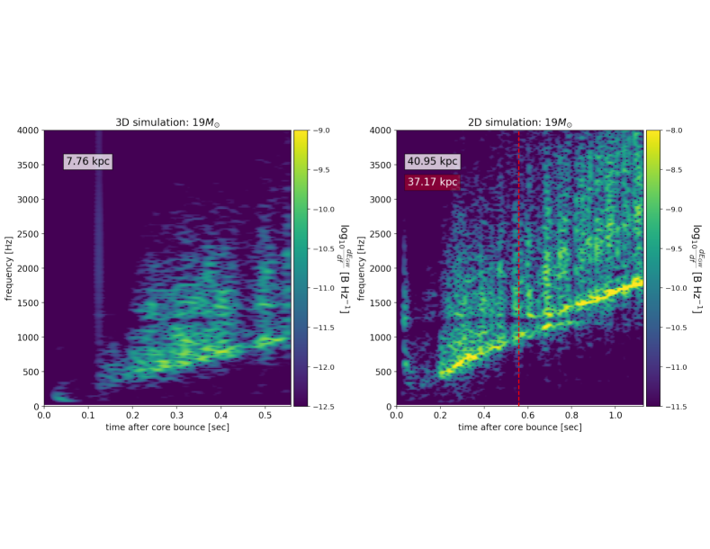
Figure 1: Spectrograms of gravitational-wave waveforms from 3D (left column) and 2D (right column) simulations of $19M_{\odot}$ progenitor. The number on the top left corner each plot with white background is the distance for which these GW signals have an optimal SNR of 8. For the 2D simulations, we recalculate this distance (shown on red background) by truncating the waveform at the end-time of the corresponding 3D simulation. The red vertical dashed line shows the truncation time.

ZAMS Mass	Optimal distance (kpc)			Normalized $\sigma^{2}$ (10Hz-450Hz)		Normalized $\sigma^{2}$ (450Hz-2000Hz)
	3D	2D	2D truncated	3D	2D	3D	2D
$9M_{\odot}$	$2.43$	$15.51$	$15.46$	$0.342$	$0.232$	$0.658$	$0.767$
$11M_{\odot}$	$5.87$	$31.96$	$26.68$	$0.154$	$0.058$	$0.845$	$0.941$
$11M_{\odot}$ (w/o MB)	$5.99$	$28.78$	$26.04$	$0.131$	$0.099$	$0.869$	$0.9$
$19M_{\odot}$ (w/o MB)	$7.75$	$40.61$	$37.18$	$0.120$	$0.074$	$0.880$	$0.925$
$25M_{\odot}$	$13.35$	$48.26$	$40.09$	$0.12$	$0.069$	$0.88$	$0.931$
$60M_{\odot}$	$9.63$	$48.79$	$36.30$	$0.211$	$0.065$	$0.790$	$0.935$

Table 2: The optimal distances for aLIGO and $\sigma^{2}$ for a flat PSD in the frequency bandwidths 10Hz - 450Hz and 450Hz - 2000Hz for waveforms.

We calculate the optimal distance for each of these waveforms, as defined below finn1993observing :

$$d_{opt}=\frac{\sigma}{\rho^{*}}=\frac{1}{\rho^{*}}\left[2\int_{f_{\text{low}}}^{f_{\text{high}}}df\frac{\tilde{h}(f)\tilde{h}^{*}(f)}{S_{h}(f)}\right]^{\frac{1}{2}}$$ (1)

where $S_{h}(f)$ is the power spectral density (PSD) of the detector, $\rho^{*}=8$ is the optimal signal-to-noise ratio (SNR) and the limits over the integral are defined by $f_{\text{low}}$ and $f_{\text{high}}$. We set the lower frequency cutoff, $f_{\text{low}}=10$ Hz and use aLIGOZeroDetHighPower lalsuite as PSD for aLIGO to compute the optimal distances for all the waveforms, which are shown in Table 2. For aLIGO, the average distances for waveforms from 3D simulations are $\sim 8$ kpc, while the average distances for corresponding 2D numerical simulations are $\sim 35.5$ kpc. The 3D simulations have shorter times with respect to the 2D simulations, so we truncate the 2D simulations at the same corresponding times to compare the optimal distances. In doing so, the average optimal distance for the waveforms from the 2D simulations is $\sim 30$ kpc. We find that the 2D waveforms are, on an average, $\sim 4$ times louder than the 3D waveforms. Therefore, we will only use the waveforms from 3D simulations to tune the third generation detectors for CCSN and calculate ranges.

Table 2 also shows the optimal signal-to-noise (SNR) $\sigma^{2}$ of the waveforms in two frequency bandwidths : 10Hz - 450Hz and 450Hz - 2000Hz. These $\sigma^{2}$ values have been calculated using a flat PSD (see section §V), so that we can infer the distribution of the frequency content of the waveforms without being biased by the noise curves of any detector. We can verify from the spectrograms that almost all of the frequency content is below $2000$ Hz. We find that the ratio of $\sigma^{2}$ in the range 10Hz - 450Hz to that in range 450Hz - 2000Hz is $\sim 0.2$ for 3D simulations while for 2D simulations it is $\sim 0.1$. This implies that $\sim 80\%$ of the content of the waveforms is in the frequency range 450Hz - 2000Hz. This is crucial since in Secs §III and §IV, we tune the detector parameters to increase the sensitivity in this frequency range.

In section §III, we define a phenomenological CCSN waveform which is derived from the 3D numerical waveforms. We maximize the range of the phenomenological supernovae waveform (see Fig. 2) with a third-generation Cosmic-Explorer-like detector. We use GWINC to estimate the noise floor for different detector parameters gwinc . The maximized range achieved can then be translated into the corresponding event rate of CCSN, as summarized in table 1 (assuming a 100$\%$ detector duty-cycle).

We use the waveforms from 2019ApJ…876L…9R to compare the ranges of different waveforms of CCSN using the Einstein Telescope (ET), the Cosmic Explorer (CE) and the Supernovae-Optimized detector (SN-Opt). In section V, we invert the problem to calculate the strain requirements of a hypothetical detector to achieve an event rate of the order of one in two years or in the terms of distances – has a range of the order of 10 Mpc for gravitational-wave signals from CCSN. Lastly, we consider in section §V detector configurations beyond the third-generation detectors (Hypothetical) and find the ranges for different numerical waveforms of CCSN.

III Defining a Representative Supernovae Gravitational-Wave Waveform

To maximize the detectable range for CCSN in a given detector configuration, we need a reference CCSN waveform that captures the broad features of supernovae waveform. The reference waveform must have the strain amplitude and spectral features similar to any supernovae waveform. We use the waveforms from the 3D simulations of core-collapse burrows2019three ; 2019ApJ…876L…9R to generate a phenomenological model that captures the broad range of features of core-collapse supernovae waveform. We generate the phenomenological waveform to average out the power emission features from different numerical waveforms so that features in any one of the waveforms do not affect the results of the study. Thereby, the phenomenological waveform provides a model-independent approach.

We construct the phenomenological waveform by a sum of sine-Gaussian bursts. A sine-Gaussian can be defined with three parameters, the central frequency $f_{o}$, the quality factor or the sharpness of the peak $Q$ and the amplitude scale $h_{o}$. The frequency domain representation of a sine-Gaussian can be expressed with these parameters as

$$\tilde{s}(f)=\frac{h_{o}}{4\sqrt{\pi}}\frac{Q}{f_{o}}e^{-\frac{(f-f_{o})^{2}Q^{2}}{4f^{2}}}$$ (2)

The different frequencies are used to model different spectral features of the core-collapse waveform. We choose central frequencies $f_{o}^{i}$ for sine-Gaussian using the numerical waveforms from 3D simulations of core-collapse. We choose, by hand, five distinct central frequencies $f_{o}^{i}$ which correspond to peak emission in the numerical waveforms. We limit ourselves to five distinct values of frequencies in order to avoid over-fitting the sine-Gaussian phenomenological waveform to the numerical waveforms. We note that the supernovae waveforms have emission at higher frequencies but they are much lower in amplitude. Therefore, for the purposes of optimization, we limit ourselves to an upper limit of 2kHz in the phenomenological waveform.

To build the phenomenological waveform, we divide the frequency domain into four bins ranging from – 10 Hz to 250 Hz, 250 Hz to 500 Hz, 500 Hz to 1 kHz and 1 kHz to 2 kHz. For each of the chosen central frequencies $f_{o}^{i}$, the quality factor $Q^{i}$ and the amplitude $h_{o}^{i}$ are chosen so as to minimize the error in the normalized power in the four different bins of frequencies above. The error in the normalized power in each bin is then added in quadrature for different waveforms and is given by

$$\Delta e=\sqrt{\frac{1}{N-1}\sum_{i}^{N}(\mathrm{Model}_{f_{low}}^{f_{high}}-\mathrm{NR}_{f_{low}}^{f_{high}})^{2}}$$ (3)

This approach gives us a simple but robust gravitational waveform, free from the parameter degeneracies but capturing the features of gravitational wave radiation from CCSN. We will use this to perform optimization and maximize the range for this waveform and thus for CCSN. The errors in the different frequency bins ranging from 10Hz to 250Hz, 250Hz to 500Hz, 500Hz to 1kHz and 1kHz to 2kHz is 3$\%$, 9$\%$, 2$\%$ and 19$\%$ respectively. The higher error in the last frequency bin is by the construction of the phenomenological waveform and is added to incorporate the features persistent in the 2D waveforms which show higher emissions in this frequency range discussed in section §II. Fig. 2 shows the phenomenological waveform constructed. We incorporate this waveform as a reference supernovae signal within GWINC gwinc . The ranges, horizon, and reach for the phenomenological waveform can then be calculated by solving for distance $D$ which would rescale the waveform in equation 2 as $1/\mathrm{D}$.

In each of the subsequent sections, we go back to each of the numerical waveforms and recompute the ranges achieved with all the different detector designs considered in our study.

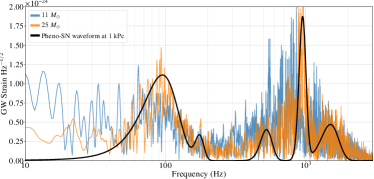
Figure 2: The figure shows the phenomenological waveform used as a representative for gravitational wave emission from CCSN. The waveform is constructed by using five sine-Gaussian bursts with different central frequencies $f_{o}=$ 95, 175, 525, 950 and 1500 Hz. The quality factor and the amplitude at each central frequency are then derived by minimizing the normalized power emitted in four different bins of frequency from 10 Hz to 250 Hz, 250 Hz to 500 Hz, 500 Hz to 1000 Hz and 1000 Hz to 2000 Hz. The overall amplitude of the phenomenological waveform is not calculated by the fit and can be rescaled. We are interested in the broad features in frequency in different waveforms which is effectively captured in the phenomenological waveform.

IV Optimizing SN detectability for 3G detectors

We use the phenomenological gravitational-wave waveform for CCSN to explore detector configurations that optimize the Cosmic Explorer detector’s sensitivity to CCSN. To avoid overemphasis on any particular frequency chosen in the phenomenological waveform, we down weight narrow-band configurations during the process of optimization. We also avoid narrow-band designs so that the optimized detector’s sensitivity to BNS is greater then 1 Gpc. We will explore the narrow-band configurations with a different approach discussed in section §IV.3

IV.1 Broadband configuration tuned for Supernovae

Quantum noise is the predominant source of noise which limits the performance of the gravitational-wave detector. Radiation pressure noise limits the detector sensitivity at low frequencies and shot noise limits sensitivity at high frequencies aasi2015advanced ; acernese2014advanced ; buonanno2003quantum . In our study, we use the design parameters of Cosmic Explorer CEdesignpaper as the starting point. For the purposes of optimization, we choose the Cosmic Explorer rather than the Einstein Telescope as the former has a better noise performance at frequencies which are relevant to CCSN. We optimize over the length of the signal recycling cavity ($\mathrm{L}_{src}$) and the transmissivity of the signal recycling mirror ($\mathrm{T}_{srm}$) to maximize the CCSN detection range. The quantum resonant sidebands can be tuned with these parameters and we exploit this behavior for supernovae tuning similar to the approach used by Buonanno et al. BunnChen2004 and Martynov et al. martynov2019exploring .

We also study, the effect of the length of the arm cavity ($\mathrm{L}_{arm}$) on supernovae sensitivity. We use Markov Chain Monte Carlo sampling hastings1970monte and particle swarm optimization PSO1995 to search the parameter space and maximize the range for the phenomenological waveform for a broadband detector. During the process of maximizing the range, we down-weight the narrow-band configurations with two constraints for sample points. First, the reflectivity of the signal recycling cavity $\mathrm{T}_{srm}>$ 0.01. Second, the given detector configuration must have a optimal distance for binary neutron stars systems ($m_{1}=m_{2}=1.4~{}M_{\odot}$ and $s_{1z}=s_{2z}=0$) to be greater than 1 Gpc. By doing so, we ensure that the detector’s sensitivity is not lost for compact binaries.

The strain sensitivity improves as the square root of the arm length of the detector as long as the gravitational-wave frequency ($\Omega$) is much less than the free spectral range ($\mathrm{f}_{FSR}$) of the Fabry-Perot cavity. The strain sensitivity of the detector does not always improve by scaling the detector as other fundamental sources of noise also change by scaling the length of the detector dwyer2015gravitational . As the gravitational wave spectrum of supernovae has some power in a few kilohertz range, we allow the arm length to vary independently similar to the analysis by Miao2018 ; martynov2019exploring . Our simulations indicated the optimal length to be close to 40 km, the upper bound value allowed for the length parameter. As a result, we set the length of the arm cavity to 40 km. For a 40 km arm length, the $\mathrm{f}_{FSR}$ is 3750 Hz. The sensitivity of the detector is limited by the $\mathrm{f}_{FSR}$, any further increase in the length of the arms will reduce the $\mathrm{f}_{FSR}$, resulting in the loss in sensitivity to CCSN, where the gravitational wave spectrum persists up to a few kilohertz.

The optimal supernovae zero-detuned detector’s noise budget is shown in Fig. 3. We find a longer signal recycling with a length of 180 m compared to 55m for Cosmic Explorer along with a transmissivity of the signal recycling cavity changed to 0.015 improved the detector’s sensitivity by improving the quantum noise floor at higher frequencies. The loss in sensitivity around 3 kHz is due to the FSR of the arm cavity. The dip at 4 kHz corresponds to the pole of the signal recycling cavity.

We also consider the effects of detuning the signal recycling cavity. We find detuning the signal recycling cavity with active compensation with the squeezing phase can be used to actively tune the third generation detectors in narrow bins of frequency without losing 15 dB of squeezing. It has been proposed that detuning the ground-based detectors can be useful in testing the general theory of relativity tso2018optimizing with a joint operation with LISA danzmann1996lisa . We will consider the applicability of these configurations to see if they provide any improvements for CCSN in section §IV.2.

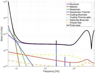
Figure 3: The figure summarizes the noise budget of the supernovae-optimized detector for a gravitational-wave signal with a 45 degrees tilt with respect to the arm cavities schilling1997angular . Over the broad range of frequencies of interest, 500 Hz to 1500 Hz, the sensitivity is limited by quantum noise. The dip in sensitivity at 4 kHz corresponds to the pole of the signal recycling cavity.

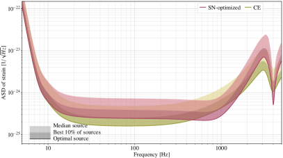
Figure 4: The figure summarizes the sky-averaged and orientation-averaged power spectral density of Cosmic Explorer and supernovae-tuned detector essick2017frequency . We see that the Cosmic Explorer has a better noise floor from 10 Hz to 450 Hz. The supernovae-tuned detector has improved sensitivity over the range from 450 Hz to 1600 Hz. The numerical waveforms of CCSN suggest that a significant amount of power is emitted in this range. The optimization for CCSN improves the range from 70 kpc to 95 kpc for CCSN. However, this range improvement does not add any new galaxies. Therefore, the event rate does not change with the improved sensitivity and we are limited to sources within our galaxy.

The optimization over the length of the signal recycling cavity and the transitivity of the signal recycling mirror to maximize the supernovae range with the phenomenological waveform in Fig. 2 leads to an improvement of approximately 30$\%$ in the range of CCSN as compared to the Cosmic Explorer design. However, extending the range from a 70 kpc to 95 kpc does not add any galaxies in our local universe. The optimized supernovae detector does not increase the detection rate as compared to the Cosmic Explorer. For the sources at a fixed distance, this corresponds to approximately 25$\%$ improvement in SNR.

The Fig. 4 compares the broadband configuration of a zero detuned 40 km detector optimized for CCSN signals with the design of the Cosmic Explorer, both configurations have a 15dB squeezing. We improve on the sensitivity in the frequency range from 450 Hz to 1550 Hz at the cost of a loss in sensitivity from 10 Hz to 450 Hz. This results in a 15$\%$ loss in range for BNS. However, it still provides higher sensitivity for the post-merger signals based on the predicted frequencies of interest for post-merger oscillations abbott2017gw170817 ; bauswein2019identifying ; bose2018neutron ; takami2014constraining . The table  3 summarizes the parameters and their corresponding ranges towards different gravitational-wave sources. One advantage offered by the supernovae optimized configuration is robustness. Without any squeezing, the supernovae optimized detector has a range extending to the LMC, whereas the range of the phenomenological SN waveform with Cosmic Explorer without squeezing is 32 kpc.

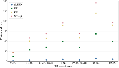
Figure 5: The figure summarizes the distance of the 3D waveforms for different second and third-generation gravitational wave detectors. We see for second-generation advanced LIGO detector that the optimal distances for the 3D numerical waveforms are limited to  10kpc. The optimal distance is so small enough that we are not sensitive to all the galactic supernovae. All the third-generation detectors have optimal distance such that each detector is sensitive enough to detect gravitational waves from galactic CCSN. However, as evident from the plot above, for a source at a fixed distance, the ET will have the lower SNR as compared to Cosmic Explorer. The supernovae-optimized detector provides approximately a 25$\%$ improvement in the SNR as compared to Cosmic Explorer.

Next, we use the noise curves of aLIGO, Cosmic Explorer, Einstein Telescope and Supernovae optimized detector configurations to compute the ranges for the 3D waveforms As stated earlier, the 3D waveforms are representative of astrophysically abundant stars which are not rapidly rotating and the corresponding gravitational wave strain emitted is small. Figure 5 summarizes the ranges of different waveforms based on their ZAMS mass. We see that the sensitivity of the third-generation of gravitational-wave detectors to CCSN is limited to sources within our galaxy. From the event rates of CCSN summarized in table 1, we find the corresponding event rate of observation of gravitational waves from CCSN (assuming a 100 $\%$ detector duty-cycle) is approximately one in fifty years.

IV.2 Detuning a large signal recycling cavity for narrow-band configurations

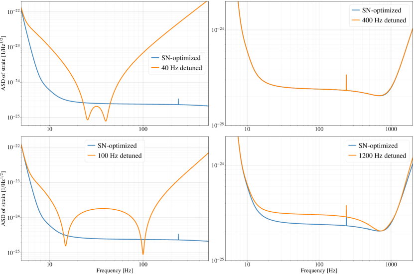
Figure 6: We explore the possibility of detuning the signal recycling cavity to improve the sensitivity towards CCSN. We find that detuning can be used to improve sensitivity in narrow bins of frequency below 400 Hz. This could, therefore, be used to study the ring-down modes of binary black-holes systems in collaboration with eLISA tso2018optimizing . However, for improvements to the range of CCSN, this technique isn’t useful.

A significant GW signal from CCSN lies in the frequency band from 500 Hz to 1500 Hz. The power emitted at different frequencies may vary depending on the astrophysical features of the star - mass, rotation speed, equation of state, etc Burrows2007_RapidRot ; burrows2019three ; Radice_2019_Characterstics ; Heger_2005 .

In this section, we do not change the detector parameters’ such as the transitivity or the length of the signal recycling cavity. This is because these parameters cannot be changed once the detector design is laid out. However, one can detune the signal recycling cavity to maximize sensitivity in a narrow band of frequencies hild2007demonstration ; ward2010length . This response from detuning the signal recycling cavity arises from the two sidebands resonances in quantum noise BunnChen2004 ; buonanno2003quantum . We consider the detuning of the signal recycling cavity at different frequencies.

We maintain the frequency dependent squeezing of 15 dB. We achieve 15 dB squeezing in a detuned signal recycling cavity without losing the injected squeezing by actively changing the squeezing angle in accordance with the amount of detuning. Thus, detuning the signal recycling cavity along with actively changing the squeezing angle can be used to switch from a broadband zero-detuned detector to a narrow band detector with greater sensitivity for some frequencies determined by the magnitude of detuning. We perform another tier of optimization in which we actively vary the amount of detuning and the squeezing angle. We limit the amount of detuning in the range from $-\pi/5$ to $\pi/5$ and the squeezing phase is tuned in between $-\pi$ to $\pi$. To optimize the detector response at frequencies of 40 Hz, 100 Hz, 400 Hz and 1200 Hz, we inject a sine-Gaussian at each frequency and then maximize the range for this injected signal by varying only the detuning and squeezing angle for the supernovae optimized detector.

We find that detuning the signal can improve the sensitivity of the detector in narrow bins of frequency below 400 Hz. We do not achieve improvements in sensitivity at higher frequencies therefore, we do not improve the range for different models by detuning the detector. There are no improvements in the optimal SNR values for a source at a fixed distance. In summary, detuning the signal recycling cavity is not useful for improving the Cosmic-Explorer-like detector’s sensitivity to CCSN. Instead, detuning the signal recycling cavity at higher frequency degrades the sensitivity of the broadband supernovae-optimized detector. The corresponding results of detuning the signal recycling cavity are summarized in Fig. 6.

IV.3 Narrow-band Configurations tuned for Supernovae

The parameters of the broadband supernovae-optimized detector were computed in section §IV.1 with two constraints. We will in this section relax those constraints and consider narrow-band detector configurations to maximize the range for CCSN. The phenomenological waveform we developed cannot be used for narrow-band optimization as the fit was performed to match the power of the 3D waveforms over a broad frequency bandwidth. Therefore, we find narrow-band configurations using a different technique.

The length of the signal recycling cavity can be changed to tune the resonant frequency of arising from the coupling of the signal recycling cavity with the arms of the interferometer meers1988recycling ; BunnChen2004 . The bandwidth of the resonance at a frequency $\omega_{r}$ is given by

$$B=\frac{\mathrm{cT}_{srm}}{4\mathrm{L}_{src}}$$ (4)

where $\mathrm{T}_{srm}$ is the transmissivity of the signal recycling mirror and $\mathrm{L}_{src}$ is the length of the signal recycling cavity. We choose the length of the signal recycling cavity at 150m, 300m and 750m are such that the resonant frequency $\omega_{r}$ is at 1000 Hz, 750 Hz and 500 Hz respectively. The equation 4 is then inverted for bandwidth ranging from 250 Hz to 1600 Hz and the corresponding values of the transmissivity of the signal recycling mirror are calculated.

We find that a narrow-bandwidth of 250 Hz significantly affects the sensitivity of the detector towards CCSN. This is expected as we have stated earlier that the frequency spectrum of gravitational wave emission from CCSN is broadband. The range improvements achieved by narrow-band detectors at 500 Hz, 750 Hz and 1000 Hz with a bandwidth of 250 Hz are also varying from waveform to waveform and therefore is not model independent 7. When the bandwidth is increased to 1600 Hz the range improves for the 750 Hz narrow-band detector for some of the waveforms as shown in Fig. 7. The $\mathrm{L}_{src}$ = 300m and $\mathrm{T}_{srm}$ = 0.0064 give this narrow-band detector configuration. The mean improvement in optimal SNR with the 750 Hz narrow-band and 1600 Hz bandwidth detector is approximately 10 $\%$ with respect to the supernovae optimized broadband detector. However, we caution that the improvement from narrow banding is not the same across all the 3D numerical waveforms. Moreover, this comes at the cost of significant loss of sensitivity below 400 Hz and above 1100 Hz. The range for BNS drops to 3 Gpc (z=0.9) compared to 3.7 Gpc (z=1.1) for supernovae-optimized Cosmic Explorer and 4.3 Gpc (z=1.4) with respect to the Cosmic Explorer.

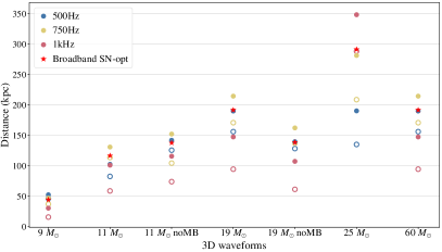
Figure 7: The figure summarizes the optimal distance of the different 3D waveforms for narrow-band detectors at frequencies 500 Hz, 750 Hz and 1000 Hz. The hollow circles denote the narrow-band detectors with a bandwidth of 250 Hz while the filled circles denote the bandwidth of 1600 Hz. The optimal distances from the broadband supernovae-optimized detector are represented as stars. We see tighter narrow-banding with a bandwidth of 250 Hz degrades the performance of the detector. The wider bandwidth of 1600 Hz around the 750 Hz narrow-band detector improves the optimal distances for most of the numerical waveforms.

V Challenges in building a CCSN Detector to achieve Higher Event rates

In section §IV.1, we find an optimized third-generation broadband gravitational wave detector for a CCSN signal has the range only to a few hundred kilo-parsec for the 3D numerical waveforms of CCSN.

We now address the question of what are the strain requirements for a gravitational-wave detector to be able to detect CCSN with an event rate of 0.5 per year. From the table 1, we see that this “Hypothetical CCSN detector” must have a range of $\mathcal{O}$(10 Mpc) for CCSN to achieve an event rate of 0.5 per year. Moreover, a single detector, we need a signal to noise ratio (SNR) of 8 to define the detection of a signal against the background. Using the two constraints above we can calculate the minimum strain sensitivity required to achieve an event rate of 0.5 per year for the waveforms from 3D numerical simulations. The optimal distance for the numerical waveforms can be calculated by equation 1. The limits over the integral are defined by $f_{low}$ and $f_{high}$. To find the strain requirements for the different waveforms we assume a flat PSD over a broadband range of frequency ranging from $f_{low}$ and $f_{high}$. We consider two scenarios which are summarized in the figures 8. First, we vary the upper limit of the frequency integrated – $f_{High}$ with the lower limit of integration is held constant at 10 Hz. The second scenario where the upper limit of integration is constant at 2 kHz and we vary the lower frequency limit $f_{low}$. We find the minimum strain sensitivity required for the gravitational-wave detector to detect the CCSN with an event rate of 0.5 per year is $3\times 10^{-27}~{}\mathrm{Hz}^{-1/2}$ over a frequency range of 100 Hz to 1500 Hz.

Thus, we need a detector with sensitivity approximately a hundred times better than the Cosmic Explorer design to detect CCSN with an event rate of 0.5 per year. In the next section §V, we will summarize the noise limitations of the third generation detectors and consider design parameters for gravitational-wave detectors beyond the scope of the third-generation to determine the technological hurdles to overcome in order to ever observe gravitational signals from CCSN more frequently.

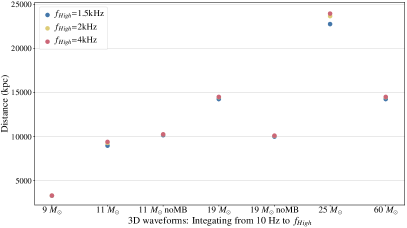
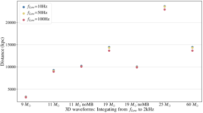
Figure 8: Considering toy detector with a flat PSD of 3$\times 10^{-27}~{}Hz^{-1/2}$ in range 10 Hz to $f_{High}$ (above) and $f_{low}$ to 2 kHz (below), the figure summarizes the range with the corresponding sensitivity and numerical waveform CCSN corresponding to their ZAMS mass. We see a broadband detector with a strain sensitivity of 3$\times 10^{-27}~{}Hz^{-1/2}$ from 200 Hz to 1.5 kHz is desired to achieve the ranges that would correspond to an observed event rate of one per year for gravitational-waves from CCSN.

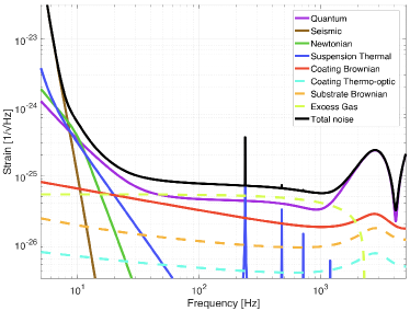
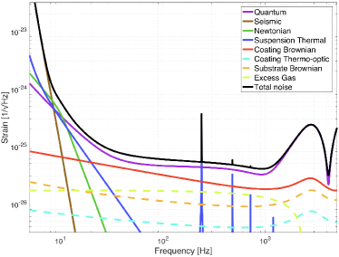
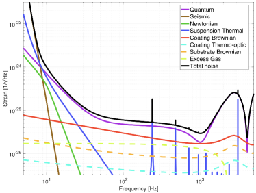
Figure 9: The figure above summarizes the noise budgets for the Hypothetical detector configurations. We see from the figure on the top that the detector’s sensitivity is limited by residual gas noise. Therefore, we reduce the residual gas pressure by a factor of ten from CE design. The plot in the middle and bottom plots show optimization results without changing the transmittance of the power recycling cavity and with active changes in the transmittance of the power recycling cavity. Thereby, changing the gain of the power recycling cavity and the finesse of the detector. We will refer to the two detector configurations as Hypothetical-1 and Hypothetical-2 respectively.

It is evident from Fig. 3 that the sensitivity is limited by the quantum noise in the broad range of frequencies. The standard quantum noise limit is dependent primarily on the length of the arm cavities, the test masses and the power of the input laser braginsky1996quantum . The length of the arm cavities cannot be increased any further as the $\mathrm{f}_{FSR}$ would significantly affect the performance of the detector at the frequencies of interest. As a result, we set the length of the Hypothetical detectors to 40 kms. Increasing the power of the input laser is the one possibility to reduce quantum noise. We assume an input laser power of 500W. At high frequencies, the quantum noise in the detector manifests itself as shot noise and is limited by photon number arriving at the photo-detector. To see the best we can achieve, we set the photo-detection efficiency of the photo-detector in Hypothetical to 1 (from 0.96 for CE design). For the same reason, we also set the optical and squeezing injection losses in the detector to zero.

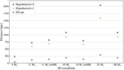
Figure 10: The plot shows with extreme technological upgrades to the third-generation detectors discussed in section §V, we optimal distances for the CCSN is limited to 1Mpc. The event rate for the observation of gravitational waves from CCSN is still low but improves to one in twenty years.

The coating thermal noise and the residual gas noise are the next limiting factor in the system. We reduce the substrate absorption by an order of magnitude from CE design. Lastly, as the frequency range of interest is from 100Hz we can sacrifice the sensitivity at lower frequencies. Thus, we can reduce the masses of the mirrors as we are interested in improving the shot noise characteristics of the detector, at the cost of higher radiation pressure noise. In this setup we optimize over the length of the signal recycling cavity $\mathrm{L}_{src}$, the transmissivity of the signal recycling mirror $\mathrm{T}_{srm}$, the transmissivity of the input test mass $\mathrm{T}_{itm}$ and the scale mass parameter to change the masses of the mirror. The optimization over these parameters is aimed at maximizing the range for the representative supernovae waveform, we will reference this optimized detector as Hypothetical-1.

The quantum noise limit in a dual-recycled Fabry-Perot interferometer also depends on the gain of the power recycling cavity BunnChen2004 ; buonanno2003quantum . We will in another independent optimization also tune the transmissivity of the power recycling mirror $\mathrm{T}_{prm}$ along with the above parameters. We define this supernovae-optimized detector as Hypothetical-2. The table 3 summarizes the optimal parameters of different detectors. Fig. 9 shows the noise budget of the Supernovae optimized Hypothetical detectors. We see that the residual is the limiting source of the noise. Removing the residual gas noise improves the noise floor of the detector by a factor of two in the wide range of frequencies of interest, see Fig. 9. After removing the residual gas noise, we are limited in sensitivity by quantum noise over the broad range of frequencies.

The strain sensitivity achieved after removing the residual gas noise is $5\times 10^{-26}\mathrm{Hz}^{-1/2}$. The improvements in photo-detection efficiency, the input laser power, substrate coatings and minimization of optical losses are not sufficient to achieve a strain sensitivity of the order of $3\times 10^{-27}~{}\mathrm{Hz}^{-1/2}$ required to detect CCSN with an event rate of one in two years (see section §V).

Lastly, we revisit the numerical waveforms of core-collapse supernovae to see the ranges achieved by the Hypothetical supernovae-optimized detector designs. We find for the 3D waveforms from numerical simulations have a mean distance of 800 kpc, see Fig. 10. Thus, with beyond the third generation detector designs, we would be able to observe core-collapse supernovae from Andromeda. The corresponding event rate is of the order of one in twenty years. The event rate calculation assumes a 100$\%$ duty cycle of the detector. The observation rate of gravitational waves from CCSN is low even for gravitational-wave detectors beyond the scope of the third-generation detectors.

Parameters	aLIGO	Cosmic Explorer-2	SN Optimized	Hypothetical-1	Hypothetical-2
Input Power	125W	220W	220W	500W	500W
SRM transmission	0.325	0.04	0.015	0.0030	0.0122
ITM transmission	0.014	0.014	0.014	0.0036	0.0269
PRM transmission	0.030	0.030	0.030	0.030	0.0011
$\mathrm{L}_{src}$	55m	55m	175m	30m	260m
Finesse	446.25	447.52	447.52	1745.33	233.33
Power Recycling Factor	40.66	65.32	65.32	94.25	1300.09
Arm power	712.43 kW	2025.70 kW	2025.70 kW	26.06 MW	47.61 MW
Thermal load on ITM	0.386 W	1.150 W	1.150 W	13.094 W	24.180 W
Thermal load on BS	0.051 W	0.253 W	0.253 W	0.008 W	0.080 W
BNS range	173.00 Mpc	4.29 Gpc	3.67 Gpc	5.32 Gpc	5.09 Gpc
BNS horizon	394.83 Mpc	11.05 Gpc	9.49 Gpc	12.97 Gpc	12.53 Gpc
BNS reach	246.06 Mpc	8.54 Gpc	6.90 Gpc	11.56 Gpc	10.80 Gpc
BBH range	1.61 Gpc	6.13 Gpc	6.10 Gpc	6.15 Gpc	6.09 Gpc
BBH horizon	3.81 Gpc	11.86 Gpc	11.85 Gpc	11.85 Gpc	11.70 Gpc
BBH reach	2.54 Gpc	11.73 Gpc	11.73 Gpc	11.72 Gpc	11.52 Gpc
Supernovae range	4.34 kpc	71.95 kpc	94.24 kpc	540.53 kpc	716.03 kpc
Supernovae horizon	9.84 kpc	163.08 kpc	213.61 kpc	1225.22 kpc	1623.06 kpc
Supernovae reach	6.10 kpc	101.04 kpc	132.35 kpc	759.15 kpc	1005.65 kpc
Stochastic Omega	2.36e-09	1.82e-13	2.77e-13	1.1e-13	2.58e-13

Table 3: Summary of All Detectors

VI Conclusion

We have shown that it is possible to tune a Cosmic Explorer detector to increase the range to CCSN by approximately 25$\%$. This range improvement does not translate to increase in detection rate due to the inhomogeneity of the local universe. Therefore, even optimized third-generation gravitational-wave detectors will be limited to CCSN sources within our galaxy and the Magellanic Clouds. Assuming the detectors have a duty-cycle of 100$\%$ the corresponding event rate of CCSN is one in fifty years. Incorporating the detector downtime and duty-cycle would further decrease the event rate of observed gravitational-wave signals from CCSN.

However, if such an event were to occur, the broadband supernovae-optimized detector would improve the SNR by of sources by 25$\%$. This improvement would facilitate help understand the properties of the progenitor star in the rare event of CCSN observation. The supernovae-optimized detector has a slightly reduced sensitivity to the inspiral of neutron stars, but the high-frequency improvements would benefit the study of post-merger signatures and the late-time behavior of the inspiral.

We find that a gravitational-wave detector would require a strain sensitivity of the order of 3$\times$10^-27 $\mathrm{Hz}^{-1/2}$, over a frequency range from 100 Hz to 1500 Hz in order to guarantee a high rate of CCSN detection. At this strain sensitivity, as per the current estimates of the BNS background, the stochastic background from BNS mergers would contribute as the fundamental sources of noise abbott2018gw170817 . This along with technological challenges discussed in section §V poses significant hurdles in achieving an event rate of one per year for the observation of gravitational-waves from CCSN based on the present models and knowledge of gravitational-wave emission from CCSN. The technological requirements for these upgrades are beyond the requirements for the third-generation detector. With drastic improvements of an input laser power of 500 W and a photo-detection efficiency of 1, an order of magnitude improvement in the residual gas noise and coating noise from the Cosmic Explorer design, and assuming minimal optical losses in Hypothetical detectors. We find that after optimizing these detector configurations to maximize for the supernovae range the range extends to Andromeda for some of the CCSN numerical waveforms. The event rate achieved with such a hypothetical detector is one in twenty years.

VII Acknowledgements

We would like to thank Evan Hall and Joshua Smith for their help with GWINC. We thank Geoffrey Lovelace and Christopher Wipf for helpful discussions in regards with the astrophysical implications of the results. VS, SB, DAB, and CA thank the National Science Foundation for support through award PHY-1836702. AB, DR, and DV acknowledge support from the U.S. Department of Energy Office of Science and the Office of Advanced Scientific Computing Research via the Scientific Discovery through Advanced Computing (SciDAC4) program and Grant DE-SC0018297 (subaward 00009650), the U.S. NSF under Grants AST-1714267 and PHY-1144374, the DOE/ASCR INCITE program under Contract DE-AC02-06CH11357, a Blue Waters PRAC (under OCI-0725070, OAC-1809073, and ACI-1238993), and the National Energy Research Scientific Computing Center (NERSC) under contract DE-AC03-76SF00098. DAB thanks NSF award PHY-1748958 to the Kavli Institute for Theoretical Physics for support.

References

- (1) Junaid Aasi, BP Abbott, Richard Abbott, Thomas Abbott, MR Abernathy, Kendall Ackley, Carl Adams, Thomas Adams, Paolo Addesso, RX Adhikari, et al. Advanced ligo. Classical and quantum gravity, 32(7):074001, 2015.
- (2) F Acernese, M Agathos, K Agatsuma, D Aisa, N Allemandou, A Allocca, J Amarni, P Astone, G Balestri, G Ballardin, et al. Advanced virgo: a second-generation interferometric gravitational wave detector. Classical and Quantum Gravity, 32(2):024001, 2014.
- (3) Benjamin P Abbott, Richard Abbott, TD Abbott, MR Abernathy, Fausto Acernese, Kendall Ackley, Carl Adams, Thomas Adams, Paolo Addesso, RX Adhikari, et al. Observation of gravitational waves from a binary black hole merger. Physical review letters, 116(6):061102, 2016.
- (4) Benjamin P Abbott, R Abbott, TD Abbott, MR Abernathy, F Acernese, K Ackley, C Adams, T Adams, P Addesso, RX Adhikari, et al. Gw151226: Observation of gravitational waves from a 22-solar-mass binary black hole coalescence. Physical review letters, 116(24):241103, 2016.
- (5) Benjamin P Abbott, Rich Abbott, TD Abbott, Fausto Acernese, Kendall Ackley, Carl Adams, Thomas Adams, Paolo Addesso, RX Adhikari, VB Adya, et al. Gw170817: observation of gravitational waves from a binary neutron star inspiral. Physical Review Letters, 119(16):161101, 2017.
- (6) The LIGO Scientific Collaboration, the Virgo Collaboration, B.~P. Abbott, R Abbott, T.~D. Abbott, S Abraham, F Acernese, K Ackley, C Adams, R.~X. Adhikari, and Et al. GWTC-1: A Gravitational-Wave Transient Catalog of Compact Binary Mergers Observed by LIGO and Virgo during the First and Second Observing Runs. arXiv e-prints, nov 2018.
- (7) Tejaswi Venumadhav, Barak Zackay, Javier Roulet, Liang Dai, and Matias Zaldarriaga. New binary black hole mergers in the second observing run of advanced ligo and advanced virgo. arXiv preprint arXiv:1904.07214, 2019.
- (8) Alexander H Nitz, Collin Capano, Alex B Nielsen, Steven Reyes, Rebecca White, Duncan A Brown, and Badri Krishnan. 1-ogc: The first open gravitational-wave catalog of binary mergers from analysis of public advanced ligo data. The Astrophysical Journal, 872(2):195, 2019.
- (9) Alejandro Torres-Forné, Pablo Cerdá-Durán, Martin Obergaulinger, Bernhard Muller, and José A Font. Universal relations for gravitational-wave asteroseismology of proto-neutron stars. arXiv preprint arXiv:1902.10048, 2019.
- (10) Sherwood Richers, Christian D Ott, Ernazar Abdikamalov, Evan O’Connor, and Chris Sullivan. Equation of state effects on gravitational waves from rotating core collapse. Physical Review D, 95(6):063019, 2017.
- (11) Ernazar Abdikamalov, Sarah Gossan, Alexandra M DeMaio, and Christian D Ott. Measuring the angular momentum distribution in core-collapse supernova progenitors with gravitational waves. Physical Review D, 90(4):044001, 2014.
- (12) Benjamin P Abbott, Richard Abbott, TD Abbott, MR Abernathy, F Acernese, K Ackley, C Adams, T Adams, P Addesso, RX Adhikari, et al. First targeted search for gravitational-wave bursts from core-collapse supernovae in data of first-generation laser interferometer detectors. Physical Review D, 94(10):102001, 2016.
- (13) BP Abbott, R Abbott, TD Abbott, S Abraham, F Acernese, K Ackley, C Adams, RX Adhikari, VB Adya, C Affeldt, et al. All-sky search for short gravitational-wave bursts in the second advanced ligo and advanced virgo run. arXiv preprint arXiv:1905.03457, 2019.
- (14) S E Gossan, P Sutton, A Stuver, M Zanolin, K Gill, and C D Ott. Observing gravitational waves from core-collapse supernovae in the advanced detector era. Phys. Rev. D, 93(4):42002, feb 2016.
- (15) Weidong Li, Jesse Leaman, Ryan Chornock, Alexei V Filippenko, Dovi Poznanski, Mohan Ganeshalingam, Xiaofeng Wang, Maryam Modjaz, Saurabh Jha, Ryan J Foley, and Others. Nearby supernova rates from the Lick Observatory Supernova Search–II. The observed luminosity functions and fractions of supernovae in a complete sample. Monthly Notices of the Royal Astronomical Society, 412(3):1441–1472, 2011.
- (16) Weidong Li, Ryan Chornock, Jesse Leaman, Alexei V Filippenko, Dovi Poznanski, Xiaofeng Wang, Mohan Ganeshalingam, and Filippo Mannucci. Nearby supernova rates from the Lick Observatory Supernova Search–III. The rate–size relation, and the rates as a function of galaxy Hubble type and colour. Monthly Notices of the Royal Astronomical Society, 412(3):1473–1507, 2011.
- (17) M L Graham, D J Sand, C J Bildfell, C J Pritchet, D Zaritsky, H Hoekstra, D W Just, S Herbert-Fort, S Sivanandam, and R J Foley. The Type II Supernova Rate in z0.1 Galaxy Clusters from the Multi-Epoch Nearby Cluster Survey. The Astrophysical Journal, 753(1):68, jun 2012.
- (18) Lin Xiao and J J Eldridge. Core-collapse supernova rate synthesis within 11 Mpc. Monthly Notices of the Royal Astronomical Society, 452(3):2597–2605, 2015.
- (19) D. Radice, V. Morozova, A. Burrows, D. Vartanyan, and H. Nagakura. Characterizing the Gravitational Wave Signal from Core-collapse Supernovae. The Astrophysical Journal Letters, 876:L9, May 2019.
- (20) J. W. Murphy, C. D. Ott, and A. Burrows. A Model for Gravitational Wave Emission from Neutrino-Driven Core-Collapse Supernovae. The Astrophysical Journal, 707:1173–1190, December 2009.
- (21) V. Morozova, D. Radice, A. Burrows, and D. Vartanyan. The Gravitational Wave Signal from Core-collapse Supernovae. The Astrophysical Journal, 861:10, July 2018.
- (22) T. Kuroda, T. Takiwaki, and K. Kotake. Gravitational wave signatures from low-mode spiral instabilities in rapidly rotating supernova cores. Phys. Rev. D, 89(4):044011, February 2014.
- (23) H. Andresen, B. Müller, E. Müller, and H.-T. Janka. Gravitational wave signals from 3D neutrino hydrodynamics simulations of core-collapse supernovae. Monthly Notices of the Royal Astronomical Society, 468:2032–2051, June 2017.
- (24) K. N. Yakunin, A. Mezzacappa, P. Marronetti, E. J. Lentz, S. W. Bruenn, W. R. Hix, O. E. B. Messer, E. Endeve, J. M. Blondin, and J. A. Harris. The Gravitational Wave Signal of a Core Collapse Supernova Explosion of a 15M Star. ArXiv e-prints, January 2017.
- (25) Takami Kuroda, Kei Kotake, Kazuhiro Hayama, and Tomoya Takiwaki. Correlated Signatures of Gravitational-Wave and Neutrino Emission in Three-Dimensional General-Relativistic Core-Collapse Supernova Simulations. Astrophys. J., 851(1):62, 2017.
- (26) Jade Powell and Bernhard Müller. Gravitational wave emission from 3d explosion models of core-collapse supernovae with low and normal explosion energies. arXiv preprint arXiv:1812.05738, 2018.
- (27) John M Scalo. The stellar initial mass function. Fundamentals of cosmic physics, 11:1–278, 1986.
- (28) Scott M Adams, CS Kochanek, John F Beacom, Mark R Vagins, and KZ Stanek. Observing the next galactic supernova. The Astrophysical Journal, 778(2):164, 2013.
- (29) E Cappellaro, M Turatto, D Yu Tsvetkov, OS Bartunov, C Pollas, R Evans, and M Hamuy. The rate of supernovae from the combined sample of five searches. Astron. Astrophys, 322:431–441, 1997.
- (30) FX Timmes and SE Woosley. Gamma-ray line signals from 26al and 60fe in the galaxies of the local group. The Astrophysical Journal Letters, 481(2):L81, 1997.
- (31) Michael J Pierce, Douglas L Welch, Robert D McClure, Sidney van den Bergh, Renè Racine, and Peter B Stetson. The hubble constant and virgo cluster distance from observations of cepheid variables. Nature, 371(6496):385, 1994.
- (32) GA Tammann, W Loeffler, and A Schroeder. The galactic supernova rate. The Astrophysical Journal Supplement Series, 92:487–493, 1994.
- (33) Massimo Capaccioli, Massimo Della Valle, Mauro D’Onofrio, and Leonida Rosino. Properties of the nova population in m31. The Astronomical Journal, 97:1622–1633, 1989.
- (34) G. A. Tammann, W. Loeffler, and A. Schroeder. The Galactic supernova rate. The Astrophysical Journal Supplement, 92:487–493, June 1994.
- (35) Wendy L Freedman and Barry F Madore. An empirical test for the metallicity sensitivity of the cepheid period-luminosity relation. The Astrophysical Journal, 365:186–194, 1990.
- (36) S Mattila and WPS Meikle. Supernovae in the nuclear regions of starburst galaxies. Monthly Notices of the Royal Astronomical Society, 324(2):325–342, 2001.
- (37) M. T. Botticella, S. J. Smartt, R. C. Kennicutt, E. Cappellaro, M. Sereno, and J. C. Lee. A comparison between star formation rate diagnostics and rate of core collapse supernovae within 11 Mpc. Astronomy and Astrophysics, 537:A132, Jan 2012.
- (38) S Mattila, Tomas Dahlén, Andreas Efstathiou, Erkki Kankare, Jens Melinder, Almudena Alonso-Herrero, MÁ Pérez-Torres, S Ryder, P Väisänen, and Göran Östlin. Core-collapse supernovae missed by optical surveys. The Astrophysical Journal, 756(2):111, 2012.
- (39) Matthew D Kistler, Hasan Yüksel, Shin’ichiro Ando, John F Beacom, and Yoichiro Suzuki. Core-collapse astrophysics with a five-megaton neutrino detector. Physical Review D, 83(12):123008, 2011.
- (40) Sidney van den Bergh and Gustav A Tammann. Galactic and extragalactic supernova rates. Annual Review of Astronomy and Astrophysics, 29(1):363–407, 1991.
- (41) M. Aaron Skinner, Joshua C. Dolence, Adam Burrows, David Radice, and David Vartanyan. FORNAX: A Flexible Code for Multiphysics Astrophysical Simulations. The Astrophysical Journal Supplement Series, 241:7, Mar 2019.
- (42) M Aaron Skinner, Adam Burrows, and Joshua C Dolence. Should one use the ray-by-ray approximation in core-collapse supernova simulations? The Astrophysical Journal, 831(1):81, 2016.
- (43) Tuguldur Sukhbold, T Ertl, SE Woosley, Justin M Brown, and H-T Janka. Core-collapse supernovae from 9 to 120 solar masses based on neutrino-powered explosions. The Astrophysical Journal, 821(1):38, 2016.
- (44) Tuguldur Sukhbold, SE Woosley, and Alexander Heger. A high-resolution study of presupernova core structure. The Astrophysical Journal, 860(2):93, 2018.
- (45) Viktoriya Morozova, David Radice, Adam Burrows, and David Vartanyan. The Gravitational Wave Signal from Core-collapse Supernovae. The Astrophysical Journal, 861(1):10, jun 2018.
- (46) Lee Samuel Finn and David F Chernoff. Observing binary inspiral in gravitational radiation: One interferometer. Physical Review D, 47(6):2198, 1993.
- (47) LIGO Scientific Collaboration. LIGO Algorithm Library - LALSuite. free software (GPL), 2018.
- (48) The LIGO Scientific Collaboration. Gravitational Wave Interferometer Noise Calculator.
- (49) Adam Burrows, David Radice, and David Vartanyan. Three-dimensional supernova explosion simulations of 9-, 10-, 11-, 12-, and 13-M⊙ stars. Monthly Notices of the Royal Astronomical Society, 485(3):3153–3168, 2019.
- (50) Alessandra Buonanno, Yanbei Chen, and Nergis Mavalvala. Quantum noise in laser-interferometer gravitational-wave detectors with a heterodyne readout scheme. Physical Review D, 67(12):122005, 2003.
- (51) Benjamin P Abbott, R Abbott, T D Abbott, M R Abernathy, K Ackley, C Adams, P Addesso, R X Adhikari, V B Adya, C Affeldt, and Others. Exploring the sensitivity of next generation gravitational wave detectors. Classical and Quantum Gravity, 34(4):44001, 2017.
- (52) Alessandra Buonanno and Yanbei Chen. Improving the sensitivity to gravitational-wave sources by modifying the input-output optics of advanced interferometers. Physical Review D, 69(10):102004, 2004.
- (53) Denis Martynov, Haixing Miao, Huan Yang, Francisco Hernandez Vivanco, Eric Thrane, Rory Smith, Paul Lasky, William E East, Rana Adhikari, Andreas Bauswein, and Others. Exploring the sensitivity of gravitational wave detectors to neutron star physics. arXiv preprint arXiv:1901.03885, 2019.
- (54) W Keith Hastings. Monte carlo sampling methods using markov chains and their applications. 1970.
- (55) James Kennedy and Russell Eberhart. Particle swarm optimization. Proceedings of ICNN’95 - International Conference on Neural Networks, pages 1942–1948, 1995.
- (56) Sheila Dwyer, Daniel Sigg, Stefan W Ballmer, Lisa Barsotti, Nergis Mavalvala, and Matthew Evans. Gravitational wave detector with cosmological reach. Physical Review D, 91(8):082001, 2015.
- (57) Haixing Miao, Huan Yang, and Denis Martynov. Towards the design of gravitational-wave detectors for probing neutron-star physics. Phys. Rev. D, 98(4):44044, aug 2018.
- (58) Rhondale Tso, Davide Gerosa, and Yanbei Chen. Optimizing LIGO with LISA forewarnings to improve black-hole spectroscopy. arXiv preprint arXiv:1807.00075, 2018.
- (59) Karsten Danzmann, LISA Study Team, and Others. LISA: Laser interferometer space antenna for gravitational wave measurements. Classical and Quantum Gravity, 13(11A):A247, 1996.
- (60) Roland Schilling. Angular and frequency response of lisa. Classical and Quantum Gravity, 14(6):1513, 1997.
- (61) Reed Essick, Salvatore Vitale, and Matthew Evans. Frequency-dependent responses in third generation gravitational-wave detectors. Physical Review D, 96(8):084004, 2017.
- (62) Andreas Bauswein, Niels-Uwe F Bastian, David B Blaschke, Katerina Chatziioannou, James A Clark, Tobias Fischer, and Micaela Oertel. Identifying a first-order phase transition in neutron-star mergers through gravitational waves. Physical review letters, 122(6):061102, 2019.
- (63) Sukanta Bose, Kabir Chakravarti, Luciano Rezzolla, BS Sathyaprakash, and Kentaro Takami. Neutron-star radius from a population of binary neutron star mergers. Physical review letters, 120(3):031102, 2018.
- (64) Kentaro Takami, Luciano Rezzolla, and Luca Baiotti. Constraining the equation of state of neutron stars from binary mergers. Physical Review Letters, 113(9):091104, 2014.
- (65) A Burrows, L Dessart, E Livne, C.~D. Ott, and J Murphy. Simulations of Magnetically Driven Supernova and Hypernova Explosions in the Context of Rapid Rotation. apj, 664:416–434, jul 2007.
- (66) David Radice, Viktoriya Morozova, Adam Burrows, David Vartanyan, and Hiroki Nagakura. Characterizing the Gravitational Wave Signal from Core-collapse Supernovae. The Astrophysical Journal, 876(1):L9, apr 2019.
- (67) A Heger, S E Woosley, and H C Spruit. Presupernova Evolution of Differentially Rotating Massive Stars Including Magnetic Fields. The Astrophysical Journal, 626(1):350–363, jun 2005.
- (68) Stefan Hild, Hartmut Grote, Martin Hewitson, Harald Lück, JR Smith, KA Strain, Benno Willke, and Karsten Danzmann. Demonstration and comparison of tuned and detuned signal recycling in a large-scale gravitational wave detector. Classical and Quantum Gravity, 24(6):1513, 2007.
- (69) Robert Lawrence Ward. Length sensing and control of a prototype advanced interferometric gravitational wave detector. PhD thesis, California Institute of Technology, 2010.
- (70) Brian J Meers. Recycling in laser-interferometric gravitational-wave detectors. Physical Review D, 38(8):2317, 1988.
- (71) Vladimir B Braginsky and F Ya Khalili. Quantum nondemolition measurements: the route from toys to tools. Reviews of Modern Physics, 68(1):1, 1996.
- (72) Benjamin P Abbott, R Abbott, TD Abbott, F Acernese, K Ackley, C Adams, T Adams, P Addesso, RX Adhikari, VB Adya, et al. Gw170817: Implications for the stochastic gravitational-wave background from compact binary coalescences. Physical review letters, 120(9):091101, 2018.