Kernel Mean Embedding Based Hypothesis Tests for Comparing Spatial Point Patterns

Abstract

This paper introduces an approach for detecting differences in the first-order structures of spatial point patterns. The proposed approach leverages the kernel mean embedding in a novel way by introducing its approximate version tailored to spatial point processes. While the original embedding is infinite-dimensional and implicit, our approximate embedding is finite-dimensional and comes with explicit closed-form formulas. With its help we reduce the pattern comparison problem to the comparison of means in the Euclidean space. Hypothesis testing is based on conducting $t$-tests on each dimension of the embedding and combining the resulting $p$-values using one of the recently introduced $p$-value combination techniques. If desired, corresponding Bayes factors can be computed and averaged over all tests to quantify the evidence against the null. The main advantages of the proposed approach are that it can be applied to both single and replicated pattern comparisons and that neither bootstrap nor permutation procedures are needed to obtain or calibrate the $p$-values. Our experiments show that the resulting tests are powerful and the $p$-values are well-calibrated; two applications to real world data are presented.

1 Introduction

Comparison of spatial point patterns is of practical importance in a number of scientific fields including ecology, epidemiology, and criminology. For example, such comparisons may reveal differential effects of the environment on plant species spread, uncover spatial variation in disease risk, or detect seasonal differences in crime locations (see e.g. [7]). While exploratory analyses are vital for obtaining deep insights about pattern differences, such analyses can be subjective unless supplemented with formal hypothesis tests.

In this paper we are interested in comparing the first-order structures of point patterns. Consider two point processes $P$ and $Q$ over the region $A\subset\mathbb{R}^{2}$ with the first-order intensities given by $\lambda^{P}(\cdot$) and $\lambda^{Q}(\cdot)$. Given realizations from these processes, we would like to detect whether there are statistically significant differences in the first-order intensities. However, testing for equality, $\lambda^{P}(\cdot)=\lambda^{Q}(\cdot)$, is not flexible enough. For example, when studying the spatial variation in disease risk, the diseased population is only a small fraction compared to the control population; naturally, the corresponding observed patterns will differ significantly in the overall counts of points—yet this is irrelevant to the substantive question. The more appropriate null hypothesis posits that there exists a constant $c$ such that $\lambda^{P}(\cdot)=c\lambda^{Q}(\cdot)$. Equality within a constant factor means that the intensities have the same functional form of spatial variation. To avoid dealing with the nuisance parameter $c$, one can normalize the intensities to integrate to 1, giving rise to probability distributions $p(\cdot)$ and $q(\cdot)$ over the region $A$; in [15, 23] these are called the densities of event locations. Now, our null hypothesis is equivalent to the equality $p(\cdot)=q(\cdot)$, which is an instance of the two-sample hypothesis testing problem (see, e.g. [3]).

In practice it is desirable to have nonparametric hypothesis testing approaches to pattern comparison that: a) capture a particular aspect of difference; b) can be applied to both single and replicated patterns; and c) do not depend on resampling methods for (re-)calibration. Early nonparametric tests for pattern comparison [19, 28] probe for differences in the $K$-functions [44] of point patterns. Being based on a second-order property, the detected differences conflate the spatial variation in intensities with the interaction properties. Concentrating on the first-order properties, [38, 37, 16] estimate the logarithm of the ratio between the intensities using kernel density estimation. Other approaches rely on count of events [4, 2] or normalized count of events [57] within pre-specified areas. The recent work [23] detects differences in the first-order structure by looking at the $L^{2}$-distance between kernel density estimates of the probability distributions above (i.e. $p(\cdot)$ and $q(\cdot)$). All of these truly first-order comparison approaches are limited to single patterns, and with the exception of [57] they are calibrated with resampling methods. The latter issue can result in prohibitive computation costs in industrial settings where thousands of pattern comparisons may be needed together with requiring high precision $p$-values to account for multiple testing corrections.

In this paper, we introduce an approach that leverages the kernel mean embedding (KME) [25, 41] to test for the equality $p(\cdot)=q(\cdot)$, which allows us to detect differences in the first-order structure of point patterns. Our approach is based on introducing an approximate version of the kernel mean embedding, aKME. While the original KME is infinite-dimensional and implicit, our approximate kernel mean embedding is finite-dimensional and comes with explicit closed-form formulas. With the help of aKME, we reduce the pattern comparison problem to the comparison of means in the Euclidean space.

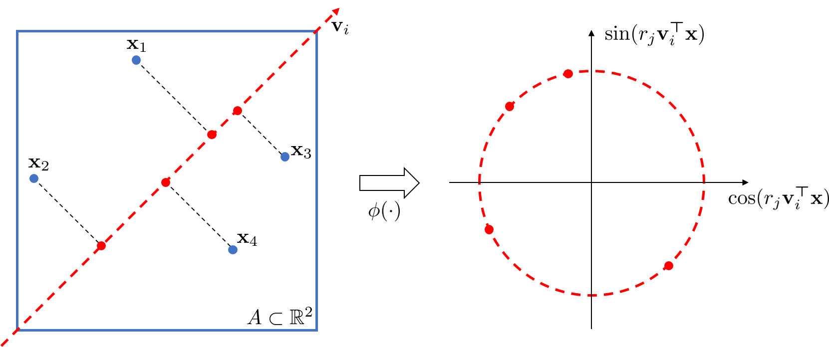
Figure 1: Our approximate mean kernel embedding can be seen as projecting the point pattern onto a line followed by the application of $\sin/\cos$ functions with the appropriate frequencies. The overall dimensionality of the resulting embedding is $D=2\times\mathrm{number\,of\,projections}\times\mathrm{number\,of\,frequencies}$. Figure adapted from [43].

The resulting pattern comparison test is surprisingly simple and a complete implementation is provided in the appendix. The computation of aKME is illustrated in Figure 1. First, the points in the pattern are projected onto a line, which is followed by the application of $\sin/\cos$ functions with a specific frequency; this step can be seen as wrapping the line onto a circle of some radius. The resulting $\sin/\cos$ values are separately averaged to give two numbers that provide a “fingerprint” of the point pattern behavior with respect to the direction of the line and the scale that corresponds to the frequency (i.e. circle circumference). The process is repeated with a multitude of lines and frequencies; assuming $m$ lines and $\ell$ frequencies per line, we obtain $m\ell$ such fingerprints; these are concatenated together to give an overall $D=2m\ell$ dimensional aKME. Finally, to compare patterns, we compare their aKMEs by applying $t$-tests on each coordinate of the embedding. We combine the resulting $D$ $p$-values into a single overall $p$-value using one of the recently introduced $p$-value combination techniques, such as harmonic mean [24, 53] or Cauchy combination test [39], leading to well-calibrated and powerful tests as confirmed by the simulations.

The connection to the original KME guides the choice of the parameters for this construction and provides approximation guarantees that are crucial to the consistency of the hypothesis testing. The main advantages of the proposed approach are that it can be applied to both single and replicated pattern comparisons, and that neither bootstrap nor permutation procedures are needed to obtain or calibrate the $p$-values. In addition, being based on $t$-tests, one can compute Bayes factors for each of the involved tests allowing to quantify evidence supporting the hypothesis of difference for each directionality/scale represented in aKME; one can also report the averaged Bayes factor as an overall summary of this evidence.

The ideas developed in this paper are in line with the recent surge of interest in applying reproducing kernel Hilbert space techniques to the comparison of probability distributions. For example, the Maximum Mean Discrepancy (MMD) is a measure of divergence between distributions [25] which has already found numerous applications in statistics and machine learning. This has led to the general approach of kernel mean embeddings, see for example the recent review [41] and citations therein. Some of these notions can be traced back and seen as closely related to N-distances [59] and energy distances [9, 48]. Our approximate embedding has its roots in the Random Fourier Features [43], its improvements [6, 56, 42], and its application to the MMD [58]; the scheme we propose in this paper is tailored to the two-dimensional setting, and has the ability to provide higher-order approximations. There has already been some interest in applying the reproducing kernel methodology to spatial point processes, the roots going back to the 1980s [10, 46] and more recently in [22, 35, 55]. We discuss some of the connections between reproducing kernel machinery and kernel density estimation based methods commonly used with spatial point patterns in Section 2.

The main contributions of this paper are the proposed approximate kernel mean embedding (Section 3) and the hypothesis testing framework for comparison of point patterns (Section 5). After investigating the empirical properties of the resulting tests on simulated data (Section 6.1), we present applications of the methodology to two real world datasets (Section 6.2).

2 Preliminaries

Kernel Mean Embedding

Mathematically rigorous development of the kernel mean embedding requires the machinery of the reproducing kernel Hilbert spaces, and the interested reader is referred to [41]. For our purposes, it will be sufficient to concentrate on the dual version of the definition where the kernel mean embedding is expressed in terms of the feature maps.

Given a data instance $\mathbf{x}\in\mathcal{X}$ (in our context $\mathbf{x}$ will be a point in some region of $\mathbb{R}^{2}$), a nonlinear transformation $\phi:\mathcal{X}\rightarrow\mathcal{F}$ can be used to lift this point into a feature space $\mathcal{F}$ that is usually high/infinite dimensional. When the entire dataset is lifted like this, the hope is that a good feature map would reveal structures in the dataset that were not apparent in the original space $\mathcal{X}$. For example, in the context of classification in machine learning, two classes that are hard to separate in the original space may turn out linearly separable in the feature space. This is the foundation of kernel based approaches in machine learning (see e.g. [31]), with the idea going back to [14].

Assuming that an inner product $\langle\cdot,\cdot\rangle$ is available on $\mathcal{F}$, with each feature map $\phi$ one can associate the kernel function $k:\mathcal{X}\times\mathcal{X}\rightarrow\mathbb{R}$ defined by $k(\mathbf{x},\mathbf{y})=\langle\phi(\mathbf{x}),\phi(\mathbf{y})\rangle$. It turns out that the converse is true as well: for each positive semi-definite (psd) kernel function $k(\cdot,\cdot)$ there exist a corresponding inner-product space $\mathcal{F}$ together with a feature map $\phi$ satisfying $k(\mathbf{x},\mathbf{y})=\langle\phi(\mathbf{x}),\phi(\mathbf{y})\rangle$.

For a given psd kernel $k(\cdot,\cdot)$, the kernel mean embedding (KME) of a probability distribution $p$ over $\mathcal{X}$ is defined as the expectation

$$\mu^{p}=\mathbb{E}_{\mathbf{x}\sim p}[\phi(\mathbf{x})]\in\mathcal{F}.$$

An important property of this embedding is that when $k(\cdot,\cdot)$ is a characteristic kernel, the embedding is injective [41]. In other words, for two distributions $p$ and $q$ over $\mathcal{X}$, the equality $\mu^{p}=\mu^{q}$ is satisfied if and only if $p=q$. This means that in the context of two-sample hypothesis testing, intuitively, the problem of testing whether $p=q$ can be reduced to testing $\mu^{p}=\mu^{q}$, albeit in the infinite-dimensional space $\mathcal{F}$.

Two-Sample Tests with KME

The absence of an explicit formula for $\phi$ and its infinite-dimensionality pose obstacles to devising an actual hypothesis testing procedure; fortunately, these can be overcome by using the kernel trick. Consider the distance (as induced by the inner-product in $\mathcal{F}$) between KMEs of $p$ and $q$, which is known as the Maximum Mean Discrepancy (MMD) [25]:

$$\mathrm{MMD}^{2}(p,q)=\|\mu^{p}-\mu^{q}\|^{2}.$$ (2.1)

The kernel trick, namely the application of the equality $k(\mathbf{x},\mathbf{y})=\langle\phi(\mathbf{x}),\phi(\mathbf{y})\rangle$, allows to express the MMD in terms of $k(\cdot,\cdot)$ without requiring an explicit formula for the feature map $\phi$, namely,

$$\mathrm{MMD}^{2}(p,q)=\mathbb{E}_{\mathbf{x},\mathbf{x}^{\prime}\sim p}[k(\mathbf{x},\mathbf{x}^{\prime})]-2\mathbb{E}_{\mathbf{x}\sim p,\boldsymbol{\mathbf{y}}\sim q}[k(\mathbf{x},\boldsymbol{\mathbf{y}})]+\mathbb{E}_{\mathbf{y},\mathbf{y}^{\prime}\sim q}[k(\mathbf{y},\mathbf{y}^{\prime})].$$ (2.2)

In practice this statistic is estimated from the samples by replacing the expectations with the sample means, with a nuance that the first and third terms can either include the diagonal terms or exclude them; the former gives a biased and the latter gives an unbiased estimator. Large enough values of $\mathrm{MMD}^{2}(p,q)$ provide evidence against the null hypothesis of $p=q$.

This has been an extremely fruitful approach to two-sample testing as witnessed by the vast amount of the follow-up work, see the references in [25, 41]. The distribution of MMD under the null hypothesis is not asymptotically normal nor has a practically useful explicit form except in big data settings where one can compute an incomplete estimator of MMD that is asymptotically normal; these cases are described in generality in [54]. As a result, in typical scenarios some kind of approximation or resampling procedure is required to perform the test, see [25] and pointers therein.

Connections to Kernel Density Estimation

The above described machinery has a close connection to kernel density estimation commonly used with spatial point patterns. For example, let us consider the two-sample test statistic proposed in [3], which was used by [20] in a three-dimensional setting and later adapted to the spatial point pattern comparison problem in [23]. This statistic is constructed by first obtaining kernel density estimates of the two distributions and then computing the squared $L^{2}$-distance between the density estimates. Its connection to MMD is described in [25, Section 3.3.1] and can be exemplified as follows: if, say, the kernel density estimate is based on the Gaussian kernel of bandwidth $\sigma$, then this statistic is equivalent to the MMD computed with the same kernel but of bandwidth $\sqrt{2}\sigma$. Overall, MMD statistic is strictly more general than the statistic of [3] because it allows using a larger variety of kernels; another benefit is the stronger consistency guarantees that stem from the kernel mean embedding interpretation. Similarly to the MMD, the statistic of [3] is not asymptotically normal under the null; nevertheless, a normal approximation was suggested in [20]. However, this approximation leads to severe calibration problems: [23] reported conservativeness of the resulting test, which led them to rely on bootstrap for calibration.

Of course, instead of the $L^{2}$-distance, other distances can be computed between the kernel density estimates to obtain statistics that capture complementary aspects of the differences between distributions. Similarly, one can realize that the MMD captures only one aspect of the discrepancy between the kernel mean embeddings. For example, the kernel Fisher discriminant analysis (KFDA) test statistic [21] is another statistic that can be computed via the kernel trick and used to test the equality $\mu^{p}=\mu^{q}$. Similarly to the relationship between MMD and the squared $L^{2}$-distance, the KFDA is connected to the $\chi^{2}$-distance between kernel density estimates. An insightful review of this type of connections can be found in [30].

3 Approximate Kernel Mean Embedding

Instead of relying on the kernel trick, in this section we take an orthogonal path to avoiding the infinite-dimensionality of the kernel mean embedding. Namely, specializing to the case $\mathcal{X}=\mathbb{R}^{2}$, we construct a finite-dimensional approximate feature map $\phi:\mathbb{R}^{2}\rightarrow\mathbb{R}^{D}$ such that $k(\mathbf{x},\mathbf{y})\approx\phi(\mathbf{x})^{\boldsymbol{\top}}\phi(\mathbf{y})$. As a result, testing $p=q$ can be reduced to testing $\mu^{p}=\mu^{q}$ in the $D$-dimensional Euclidean space.

Since it allows obtaining closed form formulas, for the rest of the paper we will concentrate on the Gaussian kernel $k(\mathbf{x},\mathbf{y})=e^{-\|\mathbf{x}-\mathbf{y}\|^{2}/2\sigma^{2}}$ for $\mathbf{x},\mathbf{y}\in\mathbb{R}^{2}$. To avoid clutter in the derivations the kernel bandwidth $\sigma$ is assumed to be $1$; the case of general $\sigma$ is mentioned below. Our goal is to construct an approximate feature map for the Gaussian kernel tailored to the two-dimensional case. As a starting point, following the notation from [42] let us write the Gaussian kernel as

$$k(\mathbf{x},\mathbf{y})=\frac{1}{2\pi}\int_{-\infty}^{\infty}\int_{-\infty}^{\infty}e^{-\frac{\mathbf{w}^{\boldsymbol{\top}}\mathbf{w}}{2}}\cos(\mathbf{w}^{\boldsymbol{\top}}(\mathbf{x}-\mathbf{y}))d\mathbf{w}=\frac{1}{2\pi}\int_{-\infty}^{\infty}\int_{-\infty}^{\infty}e^{-\frac{\mathbf{w}^{\boldsymbol{\top}}\mathbf{w}}{2}}\eta(\mathbf{w}^{\boldsymbol{\top}}\mathbf{x})^{\boldsymbol{\top}}\eta(\mathbf{w}^{\boldsymbol{\top}}\mathbf{y})d\mathbf{w},$$

where $\eta(\cdot)=\left[\begin{array}[]{cc}\cos(\cdot)&\quad\sin(\cdot)\end{array}\right]{}^{\boldsymbol{\top}}$. To compress the notation, let $f(\mathbf{w})=\eta(\mathbf{w}^{\boldsymbol{\top}}\mathbf{x})^{\boldsymbol{\top}}\eta(\mathbf{w}^{\boldsymbol{\top}}\mathbf{y})$ where the dependence on $\mathbf{x}$ and $\mathbf{y}$ is suppressed from the notation. We change to the radial coordinates, and notice that $f$ is an even function to obtain:

$$k(\mathbf{x},\mathbf{y})=\frac{1}{2\pi}\int_{0}^{2\pi}\int_{0}^{\infty}re^{-\frac{r^{2}}{2}}f(r\mathbf{z_{\theta}})drd\mathbf{\theta}=\frac{1}{\pi}\int_{0}^{\pi}\int_{0}^{\infty}re^{-\frac{r^{2}}{2}}f(r\mathbf{z_{\theta}})drd\mathbf{\theta},$$

where $\mathbf{z}_{\theta}$ is a unit vector in $\mathbb{R}^{2}$ making an angle of $\theta$ with the $x$-axis. We approximate the integration with respect to $\theta$ by the simple mean over a set of equidistant values $\theta_{i}=(i-1)\pi/m$, $i=1,2,....,m$. Let $\mathbf{v}_{i}=\mathbf{z}_{\theta_{i}}$ to get

$$k(\mathbf{x},\mathbf{y})\approx\sum_{i=1}^{m}\int_{0}^{\infty}re^{-\frac{r^{2}}{2}}f(r\mathbf{v}_{i})dr.$$

Now we use a radial version of Gauss-Hermite quadrature to compute the integral over $r$ [33]. For a given integer $\ell\geq 1$, denoting the quadrature roots by $\{r_{j}\}_{j=1}^{\ell}$ and the corresponding weights by $\{\omega_{j}\}_{j=1}^{\ell}$, we obtain

$$k(\mathbf{x},\mathbf{y})\approx\sum_{i=1}^{m}\sum_{j=1}^{\ell}\omega_{j}f(r_{j}\mathbf{v}_{i})=\sum_{i=1}^{m}\sum_{j=1}^{\ell}\omega_{j}\eta(r_{j}\mathbf{v}_{i}^{\boldsymbol{\top}}\mathbf{x})^{\boldsymbol{\top}}\eta(r_{j}\mathbf{v}_{i}^{\boldsymbol{\top}}\mathbf{y}).$$

The crucial point is that the terms containing $\mathbf{x}$ and $\mathbf{y}$ are untangled, which allows us to write $k(\mathbf{x},\mathbf{y})$ approximately as a dot product in the embedding space: $k(\mathbf{x},\mathbf{y})\approx\phi_{m,\ell}(\mathbf{x})^{\top}\phi_{m,\ell}(\mathbf{y})$, where $\phi_{m,\ell}:\mathbb{R}^{2}\rightarrow\mathbb{R}^{D}$, $D=2m\ell$ is explicitly given by

$$\phi_{m,\ell}(\mathbf{x})=[...,\sqrt{\omega_{j}}\sin(r_{j}\mathbf{v}_{i}^{\boldsymbol{\top}}\mathbf{x}),\sqrt{\omega_{j}}\cos(r_{j}\mathbf{v}_{i}^{\boldsymbol{\top}}\mathbf{x}),...]^{\top},$$

where in total there are $m\ell$ sine/cosine pairs corresponding to all combinations of $i$ and $j$. We note that the case of the Gaussian kernel with the width $\sigma$ can be accommodated by replacing $\mathbf{x}$ with $\mathbf{x}/\sigma$. To avoid committing to a single $\sigma$, in practice, one can construct multiple feature maps corresponding to different values of the kernel width, and concatenate the resulting vectors together to obtain a higher dimensional embedding (e.g. using three different width values results in a $3D$-dimensional embedding).

The connection to Random Fourier Features [43] should be obvious from the form of our embedding. Note that the construction in [43] and its improvements [6, 56, 42] are geared towards high-dimensional data and, thus, depend on stochasticity to avoid the curse of dimensionality. In contrast, our construction is tailored to the two-dimensional setting and is based on a deterministic quadrature rule that quickly provides a high-order approximation. For example, considering a region $A\subset\mathbb{R}^{2}$ the approximation error of the kernel function can be bounded as

$$|k(\mathbf{x},\mathbf{y})-\phi_{m,\ell}(\mathbf{x})^{\top}\phi_{m,\ell}(\mathbf{y})|\leq C_{1}\frac{\|x-y\|}{m}+C_{2}\gamma_{\ell}\frac{\|x-y\|^{2\ell}}{(2\ell)!}\leq\epsilon(m,\ell,\mathrm{diam}(A)),$$

for all $\mathbf{x},\mathbf{y}\in A$. The first term comes from the classical Riemann sum approximation error and the second term is the standard form for general Gaussian quadrature (Theorem 3.6.24 in [47]); the powers of $\|x-y\|$ arise from differentiation of the integrand. When using kernel width of $\sigma$, the error depends on $\mathrm{diam}(A)/\sigma$. Our bound reflects the quality of the quadrature rules involved in the approximation scheme, and so is conceptually different from the probabilistic bound in [43]. There is quantitative difference as well: their dimension $D$ to achieve error $\epsilon$ scales roughly as $\epsilon^{-2}\log\epsilon$, whereas ours as $\epsilon^{-1}\log\epsilon$. As a result, the proposed embedding is able to capture more information about the distribution for the same number of dimensions, resulting in more powerful tests. Nevertheless, the hypothesis tests proposed in Section 5 do generalize to Random Fourier Feature based embeddings and, consequently, can be applied in high-dimensional settings.

Having introduced the approximate feature map, we can define the approximate kernel mean embedding (aKME) of a probability distribution $p(\cdot)$ over the region $A\subset\mathbb{R}^{2}$ as $\mathrm{aKME}_{m,\ell}(p)=\mu_{m,\ell}^{p}=\mathbb{E}_{\mathbf{x}\sim p}[\phi_{m,\ell}(\mathbf{x})]\in\mathbb{R}^{D}$. For two distributions $p$ and $q$ over $A$,

$$\mathrm{MMD}^{2}(p,q)\approx\|\mathrm{aKME}_{m,\ell}(p)-\mathrm{aKME}_{m,\ell}(q)\|^{2},$$ (3.1)

where in contrast to Eq. (2.1) the embeddings on the right-hand side are computed via aKME. The approximation error can be estimated by replacing each term of Eq. (2.2) with their approximations ($\mathbb{E}_{\mathbf{x},\mathbf{x}^{\prime}\sim p}[k(\mathbf{x},\mathbf{x^{\prime}})]\approx\mathbb{E}_{\mathbf{x},\mathbf{x}^{\prime}\sim p}[\phi_{m,\ell}(\mathbf{x})^{\top}\phi_{m,\ell}(\mathbf{x}^{\prime})]$ and so on), which incurs an overall error upper-bounded by $4\epsilon(m,\ell,\mathrm{diam}(A))$. The expectations decouple ($\mathbb{E}[\phi_{m,\ell}(\mathbf{x})^{\top}\phi_{m,\ell}(\mathbf{x}^{\prime})]=\mathbb{E}_{x\sim p}[\phi_{m,\ell}(\mathbf{x})^{\top}]\mathbb{E}_{x^{\prime}\sim p}[\phi_{m,\ell}(\mathbf{x}^{\prime})]$ and so on) yielding Eq. (3.1) after some algebra; see [58] for a similar argument in the Random Fourier Features context.

For a large class of probability distributions, $p\neq q$ implies $\mathrm{MMD}^{2}(p,q)>0$ [25]. Thus, by taking $m$ and $\ell$ large enough so that the approximation error $4\epsilon(m,\ell,\mathrm{diam}(A))$ of Eq. (3.1) is small enough we will obtain $\|\mathrm{aKME}_{m,\ell}(p)-\mathrm{aKME}_{m,\ell}(q)\|^{2}>0$ which implies $\mathrm{aKME}_{m,\ell}(p)\neq\mathrm{aKME}_{m,\ell}(q)$. In other words, if two distributions are different, this difference will be discerned by the aKME of high enough dimensionality. This property of our construction will be crucial when proving the consistency of the proposed hypothesis tests.

Remark

To simplify notation, in the subsequent sections we will drop the subscripts $m$ and $\ell$ from all of the approximate constructs.

4 Spatial Point Pattern aKME

The goal of this section is to introduce the aKME for a point process and show that it can be estimated in an unbiased manner from the realizations of the point process. As a preliminary, we have to compare the notions of the first-order intensity and the density of event locations for spatial point processes. While for an inhomogeneous Poisson process these two are equivalent up to a normalization, in general there are differences that should be taken into consideration when conducting replicated pattern comparisons.

Intensity versus Location Density

Let $P$ be a point process on the region $A\subset\mathbb{R}^{2}$. The first-order intensity function $\lambda^{P}(\cdot$) of this process is defined as

$$\lambda^{P}(\mathbf{x})=\lim_{|dx|\to 0}\frac{\mathbb{E}[N(d\mathbf{x})]}{|d\mathbf{x}|},$$

where $d\mathbf{x}$ is a neighborhood around $\mathbf{x}$, and $N(\cdot)$ is the count of events and $|\cdot|$ is the area. The definition of the density of event locations, or simply, location density function $p(\cdot)$, is as follows:

$$p(\mathbf{x})=\lim_{|d\mathbf{x}|\to 0}\frac{\mathbb{E}[N(d\mathbf{x})/N(A)]}{|d\mathbf{x}|},$$

note the normalization by the overall number of points. It is easy to see that $p(x)$ integrates to 1 over $A$, and as such is a probability density function on $A$.

To clarify the connection between $\lambda^{P}$ and $p$ we can rewrite the definition by conditioning on the number of events in a point pattern:

$$p(\mathbf{x})=\lim_{|d\mathbf{x}|\to 0}\frac{\mathbb{E}[N(d\mathbf{x})/N(A)]}{|d\mathbf{x}|}=\mathbb{E}_{n}\left[\frac{1}{n}\lim_{|d\mathbf{x}|\to 0}\frac{\mathbb{E}_{N(A)=n}[N(d\mathbf{x})]}{|d\mathbf{x}|}\right]=\mathbb{E}_{n}\left[\frac{1}{n}\lambda^{P}(\mathbf{x}|N(A)=n)\right],$$ (4.1)

where $\lambda^{P}(\mathbf{x}|N(A)=n)$ is the first-order intensity conditioned on the total number of points in the pattern being equal to $n$.

For an inhomogeneous Poisson process, the intensity and the location density are equivalent up to normalization. Indeed, consider a Poisson process $P$ on $A$ with intensity $\lambda^{P}(\cdot$) and denote $\beta=\int_{A}\lambda^{P}(\mathbf{x})d\mathbf{x}$. Conditioning a Poisson process to have $n$ points gives the binomial process with intensity $n\lambda^{P}(\cdot)/\beta$. Plugging this into Eq. (4.1), we get $p(\cdot)=\lambda^{P}(\cdot)/\beta$.

Turning to the non-Poisson case, we see that if the condition

$$\lambda^{P}(\mathbf{x}|N(A)=n)=n\frac{\lambda^{P}(\mathbf{x})}{\int_{A}\lambda^{P}(\mathbf{x})d\mathbf{x}}\quad\forall n\>\mathrm{such\>that}\>\mathbf{\mathrm{Prob}}(N(A)=n)>0$$ (4.2)

holds, the above argument can be repeated verbatim to give the equivalence between intensity and location density: $p(\cdot)=\lambda^{P}(\cdot)/\int_{A}\lambda^{P}(\mathbf{x})d\mathbf{x}$. We will provide a detailed discussion of this requirement at the end of this section.

Spatial Point Pattern aKME

The aKME of the point process $P$ is defined via the embedding of its location density function $p(\cdot)$, namely, $\mu^{P}=\mu^{p}=\mathbb{E}_{\mathbf{x}\sim p}[\phi(\mathbf{x})]\in\mathbb{R}^{D}.$ In practice, we only have access to a point process via its realizations, and so, we must be able to estimate the aKME in an unbiased manner from a point pattern; this is the focus of the following discussion.

Consider a realization $\boldsymbol{X}=\{\mathbf{x}_{1},\mathbf{x}_{2},...,\mathbf{x}_{n}\}$ of the point process $P$. The estimator that we will be interested in is the one that replaces the expectation appearing in the aKME formula by the sample mean:

$$\hat{\mu}^{\boldsymbol{X}}=\frac{1}{n}\sum_{j=1}^{n}\phi(\mathbf{x}_{j})\in\mathbb{R}^{D}.$$ (4.3)

We require this estimate to be unbiased, $\mathbb{E}_{\mathbf{X}\sim P}[\hat{\mu}^{\boldsymbol{X}}]=\mu^{p}$, where the expectation is taken over the realizations of the process $P$. Unbiasedness is essential as it ensures that the estimate $\hat{\mu}^{\boldsymbol{X}}$ captures information about the location density function rather than some other properties of the point process.

Next, we prove that unbiasedness holds for any point process that satisfies the condition of Eq. (4.2). We can write,

$$\mathbb{E}_{\boldsymbol{X}\sim P}[\hat{\mu}^{\boldsymbol{X}}]=\mathbb{E}_{n}\left[\frac{1}{n}\mathbb{E}_{\boldsymbol{X}\sim P,|\mathbf{X}|=n}\left[\sum_{j=1}^{n}\phi(\mathbf{x}_{j})\right]\right].$$

Using Campbell’s formula and Eq. (4.2), we get

$$\frac{1}{n}\mathbb{E}_{\boldsymbol{X}\sim P,|\mathbf{X}|=n}\left[\sum_{j=1}^{n}\phi(\mathbf{x}_{j})\right]=\frac{1}{n}\int_{A}\phi(\mathbf{x})\lambda^{P}(\mathbf{x}|N(A)=n)d\mathbf{x}=\int_{A}\phi(\mathbf{x})p(\mathbf{x})d\mathbf{x}.$$

Substituting this back,

$$\mathbb{E}_{\boldsymbol{X}\sim P}[\hat{\mu}^{\boldsymbol{X}}]=\mathbb{E}_{n}\left[\int_{A}\phi(\mathbf{x})p(\mathbf{x})d\mathbf{x}\right]=\int_{A}\phi(\mathbf{x})p(\mathbf{x})d\boldsymbol{\mathbf{x}}=\mathbb{E}_{\mathbf{x}\sim p}[\phi(\mathbf{x})]=\mu^{p},$$

which proves that the estimator is unbiased.

Discussion

The equivalence between the first-order intensity and the location density functions implied by Eq. (4.2) is important for our hypothesis tests, as we replace the comparison of intensities by the comparison densities; we also saw that Eq. (4.2) is at the core of estimating aKME in an unbiased manner. Thus, the validity of our hypothesis testing framework in Section 5 hinges on this condition, and so it requires further discussion. Our single pattern comparison test assumes that patterns are sampled from (in-)homogeneous Poisson processes. We already saw that inhomogeneous Poisson processes satisfy this property, which validates our single comparison test. On the other hand, our replicated pattern comparison test can be used for non-Poisson processes, and so one has to ascertain that the condition of Eq. (4.2) holds.

Here we focus on a practical discussion and leave theoretical analysis of this requirement to the future work. We loosely express the requirement of Eq. (4.2) as follows: conditioning on the number of points in the pattern does not have an effect on the functional form of the first-order intensity (i.e. it induces a change by a constant factor). The simplicity of this requirement makes it possible to use domain knowledge to assess how likely it is to hold in practice. For example, non-Poisson point processes are common in plant biology applications; the functional form of the first-order intensity is determined by the environmental factors such as light conditions, level of water underground, and quality of soil. Thus, conditioning on the total number of plants in the region of interest should not affect the first-order intensity except for an overall constant factor, which makes it plausible to assume that the condition highlighted above holds.

A similar argument can be made for patterns of a certain type of crime in a town on a fixed day of the week. However, if we were to consider the patterns without regard for the day of the week then violations of Eq. (4.2) are possible. To this end, consider a scenario where: 1) the number of crimes on weekends is typically much lower than on weekdays, and 2) crimes on weekdays typically happen in the residential areas and on weekends in the business areas. Thus, conditioning on the number of events in a pattern effectively splits the patterns by weekday/weekend, and the corresponding event intensities concentrate on different parts of the town, resulting in the failure of the requirement above.

In data rich regimes one can use the following strategy to asses the requirement of Eq. (4.2). One can group the collection of patterns by the number of events, so that patterns in the same group do not differ drastically in the number of events. Next, our replicated pattern comparison test can be applied to each pair of groups to determine if there are inter-group differences in the location densities. If no significant differences are found, then one can assume that the overall set of patterns satisfies the condition of Eq. (4.2). The approximate validity of this approach stems from the following observation. An obvious case where the requirement trivially holds is when every realization of the process has the same number of events. Based on this, we conjecture that in practical situations having small differences in the counts of events in the patterns should not lead to big violations of the requirement allowing us to use the test.

5 Comparing Spatial Point Patterns with aKME

Consider two point processes $P$ and $Q$ in $A\subset\mathbb{R}^{2}$ with the first-order intensity functions given by $\lambda^{P}(\cdot$) and $\lambda^{Q}(\cdot)$. We would like to test the null hypothesis of whether there exists a constant $c$ such that $\lambda^{P}(\cdot)=c\lambda^{Q}(\cdot)$. Equality up to a constant factor means that the intensities of the two processes have the same functional form. This is different from testing $\lambda^{P}(\cdot)=\lambda^{Q}(\cdot)$ because our null hypothesis can hold true even if the realizations from $P$ and $Q$ have vastly differing numbers of events. We start with the Poisson case that allows testing based on a single realization per process and proceed to replicated pattern comparison that is applicable more generally.

Single Pattern Comparison

Assume that we observe two patterns $\boldsymbol{X}=\{\mathbf{x}_{1},\mathbf{x}_{2},...,\mathbf{x}_{n_{1}}\}$ and $\boldsymbol{Y}=\{\mathbf{y}_{1},\mathbf{y}_{2},...,\boldsymbol{\mathbf{y}}_{n_{2}}\}$ from two inhomogeneous Poisson processes $P$ and $Q$ on the region $A\subset\mathbb{R}^{2}$ with the true intensity functions given by $\lambda^{P}(\cdot$) and $\lambda^{Q}(\cdot)$. We would like to test the null hypothesis of whether there exists a constant $c$ such that $\lambda^{P}(\cdot)=c\lambda^{Q}(\cdot)$. Using the equivalence between intensities and location densities of Poisson processes proved in Section 4, the location density functions $p(\cdot)$ and $q(\cdot)$ are obtained from the intensities $\lambda^{P}(\cdot$) and $\lambda^{Q}(\cdot)$ via normalization (e.g. $p(\cdot)=\lambda^{P}(\cdot)/\int_{A}\lambda^{P}(\mathbf{x})d\mathbf{x}$). Clearly, the null hypothesis above can be written as $p=q$.

Applying the aKME machinery, we reduce the test to checking whether $\mu^{p}=\mu^{q}$ in the $D$-dimensional Euclidean space. While the classic Hotelling’s $T^{2}$ test seems like a natural choice, yet given the high-dimensionality of our embedding this becomes very data hungry; in practice the computation of the precision matrix turns out to be unstable. We also tried using a test geared to the high-dimensional setting [13], but it failed to control the size of the test due to the nonlinear relationships between the coordinates of the approximate feature map which breaks the multivariate normality assumption.

To avoid these issues we perform the test by applying $t$-tests independently to each coordinate and combining the resulting $p$-values as explained below. More precisely, for each coordinate $i=1,2,...,D$, by Poisson assumption we can consider $\{\phi_{i}(\mathbf{x}_{j}),\mathbf{x}_{j}\in\boldsymbol{X}\}$ and $\{\phi_{i}(\mathbf{y}_{j}),\mathbf{y}_{j}\in\boldsymbol{Y}\}$ to be two independent samples of sizes $n_{1}$ and $n_{2}$ respectively; here $\phi_{i}$ is the $i$-th coordinate of the approximate feature map. Our goal is to compare the sample means $\hat{\mu}_{i}^{\boldsymbol{X}}$ and $\hat{\mu}_{i}^{\boldsymbol{Y}}$. Note that since the approximate feature maps are expressed in terms of sines and cosines, their range is bounded, and so the classical Central Limit Theorem can be applied to deduce the approximate normality of the sample means $\hat{\mu}_{i}^{\boldsymbol{X}}$ and $\hat{\mu}_{i}^{\boldsymbol{Y}}$ when the sample sizes are big enough. As a result, we can apply the Behrens-Fisher-Welch $t$-test (without assuming equality of variances) to obtain the corresponding $p$-value $p_{i}$.

All together we end up with a set of $p$-values $p_{1},p_{2},...,p_{D}$ one per coordinate of the aKME. In principle, one can resort to multiple testing procedures to reject or retain the global null. However, it is useful to compute an overall $p$-value for the the global null hypothesis $\mu^{p}=\mu^{q}$ so that it can be used in downstream multiple testing procedures. To obtain such an overall $p$-value we use one of the $p$-value combination approaches, see Eqs. (5.1) and (5.2) at the end of this section. Using the approximation properties of aKME we prove in Appendix A that the proposed test is consistent.

Replicated Pattern Comparison

In the replicated pattern setting we can abandon the Poisson assumption; the only assumption on the involved point processes is that condition of Eq. (4.2) holds. Here, for two such general processes $P$ and $Q$ on the region $A\subset\mathbb{R}^{2}$ with true intensity functions given by $\lambda^{P}(\cdot$) and $\lambda^{Q}(\cdot)$, we observe a set of patterns $P^{*}=\{\boldsymbol{X}_{1},\boldsymbol{X}_{2},...,\boldsymbol{X}_{m_{1}}\}$ and $Q^{*}=\{\boldsymbol{Y}_{1},\boldsymbol{Y}_{2},...,\boldsymbol{Y}_{m_{2}}\}$ independently drawn from $P$ and $Q$ respectively. Our goal is to test whether $\lambda^{P}(\cdot)=c\lambda^{Q}(\cdot)$. As proved in Section 4, the equivalence between intensities and location densities holds, and so the problem can be reduced to testing $p=q$ exactly as before.

In this setting, we can consider the collection of each coordinate $i$ of the aKME embeddings $\{\hat{\mu}_{i}^{\boldsymbol{X}_{k}},\boldsymbol{X}_{k}\in P^{*}\}$ and $\{\hat{\mu}_{i}^{\boldsymbol{Y}_{k}},\boldsymbol{Y}_{k}\in Q^{*}\}$ as independent samples of sizes $m_{1}$ and $m_{2}$. Being the means of sines and cosines, the range of each coordinate is bounded, but in contrast to the previous case the means coming from different replications are not identically distributed due to the varying number of events in each replication. Uniform boundedness and independence allow us to apply the Lyapunov/Lindeberg version of the Central Limit Theorem [12, Chapter 27] to deduce the approximate normality of the sample means when the sample sizes (i.e. the number of replications of patterns) are big enough. This allows us to test for the equality of the $i$-th coordinates $\mu_{i}^{p}=\mu_{i}^{q}$ using the $t$-test. Here, the validity of the $t$-test stems from independence of replications and holds for general processes; this should be contrasted to the single pattern comparison test above which derives its validity from the independence of samples within a single pattern in the Poisson process. The set of $D$ $p$-values obtained from the $t$-tests are combined using one of the $p$-value combination approaches discussed below to obtain an overall $p$-value.

We finish with an important remark about the nature of this test. The point processes $P$ and $Q$ do not have to be of the same type for the null hypothesis to hold. The test is concerned only with the functional form of the intensity, and not the type of the process. For example, if $P$ is an inhibition process and $Q$ is a cluster process, then the null hypothesis still holds as long as the first-order intensity functions of these processes are the same up to a constant factor; having it otherwise would have implied that the test conflates higher order properties with the first order properties.

Combining P-Values

To obtain an overall $p$-value for the tests described above, we need to combine the per-coordinate $p$-values $p_{1},p_{2},...,p_{D}$ in a manner that is robust to the dependencies between them. We found experimentally that classical $p$-value combination approaches such as Fisher’s and Stouffer’s methods (see, e.g. [40, 32]) fail to give well-calibrated $p$-values likely due to their strong reliance on the independence assumption. In contrast, the recently introduced combination techniques, harmonic mean $p$-value [24, 53] and Cauchy combination test [39] resulted in well-calibrated tests with better power than simple alternatives such as the Bonferroni adjustment for multiple testing. We quickly review these approaches and provide some insight into their behavior and the relationship between them.

The harmonic mean $p$-value combination approach defines an overall $p$-value by

$$p^{H}=H\left(\frac{D}{\frac{1}{p_{1}}+\frac{1}{p_{2}}+\cdots+\frac{1}{p_{D}}}\right),$$ (5.1)

where $H(\cdot)$ is a function whose precise form is described in [53]. Since $H(x)\approx x$ for small values of $x$, $p^{H}$ is approximately the harmonic mean of $p_{1},p_{2},...,p_{D}$. On the other hand, the Cauchy combination test defines an overall $p$-value by the formula

$$p^{C}=\frac{1}{\pi}\cot^{-1}\left(\frac{\cot\pi p_{1}+\cot\pi p_{2}+\cdots+\cot\pi p_{D}}{D}\right),$$ (5.2)

where $\cot$ is the cotangent function, $\cot x=\tan(\pi/2-x)$. In contrast to classical combination techniques, both of these approaches are shown to be robust when there are dependencies between the individual $p$-values $p_{1},p_{2},...,p_{D}$ [53, 39].

Curiously, these two methods behave very similarly for small $p$-values. Indeed, we can rewrite Eq. (5.2) as $D\cot\pi p^{C}=(\cot\pi p_{1}+\cot\pi p_{2}+\cdots+\cot\pi p_{D})$. For small $x$, the approximation $\cot x\approx 1/x$ can be used, and canceling out $\pi$s on both sides we get $D/p^{C}\approx 1/p_{1}+1/p_{2}+\cdots+1/p_{D}$. It follows that $p^{C}$ is approximately the harmonic mean of $p_{1},p_{2},...,p_{D}$, and, therefore, $p^{C}\approx p^{H}$.

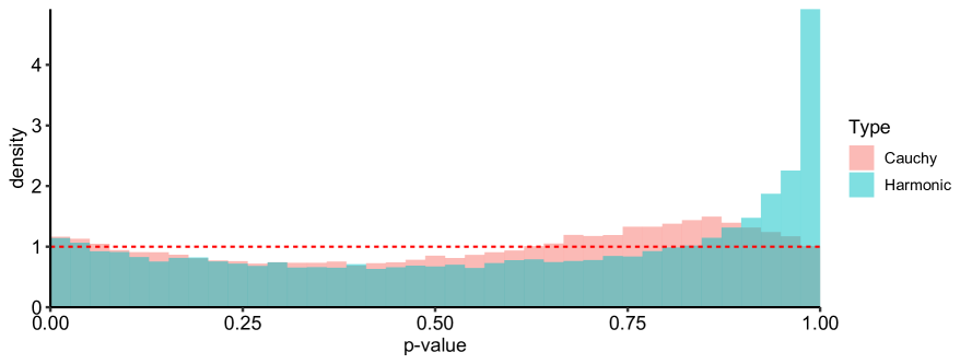
Figure 2: Distribution of combined $p$-values under the null for the Poisson process experiment in Section 6.1.

To gain some more intuition about the behavior of these techniques we can look at the distribution of the combined $p$-values under the null. Figure 2 depicts the histogram of combined $p$-values corresponding to the Poisson process experiment in Section 6.1 when the null holds. It can be seen that the methods behave very similarly for small values of $p$ as expected from the approximation argument above. Both of the combination approaches result in unit density for small values of $p$, which makes them equally suitable for hypothesis testing (c.f. “Size” portion of Table 1). Interestingly, the harmonic mean approach leads to overcrowding of $p$-values near $1$, whereas the Cauchy combination $p$-values stay more or less uniformly distributed. The large $p$-value behavior can in general be ignored in the context of hypothesis testing. However, it can be a consideration when using adaptive false discovery control techniques based on the mirroring technique [8, 5] that relies on symmetric distribution of $p$-values near $0$ and $1$. Otherwise, the harmonic mean approach has a number of advantages, including a Bayesian model-averaging interpretation and its being an inherently multilevel test [53].

Due to their similar behavior in the relevant regime, we use the harmonic mean $p$-value approach in all of the experiments presented in the paper. The sample source code provided in Appendix B demonstrates the calculation for both of the $p$-value combination techniques.

Adjusting $p$-values

While the $p$-value combination methods above give excellent results in practice and are fast to compute, their approximate nature and the resulting non-uniformity of $p$-values over the entire range can potentially be a problem in some applications. Here we present two adjustment approaches to obtaining guaranteed size control. Let us emphasize that we do not use any adjustments in the experiments reported in the main text.

The first approach is based on the worst-case performance of $p$-value combination techniques [50] and will lead to rather conservative tests. For example, using the Bonferroni adjustment is equivalent to using the combined $p$-value $p^{B}=D\min\{p_{1},p_{2},...,p_{D}\}$. For the pure harmonic mean combination (i.e. without the application of function $H$ in Eq. (5.1)) it holds that $a^{H}(D)p^{H}$ provides guaranteed size control for some factor $a^{H}(D)$ that depends on the number of the $p$-values being combined [50]; there is no closed-form formula for this factor, but it satisfies $a^{H}(D)\leq e\ln D$ and $\lim_{D\to\infty}a^{H}(D)/\ln D=1$.

Another method is to adjust the $p$-values using resampling. Focusing on the harmonic approach, our test statistic would be the harmonic combination $p$-value. We generate $B$ samples of the harmonic $p$-value $\{p_{b}^{H}\}_{b=1}^{B}$ from the null distribution. Given the observed value of $p^{H}$ for the comparison at hand, we compute the adjusted harmonic $p$-value via the formula $p^{AH}=(|\{b:p_{b}^{H}\leq p^{H}\}|+1)/(B+1)$. The generation of the null distribution is guided by the test and a choice between randomized permutation or bootstrap. For single pattern comparison, we can either randomly shuffle points across the two point patterns or sample points with replacement from the aggregation of the two patterns (smoothed bootstrap can be used by estimating the location density of the aggregate pattern); for replicated pattern comparison we can similarly either shuffle the patterns across the groups or sample patterns with replacement from the overall pattern pool. Note that the resampling approach can be used in cases where the Poisson assumption (required for single pattern comparison) fails as long as one can generate a valid null distribution by techniques such as tiled resampling [29].

Bayes Factors

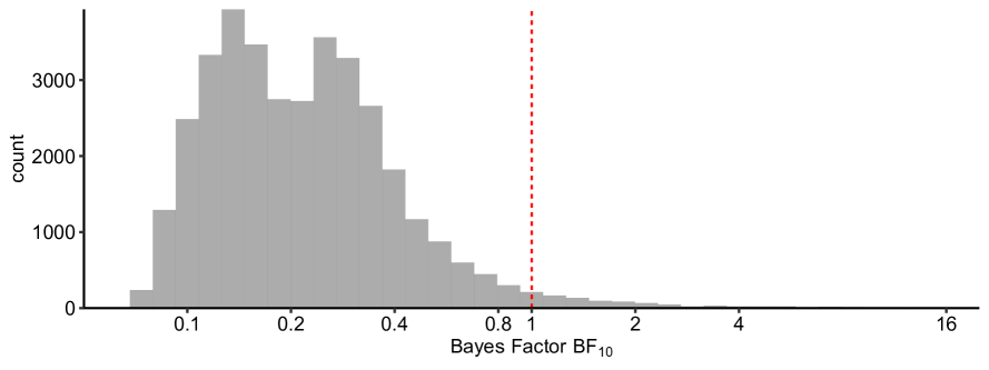
Figure 3: Distribution of mean Bayes factors under the null for the Poisson process experiment in Section 6.1. The $x$-axis has logarithmic scale. As expected, these values are overwhelmingly below 1, shown by a red line.

Each dimension of the aKME captures the behavior of the point pattern in a specific direction at a specific scale. Thus, Bayesian approaches can potentially be used for hypothesis testing with priors that capture the beliefs for differences along each dimension of the aKME. To illustrate this idea, we follow a straightforward approach and rely on the existing default priors for $t$-test (e.g. [45]) to compute Bayes factors [34, 36] for each dimension of the aKME. Next, we combine these Bayes factors following the work of [51] via arithmetic mean to obtain what Vovk and Wang call an $e$-value; we will refer to this quantity as the mean Bayes factor and will denote it by $\overline{\mathrm{BF}}_{10}$. In essence, $\overline{\mathrm{BF}}_{10}$ captures the overall evidence against the null hypothesis and under the null it is expected to be smaller than 1. We confirm this by computing the mean Bayes factors for the null cases of Poisson process experiment in Section 6.1. Figure 3 shows the histogram of the resulting $\overline{\mathrm{BF}}_{10}$ values and demonstrates that under the null they overwhelmingly take values smaller than 1. We will report mean Bayes factors for the real world experiments in Section 6.2.

6 Experiments

Our goal in this section is to investigate the size and the power of the proposed tests. We also demonstrate two applications to real world data. The aKME embedding is constructed using four radial projections and four roots for the polar Gauss-Hermite formula (i.e. $m=4$, $\ell=4$ in the notation of Section 3) resulting in $D=32$. To avoid the selection of the kernel width parameter, we concatenate together aKMEs corresponding to $\sigma=1/16,1/8,$ and $1/4$ when the point pattern domain is the unit square; the dimensionality of the concatenated aKME is $3\times 32=96$. To motivate these choices of $\sigma$, notice that the spatial scales represented in aKME correspond to the periods of the involved trigonometric functions and have the form $2\pi\sigma/r_{j}$. Consulting the values for $r_{j}$ from the source code in Appendix B, we see that the corresponding spatial scales vary from approximately $0.1$ to $4$, which we expect would reveal differences between patterns considered here. All of these values except for two are under $\sqrt{2}$ (diagonal of the square); while those two largest values may seem redundant, they are required for revealing the gross differences between patterns when they exist.

6.1 Simulations

Single Pattern Comparison

We generate two types of inhomogeneous Poisson processes (Linear and Sine) on the unit square $[0,1]\times[0,1]$ with the intensity functions given by $\exp(-\gamma x)$ and $\exp(-\gamma\sin(2\pi x))$, where $x$ is the abscissa; the form of these is borrowed from [27]. Here, $\gamma$ takes the values of $\gamma=1,2,3$; the intensity functions are normalized so that the expected number of points per realization is $100$, $400$ or $800$. For each pair of parameter settings being compared the model is simulated 2000 times.

							This Paper						Zhang and Zhuang						Fuentes-Santos et al.
Model	$\beta_{1}$	$\beta_{2}$	$\lambda$				$\alpha=0.01$	$\alpha=0.05$	$\alpha=0.1$				$\alpha=0.01$	$\alpha=0.05$	$\alpha=0.1$				$\alpha=0.01$	$\alpha=0.05$	$\alpha=0.1$
Size
Linear	1	1	100				0.008	0.058	0.108				0.007	0.035	0.068				0.014	0.062	0.111
		1	400				0.009	0.045	0.098				0.010	0.045	0.088				0.014	0.052	0.098
		1	800				0.008	0.050	0.104				0.010	0.048	0.090				0.010	0.051	0.091
	2	2	100				0.011	0.054	0.106				0.007	0.038	0.076				0.007	0.053	0.094
		2	400				0.008	0.052	0.099				0.010	0.048	0.091				0.012	0.053	0.102
		2	800				0.010	0.044	0.090				0.011	0.048	0.088				0.006	0.056	0.100
	3	3	100				0.010	0.042	0.090				0.006	0.030	0.060				0.009	0.046	0.095
		3	400				0.012	0.058	0.106				0.010	0.038	0.084				0.011	0.050	0.100
		3	800				0.012	0.048	0.088				0.010	0.050	0.092				0.010	0.058	0.112
Sine	1	1	100				0.010	0.054	0.100				0.006	0.031	0.076				0.012	0.048	0.106
		1	400				0.014	0.047	0.102				0.009	0.046	0.082				0.014	0.046	0.100
		1	800				0.012	0.059	0.106				0.006	0.038	0.076				0.018	0.062	0.119
	2	2	100				0.013	0.057	0.096				0.004	0.027	0.068				0.012	0.043	0.088
		2	400				0.014	0.058	0.094				0.008	0.034	0.074				0.012	0.048	0.098
		2	800				0.008	0.046	0.095				0.006	0.038	0.084				0.011	0.043	0.096
	3	3	100				0.008	0.044	0.092				0.008	0.031	0.065				0.012	0.044	0.104
		3	400				0.008	0.051	0.090				0.006	0.036	0.077				0.012	0.058	0.120
		3	800				0.010	0.046	0.091				0.010	0.052	0.100				0.008	0.059	0.126
Power
Linear	1	2	100				0.085	0.206	0.310				0.086	0.232	0.336				0.056	0.182	0.278
		2	400				0.644	0.816	0.882				0.613	0.820	0.893				0.332	0.578	0.704
		2	800				0.972	0.992	0.996				0.958	0.994	0.996				0.728	0.862	0.921
		3	100				0.587	0.762	0.848				0.524	0.752	0.844				0.401	0.606	0.739
		3	400				1.000	1.000	1.000				1.000	1.000	1.000				0.982	0.996	0.998
		3	800				1.000	1.000	1.000				1.000	1.000	1.000				1.000	1.000	1.000
	2	3	100				0.070	0.179	0.274				0.060	0.182	0.281				0.040	0.130	0.216
		3	400				0.520	0.725	0.808				0.478	0.720	0.819				0.207	0.446	0.587
		3	800				0.915	0.968	0.982				0.876	0.958	0.982				0.436	0.716	0.822
Sine	1	2	100				0.352	0.608	0.720				0.146	0.336	0.472				0.196	0.388	0.544
		2	400				0.997	0.999	1.000				0.962	0.994	0.997				0.842	0.956	0.978
		2	800				1.000	1.000	1.000				1.000	1.000	1.000				0.994	1.000	1.000
		3	100				0.942	0.985	0.990				0.576	0.806	0.885				0.752	0.934	0.962
		3	400				1.000	1.000	1.000				1.000	1.000	1.000				1.000	1.000	1.000
		3	800				1.000	1.000	1.000				1.000	1.000	1.000				1.000	1.000	1.000
	2	3	100				0.050	0.190	0.308				0.014	0.056	0.116				0.028	0.133	0.242
		3	400				0.768	0.912	0.942				0.118	0.296	0.424				0.174	0.424	0.574
		3	800				0.994	1.000	1.000				0.511	0.766	0.854				0.456	0.726	0.846

Table 1: Rejection rates for the single pattern comparison test when the Poisson assumption holds.

Table 1 lists under the heading “This Paper” the rejection rates of our test at the nominal levels $\alpha=0.01,0.05,$ and $0.1$. The top part of the table corresponds to the case where the patterns being compared come from the same intensity model. The resulting rejection rates give the size of the test; note that all of them are close to the nominal sizes, which confirms that our test is well-calibrated if only slightly liberal. In the bottom half of the table the patterns being compared come from different intensity models; the corresponding rejection rates give the power of the test.

We compare our test to the Kolmogorov–Smirnov type test of [57] and the resampling based test of [23]. Zhang and Zhuang actually propose two test statistics, $T_{1}$ and $T_{2}$; in our setting $T_{1}$ performs better in terms of power, so we present results based on $T_{1}$. Our computations are based on their code that includes a more efficient estimator of the test statistic for Poisson processes. Experiments for Fuentes-Santos et al. are based on their code with a modification that we provide the theoretical null location density functions (instead of estimating them via kernel density estimation) in order to save computation time, which potentially may give the method some advantage.

The last six columns of Table 1 show the rejection rates for Zhang & Zhuang and Fuentes-Santos et al. tests. Being based on an asymptotic result, the Zhang & Zhuang test can be seen to be conservative for smaller sample sizes. Keeping this in mind, for most of the pattern comparisons all of the three tests have similar power. An interesting exception happens when comparing Sine patterns for the parameter values $\gamma=2$ and $\gamma=3$. While our test quickly reaches high power with the increasing sample size, it can be seen that both Zhang & Zhuang and Fuentes-Santos et al. tests struggle in this setting (values highlighted in magenta and brown). Moreover, Fuentes-Santos et al. test has a similar issue for Linear $\gamma=2$ versus $\gamma=3$ comparison. We believe that for Zhang & Zhuang test this may be related to their test statistic being based on the maximum difference of normalized counts, which can be overwhelmed by the noise coming from the dense areas, thereby, ignoring the true differences in the sparse areas of the patterns. Given the connection of Fuentes-Santos et al. method to the MMD based testing as described in Section 2, we speculate that this power difference is an indication that treating the dimensions of the aKME individually is preferable over testing using Euclidean distance in the aKME space (which is approximately equal to the MMD).

In the appendix we provide a similar table of comparison between the proposed test and its adjusted version. In Table 7 the values under “Adjusted Harmonic” heading are computed using the resampling adjustment; the difference in terms of power between harmonic and adjusted harmonic methods are minimal especially for large $\lambda$. This shows that the highlighted power difference in the previous paragraph cannot be attributed to the approximate nature of the $p$-value combination approach, but is a true feature of the proposed test.

	Model	$\alpha=0.01$	$\alpha=0.05$	$\alpha=0.1$
Size	Hardcore-1	0.012	0.046	0.090
	Hardcore-2	0.008	0.035	0.073
	Hardcore-3	0.002	0.009	0.020
	Cluster-1	0.056	0.164	0.271
	Cluster-2	0.160	0.372	0.508
	Cluster-3	0.413	0.686	0.780

Table 2: Single pattern testing depends on the validity of the Poisson assumption. When it is violated, the test size does not match the nominal rate; inhibition and clustering have opposite effects on the size.

	Model	$\alpha=0.01$	$\alpha=0.05$	$\alpha=0.1$
Size	Cluster-1	0.011	0.051	0.086
	Cluster-2	0.014	0.048	0.086
	Cluster-3	0.015	0.050	0.078

Table 3: Size of the single pattern comparison test when the Poisson assumption is violated due to clustering. Using the effective sample size in the $t$-tests for clustering processes results in sizes that are close to the nominal rate.

Next we investigate what happens when the Poisson assumption is violated. To this end we run comparisons between patterns from homogeneous Poisson process and patterns from homogeneous non-Poisson processes. This is the null case, because the functional form of intensity is the same (constant) for all of these cases. The non-Poisson processes we consider are generated using the spatstat package [7] and are as follows. We use Matern’s Model II inhibition process with the inhibition distance parameter setting of $r=0.01,0.02,0.04$; these are referred to as Hardcore-1,2,3. We also generate realizations from Matern’s cluster process with the radius parameter value of 0.1, and with the mean number of points parameter $\mu=1,2,4$; these are called Cluster-1,2,3 respectively. The underlying intensity for all of the processes is set to yield an average of 100 points per pattern.

Table 2 lists the resulting null rejection rates which correspond to the size of the test. We see that the inhibition process results in the test becoming more conservative; we conjecture that this is true in general, and so, when inhibition can be argued based on the domain knowledge, the rejections obtained via our test are still valid. In contrast, clustering quickly leads to an anti-conservative test. The latter is not surprising, as the clustered points cannot be seen as independently drawn. One way of looking at this is that the effective sample size in a clustered process is lower than the number of points in the pattern.

We investigate whether correcting the $t$-tests for the sample size can bring the test size to the nominal level. We made a back-of-the-envelope computation of the effective sample size for Matern’s cluster process. The goal here is to determine the number of parents $n_{\mathrm{eff}}$ that ended up generating the $n$ points seen in the pattern. Since each parent gets $\mathrm{Poisson}(\mu)$ offsprings and empty clusters get discarded, the average number of points per cluster is $\mathbb{E}_{c\sim\mathrm{Poisson}(\mu),c\geq 1}[c]=\mu/(1-\exp(-\mu))$, and dividing the total count by this average gives $n_{\mathrm{eff}}=n(1-\exp(-\mu))/\mu$. The resulting sizes are shown in Table 3, and match the nominal rates more closely.

Of course, in practice, one pattern is not enough to deduce whether the clustering is due to the heterogeneity of the intensity or due to clustering; thus, some modeling assumptions on the point process would be required in order to carry out such a correction. For example, in plant biology applications one may know the typical radius of a cluster, which can guide some type farthest point sampling to approximately determine the number of independent/parent events, and using the latter as the effective sample size. In cases involving data collection from units, such as users of a geolocation powered application, the count of distinct units can be used in lieu of the effective sample size.

Replicated Pattern Comparison

Since in the replicated pattern test does not require the Poisson assumption, we generate seven classes of point patterns first homogeneous and second non-homogeneous, yielding fourteen types of patterns in total. For homogeneous versions, we generate CSR, Hardcore-1,2,3, and Cluster-1,2,3. To obtain the non-homogeneous versions of these, we start with a homogeneous version and independently thin it with spatially varying retention probability of $\exp(-x)$; this is based on [52]. As a result, we obtain inhomogeneous point patterns where the intensity has the functional form $\exp(-x)$. All generation processes were manipulated so that the expected number of points per pattern is roughly $100$; there are 20 patterns per group.

The first row in the Table 4 lists the rejection rates corresponding to the cases when the patterns compared have the same inhomogeneity type without regard for the model (CSR, Hardcore, Cluster) of the pattern. This corresponds to the null case, and we can see that the sizes are close to the nominal levels. The second row lists the rejection rates when the the inhomogeneity types differ, and so correspond to the power of the test. As noted before, the replicated pattern test is concerned only with the functional form of the intensity, and not the type of the process. For example, when comparing an inhibition process to a cluster process, the null hypothesis still holds as long as the first-order intensity functions of these processes are the same up to a constant factor; having it otherwise would have implied that the test conflates higher order properties with the first order properties. Nevertheless, it is instructive to split out from the aforementioned aggregate table the cases where comparisons happen between the same model types only, such as Hardcore pattern groups being compared only amongst themselves and so on. We can see from Table 5 that for all of these comparsions we control the size and obtain high power.

	$\alpha=0.01$	$\alpha=0.05$	$\alpha=0.1$
Size	0.008	0.054	0.107
Power	0.976	0.995	0.997

Table 4: Rejection rates for the replicated pattern comparison test for assorted model type comparisons.

	Model	$\alpha=0.01$	$\alpha=0.05$	$\alpha=0.1$
Size	Poisson	0.003	0.048	0.101
	Hardcore	0.007	0.056	0.101
	Cluster	0.010	0.049	0.088
Power	Poisson	1.000	1.000	1.000
	Hardcore	1.000	1.000	1.000
	Cluster	0.938	0.982	0.991

Table 5: Rejection rates for the replicated pattern comparison test for the same model type comparisons.

6.2 Real-World Data

Single Pattern: Cancer Data

We apply the single pattern comparison test to a dataset from an epidemiological study relating to the locations of larynx and lung cancer occurrences in Chorley-Ribble area of Lancashire, England during the years of 1974-1983; the source of the data is [18]. Figure 4 plots the 58 cases of larynx cancer and 978 cases of lung cancer together with the location of an industrial incinerator in this area. Following [18], we assume that the inhomogeneous Poisson process model applies, and that the distribution of the lung cancer cases can be used as a surrogate for the susceptible population.

Let the corresponding true intensity functions be $\lambda^{\mathrm{Larynx}}(\cdot)$ and $\lambda^{\mathrm{Lung}}(\cdot)$. If there is an effect of the relative location of the incinerator on larynx cancer (and not on lung cancer), then the functional forms of these intensities would be different, i.e. there would be some non-constant function $\rho(\cdot)$ such that $\lambda^{\mathrm{Larynx}}(\cdot)=\rho(\cdot)\lambda^{\mathrm{Lung}}(\cdot)$. If, furthermore, $\rho(\cdot)$ depends on the distance to the incinerator, this would be an evidence of a differential effect of the incinerator on the two types of cancer.

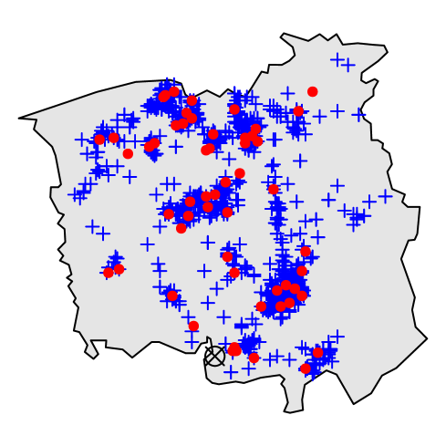
Figure 4: Locations of larynx (red dots) and lung (blue pluses) cancers together with the location of the industrial incinerator (black circle cross).

Figure 5: Geospatial window used for the Chicago Crime experiment. The window coincides with the OpenStreetMap tile at zoom level of 10 that covers the city of Chicago and the surrounding region. Map data copyrighted OpenStreetMap contributors and available from https://www.openstreetmap.org.

Considering the larynx cancer locations as the point pattern $\boldsymbol{X}$ and the lung cancer locations as the pattern $\boldsymbol{Y}$, we would like to test whether the functional form of the intensity is the same for these patterns. Note that the null hypothesis states that there is a constant $c$ such that the intensities of the two point processes satisfy $\lambda^{\mathrm{Larynx}}(\cdot)=c\lambda^{\mathrm{Lung}}(\cdot)$. Applying our methodology, we find the $p$-value of $p^{H}=0.965$ and a mean Bayes factor of $\overline{\mathrm{BF}}_{10}=0.24$, which leads us to retain the null hypothesis. This is in agreement with the re-analyses of this data such as [19] and the recent in-depth study of this dataset [17] within the context of difficulties that arise in estimating relative risk functions.

Replicated Patterns: Chicago Crime

Crime Type	Tuesday	Thursday	Saturday	Tue vs Thu		Tue vs Sat
	#Pts	#Pts	#Pts	$p$-value	$\overline{\mathrm{BF}}_{10}$	$p$-value	$\overline{\mathrm{BF}}_{10}$
Theft	144.7	150.3	148.6	0.125	0.838	0.001	29.503
Battery	88.0	87.2	115.5	0.179	0.682	0.002	12.403
Deceptive Practice	43.0	42.8	36.2	0.825	0.409	0.006	5.728
Criminal Damage	50.5	53.6	61.4	0.566	0.502	0.014	2.799
Robbery	19.9	19.4	22.9	0.099	0.858	0.051	1.231
Narcotics	28.1	27.1	30.1	0.915	0.392	0.613	0.486
Burglary	25.9	25.4	22.8	0.475	0.523	0.657	0.469
Assault	40.3	41.4	37.9	0.987	0.342	0.725	0.435
Other Offense	32.8	31.6	28.1	0.788	0.416	0.968	0.358
Motor Veh Theft	21.1	20.3	22.6	0.997	0.322	0.997	0.322

Table 6: Application of the replicated pattern comparison to Chicago Crime dataset. The entries in bold correspond to the rejected hypotheses with the BH procedure at the FDR level of 0.1.

In this experiment we use the dataset provided by Chicago Data Portal that reflects reported incidents of crime that occurred in the City of Chicago. We consider all of the crimes during the year of 2018 within a geospatial window (shown in Figure 5), and the goal is to compare the spatial patterns of each crime type between weekdays and weekends. We wanted to pick days that are maximally spaced out and avoid ambiguity (e.g. Friday nights), so we decided to compare the following days of the week: Tuesday, Thursday, and Saturday. The comparison between Tuesday and Thursday serves as a sanity check, as we do not expect to see any differences between them.

For each day and type of crime we obtain the crime patterns, and filter by the count of points keeping the patterns that have at least 15 points. Next we count how many distinct patterns are available for each day and type of crime; we found the crime types that had at least 40 patterns for each of Tuesday, Thursday, and Saturday and we kept 40 patterns per each to avoid differences in the testing power. The types of crimes remaining after this filtering are shown in Table 6 together with the average count of points per pattern.

The results of comparisons are shown in the last two columns of Table 6. We run the Benjamini-Hochberg [11] procedure on the 20 resulting $p$-values at the false discovery rate of $0.1$, and the rejected hypotheses are indicated by the $p$-values in bold. As expected, no differences were detected between Tuesday and Thursday patterns. On the other hand, we see that there are statistically significant differences between Tuesday and Saturday patterns in the following categories of crime: theft, battery, deceptive practice, and criminal damage. The corresponding mean Bayes factors can be interpreted using Jeffreys’ rule of thumb [34] for strength of evidence pointing out that there is substantial or strong evidence for the first three differences, whereas the difference in criminal damage “is not worth more than a bare mention”.

7 Conclusion

We have introduced an approach to detect differences in the first-order structure of spatial point patterns. The proposed approach leverages the kernel mean embedding in a novel way, by introducing its approximate version. Hypothesis testing is based on conducting $t$-tests on each dimension of the approximate embedding and combining them using either the harmonic mean or Cauchy approach. Our experiments confirm that the resulting tests are powerful and the $p$-values are well-calibrated. Two applications to real world data have been presented.

A number of possible extensions can be addressed in future research. First, to focus the paper we avoided discussing hypothesis tests to detect differences between more than two single patterns or more than two groups of replicated patterns. Since aKME is based on means, under suitable assumptions we can instead of $t$-tests perform an analysis of variance (ANOVA) F test for differences among means and combine the resulting $p$-values as before. Second, in the experimental section we showed that the single pattern comparison test can be applied even when Poisson assumption is not met; this was based on an intuitive notion of effective sample size. This is different from the one discussed in [26, 49, 1], and it would be interesting to formalize this notion and to provide methods for its reliable estimation. Third avenue for future research would be to leverage the directionality of the projections that correspond to the subsets of dimensions of the aKME (c.f. Figure 1). One can envision a technique where anisotropy in the first-order structure difference would be detected by appropriately combining the $p$-values. An orthogonal aspect would be to investigate the scales at which the differences happen, this time combining the $p$-values for each scale. The harmonic mean approach is suitable for such multi-facet and multi-level analyses as described in [53]. Fourth direction for future work is studying the proposed approach in the context of goodness-of-fit testing of the first-order structure. Since our approach allows for vastly differing numbers of points in the patterns, one can compute a low-variance approximation to the theoretical aKME of the model distribution by constructing a pattern via drawing a large number of points from that distribution; our initial studies gave favorable results when compared to existing techniques such as [27]. Finally, it would be desirable to extend the proposed technique to the high-dimensional setting, where the curse of the dimensionality would be an important factor that can affect the testing power.

Acknowledgements

We are grateful to the revewers for their constructive comments which have led to a much improved version of the article. We thank Alfred Stein for his editorial efforts in handling this article for the Spatial Statistics journal. Finally, we thank Tonglin Zhang and Isabel Fuentes-Santos for providing the source code of the methods from their respective papers.

Appendix A Proof of Consistency

							Harmonic						Adjusted Harmonic
Model	$\beta_{1}$	$\beta_{2}$	$\lambda$				$\alpha=0.01$	$\alpha=0.05$	$\alpha=0.1$				$\alpha=0.01$	$\alpha=0.05$	$\alpha=0.1$
Size
Linear	1	1	100				0.008	0.058	0.108				0.010	0.060	0.105
		1	400				0.009	0.045	0.098				0.007	0.038	0.085
		1	800				0.008	0.050	0.104				0.006	0.048	0.093
	2	2	100				0.011	0.054	0.106				0.013	0.048	0.104
		2	400				0.008	0.052	0.099				0.008	0.055	0.101
		2	800				0.010	0.044	0.090				0.008	0.042	0.094
	3	3	100				0.010	0.042	0.090				0.008	0.044	0.087
		3	400				0.012	0.058	0.106				0.010	0.049	0.104
		3	800				0.012	0.048	0.088				0.010	0.044	0.084
Sine	1	1	100				0.010	0.054	0.100				0.008	0.058	0.100
		1	400				0.014	0.047	0.102				0.014	0.045	0.102
		1	800				0.012	0.059	0.106				0.008	0.058	0.112
	2	2	100				0.013	0.057	0.096				0.010	0.056	0.102
		2	400				0.014	0.058	0.094				0.012	0.056	0.093
		2	800				0.008	0.046	0.095				0.007	0.042	0.094
	3	3	100				0.008	0.044	0.092				0.010	0.050	0.098
		3	400				0.008	0.051	0.090				0.006	0.046	0.093
		3	800				0.010	0.046	0.091				0.012	0.048	0.091
Power
Linear	1	2	100				0.085	0.206	0.310				0.086	0.198	0.300
		2	400				0.644	0.816	0.882				0.627	0.818	0.879
		2	800				0.972	0.992	0.996				0.962	0.990	0.995
		3	100				0.587	0.762	0.848				0.538	0.756	0.852
		3	400				1.000	1.000	1.000				1.000	1.000	1.000
		3	800				1.000	1.000	1.000				1.000	1.000	1.000
	2	3	100				0.070	0.179	0.274				0.058	0.182	0.270
		3	400				0.520	0.725	0.808				0.496	0.718	0.815
		3	800				0.915	0.968	0.982				0.912	0.968	0.981
Sine	1	2	100				0.352	0.608	0.720				0.338	0.564	0.710
		2	400				0.997	0.999	1.000				0.998	0.999	1.000
		2	800				1.000	1.000	1.000				1.000	1.000	1.000
		3	100				0.942	0.985	0.990				0.940	0.982	0.992
		3	400				1.000	1.000	1.000				1.000	1.000	1.000
		3	800				1.000	1.000	1.000				1.000	1.000	1.000
	2	3	100				0.050	0.190	0.308				0.034	0.144	0.256
		3	400				0.768	0.912	0.942				0.784	0.912	0.943
		3	800				0.994	1.000	1.000				0.994	0.999	1.000

Table 7: Comparison of rejection rates for the single pattern comparison test between harmonic and adjusted harmonic approaches.

Here we provide the proof of consistency of the proposed test for single pattern comparison with increasing number of points in the patterns. A similar argument applies to the replicated pattern comparison test with the increasing number of replications; this, of course, assumes that the condition of Eq. (4.2) holds.

Consider two density functions $p(\cdot)\neq q(\cdot)$ and the corresponding inhomogeneous Poisson point processes $P$ and $Q$ such that $\lambda^{P}(\cdot)=Np(\cdot)$ and $\lambda^{Q}(\cdot)=Nq(\cdot)$. We will first show that there exists $D=2m_{0}\ell_{0}$ dimensional aKME embedding based test such that for any size $\alpha$, we have $\mathrm{Prob}(\mathrm{reject}\,H_{0})\to 1$ when $N\to\infty$. Afterwards, we will discuss how to modify our test and slowly increase $D$ with $N$ so as to obtain general consistency.

As discussed in Section 3, we have the following connection to MMD,

$$\|\mu_{m,\ell}^{p}-\mu_{m,\ell}^{q}\|^{2}\to MMD^{2}(p,q),$$

with increasing quality of quadrature approximation as $m,\ell\to\infty$. For a large class of density functions, $p(\cdot)\neq q(\cdot)$ implies $MMD^{2}(p,q)>0$ [25]. As a result, there exist $m_{0}$ and $\ell_{0}$ such that the $D=2m_{0}\ell_{0}$ dimensional aKME satisfies $\|\mu_{m_{0},\ell_{0}}^{p}-\mu_{m_{0},\ell_{0}}^{q}\|^{2}>0$. Thus, there is a dimension $k$ in the embedding space such that $1\leq k\leq D$ and aKME embeddings disagree on this dimension: $(\mu_{m_{0},\ell_{0}}^{p})_{k}\neq(\mu_{m_{0},\ell_{0}}^{q})_{k}$. Note that the value of $D$ depends only on $p$ and $q$, but not on $N$.

Of course, the difference in the $k$-th dimension will be discerned by the $t$-test as $N\to\infty$: we will have the corresponding $p$-value $p_{k}\to 0$. More precisely, for any $\delta>0$, $\mathrm{Prob}(p_{k}<\delta)\to 1.$ If we were to use Bonferroni correction instead of combining $p$-values, we would get for a test size $\alpha,$ the following $\mathrm{Prob}(\mathrm{reject}\,H_{0})=\mathrm{Prob}(p_{k}<\alpha/D)\to 1$ as $N\to\infty$. We will see that both harmonic mean combination and Cauchy combination tests are asymptotically equivalent to Bonferroni correction in the worst-case regime, yielding consistency.

We first prove consistency for the $p^{H}$ based test. In addition to $p_{k}$ we have $D-1$ other $p$-values coming from testing the remaining coordinates of the embedding. To consider the worst-case scenario, assume that the null holds for all of these $D-1$ coordinates. For the harmonic mean combination, the combined $p$-value can be upper-bounded by substituting the null $p$-values by 1. Plugging in $p_{i}=1,i\neq k$ we get,

$$p^{H}\leq H\left(\frac{D}{D-1+\frac{1}{p_{k}}}\right)=H\left(\frac{Dp_{k}}{1+(D-1)p_{k}}\right)\sim H(Dp_{k})\sim Dp_{k},$$

for small $p_{k}$; here we used $\lim_{x\to 0}H(x)/x\to 1$. This proves that as $N\to\infty$, $\mathrm{Prob}(\mathrm{reject}\,H_{0})=\mathrm{Prob}(p^{H}<\alpha)\geq\mathrm{Prob}(Dp_{k}<\alpha)=\mathrm{Prob}(p_{k}<\alpha/D)\to 1$ for any level $\alpha>0$.

To carry out a similar limit argument for the Cauchy combination test, more care is needed to avoid the singularity around $p$-values close to 1. Using approximation by normal distribution and the commonly used bounds on the tail area, one can show that for the non-null $t$-test the $p$-values is of the order $p_{k}\sim e^{-\theta N}/\sqrt{N}$ for some $\theta$ that depends on the effect size; so, we have $\mathrm{Prob}(p_{k}<e^{-\theta N})\to 1$. Take an arbitrary sequence $\epsilon_{N}\to 0$ such that the convergence happens slower than $p_{k}\to 0$ with $N\to\infty$, e.g. $\epsilon_{N}=1/N^{r}$ for any positive $r$ would work. Considering the worst-case scenario above, we have that with probability $(1-\epsilon_{N})^{D-1}$ the following holds: $p_{i}\leq 1-\epsilon_{N}$ $\forall i\neq k$; this stems from the uniform distribution of $p$-values under the null. Now to obtain an upper bound for the Cauchy combination $p$-value $p^{C}$ we can replace all of the null $p$-values with $1-\epsilon_{N}$, yielding with at least probability of $(1-\epsilon_{N})^{D-1}$:

$$\cot\pi p^{C}\geq\frac{(D-1)\cot\pi(1-\epsilon_{N})+\cot\pi p_{k}}{D}\sim\frac{1}{D\pi}(p_{k}^{-1}-(D-1)\epsilon_{N}^{-1})\sim\frac{1}{D\pi}e^{\theta N},$$

using simple asymptotics for the cotangent function and by the assumption on $\epsilon_{N}$. The inequality implies smallness of $p^{C}$which allows us to use the asymptotic $\cot x\sim 1/x$ once again to get

$$\mathrm{Prob}(p^{C}\leq De^{-\theta N})\geq(1-\epsilon_{N})^{D-1},$$

in other words, Cauchy combination test is asymptotically equivalent to Bonferroni correction in this regime. With $N\to\infty$ we have $p^{C}\to 0$ with probability $(1-\epsilon_{N})^{D-1}\to 1$, proving consistency for the Cauchy version of our test.

The above argument assumes the knowledge of $D=m_{0}\ell_{0}$ when conducting the test. To avoid this assumption, we need to increase the dimensionality of aKME with $N$. To this end, consider two sequences of integers that satisfy $m_{N}\to\infty$ and $\ell_{N}\to\infty$ as $N\to\infty$, potentially with repeating terms (e.g. they can sweep all the pairwise combinations of integers $m$ and $\ell$). We define $\mathrm{aKME}_{N}$ as the concatenation of all unique $\mathrm{aKME}_{m_{s},\ell_{s}}$, $s\leq N$ and apply the $t$-tests to each dimension of $\mathrm{aKME}_{N}$. Denote the dimensionality of this overall embedding as $D_{N}$. As $N\to\infty$, we are guaranteed to include a non-null dimension into the overall $\mathrm{aKME}_{N}$ and it will stay in due to the nestedness of this construction. As explained above we can use Bonferroni correction as a surrogate for both of the combination techniques. Thus, concentrating on Bonferroni correction, we have $\mathrm{Prob}(\mathrm{reject}\,H_{0})=\mathrm{Prob}(p_{k}<\alpha/D_{N})$. Since $\mathrm{Prob}(p_{k}<e^{-\theta N})\to 1$, we see that if, for example, $D_{N}$ grows polynomially (which is easy to attain) consistency will follow. For the Cauchy combination test one has to be slightly more careful and select $\epsilon_{N}$ in the previous paragraph that goes to zero faster than, say, $1/D_{N}^{2}$.

Appendix B Implementation of Single Pattern Comparison in R

Here we provide an R implementation of the single pattern comparison test for the example demonstrated in Section 6.2, namely comparison of the larynx and lung cancer location patterns.

⬇

library(spatstat)

library(harmonicmeanp)

library(BayesFactor)

radialGaussHermiteData <- function(k) {

if (k == 4) {

Roots4 = c(

0.3961205684809970482046989062,

1.1767346714185921750900701015,

2.2010676629189581946543092946,

3.4836109980286615716953100856

)

Weights4 = c(

0.2279981086730596270303131898,

0.538464759426994159094177725,

0.2215779133653168055615931299,

0.0119592185346294083139159552

)

list(x = Roots4, w = Weights4)

} else {

stop(

"Please refer to the values in

http://www.jaeckel.org/RootsAndWeightsForRadialGaussHermiteQuadrature.cpp"

)

}

}

#maps every point in the point pattern using aKME process

get_aKME <- function(p, sigmas, n_radial = 4, n_linear = 4) {

#radial unit vectors

theta = seq(0, pi, length.out = n_radial + 1)[-(n_radial + 1)]

W0 = cbind(cos(theta), sin(theta))

#quadrature roots and weights

temp = radialGaussHermiteData(n_linear)

Roots = temp$x

Weights = temp$w

W = do.call(’rbind’, lapply(seq_along(Roots), function(i) Roots[i] * W0))

coeff = rep(sqrt(Weights / n_radial), each=nrow(W0))

#project the points onto the lines, c.f. Figure 1

proj = W%*%rbind(p$x, p$y)

#embedding: for each sigma wrap on the circle of corresponding radius

emb = lapply(seq_along(sigmas), function(i)

t(rbind(cos(proj / sigmas[i]) * coeff, sin(proj / sigmas[i]) * coeff)))

#concatenated embedding, one row for each point of the pattern

#dim = (#points, #sigmas x 2 x # n_radial x n_linear)

do.call(’cbind’, emb)

}

#load data

d = chorley

d1 = split(d)$lung

d2 = split(d)$larynx

#we use several Gaussian widths at once

#these values are for [0,1]x[0,1] window

sigma_list0 = c(1 / 16, 1 / 8, 1 / 4)

sigma_list = diameter(Window(d)) * sigma_list0 / sqrt(2)

aKME1 = get_aKME(d1, sigma_list)

aKME2 = get_aKME(d2, sigma_list)

#p-values for t-tests on each dimension of the embeddings

p_ttests = sapply(seq_len(ncol(aKME1)), function(i)

t.test(aKME1[, i], aKME2[, i])$p.value)

#overall p-value using harmonic mean combo

p_harmonic = p.hmp(p_ttests, L = length(p_ttests), multilevel=FALSE)

#0.9654329

#overall p-value using Cauchy combo

p_cauchy = 0.5 - atan(mean(tan((0.5-p_ttests)*pi)))/pi

#0.6727789

#mean Bayes factor

bf10_mean = mean(sapply(seq_len(ncol(aKME1)), function(i)

extractBF(ttestBF(aKME1[, i], aKME2[, i]))$bf))

#0.2443478

chorley_code.R

References

- [1] Jonathan Acosta, Ronny Vallejos, and Daniel Griffth. On the effective geographic sample size. Journal of Statistical Computation and Simulation, 88(10):1958–1975, 2018.
- [2] M.V. Alba-Fernández, F.J. Ariza-López, M. Dolores Jiménez-Gamero, and J. Rodríguez-Avi. On the similarity analysis of spatial patterns. Spatial Statistics, 18:352 – 362, 2016.
- [3] N.H. Anderson, P. Hall, and D.M. Titterington. Two-sample test statistics for measuring discrepancies between two multivariate probability density functions using kernel-based density estimates. Journal of Multivariate Analysis, 50(1):41 – 54, 1994.
- [4] Martin A. Andresen. Testing for similarity in area-based spatial patterns: A nonparametric monte carlo approach. Applied Geography, 29(3):333 – 345, 2009.
- [5] Ery Arias-Castro and Shiyun Chen. Distribution-free multiple testing. Electronic Journal of Statistics, 11(1):1983–2001, 2017.
- [6] Haim Avron, Vikas Sindhwani, Jiyan Yang, and Michael W. Mahoney. Quasi-Monte Carlo feature maps for shift-invariant kernels. Journal of Machine Learning Research, 17(120):1–38, 2016.
- [7] Adrian Baddeley, Ege Rubak, and Rolf Turner. Spatial Point Patterns: Methodology and Applications with R. Chapman and Hall/CRC Press, London, 2015.
- [8] Rina Foygel Barber and Emmanuel J. Candés. Controlling the false discovery rate via knockoffs. The Annals of Statistics, 43(5):2055–2085, 10 2015.
- [9] L. Baringhaus and C. Franz. On a new multivariate two-sample test. Journal of Multivariate Analysis, 88(1):190 – 206, 2004.
- [10] Robert Bartoszynski, Barry W. Brown, Charles M. McBride, and James R. Thompson. Some nonparametric techniques for estimating the intensity function of a cancer related nonstationary poisson process. The Annals of Statistics, 9(5):1050–1060, 09 1981.
- [11] Yoav Benjamini and Yosef Hochberg. Controlling the false discovery rate: A practical and powerful approach to multiple testing. Journal of the Royal Statistical Society. Series B (Methodological), 57(1):289–300, 1995.
- [12] Patrick Billingsley. Probability and measure. Wiley, New York, third edition, 1995.
- [13] Song Xi Chen and Ying-Li Qin. A two-sample test for high-dimensional data with applications to gene-set testing. Annals of Statistics, 38(2):808–835, 04 2010.
- [14] T. M. Cover. Geometrical and statistical properties of systems of linear inequalities with applications in pattern recognition. IEEE Transactions on Electronic Computers, EC-14(3):326–334, June 1965.
- [15] Lionel Cucala. Two-dimensional spacings and noisy observations in the analysis of spatial point patterns. Theses, Université des Sciences Sociales - Toulouse I, December 2006.
- [16] Tilman M. Davies and Martin L. Hazelton. Adaptive kernel estimation of spatial relative risk. Statistics in Medicine, 29(23):2423–2437, 2010.
- [17] Tilman M. Davies, Khair Jones, and Martin L. Hazelton. Symmetric adaptive smoothing regimens for estimation of the spatial relative risk function. Computational Statistics & Data Analysis, 101:12 – 28, 2016.
- [18] Peter J. Diggle. A point process modelling approach to raised incidence of a rare phenomenon in the vicinity of a prespecified point. Journal of the Royal Statistical Society. Series A (Statistics in Society), 153(3):349–362, 1990.
- [19] Peter J. Diggle, Nicholas Lange, and Francine M. Benes. Analysis of variance for replicated spatial point patterns in clinical neuroanatomy. Journal of the American Statistical Association, 86(415):618–625, 1991.
- [20] Tarn Duong, Bruno Goud, and Kristine Schauer. Closed-form density-based framework for automatic detection of cellular morphology changes. Proceedings of the National Academy of Sciences, 109(22):8382–8387, 2012.
- [21] Moulines Eric, Francis R. Bach, and Zaïd Harchaoui. Testing for homogeneity with kernel Fisher discriminant analysis. In International Conference on Neural Information Processing Systems, NIPS, pages 609–616. 2008.
- [22] Seth Flaxman, Yee Whye Teh, and Dino Sejdinovic. Poisson intensity estimation with reproducing kernels. Electronic Journal of Statistics, 11(2):5081–5104, 2017.
- [23] I. Fuentes-Santos, W. González-Manteiga, and J. Mateu. A nonparametric test for the comparison of first-order structures of spatial point processes. Spatial Statistics, 22:240 – 260, 2017.
- [24] I. J. Good. Significance tests in parallel and in series. Journal of the American Statistical Association, 53(284):799–813, 1958.
- [25] Arthur Gretton, Karsten M. Borgwardt, Malte J. Rasch, Bernhard Schölkopf, and Alexander Smola. A kernel two-sample test. J. Mach. Learn. Res., 13:723–773, March 2012.
- [26] Daniel A. Griffith. Effective geographic sample size in the presence of spatial autocorrelation. Annals of the Association of American Geographers, 95(4):740–760, 2005.
- [27] Yongtao Guan. A goodness-of-fit test for inhomogeneous spatial poisson processes. Biometrika, 95(4):831–845, 2008.
- [28] Ute Hahn. A studentized permutation test for the comparison of spatial point patterns. Journal of the American Statistical Association, 107(498):754–764, 2012.
- [29] Peter Hall. Resampling a coverage pattern. Stochastic Processes and their Applications, 20(2):231 – 246, 1985.
- [30] Z. Harchaoui, F. Bach, O. Cappe, and E. Moulines. Kernel-based methods for hypothesis testing: A unified view. IEEE Signal Processing Magazine, 30(4):87–97, July 2013.
- [31] Trevor J. Hastie, Robert John Tibshirani, and Jerome H. Friedman. The elements of statistical learning : data mining, inference, and prediction. Springer series in statistics. Springer, New York, 2009.
- [32] N A Heard and P Rubin-Delanchy. Choosing between methods of combining -values. Biometrika, 105(1):239–246, 01 2018.
- [33] Peter Jaeckel. A Note on Multivariate Gauss-Hermite Quadrature. Technical report, London: ABN-Amro., May 2005.
- [34] H. Jeffreys. Theory of Probability. Oxford, Oxford, England, third edition, 1961.
- [35] Wittawat Jitkrittum, Wenkai Xu, Zoltan Szabo, Kenji Fukumizu, and Arthur Gretton. A linear-time kernel goodness-of-fit test. In International Conference on Neural Information Processing Systems, NIPS, pages 262–271, 2017.
- [36] Robert E. Kass and Adrian E. Raftery. Bayes factors. Journal of the American Statistical Association, 90(430):773–795, 1995.
- [37] Julia E. Kelsall and Peter J. Diggle. Kernel estimation of relative risk. Bernoulli, 1(1/2):3–16, 1995.
- [38] Julia E. Kelsall and Peter J. Diggle. Non-parametric estimation of spatial variation in relative risk. Statistics in Medicine, 14(21 - 22):2335–2342, 1995.
- [39] Yaowu Liu and Jun Xie. Cauchy combination test: A powerful test with analytic p-value calculation under arbitrary dependency structures. Journal of the American Statistical Association, 115(529):393–402, 2020.
- [40] Thomas M. Loughin. A systematic comparison of methods for combining p-values from independent tests. Computational Statistics & Data Analysis, 47(3):467 – 485, 2004.
- [41] Krikamol Muandet, Kenji Fukumizu, Bharath Sriperumbudur, and Bernhard Schölkopf. Kernel mean embedding of distributions: A review and beyond. Foundations and Trends in Machine Learning, 10(1-2):1–141, 2017.
- [42] Marina Munkhoeva, Yermek Kapushev, Evgeny Burnaev, and Ivan Oseledets. Quadrature-based features for kernel approximation. In International Conference on Neural Information Processing Systems, NIPS, pages 9147–9156. 2018.
- [43] Ali Rahimi and Benjamin Recht. Random features for large-scale kernel machines. In International Conference on Neural Information Processing Systems, NIPS, pages 1177–1184, 2007.
- [44] B. D. Ripley. The second-order analysis of stationary point processes. Journal of Applied Probability, 13(2):255–266, 1976.
- [45] Jeffrey N. Rouder, Paul L. Speckman, Dongchu Sun, Richard D. Morey, and Geoffrey Iverson. Bayesian t tests for accepting and rejecting the null hypothesis. Psychonomic Bulletin & Review, 16(2):225–237, 2009.
- [46] B. W. Silverman. On the estimation of a probability density function by the maximum penalized likelihood method. The Annals of Statistics, 10(3):795–810, 09 1982.
- [47] J. Stoer and Roland Bulirsch. Introduction to numerical analysis (Third edition). Texts in Applied Mathematics. 2002.
- [48] Gábor J. Székely and Maria L. Rizzo. A new test for multivariate normality. Journal of Multivariate Analysis, 93(1):58 – 80, 2005.
- [49] Ronny Vallejos and Felipe Osorio. Effective sample size of spatial process models. Spatial Statistics, 9:66 – 92, 2014.
- [50] Vladimir Vovk and Ruodu Wang. Combining e-values and p-values. To appear in Biometrika, 2019.
- [51] Vladimir Vovk and Ruodu Wang. Combining e-values and p-values. arXiv e-prints, page arXiv:1912.06116, December 2019.
- [52] Rasmus Plenge Waagepetersen. An estimating function approach to inference for inhomogeneous Neyman-Scott processes. Biometrics, 63(1):252–258, 2007.
- [53] Daniel J. Wilson. The harmonic mean p-value for combining dependent tests. Proceedings of the National Academy of Sciences, 116(4):1195–1200, 2019.
- [54] Makoto Yamada, Denny Wu, Yao-Hung Hubert Tsai, Hirofumi Ohta, Ruslan Salakhutdinov, Ichiro Takeuchi, and Kenji Fukumizu. Post selection inference with incomplete maximum mean discrepancy estimator. In International Conference on Learning Representations, 2019.
- [55] Jiasen Yang, Vinayak Rao, and Jennifer Neville. A Stein-Papangelou goodness-of-fit test for point processes. In International Conference on Artificial Intelligence and Statistics, AISTATS, 2019.
- [56] Felix Xinnan Yu, Ananda Theertha Suresh, Krzysztof Choromanski, Daniel Holtmann-Rice, and Sanjiv Kumar. Orthogonal random features. In International Conference on Neural Information Processing Systems, NIPS, pages 1983–1991, 2016.
- [57] Tonglin Zhang and Run Zhuang. Testing proportionality between the first-order intensity functions of spatial point processes. Journal of Multivariate Analysis, 155:72 – 82, 2017.
- [58] Ji Zhao and Deyu Meng. Fastmmd: Ensemble of circular discrepancy for efficient two-sample test. Neural Computation, 27(6):1345–1372, June 2015.
- [59] A. A. Zinger, A. V. Kakosyan, and L. B. Klebanov. A characterization of distributions by mean values of statistics and certain probabilistic metrics. Journal of Soviet Mathematics, 59(4):914–920, 1992.