Current noise geometrically generated by a driven magnet

Abstract

We consider a non-equilibrium cross-response phenomenon, whereby a driven magnetization gives rise to electric shot noise (but no d.c. current). This effect is realized on a nano-scale, with a small metallic ferromagnet which is tunnel-coupled to two normal metal leads. The driving gives rise to a precessing magnetization. The geometrically generated noise is related to a non-equilibrium distribution in the ferromagnet. Our protocol provides a new channel for detecting and characterizing ferromagnetic resonance.

Off-diagonal (cross-) response phenomena, e.g. the thermoelectric effect, are ubiquitous in physics. In spintronic systems, by applying an electric charge current one can drive magnetization dynamics and vice versa Slonczewski (1996); Berger (1996, 1999); Tserkovnyak et al. (2002); Brataas et al. (2002); Tserkovnyak et al. (2005, 2008). This usually requires magnetic contacts which allow for a conversion between spin and charge currents; see however Jonson et al. (2019). In this Letter we report a higher order strongly non-equilibrium cross-response effect. Namely, we show that by driving magnetization dynamics one can generate electric shot noise Landauer (1998); Blanter and Büttiker (2000) without generating charge current. Strikingly, no magnetic leads are needed and the leads can be at equilibrium with each other.

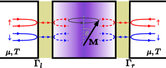
Figure 1: A small metallic ferromagnet with precessing magnetization is tunnel-coupled to two normal metal leads, which are at equilibrium with each other. The precessing magnetization pumps a spin-current from the small ferromagnet into the leads Tserkovnyak et al. (2002); Brataas et al. (2002); Tserkovnyak et al. (2005). The average charge current vanishes by symmetry. Thus, the current of spin-up electrons and spin-down electrons balance each other on average and in each junction separately; in the ferromagnet, the precessing magnetization mixes spin-up and spin-down electrons. All four spin-resolved electron currents are fluctuating. These fluctuations combine to give rise to the noise of left to right (transport) charge current.

We consider a small metallic ferromagnet with magnetization driven to precess. The ferromagnet is tunnel-coupled to two normal metal leads; see Fig. 1. The precessing magnetization drives the electrons of the ferromagnet into a strongly non-equilibrium state. This effect is most pronounced if the ferromagnet is small enough such that internal relaxation is negligible compared to the relaxation due to the coupling to the leads. The precessing magnetization, in turn, induces non-equilibrium shot noise of the electric current. The non-equilibrium distribution responsible for the shot noise is governed by the geometric Berry phase due to precessing magnetization, branding the shot noise geometric. This shot noise exists even when both leads are in equilibrium with each other, although the average charge current vanishes then.

Shot noise is particularly interesting in spintronics because it gives insights into the magnetic configuration and its dynamics which may be hard to obtain otherwise Foros et al. (2009); Arakawa et al. (2015); Kamra and Belzig (2016a, b); Cascales et al. (2015); Virtanen and Heikkilä (2017); Horovitz and Golub (2019).

Results.—In order to describe dynamics of the magnetization of a small ferromagnet we use the macrospin approximation, i.e., the magnetization is given by a single vector $\bm{M}=M(\sin\theta\cos\phi,\sin\theta\sin\phi,\cos\theta)$. We assume a steady state precession of the magnetization at a constant polar angle $\theta$ and with a constant precession frequency $\dot{\varphi}$. Under this assumptions, we found that the charge current vanishes on average, $I=0$, but the current noise remains finite:

$$S=4g_{t}T+g_{t}\sin^{2}\theta\,\Big{(}\dot{\phi}\,\coth{\frac{\dot{\phi}}{2T}}-2T\Big{)}\ .$$ (1)

Here $g_{t}=2(\rho_{\uparrow}+\rho_{\downarrow})\Gamma_{l}\Gamma_{r}/(\Gamma_{l}+\Gamma_{r})$ is the total conductance of the double tunnel-junction with spin-dependent density of states of the small ferromagnet $\rho_{\sigma}$. The rates $\Gamma_{l}$ and $\Gamma_{r}$ characterize the spin-conserved tunneling to left and right leads respectively. The precessing magnetization pumps a spin-current into the adjacent leads Tserkovnyak et al. (2002); Brataas et al. (2002); Tserkovnyak et al. (2005), which drives the electron system into a strong non-equilibrium state Ludwig et al. (2017, 2019); see Fig. 3. At high temperatures $(T\gg\dot{\phi})$, the noise is dominated by the first term $S\approx 4g_{t}T$, which is the standard thermal noise. At low temperatures $(T\ll\dot{\phi}\,\sin^{2}\theta)$, however, the noise is dominated by the second term $S\approx g_{t}\sin^{2}\theta\,|\dot{\phi}|$. The time-dependence of the magnetization is the source of driving for the electron system. Therefore, the precession frequency $\dot{\phi}$ acts like a voltage bias for standard shot noise.

Application to FMR-driven magnet.—Now let us consider our setup under conditions of a ferromagnetic resonance (FMR). The dynamics of the magnetization is phenomenologically described by the Landau-Lifshitz-Gilbert equation $\bm{\dot{m}}=\bm{m}\times\bm{B}-\alpha\,\bm{m}\times\bm{\dot{m}}$, where $\bm{m}=\bm{M}/M$ is the direction of the magnetization and $\alpha$ is the Gilbert-damping coefficient. For the FMR-setup, we choose the magnetic field $\bm{B}=(\Omega\cos\omega_{d}t,\Omega\sin\omega_{d}t,B_{0})$ with a fixed component $B_{0}$ in $z-$direction and, perpendicular to it, a small driving field with strength $\Omega$ and frequency $\omega_{d}$. For negligible internal relaxation, the damping is dominated by the coupling to the leads. Without driving, the Gilbert-damping would relax the magnetization towards $\theta=0$. With driving ($\Omega\neq 0$), however, the magnetization can be brought into a steady state precession. That is, after the decay of transient effects, the magnetization precesses at the frequency of the driving field $\dot{\phi}=\omega_{d}$ and the polar angle $\theta$ is determined by the competition between Gilbert-damping and FMR-driving. Explicitly, $\theta$ is determined by

$$\sin^{2}\theta=\frac{(\Omega_{+}+\Omega_{-})^{2}}{\Omega^{2}_{+}+\Omega^{2}_{-}+2\Delta^{2}+2\sqrt{(\Delta^{2}+\Omega_{+}^{2})(\Delta^{2}+\Omega_{-}^{2})}}\ ,$$ (2)

with $\Omega_{\pm}=\Omega\pm\alpha\omega_{d}$ and the detuning parameter $\Delta=\omega_{d}+B_{0}$. The dependence of $\sin^{2}\theta$ on precession frequency $\omega_{d}$ has a resonant character with a maximum at $\omega_{d}=-B_{0}$. This ferromagnetic resonance of the magnetization’s steady state precession directly translates into a resonance in the current noise; see Fig. 2. At low temperatures, $T\ll\omega_{d}\sin^{2}\theta$, the form of the resonance in the current noise resembles the FMR structure of the stationary precession angle. At higher temperatures, the resonance in the current noise can be visible on top of the constant thermal noise. Now we explain how our results were derived.

Figure 2: When the steady state precession of the magnetization is maintained by driving with a FMR-setup, the polar angle $\theta$ depends on driving frequency $\dot{\phi}=\omega_{d}$. The peak of $\sin^{2}\theta$ at $\omega_{d}=-B_{0}$ ($\Delta=0$) is a typical FMR-peak. We show the zero-frequency noise of charge current that is generated by the precessing magnetization; we subtract the thermal contribution and normalize onto the value of the total conductance, that is, we show $(S-4g_{t}T)/g_{t}$. The generated noise of charge current clearly reflects the peak structure of $\sin^{2}\theta$ in the FMR-setup. Parameters in figure: $\alpha=0.04$, $\Omega/(\alpha B_{0})=0.63$.

The effective action.—Because the dynamics of the magnetization creates non-equilibrium conditions, we apply Keldysh formalism Kamenev (2011); Kamenev and Levchenko (2009); Altland and Simons (2010). The Keldysh generating function is $\mathcal{Z}=\int D[\bar{\Psi},\Psi]\,\exp{(i\mathcal{S})}$ with the action,

$$\mathcal{S}=\oint_{K}\!\!dt\ \bar{\Psi}\,(i\partial_{t}-h_{s}-\hat{\Sigma})\,\Psi\ ,$$ (3)

where the integral is along the Keldysh contour and $\Psi,\bar{\Psi}$ denote the fermionic fields of the small ferromagnet. The self-energy operator $\hat{\Sigma}$ is defined by $[\hat{\Sigma}\Psi](t)=\oint dt^{\prime}\,\Sigma(t-t^{\prime})\Psi(t^{\prime})$, where $\Sigma=\Sigma_{l}+\Sigma_{r}$ is the self-energy arising from the tunnel-coupling to the left lead $\Sigma_{l}$ and right lead $\Sigma_{r}$. The self-energy contains the essential information about the tunnel-coupling to the leads: first, the retarded and advanced part contain the tunneling-rates $\Sigma^{R/A}_{l/r}(\omega)=\mp i\Gamma_{l/r}$; second, the Keldysh part contains the distribution functions of the leads $\Sigma^{K}_{l/r}(\omega)=-2i\Gamma_{l/r}F_{l/r}(\omega)$, where $F_{l/r}(\omega)=1-2f_{l/r}(\omega)$ with the Fermi-distributions $f_{l/r}(\omega)=1/[\exp[(\omega-\mu)/T]+1]$. We emphasize that the ferromagnet’s distribution function $f_{s}$, respectively $F_{s}$, is not yet known explicitly but it is implicitly determined by the action, Eq. (3). This distribution function is governed by the coupling to the leads and the dynamics of the magnetization which enters through the effective single-particle Hamiltonian,

$$h_{s}=h_{0}-\bm{M}\bm{\sigma}/2\,$$ (4)

where $\bm{\sigma}$ is the vector of Pauli-matrices and $h_{0}$ is a spin-degenerate single-particle Hamiltonian of the small ferromagnet. For the derivation of the charge noise, the magnetization is considered to be a classical field with given dynamics (steady state precession).

The charge current and its noise are determined with help of a counting field $\lambda$, which is introduced into the self-energy related to the left lead $\Sigma_{l}\rightarrow\Sigma_{l}(\lambda)$. We follow Ref. Virtanen and Heikkilä (2017), and introduce $\lambda$ such that the charge transported through the left junction is determined as $\left\langle Q_{l}\right\rangle=i\partial_{\lambda}\left.\mathcal{Z}(\lambda)\right|_{\lambda=0}$ with the corresponding noise $\left\langle Q_{l}^{2}\right\rangle=(i\partial_{\lambda})^{2}\left.\mathcal{Z}(\lambda)\right|_{\lambda=0}$; details are provided in supplementary material (SM). We can now integrate out the fermions to obtain $\mathcal{Z}(\lambda)=\exp[i\mathcal{S}(\lambda)]$ with the action

$$i\mathcal{S}(\lambda)=\mathrm{tr}\,\mathrm{ln}\big{[}i\partial_{t}-h_{0}+\bm{M}\bm{\sigma}/2-\Sigma(\lambda)\big{]}\ .$$ (5)

The magnetization’s time-dependence makes it complicated to proceed. It is, thus, very convenient to transform to a frame of reference in which the magnetization is time-independent.

Rotating frame.—The magnetization is rotated onto the $z$-axis at all times,

$$R^{\dagger}\bm{M}\bm{\sigma}R=M\sigma_{z}\ ,$$ (6)

with a time-dependent rotation in spin-space $R$. While simplifying the magnetic part, this rotation also comes at a cost: because of its time-dependence, it gives rise to a new term $iR^{\dagger}\dot{R}$ under the $\mathrm{tr}\,\mathrm{ln}$, see Eq. (5), and also rotates the self-energy $R^{\dagger}\Sigma R$. After rotation, the action becomes

$$i\mathcal{S}(\lambda)=\mathrm{tr}\,\mathrm{ln}\big{[}\underbrace{i\partial_{t}-h_{0}+M\sigma_{z}/2+iR^{\dagger}\dot{R}-R^{\dagger}\Sigma(\lambda)R}_{=:\tilde{G}^{-1}_{\lambda}}\big{]}\ ,$$ (7)

where $\tilde{G}^{-1}_{\lambda}$ defined the rotating-frame Green’s function $\tilde{G}_{\lambda}$. Following Ref. Shnirman et al. (2015), we choose the Euler-angle representation $R=e^{-i\frac{\phi}{2}\sigma_{z}}e^{-i\frac{\theta}{2}\sigma_{y}}e^{i\frac{\phi-\chi}{2}\sigma_{z}}$, where $\phi,\theta$ are the angles characterizing the magnetization and the gauge-freedom $\chi$ is fixed by $\dot{\chi}=\dot{\phi}(1-\cos\theta)$. This choice eliminates the spin-diagonal part of $iR^{\dagger}\dot{R}$ which contains information about the Berry phase. However, the Berry phase is not eliminated; instead it is shifted to the rotated self-energy.

Rotating-frame distribution functions.—Because retarded and advanced parts of the self-energy are trivial in spin-space and local in time, the rotation only affects the Keldysh part. While the Keldysh part $\Sigma^{K}(t-t^{\prime})=-2i[\Gamma_{l}F_{l}(t-t^{\prime})+\Gamma_{r}F_{r}(t-t^{\prime})]$ is also trivial in spin-space, it is non-local in time because of the distribution functions $F_{l/r}(t-t^{\prime})$. It follows, $R^{\dagger}(t)\Sigma^{K}(t-t^{\prime})R(t^{\prime})=-2i[\Gamma_{l}\tilde{F}_{l}(t,t^{\prime})+\Gamma_{r}\tilde{F}_{r}(t,t^{\prime})]$ with the rotating-frame distribution functions $\tilde{F}_{l/r}(t,t^{\prime})=R^{\dagger}(t)F_{l/r}(t-t^{\prime})R(t^{\prime})$. For the following, it is convenient to change to the Wigner time-coordinates $\bar{t}=(t+t^{\prime})/2$, $\Delta t=t-t^{\prime}$ and to perform a Fourier-transformation $\Delta t\rightarrow\omega$. For steady state precessions (with $\theta$ and $\dot{\phi}$ constant), the spin-diagonal parts of the rotating-frame distribution functions are given by $\tilde{F}_{l/r}^{\sigma}(\omega)=[\tilde{F}_{l/r}(\omega)]_{\sigma\sigma}=\cos^{2}\frac{\theta}{2}F_{l/r}(\omega+\sigma\omega_{-})+\sin^{2}\frac{\theta}{2}F_{l/r}(\omega+\bar{\sigma}\omega_{+})$. These distributions are governed by the magnetization dynamics via the Berry-phase in $\omega_{\pm}=\dot{\phi}(1\pm\cos\theta)/2$.

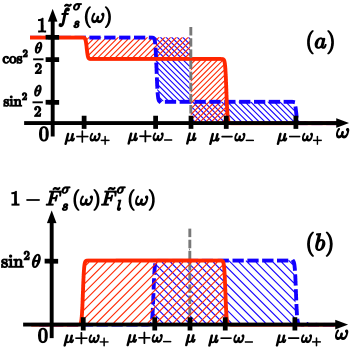
Figure 3: (a) The spin-diagonal part of the small ferromagnet’s rotating-frame distribution function is shown for spin-up (red solid) and spin-down (blue dashed). The areas shaded in blue and red are all equal in size: $\sin^{2}\theta\ |\dot{\phi}|/4$, which means that the electrons are redistributed in energy space for each spin-polarization separately. (b) The noise of charge current, Eq. (11), is determined by the integral over $1-\tilde{F}_{s}^{\sigma}(\omega)\tilde{F}_{l}^{\sigma}(\omega)$, which itself is governed by the distribution function $\tilde{f}_{s}^{\sigma}(\omega)$. The contribution to this noise is identical for both spin-polarizations, as the shaded areas are equal in size (red for spin-up; blue for spin-down). Parameters in figures: $\theta=\pi/3$ and $\omega_{d}<0$.

Adiabatic approximation.—In order to proceed, we have to determine the rotating-frame Green’s function $\tilde{G}_{\lambda}$ for vanishing counting field $\lambda=0$. In principle this poses a complicated problem, since the spin-off-diagonal elements of its inverse $\tilde{G}_{0}^{-1}$ depend on time. However, we assume the magnetization $M$ to be the largest relevant energy scale in the small ferromagnet. This allows us to disregard the spin-off-diagonal elements of $\tilde{G}_{0}^{-1}$ for the determination of $\tilde{G}_{0}$ In particular, we disregard spin-off-diagonal elements of $iR^{\dagger}\dot{R}$ which are related to transitions between spin-up and spin-down states; this corresponds to an adiabatic approximation Shnirman et al. (2015). Furthermore, we disregard spin-off-diagonal elements of the rotated self-energy. It is, now, straightforward to obtain the rotating-frame Green’s function,

$$\begin{split}\tilde{G}_{0,a\sigma}^{R/A}(\omega)&=\frac{1}{\omega-\xi_{a\sigma}\pm i\Gamma_{\Sigma}}\ ,\\ \tilde{G}_{0,a\sigma}^{K}(\omega)&=\frac{-2i\Gamma_{\Sigma}\tilde{F}_{s}^{\sigma}(\omega)}{(\omega-\xi_{a\sigma})^{2}+\Gamma_{\Sigma}^{2}}\ ,\end{split}$$ (8)

with the total level broadening $\Gamma_{\Sigma}=\Gamma_{l}+\Gamma_{r}$. The spin-dependent single-particle energy is $\xi_{a\sigma}=\epsilon_{a}-M\sigma/2$, where $\epsilon_{a}$ are the eigenenergies of $h_{0}$ with corresponding eigenstates $a$. The rotating-frame distribution function of the small ferromagnet,

$$\tilde{F}_{s}^{\sigma}(\omega)=\big{[}\Gamma_{l}\tilde{F}_{l}^{\sigma}(\omega)+\Gamma_{r}\tilde{F}_{r}^{\sigma}(\omega)\big{]}/\Gamma_{\Sigma}\ ,$$ (9)

is a superposition of the leads’ rotating-frame distribution functions. In absence of bias, the rotating-frame distribution functions are exactly the same in all three systems $\tilde{F}_{s}^{\sigma}(\omega)=\tilde{F}_{l}^{\sigma}(\omega)=\tilde{F}_{r}^{\sigma}(\omega)$; see Fig. 3.

It is worthwhile to emphasize that the transformation into the rotating frame is a crucial step that allows us to solve the problem. The reason is as follows. As we discussed above it is enough to find the spin-diagonal components of the rotating-frame distribution function. However, as one can check SM , the knowledge of the spin-diagonal components of the rotating-frame distribution function is not enough in order to determine the distribution function in the laboratory frame.

Charge current and its noise.—The zero-frequency charge current $I_{l}$ is defined via the transported charge $\langle Q_{l}\rangle=\int dt\,I_{l}$. Differentiating the generating function, the transported charge is determined to $\langle Q_{l}\rangle=-i\,\mathrm{tr}[\tilde{G}_{0}\tilde{\Sigma}_{l}^{\prime}]$, where $\tilde{\Sigma}_{l}^{\prime}=\partial_{\lambda}\tilde{\Sigma}_{l}(\lambda)|_{\lambda=0}$ is the derivative of the rotated self-energy $\tilde{\Sigma}(\lambda)=R^{\dagger}\Sigma(\lambda)R$. For the current, we find SM

$$I_{l}=\ \sum_{\sigma}\rho_{\sigma}\Gamma_{l}\int d\omega\,[\tilde{F}^{\sigma}_{l}(\omega)-\tilde{F}_{s}^{\sigma}(\omega)]\ =0\ ,$$ (10)

where we defined the spin-dependent density of states, $\rho_{\sigma}(\omega)=\sum_{a}\frac{1}{\pi}\frac{\Gamma_{\Sigma}}{(\omega-\xi_{a\sigma})^{2}+\Gamma_{\Sigma}^{2}}$. We assumed it to be approximately constant $\rho_{\sigma}(\omega)=\rho_{\sigma}$ on all scales smaller than $M$. The resulting formula for the charge current is the Landauer formula Landauer (1957) with rotating-frame distribution functions. This reflects the fact that the amount of transported charge is an observable which has to be independent of the frame of reference. Explicitly, however, the current vanishes, since no bias is applied.

Similar to the average current, the zero-frequency noise of charge current $S_{l}$ is defined via $\langle\langle Q_{l}^{2}\rangle\rangle=\int dt\,S_{l}/2$. Differentiating the generating function, the noise of transported charge is determined to $\langle\langle Q_{l}^{2}\rangle\rangle=\mathrm{tr}[\tilde{G}_{0}\tilde{\Sigma}_{l}^{\prime\prime}]+\mathrm{tr}[\tilde{G}_{0}^{\prime}\tilde{\Sigma}_{l}^{\prime}]$, where $\tilde{\Sigma}_{l}^{\prime\prime}=\partial^{2}_{\lambda}\tilde{\Sigma}_{l}(\lambda)|_{\lambda=0}$ is the second derivative of the rotated self-energy and $\tilde{G}_{0}^{\prime}=\partial_{\lambda}\tilde{G}_{\lambda}\big{|}_{\lambda=0}=\tilde{G}_{0}\tilde{\Sigma}_{l}^{\prime}\tilde{G}_{0}$ is the derivative of the rotating-frame Green’s function. For the noise, we find SM

$$S_{l} =\sum_{\sigma}g_{\sigma}\int d\omega\,\Big{\{}\big{[}1-\tilde{F}_{s}^{\sigma}(\omega)\tilde{F}_{l}^{\sigma}(\omega)\big{]}+$$

$$\hskip 70.0001pt+\frac{\Gamma_{l}}{\Gamma_{r}}\tilde{F}_{s}^{\sigma}(\omega)\big{[}\tilde{F}_{l}^{\sigma}(\omega)-\tilde{F}_{s}^{\sigma}(\omega)\big{]}\Big{\}}\ ,$$ (11)

where $g_{\sigma}=2\rho_{\sigma}\Gamma_{l}\Gamma_{r}/(\Gamma_{l}+\Gamma_{r})$ is the spin-dependent conductance of the double tunnel-junction. After the integration over frequency, we obtain Eq. (1) as result for the shot noise.

Discussion.— In our relatively simple model which excludes internal relaxation, we were able to properly derive the non-equilibrium distribution function $\tilde{F}_{s}^{\sigma}(\omega)$ given by Eq. (9). This, in particular, guarantees that the charge conservation laws are satisfied. Indeed, since the small ferromagnet cannot store additional charges for an infinite time, charge conservation requires $I_{l}=-I_{r}=:I$ and $S_{l}=S_{r}=:S$ at zero frequency. For the right junction, current $I_{r}$ and noise $S_{r}$ can be obtained from eqs. (10) and (11) by exchanging $\Gamma_{l}\leftrightarrow\Gamma_{r}$ and substituting $\tilde{F}_{l}^{\sigma}(\omega)\rightarrow\tilde{F}_{r}^{\sigma}(\omega)$. As expected, we find $I_{l}=-I_{r}$ and $S_{l}=S_{r}$.

In the presence of internal relaxation one might be tempted to impose a physically motivated distribution function in the small ferromagnet as a shortcut of a full calculation. We emphasize, however, that the charge conservation condition $S_{l}=S_{r}$ puts a strong restriction onto possible distribution functions. In particular, charge conservation would be violated if $\tilde{F}_{s}^{\sigma}(\omega)$ is just replaced by an equilibrium distribution function with an adjusted electrochemical potential. Thus, a straightforward application of the results of Ref. Virtanen and Heikkilä (2017) obtained for a single tunnel junction to the double tunnel-junction considered here is not possible.

We expect the effects of internal relaxation to be threefold: (i) the Gilbert-damping coefficient $\alpha$ can be increased (spin-orbit coupling) and, thereby, the polar angle $\theta$ of steady state precessions is changed; (ii) internal relaxation tends to bring the magnet’s rotating-frame distribution function $\tilde{F}_{s}^{\sigma}(\omega)$ towards equilibrium; (iii) the formal result for the noise, Eq. (11), has to be changed in order not to violate charge conservation when the distribution function changes. However, for weak internal relaxation, these effects might be taken into account perturbatively and, therefore, we expect our results to be robust against finite but small internal relaxation.

Conclusion.— We have found a higher order non-equilibrium off-diagonal response effect. Namely, we have shown that zero-frequency shot noise of charge current is generated by a precessing magnetization of a small ferromagnet which is tunnel-coupled to two normal metal leads. This noise, Eq. (11), crucially depends on the electronic distribution function which is in turn geometrically governed by the magnetization dynamics; see Fig. 3. Thus, the noise of the charge current, Eq. (1), is generated by the precession of the magnetization. For the FMR-setup, Fig. 2, this effect can be used to detect the magnetization dynamics in spite of the vanishing average current.

Acknowledgements.—We thank G. E. W. Bauer, M. Keßler, and W. Wulfhekel for fruitful discussions. This work was supported by DFG Research Grant No. SH 81/3-1. The research of T.L. is partially supported by the Russian Foundation for Basic Research under the Grant No. 19-32-50005. Furthermore, T.L. acknowledges KHYS of KIT and the Feinberg Graduate school of WIS for supporting a stay at WIS; I.S.B. acknowledges RAS Program Topical problems in low temperature physics, the Alexander von Humboldt Foundation, and the Basic research program of HSE; Y.G. acknowledges the DFG Research Grant RO 2247/11-1 and the Italia-Israel QUANTRA.

See pages 1 of Supplement-for-arxiv.pdf See pages 2 of Supplement-for-arxiv.pdf See pages 3 of Supplement-for-arxiv.pdf See pages 4 of Supplement-for-arxiv.pdf

References

- Slonczewski (1996) J. C. Slonczewski, Journal of Magnetism and Magnetic Materials 159, L1 (1996).
- Berger (1996) L. Berger, Phys. Rev. B 54, 9353 (1996), URL https://link.aps.org/doi/10.1103/PhysRevB.54.9353.
- Berger (1999) L. Berger, Phys. Rev. B 59, 11465 (1999), URL https://link.aps.org/doi/10.1103/PhysRevB.59.11465.
- Tserkovnyak et al. (2002) Y. Tserkovnyak, A. Brataas, and G. E. W. Bauer, Phys. Rev. Lett. 88, 117601 (2002), URL https://link.aps.org/doi/10.1103/PhysRevLett.88.117601.
- Brataas et al. (2002) A. Brataas, Y. Tserkovnyak, G. E. W. Bauer, and B. I. Halperin, Phys. Rev. B 66, 060404 (2002), URL https://link.aps.org/doi/10.1103/PhysRevB.66.060404.
- Tserkovnyak et al. (2005) Y. Tserkovnyak, A. Brataas, G. E. W. Bauer, and B. I. Halperin, Rev. Mod. Phys. 77, 1375 (2005), URL https://link.aps.org/doi/10.1103/RevModPhys.77.1375.
- Tserkovnyak et al. (2008) Y. Tserkovnyak, T. Moriyama, and J. Q. Xiao, Phys. Rev. B 78, 020401 (2008), URL https://link.aps.org/doi/10.1103/PhysRevB.78.020401.
- Jonson et al. (2019) M. Jonson, R. Shekhter, O. Entin-Wohlman, A. Aharony, H. Park, and D. Radić, arXiv preprint arXiv:1903.03321 (2019).
- Landauer (1998) R. Landauer, Nature 392, 658 (1998).
- Blanter and Büttiker (2000) Y. M. Blanter and M. Büttiker, Physics reports 336, 1 (2000).
- Foros et al. (2009) J. Foros, A. Brataas, G. E. W. Bauer, and Y. Tserkovnyak, Phys. Rev. B 79, 214407 (2009), URL https://link.aps.org/doi/10.1103/PhysRevB.79.214407.
- Arakawa et al. (2015) T. Arakawa, J. Shiogai, M. Ciorga, M. Utz, D. Schuh, M. Kohda, J. Nitta, D. Bougeard, D. Weiss, T. Ono, et al., Phys. Rev. Lett. 114, 016601 (2015), URL https://link.aps.org/doi/10.1103/PhysRevLett.114.016601.
- Kamra and Belzig (2016a) A. Kamra and W. Belzig, Phys. Rev. B 94, 014419 (2016a), URL https://link.aps.org/doi/10.1103/PhysRevB.94.014419.
- Kamra and Belzig (2016b) A. Kamra and W. Belzig, Phys. Rev. Lett. 116, 146601 (2016b), URL https://link.aps.org/doi/10.1103/PhysRevLett.116.146601.
- Cascales et al. (2015) J. P. Cascales, D. Herranz, U. Ebels, J. A. Katine, and F. G. Aliev, Applied Physics Letters 107, 052401 (2015).
- Virtanen and Heikkilä (2017) P. Virtanen and T. T. Heikkilä, Phys. Rev. Lett. 118, 237701 (2017), URL https://link.aps.org/doi/10.1103/PhysRevLett.118.237701.
- Horovitz and Golub (2019) B. Horovitz and A. Golub, arxiv [cond-mat] p. 1904.11221v1 (2019).
- Ludwig et al. (2017) T. Ludwig, I. S. Burmistrov, Y. Gefen, and A. Shnirman, Phys. Rev. B 95, 075425 (2017), URL https://link.aps.org/doi/10.1103/PhysRevB.95.075425.
- Ludwig et al. (2019) T. Ludwig, I. S. Burmistrov, Y. Gefen, and A. Shnirman, Phys. Rev. B 99, 045429 (2019), URL https://link.aps.org/doi/10.1103/PhysRevB.99.045429.
- Kamenev (2011) A. Kamenev, Field Theory of Non-Equilibrium Systems (Cambridge University Press, 2011).
- Kamenev and Levchenko (2009) A. Kamenev and A. Levchenko, Advances in Physics 58, 197 (2009), eprint https://doi.org/10.1080/00018730902850504, URL https://doi.org/10.1080/00018730902850504.
- Altland and Simons (2010) A. Altland and B. D. Simons, Condensed matter field theory (Cambridge University Press, 2010).
- Shnirman et al. (2015) A. Shnirman, Y. Gefen, A. Saha, I. S. Burmistrov, M. N. Kiselev, and A. Altland, Phys. Rev. Lett. 114, 176806 (2015), URL https://link.aps.org/doi/10.1103/PhysRevLett.114.176806.
- (24) See Supplemental Material.
- Landauer (1957) R. Landauer, IBM Journal of Research and Development 1, 223 (1957).