Learning Transient Universe in Near-Ultraviolet By Wide-angle Cameras

Abstract

We perform a detailed analysis and simulations on the transient detection capability in the near-ultraviolet (NUV) band by focusing on some major local transient events. These events include the tidal disruption event due to a supermassive blackhole, the shock breakout of a core-collapse supernova and the flare of a late-type star. Our simulations show that a set of small wide-angle NUV cameras can allow us to detect and study numerous galactic and extra-galactic transient events. Based on the analysis and simulations, here we propose a space-based NUV sky patrol mission by updating the proposal that was originally submitted to the Chinese Space Station mission in 2011. The mission proposed here is composed of a set of eight small wide-field NUV cameras each with a diameter of 20cm. The total sky area simultaneously covered by the NUV cameras is as large as 3000$\mathrm{deg^{2}}$. The survey cadence ranges from 30 to 300s. The transient events are required to be detected by a dedicated on-board software in real time.

1 Introduction

Time-domain astronomy, which mainly explores the Universe by searching for and studying transients in different wavelength bands, is a hot topic of modern astronomy. Transient phenomena have been widely explored in high energy bands (i.e., X-ray and $\gamma$-ray) in the past decades, thanks to the great success achieved by the Neil Gehrels Swift Observatory (Gehrels et al. 2004) and the Fermi Gamma-ray Space Telescope (e.g., Atwood et al. 2009; Meegan et al. 2009). This success enables us to make great progress in the understanding of Gamma-ray bursts (GRBs, see a review in Woosley & Bloom 2006). The capability of exploring transients in X-ray and $\gamma$-ray will be continued by forthcoming missions, including SVOM (Wei et al. 2016) and the Einstein Probe (EP) (Yuan et al. 2015).

In addition to the high energy bands, transient phenomena have been comprehensively probed by a lot of optical time-domain surveys in recent years, because of the great progress made in both detector and computation technology in the past decades. Some ongoing optical survey programs include: the Pan-STARRS1 survey (PS1; Chambers et al. 2016), the Asteroids Terrestrial-impact Last Alert System (ATLAS; Tonry et al. 2018), the Palomar Transient Factory (PTF; Law et al. 2009) and the successor Zwicky Transient Facility (ZTF; Kulkarni 2018), the All-Sky Automated Survey for Supernovae (ASAS-SN; Shappee et al. 2014), Pi of the sky (Burd et al. 2005), RAPTOR (Vestrand et al. 2002), and the Ground Wide-Angle Cameras system (GWAC, Wei et al. 2016). These optical transient surveys discovered an abundance of supernovae (SNe) in diverse types and the related phenomena (e.g., Gal-Yam et al. 2014; Arcavi et al. 2017; Whitesides et al. 2017), a number of tidal disruption events (TDEs) induced by supermassive blackholes (SMBHs, e.g., Holoien et al. 2018 and reference therein), “Changing-look” active galactic nuclei (CL-AGNs, e.g., Gezari et al. 2017; Wang et al. 2018), and some mysterious fast-evolving luminous transients without a convincing explanation (e.g., Rest et al. 2018 and references therein). The forthcoming Large Synoptic Survey Telescope (LSST) project (LSST Science Collaboration et al. 2017) will be a milestone for optical transient survey. The transient sky has been monitored by LOFAR (e.g., Gunst & Bentum 2007; de Vos et al. 2007) and the SKA in radio.

In addition to electromagnetic radiation, a non-electromagnetic message transmitted by a gravitational-wave (e.g., the Advanced LIGO, Harry 2010; Aasi et al. 2015; LIGO Scientific Collaboration et al., 2015, the Advanced Virgo, Acernese et al. 2009; Accadia et al. 2012; Acernese et al. 2015; KAGRA, Somiya 2012; Aso et al. 2013) and by neutrino events (e.g., the IceCube experiment, Aartsen et al. 2015) has been used to explore transient phenomena. Operation of Advanced LIGO opened an era of multi-message astronomy by successfully detecting the gravitational-wave signals emitted from the coalescence of a binary black holes (BBHs, e.g., GW 150914, Abbott et al. 2016) and the coalescence of a binary neutron stars (BNS, GW 170817. e.g., Abbott et al. 2017). The coalescence of binary neutron stars was confirmed by the detection of electromagnetic emission from the associated kilonova (e.g., Shappee et al. 2017; Drout et al. 2017; Evans et al. 2017).

Time-domain astronomy is, however, rarely developed in ultraviolet (UV) bands, even though the study of transients in UV can potentially address some major scientific questions (e.g., Sagiv et al. 2014; Brosch et al. 2014). In fact, observations carried out by Swift/UVOT and GALEX (Martin et al. 2005) returned exciting results on transients (e.g., Soderberg et al. 2008; Schawinski et al. 2008), although both instruments are not designed to search for transients based on a large field-of-view (FoV). The main scientific goal of GALEX is to study star formation and galaxy evolution in UV bands, which results in very limited time-domain observations.

In the development of the Chinese Space Station mission, we proposed a wide-angle time domain survey in near-UV (NUV) as early as in 2011. Subsequent studies, however, indicated that the Space Station is not an ideal platform for this survey. The depth of the survey is limited because the on-board cameras can only work in drift scan mode.

In this paper, we perform a detailed analysis on the detection capability of an NUV wide-angle time domain survey. The analysis focuses on some important scientific objects. One can see from our analysis that an abundance of results can be obtained by a set of small NUV cameras. Based on this analysis, we then propose a small satellite mission dedicated to the NUV wide-angle time domain survey.

The paper is organized as follows. Section 2 describes the major scientific motivations for the proposed NUV transient survey by supplementing the CL-AGN phenomenon. The analysis and simulation of detection capability are presented in Section 3. Section 4 describes the concept of the proposed dedicated NUV transient survey mission. A $\Lambda$CDM cosmology with parameters $H_{0}=70\mathrm{km\ s^{-1}\ Mpc^{-1}}$, $\Omega_{m}=0.3$, and $\Omega_{\Lambda}=0.7$ is adopted throughout the paper

2 Scientific Objectives

For transient phenomena that can be preferably explored in the UV band, we refer readers to the excellent review given by Sagiv et al. (2014, and references therein). The phenomena described in that review include: the supernova shock breakout (SBO) resulting from the explosive death of a massive star; the TDE of a main-sequence star (or a white dwarf) due to the tidal force of a supermassive (or intermediate massive) blackhole; the variability of AGNs; and the flare of stars.

Besides the topics described in the review, here we pay more attention to the CL-AGN phenomenon from a scientific perspective, because the phenomenon is a hot and challenging topic in modern astronomy. According to their observed optical spectra, AGNs can be classified into Type-1 and Type-2 AGNs. The spectra of Type-1 AGNs have both broad ($\mathrm{FWHM>1000\ km\ s^{-1}}$) and narrow ($\mathrm{FWHM\sim 10^{2}\ km\ s^{-1}}$) Balmer emission lines. On the contrary, only narrow Balmer emission lines can be identified in Type-2 AGNs. The two types can be unified by the widely accepted unified model based on the orientation effect caused by the dust torus (see Antonucci 1993 for a review). This successful model has, however, been recently challenged by the discovery of so-called CL-AGNs that show a change in their spectral types on a time scale of several years.

Although both “turn-on” and “turn-off” type transitions have been revealed in past years, there are only 40 identified CL-AGNs at present (e.g., Shapovalova et al. 2010; Shappee et al. 2014; LaMassa et al. 2015; McElroy et al. 2016; Runnoe et al. 2016; Gezari et al. 2017; Yang et al. 2018; Ruan et al. 2016; MacLeod et al. 2016; Wang et al. 2018). The discovery of CL-AGNs is actually a hard and expensive task, which requires repeated spectroscopy to identify a change in the spectral type of the Balmer line profiles. At the same time, an optical transient survey is not a good way to select CL-AGN candidates because of the serious contamination caused by AGN’s normal variation in optical bands.

The origin of CL-AGNs is still under debate, even though there is accumulating evidence supporting the fact that it is likely due to a variation in SMBH accretion rate that results from either a viscous radial inflow or disk instability (e.g., Yang et al. 2018; Wang et al. 2018; Gezari et al. 2017). In addition, other explanations include: (1) a variation in the obscuration if the torus has a patchy configuration (e.g., Elitzur 2012); (2) an accelerating outflow launched from the central SMBH (e.g., Shapovalova et al. 2010); and (3) a TDE (e.g., Merloni et al. 2015; Blanchard et al. 2017).

Besides the prominent line profile change, CL-AGNs are typically accompanied by a significant variation in their blue featureless continuum, because Type-1 and Type-2 AGNs differ significantly in their UV continuum. This significant difference in continuum means an NUV transient survey is the best way to find both “turn-on” and “turn-off” CL-AGNs in the local Universe.

3 Detection Rate Predictions

For a wide-angle time domain survey in NUV, the detection rates of some important scientific objects are predicted in this section.

3.1 UV Brightness Estimated from X-ray Flux

At the beginning, we estimate the NUV brightness of some transients from their soft X-ray flux. A powerlaw photon spectrum of $N(E)=N_{0}E^{-\Gamma}$ is adopted for GRBs, SBOs, and TDEs. The corresponding X-ray flux $f_{\mathrm{X}}$ within the energy range from $E_{1}$ to $E_{2}$ can be written as an integral of $f_{\mathrm{X}}=\int_{E_{1}}^{E_{2}}N(E)EdE=N_{0}\int_{E_{1}}^{E_{2}}E^{1-\Gamma}dE$, which allows us to obtain the specific flux $f_{\nu}$ at a given wavelength $\lambda$ as

$$f_{\nu}=EN(E)\frac{dE}{d\nu}=\frac{\lambda f_{\mathrm{X}}}{c}\bigg{[}\frac{2-\Gamma}{(E_{2}/E)^{2-\Gamma}-(E_{1}/E)^{2-\Gamma}}\bigg{]}$$ (1)

when $\Gamma\neq 2$, and

$$f_{\nu}=EN(E)\frac{dE}{d\nu}=\frac{\lambda f_{\mathrm{X}}}{c}\ln^{-1}\bigg{(}\frac{E_{2}}{E_{1}}\bigg{)}$$ (2)

when $\Gamma=2$. Based on the traditionally used Band function (Band et al. 1993), the values of $\Gamma$ are adopted to be 1.0 and 0.5 for Long GRBs and short GRBs, according to the BASTE and Fermi observations (e.g., Abdo et al. 2009; Zhang et al. 2011, Nova et al. 2011). A soft spectrum with a $\Gamma=2.0$ is used for SBOs and TDEs. In fact, the XMM-Newton spectrum of TDE RXJ1242 C1119 has an index of $\Gamma=2.5$, although the initial spectrum taken by ROSAT has an index of $\Gamma\simeq 5$ (e.g., Komossa 2017; Komossa et al. 2004; Halpern et al. 2004). In fact, similar spectral hardening has been observed in a few TDEs (e.g., Komossa & Bade 1999; Nikolajuk & Walter 2013). Soderberg et al. (2008) revealed a X-ray spectrum with a photon index of $\Gamma=2.3\pm 0.3$ in SBO event of SN 2008D.

We estimate the UV brightness of a stellar flare from its soft X-ray flux according to the Neupert effect which suggests a correlation between soft X-ray luminosity and UV energy release (e.g., Gudel et al. 2002; Hawley et al. 1995). A average ratio of X-ray to NUV specific luminosity of 20 is adopted in our estimation.

The corresponding magnitude in the AB system is then determined from the definition (Fukugita et al. 1996)

$$\mathrm{mag_{AB}}=-2.5\log f_{\nu}-48.6+A_{\lambda}$$ (3)

where $A_{\lambda}$ denotes the extinction at wavelength $\lambda$. Table 1 lists the calculated magnitudes at different X-ray flux levels, in which $\lambda=2800$Å, $A_{\lambda}(2800\AA)=0.2$mag, $E_{1}=0.5$keV and $E_{2}=4.0$keV are adopted. The $A_{\lambda}(2800\AA)$ is estimated from the $V$-band extinction through the extinction curve of LMC provided in Gordon et al. (2003), by assuming $A_{V}=0.1$mag.

Table 1: UV brightness estimated from different soft X-ray fluxes.

$f_{x}$	$\mathrm{mag_{AB}}$	$\Gamma$	Transients
$\mathrm{erg\ s^{-1}\ cm^{-2}}$		mag
(1)	(2)	(3)	(4)
$10^{-7}$	14.3	1.0	LGRB
$10^{-8}$	17.7	1.0	LLGRB
	20.0	0.5	SGRB
$10^{-9}$	19.3	1.0	LLGRB
	12.6	2.0	SBO
$10^{-10}$	15.1	2.0	SBO, TDE
	9.8		stellar flare
$10^{-11}$	17.6	2.0	SBO,TDE
	12.3		stellar flare

3.2 Comparison of Spectral Energy Distributions

Compared to surveys in optical, one of the advantages of an NUV time-domain survey is the extremely low brightness of the host galaxies of extra-galactic transients. To clarify this fact, here we compare the SEDs of TDEs and of SBOs to those of their hosts. It is emphasized that the host galaxies are hard to spatially resolve in a wide-angle survey, except for very nearby galaxies.

3.2.1 TDEs

For a given SMBH with a mass of $M_{\mathrm{BH}}$, the SED of a TDE of a main-sequence star with mass $M_{*}$ is modeled by following Lodato & Rossi (2011) by including the contributions from both a hot accretion disk and a disk wind.

When the effect due to the disk wind is considered, the disk temperature $T_{d}$ can be written as a function of the distance $R$ from the central SMBH as (Strubbe & Quataert 2009)

$$\sigma T_{d}^{4}=\frac{3GM_{\mathrm{BH}}\dot{M}f}{8\pi R^{3}}\bigg{\{}\frac{1}{2}+\bigg{[}\frac{1}{4}+\frac{3}{2}f\bigg{(}\frac{\dot{M}}{\eta\dot{M}_{\mathrm{Edd}}}\bigg{)}^{2}\bigg{(}\frac{R_{\mathrm{S}}}{R}\bigg{)}^{2}\bigg{]}^{1/2}\bigg{\}}^{-1}$$ (4)

where $R_{\mathrm{S}}=2GM_{\mathrm{BH}}/c^{2}$ is the Schwartzchild radius of the SMBH, $\dot{M}_{\mathrm{Edd}}=1.3\times 10^{18}(M_{\mathrm{BH}}/M_{\odot})(\eta/0.1)^{-1}\ \mathrm{g\ s^{-1}}$ is the Eddington accretion rate, and $f=1-\sqrt{R_{\mathrm{in}}/R}$. We adopt the innermost stable circular orbit of the disk $R_{\mathrm{in}}=3R_{\mathrm{S}}$ throughout the subsequent analysis. The accretion rate $\dot{M}$ is related to the fallback rate $\dot{M}_{\mathrm{fb}}$ as $\dot{M}=(1-f_{\mathrm{out}})\dot{M}_{\mathrm{fb}}$. The factor $f_{\mathrm{out}}$ accounts for the outflow effect due to the disk wind, which can be expressed as (Ditan & Shviv 2010)

$$f_{\mathrm{out}}=\frac{2}{\pi}\arctan\bigg{[}\frac{1}{7.5}\bigg{(}\frac{\dot{M}_{\mathrm{fb}}}{\dot{M}_{\mathrm{Edd}}}-1\bigg{)}\bigg{]}$$ (5)

for super Eddington accretion. $\dot{M}_{\mathrm{fb}}\propto t^{-5/3}$, which has a peak value of

$$\dot{M}_{\mathrm{fb,p}}=1.9\times 10^{26}M_{\mathrm{BH,6}}^{-1/2}m_{*}^{2}\beta^{3}x_{*}^{-3/2}\mathrm{g\ s^{-1}}$$ (6)

where $M_{\mathrm{BH,6}}=M_{\mathrm{BH,}}/10^{6}M_{\odot}$, $m_{*}=M_{*}/M_{\odot}$, $x_{*}=R_{*}/R_{\odot}$, and $\beta=r_{t}/r_{p}$. $r_{t}=10^{-2}M_{\mathrm{BH,6}}^{1/3}m_{*}^{-1/3}x_{*}R_{\odot}$ is the tidal disruption radius and $r_{p}$ the periastron radius.

Because the emission from the hot accretion disk is dominant in soft X-ray and UV, the photosphere model was proposed to explain the optical emission detected in some TDEs (e.g., Guillochon et al. 2014; Roth et al. 2015; Jiang et al. 2016; Metzger & Stone 2016). Based on basic energy conservation, the radius and temperature of the photosphere at the peak time are (Lodato & Rossi 2011)

$$r_{\mathrm{ph}}\approx 1.4\times 10^{15}\bigg{(}\frac{f_{\mathrm{out}}}{f_{\upsilon}}\bigg{)}\beta^{5/2}M_{\mathrm{BH,6}}^{-5/6}x_{*}^{-1}m_{*}^{11/6}\ \mathrm{cm}$$ (7)

$$T_{\mathrm{ph}}\approx 1.6\times 10^{4}\bigg{(}\frac{f_{\mathrm{out}}}{f_{\upsilon}}\bigg{)}^{-1/12}\beta^{-23/24}M_{\mathrm{BH,6}}^{-41/73}x_{*}^{1/3}m_{*}^{-53/72}\ \mathrm{K}$$ (8)

where $f_{\upsilon}\geq 1$, in the unit of escape velocity, is a parameter describing the wind velocity.

The total emission is therefore the combination of two components

$$L_{\nu}=4\pi^{2}\int_{R_{\mathrm{in}}}^{R_{\mathrm{out}}}RB_{\nu}(T_{d})dR+4\pi^{2}r_{\mathrm{ph}}^{2}B_{\nu}(T_{\mathrm{ph}})$$ (9)

where $B_{\nu}(T)$ is the Planck function and $R_{\mathrm{out}}\approx 15\beta^{-1}M_{6}^{-1/2}m_{*}^{-1/3}x_{*}R_{\mathrm{in}}$ is the outer distance of the disk .

Figure 1 compares the predicted UV-to-optical SEDs of the TDEs to the modeled SEDs of the corresponding host galaxies. The four panels correspond to four cases with different $M_{\mathrm{BH}}$. The following fiducial values are adopted in the predictions: $m_{*}=x_{*}=\beta=1$, $\eta=0.1$, and $f_{\upsilon}=1$. An UV-to-optical spectrum with an age of 1.4Gyr and a metalicity of 0.05$Z_{\odot}$ is first extracted from the single stellar population (SSP) spectral library built by Bruzual & Charlot (2003). The luminosity level of the spectrum is then scaled to the bulge of the corresponding host galaxy through the firmly established $M_{\mathrm{BH}}-L_{\mathrm{bulge}}$ relationship: $\log M_{\mathrm{BH}}=9.23+1.11\log(L_{\mathrm{bulge}}/10^{11}L_{\odot})$ (McConnell & Ma 2013). Two facts can be learned from the comparison shown in the Figure 1. On the one hand, the TDEs are brighter than their host galaxies by 1-3 orders of magnitudes in the FUV band in all the four cases. The NUV band is quite sensitive to the TDEs with a blackhole mass of $10^{6}M_{\odot}$ by a brightness excess of about 3 orders of magnitudes, and is also plausible for a case with a blackhole mass either $\sim 10^{5}M_{\odot}$ or $\sim 10^{7}M_{\odot}$. On the other hand, it is a hard task to detect a TDE in optical bands in the case with an SMBH more massive than $10^{6}M_{\odot}$.

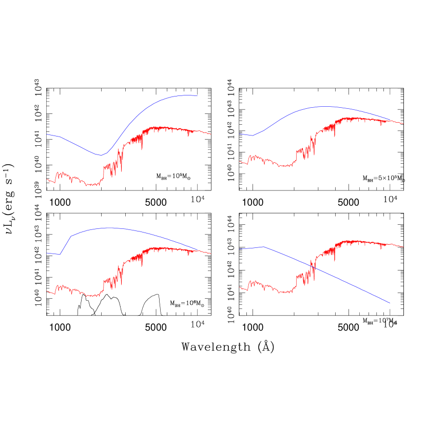
Figure 1: In each panel, the predicted TDE’s SED (the blue curve) is compared to the modeled SED of the corresponding bulge (the red curve). Different panels correspond to different SMBH mass. The transmission curves of the FUV, NUV, and SDSS $g$ band are shown in the left-bottom panel by black curves.

Table 2: The parameters used for detection rate estimations.

Item	Value
(1)	(2)
$d$	20cm
$\eta$	0.3
RN	$4e^{-}$
CCD pixels	4k$\times$4k
$n_{\mathrm{pix}}$	9 pixels
$\lambda_{0}$	2000Å
$\Delta\lambda$	500Å
Exposure time	TDEs: 3000s, SBOs: 300s and flares: 30s
$\mathrm{S/N}$ threshold	7

3.2.2 SBO

The spectrum of both an SBO and the following shock cooling can be described well as a blackbody with a temperature of $10^{4-5}$K (e.g., Matzner & McKee 1999; Sapir & Halbertal 2014). Figure 2 compares the spectrum of a blackbody at a temperature of $1\times 10^{5}$K to those of the galaxies with different total masses ranging from $10^{9}$ to $10^{11}M_{\odot}$. The specific luminosity of the blackbody spectrum is determined by requiring its NUV flux to equal the observed flux of Type II-P SN SNLS-04D3dc (Schawinski et al. 2008; Gezari et al. 2008) at $z=0.1854$, i.e., $f_{\nu}=5\times 10^{-29}\ \mathrm{erg\ s^{-1}\ cm^{-2}\ Hz^{-1}}$. The host galaxy spectra used for comparison have an age of 1.4Gyr, which are extracted from the SSP spectra library again. The total light of the galaxies is involved in the comparison by taking into account the poor spatial resolution of a wide-angle survey. Similar to the case of TDE, the comparison shows that NUV the time-domain survey is more powerful for detecting SBOs than optical surveys.

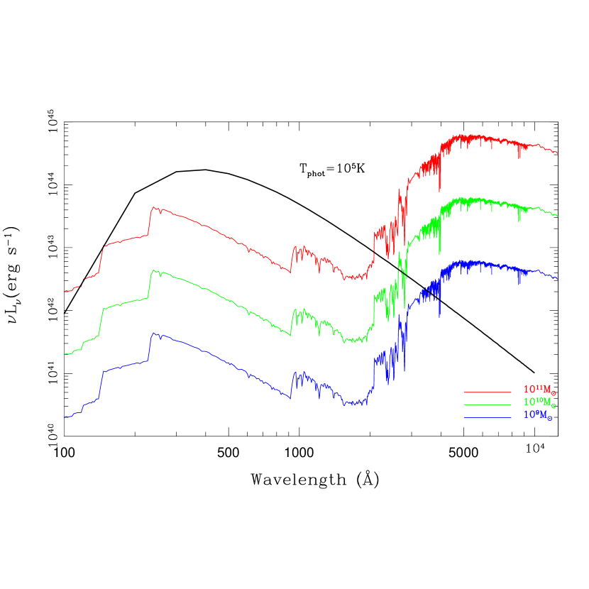
Figure 2: The SED (the black curve) of an SBO with a temperature of $10^{5}$k is compared to the SED of the total light of host galaxies with different total masses.

3.3 Detection Rates

After showing that contamination due to the underlying host galaxies is negligible in an NUV survey, we then predict the detection rates for TDEs, SBOs, and superflares of G- and late-type stars, for a wide-angle time-domain survey in NUV. The survey is assumed to be carried out by a set of wide-angle cameras that monitor different sky areas simultaneously. Each camera is assumed to be equipped with a 4k$\times$4k CCD as the detector.

We first determine the limiting magnitude of individual camera from the simplified “CCD” equation (Merline & Howell 1995; Mortara & Fowler 1981; Gullixson, 1992 and cf. NOAO/KPNO CCD instrument manuals)

$$\frac{S}{N}\simeq\frac{\eta N_{*}t}{\sqrt{\eta N_{*}t+n_{\mathrm{pix}}(\eta N_{b}t+RN^{2})}}$$ (10)

where $t$ is the exposure time and $RN$ the readout noise of each pixel. $n_{\mathrm{pix}}$ and $\eta$ are the number of pixels occupied by a single star and the system total efficiency, respectively, which depend on the optical design and detector technology. $N_{*}$ is the photon rate from the source and $N_{b}$ the photon rate per pixel due to sky background.

For an observation carried out in a bandwidth of $\Delta\lambda=\lambda_{2}-\lambda_{1}$, we have

$$N_{*}=\frac{1}{16h}\bigg{(}\frac{d}{d_{L}}\bigg{)}^{2}\int_{\nu_{1}}^{\nu_{2}}L_{\nu}d\ln\nu$$ (11)

for a given source with a specific luminosity $L_{\nu}$ and a luminosity distance of $d_{L}$, and

$$N_{b}=\frac{1}{4}\pi d^{2}\int_{\Delta\Omega_{p}}\int_{\nu_{1}}^{\nu_{2}}R_{\nu}d\nu d\Omega$$ (12)

where $R_{\nu}$ is the sky background photon flux per solid angle at frequency $\nu$ and $\Delta\Omega_{p}$ the solid angle corresponding to each pixel. The parameter $d$ is the diameter of each camera. Based on the experience of GALEX, the sky background brightness is typically 27.5(26.5)$\mathrm{mag\ arcsec^{-2}}$, which corresponds to a photon flux of $1\times 10^{-6}(10^{-5})\ \mathrm{photons\ s^{-1}\ cm^{-2}\ arcsec^{-2}}$ in the FUV and NUV bands, respectively (Martin et al. 2005). $\Delta\Omega_{p}$ can be determined by $\Delta\Omega_{p}=(\alpha d_{p})^{2}$, where $\alpha=206265\arcsec/f$ and $f$ is the focal length, and $d_{p}$ is the CCD pixel size.

For an observation carried out with both a given exposure time and a fixed pixel scale, the limiting magnitude can be obtained from Eq. (9) for a given signal-to-noise (S/N) ratio threshold. In the limiting magnitude estimation, we only consider the limiting case in which noise is dominated by both the sky background and readout noise. We multiply a factor of 10 to the used background counter rate to take into account of the noise contributed by potential stray light, dark current, and flatfield correction.

3.3.1 TDE

The detection rate of TDEs occurring in the Universe at $z\ll 1$ is estimated by following Strubbe & Quataert (2009)

$$\tiny\Gamma_{\mathrm{TDE}}=\int_{\Delta\Omega}\int_{0}^{z_{\mathrm{max}}}\int_{M_{\mathrm{BH}}}\int_{R_{p}}^{R_{T}}\frac{dn}{d\ln M_{\mathrm{BH}}}\frac{d\gamma}{d\ln R_{p}}\frac{dV}{dzd\Omega}d\ln R_{p}d\ln M_{\mathrm{BH}}dzd\Omega$$ (13)

where $\gamma$ is the tidal distribution rate for a single SMBH. We ignore the dependence of $\gamma$ on $R_{p}$, and adopt the value of $\gamma=10^{-5}\ \mathrm{yr^{-1}}$ reported in Donley et al. (2002), which results in $d\gamma/d\ln R_{p}=\gamma/\ln(R_{T}/R_{p})$. $z_{\mathrm{max}}$ is the maximum redshift that is determined from both the intrinsic luminosity and limiting magnitude calculated above. We adopt a universal SMBH density $n\simeq 10^{-2}\mathrm{Mpc^{-3}}$ predicted in Hopkins et al. (2007), although the density falls slightly at the high mass end. $\Delta\Omega=N\delta\Omega$ is the total sky area that is simultaneously surveyed by a set of $N$ cameras, and each camera has an FoV of $\delta\Omega$.

The lower panel in Figure 3 shows the estimated detection rates $\Gamma_{\mathrm{TDE}}$ in the cases with different $N$, as a function of $\Delta\Omega$. The fiducial parameters used in the predictions are listed in Table 2. One can see from the figure that for a given $\Delta\Omega$, $\Gamma_{\mathrm{TDE}}$ generally increases with $N$, which can be understood by a reduced sky-background noise resulting from a decreasing value of $\Delta\Omega_{p}$. In the case of a given $N$, although $\Gamma_{\mathrm{TDE}}$ generally increases with $\Delta\Omega$, the increment decreases evidently with $\Delta\Omega$. The decreased increment results from an enhanced sky-background noise (i.e., an enhanced $\Delta\Omega_{p}$) that neutralizes the increment caused by an enhancement in total sky coverage.

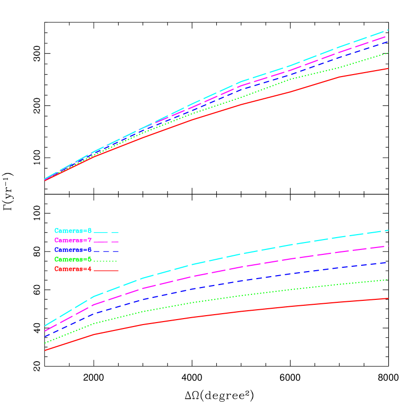
Figure 3: Lower panel: the predicted detection rates for the TDE cases plotted against the total sky area covered by an NUV time-domain survey. The different colors represent the predictions with different numbers of cameras. Upper panel: the same as the lower panel but for the SBO cases.

3.3.2 SBOs

With the $z_{\mathrm{max}}$ determined from the “CCD” equation, we estimate the detection rate of and SBO, $\Gamma_{\mathrm{SBO}}$ through the integral

$$\Gamma_{\mathrm{SBO}}=\int_{\Delta\Omega}\int_{0}^{z_{\mathrm{max}}}f_{\mathrm{SNII}}R_{\mathrm{SN}}\frac{dV}{dzd\Omega}dzd\Omega$$ (14)

where $f_{\mathrm{SNII}}=0.634$ is the fraction of type-II SNe in core-collapse (CC) SNe (Li et al. 2011). $R_{\mathrm{SN}}=k_{\mathrm{cc}}\psi(z)$, in which $k_{\mathrm{cc}}=0.0068M_{\odot}^{-1}$ is the CC-SNe conversion efficiency per stellar mass based on the Salpter initial mass function (IMF) with $m_{\mathrm{min}}=8M_{\odot}$ and $m_{\mathrm{max}}=30M_{\odot}$ (e.g., Walmswell & Eldridge 2012; Tanaska et al. 2016). $\psi(z)$ is the cosmic star formation rate (Madau & Dickison 2014):

$$\psi(z)=0.015\frac{(1+z)^{2.7}}{1+[(1+z)/2.9]^{5.6}}\ \mathrm{M_{\odot}\ yr^{-1}\ Mpc^{-3}}$$ (15)

The predicted detection rates, which are similar to the TDE cases, can be found in the upper panel of Figure 3.

3.3.3 Super Flares of solar-like stars and M dwarfs

Solar-like stars (i.e., type G and K dwarfs) and M dwarfs frequently show super flares with releases of energy of $10^{33-36}$erg and $10^{32-35}$erg, respectively. The energy is mainly radiated from the corona and chromosphere in soft X-ray and UV bands. It makes the flares more easily detected in an NUV time-domain survey since the UV emission of the quiescent counterparts is much weaker than that of the flares. We predict the detection rates of super flares for solar-like stars and M dwarfs by the following estimation

$$\Gamma_{\mathrm{flares}}=\int_{\Delta\Omega}\int_{0}^{r_{E_{1}}}\int_{m_{1}}^{m_{2}}4\pi r^{2}\rho_{\star}\int_{E_{1}}^{E_{2}}\frac{dn}{dm}\frac{dN}{dE}dEdrd\Omega dm$$ (16)

where $dN/dE\propto E^{-\alpha}$ is the flare frequency distribution function that is normalized by an occurrence rate of $2.3\times 10^{-3}\ \mathrm{flares\ yr^{-1}\ star^{-1}}$ (Shibayama et al. 2013), and $dn/dm$ is the normalized Salpeter IMF. Previous statistical studies show that $\alpha\sim 2$ for both G and M dwarfs (e.g., Maehara et al. 2012; Crosby et al. 1993; Aschwanden et al. 2000a,b; Schrijver et al. 2012; Shibayama et al. 2013; Yang et al. 2017). $r_{E_{1}}$, which can be determined through the “CCD” equation, is the maximum distance detectable for a super flare having a released energy of $E_{1}$. In our estimation, the stellar density $\rho_{\star}$ for stars near the Sun is adopted to be 0.14 $\mathrm{star\ pc^{-3}}$ (Gregersen 2010).

Figure 4 shows the predicted detection rates for both type G and M dwarfs as a function of sky area coverage. Compared to the TDE cases, the effect on detection rate caused by the number of cameras is slight since the background noise is reduced significantly due to the short exposure (i.e., 30 seconds).

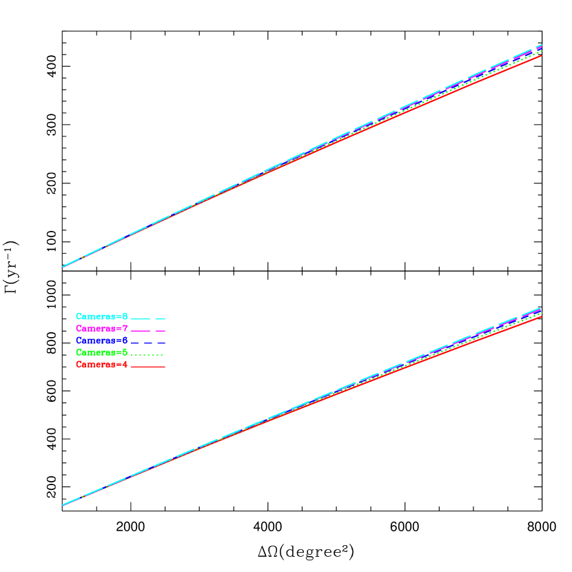
Figure 4: The same as in Figure 3 but for flares occurring in G (the upper panel) and M (the lower panel) dwarfs.

4 Mission Concept

By updating the concept proposed about the Chinese Space Station in 2011, here we propose a small satellite mission dedicated to an NUV wide-angle time domain survey. A dedicated transient survey in the NUV band is still rare. To our knowledge, there are only two proposed missions in the works. One is the ULtraviolet TRansient Astronomical SATellite (ULTRASAT) (Sagiv et al. 2014), and the other is the Wide-field Ultraviolet Imagers available for different platforms (Mathew et al. 2018).

The instruments proposed by us are composed of a set of NUV wide-angle cameras that are used for detecting transient events. With the predictions described in the last section, the NUV wide-angle camera array is proposed to contain eight cameras that provide a total sky coverage of 3000$\mathrm{deg^{2}}$. The FoV and focal length of each camera are $20\times 20\mathrm{deg^{2}}$ and 260mm, respectively. Each of the cameras has a diameter of 20cm. An NUV-enhanced 6k$\times$6k CCD with $\delta$-doping technology (Nikzad et al. 2011) is equipped on each camera at the focal plane. The pixel size of the CCD is 15$\mathrm{\mu m\ pixel^{-1}}$, which yields a spatial resolution of $12\arcsec\ \mathrm{pixel^{-1}}$.

The cadence of the proposed survey ranges from 30s to 300s, which is necessary for detecting star flares and SBOs. Dedicated on-board software will be developed to detect transient events in real time not only from single exposures, but also from combined images. After a transient alert is generated, the alert and corresponding sub-images centered on the transient should be transmitted to the ground. The mission requires not only a suppression of the light pollution resulting from stray light, but also a continuous, unobstructed FoV of the celestial sphere. Both issues could be addressed by a selection of a high Earth orbit. We suggest that the low-cost eccentric “P/2-HEO” orbit (Gangestad et al. 2013) adopted by the Transiting Exoplanet Survey Satellite (TESS) mission (Ricker et al. 2015) is a good solution for both issues. The mission is proposed to adopt an anti-solar pointing law, which enables ground facilities to follow-up the transients in both imaging and spectroscopy as soon as possible.

5 Conclusion

By performing an analysis and simulations on the detection ability in the NUV band for some major transient events (i.e., TDEs, SBOs and flares of stars), here we propose an updated space-based patrol mission dedicated to searching for NUV transient events. The proposed mission stems from the original proposal submitted for the Chinese Space Station mission. The updated mission is composed of a set of eight small wide-field NUV cameras, each with a diameter of 20cm. The total sky area simultaneously covered by the NUV cameras can be as large as 3000deg². The survey cadence is designed to range from 30 to 300s.

References

- Aartsen et al. (2015) Aartsen, M. G., Abraham, K., Ackermann, M., et al. 2015, Phys. Rev. Lett., 115, 081102
- Aasi et al. (2015) Aasi, J. et al. 2015, Class Quantum Grav, 32, 074001
- Abbott et al. (2016) Abbott, B. P., Abbott, R., Abbott, T. D., et al. 2016, ApJ, 833, 1
- Abbott et al. (2017) Abbott, B. P., Abbott, R., Abbott, T. D., et al. 2017, ApJ, 848, 13
- Abdo et al. (2009) Abdo, A. A., Ackermann, M., Arimoto, M., et al. 2009, Science, 323, 1688
- Acernese et al. (2009) Acernese, F. et al. 2009, Advanced Virgo baseline design. Technical report VIR-027A-09, Virgo, Cascina
- Acernese et al. (2015) Acernese, F., Agathos, M., Agatsuma, K., et al. 2015, Class Quantum Grav, 32, 024001
- Antonucci (1993) Antonucci, R. R. J. 1993, ARA&A, 31, 473
- Aschwanden et al. (2000a) Aschwanden, M. J., Nightingale, R. W.; Tarbell, T. D., & Wolfson, C. J. 2000a, ApJ, 535, 1027
- Aschwanden et al. (2000b) Aschwanden, M. J., Tarbell, T. D., Nightingale, R. W., et al. 2000b, ApJ, 535, 1047
- Aso et al. (2013) Aso, Y., et al. 2013, Phys. Rev. D, 88, 043007
- Arcavi et al. (2017) Arcavi, I., Howell, D. A., Kasen, D., et al. 2017, Nature, 551, 210
- Band et al. (1993) Band, D., Matteson, J., Ford, L., et al. 1993, ApJ, 413, 281
- Brosch et al. (2014) Brosch, N., Balabanov, V., & Behar, E. 2014, Ap&SS, 354, 205
- Bruzual & Charlot (2003) Bruzual, G., & Charlot, S. 2003, MNRAS, 344, 1000
- Blanchard et al. (2017) Blanchard, P. K., Nicholl, M., Berger, E., et al. 2017, ApJ, 843, 106
- Chambers et al. (2016) Chambers, K. C., Magnier, E. A., Metcalfe, N., et al. 2016, arXiv:astro-ph/1612.05560
- Crosby et al. (1993) Crosby, N., Aschwanden, M., & Dennis, B. 1993,
- Donley et al. (2002) Donley, J. L., Brandt, W. N., Eracleous, Michael, & Boller, T. 2002, AJ, 124, 1308
- Drout et al. (2017) Drout, M. R., Piro, A. L., Shappee, B. J., et al. 2017, Science, 358, 1570
- Elitzur (2012) Elitzur, M. 2012, ApJ, 747, 33
- Evans et al. (2017) Evans, P. A., Cenko, S. B., Kennea, J. A., et al. 2017, Science, 358, 1565
- Gal-Yam et al. (2014) Gal-Yam, A., Arcavi, I., Ofek, E. O., et al. 2014, Nature, 509, 471
- Gangestad et al. (2013) Gangestad, J. W., Henning, G. A., Persinger, R. R., et al. 2013, astro-ph/arXiv1306.5333
- Gehrels et al. (2004) Gehrels, N., Chincarini, G., Giommi, P., et al. 2004, ApJ, 611, 1005
- Gezari et al. (2008) Gezari, S., Dessart, L., Basa, S., et al. 2008, ApJ, 683, 131
- Gezari et al. (2017) Gezari, S., Hung, T., Cenko, S. B., et al. 2017, ApJ, 835, 144
- Gordon et al. (2003) Gordon, Karl D., Clayton, Geoffrey C., Misselt, K. A., Landolt, A. U., & Wolff, M. J. 2003, ApJ, 594, 279
- Gregersen (2010) Gregersen, E., 2010, The Milky Way and beyond. The Rosen Publishing Group. pp. 35-36. ISBN 1-61530-053-8.
- Gudel et al. (2002) Gudel, M., Audard, M., Smith, K. W., Behar, E., Beasley, A. J., & Mewe, R. 2002, ApJ, 577, 371
- Gullixson (1992) Gullixson, C. A. 1992, ASPC, 23, 130
- Guillochon et al. (2014) Guillochon, J., Manukian, H., & Ramirez-Ruiz, E. 2014, ApJ, 783, 23
- Halpern et al. (2004) Halpern, J. P., Gezari, S., & Komossa, S. 2004, ApJ, 604, 572
- Harry (2010) Harry, G. M. 2010, Class Quantum Grav, 27, 084006
- Hawley et al. (1995) Hawley, S. L., Fisher, G. H., Simon, T., et al. 1995, ApJ, 453, 464
- Hopkins et al. (2007) Hopkins, P. F., Richards, G. T., & Hernquist, L. 2007, ApJ, 654, 731
- Holoien et al. (2018) Holoien, T. W. -S., Brown, J. S., Auchettl, K., Kochanek, C. S., Prieto, J. L., Shappee, B. J., & Van Saders, J. 2018, MNRAS, 480, 5689
- Jiang et al. (2016) Jiang, Y. F., Guillochon, J., & Loeb, A. 2016, ApJ, 830, 125
- Komossa (2017) Komossa, S. 2017, AN, 338, 256
- Komoss & Bada (1999) Komossa, S., & Bade, N. A&A, 343, 775
- Komossa et al. (2004) Komossa, S., Halpern, J., Schartel, N., Hasinger, G., Santos-Lleo, M., & Predehl, P. 2004, ApJ, 603, 17
- Kulkarni (2018) Kulkarni, S. R. 2018, ATel, 11266
- Law et al. (2009) Law, N. M., Kulkarni, S. R., Dekany, R. G., et al. 2009, PASP, 121, 1395
- LaMassa et al. (2015) LaMassa, S. M., Cales, S., Moran, E. C., et al. 2015, ApJ, 800, 144
- Li et al. (2011) Li, W. D., Chornock, R., Leaman, J., et al. 2011, MNRAS, 412, 1473
- LIGO Scientific Collaboration et al. (2105) LIGO Scientific Collaboration, Aasi, J., Abbott, B. P., et al. 2015, Classical and Quantum Gravity, 32, 074001
- Lodato & Rossi (2011) Lodato, G., & Rossi, E. M. 2011, MNRAS, 410, 359
- LSST Science Collaboration et al. (2017) LSST Science Collaboration, et al. 2017, arXiv:astro-ph/1708.04058
- MacLeod et al. (2016) MacLeod, C. L., Ross, N. P., Lawrence, A., et al. 2016, MNRAS, 457, 389
- Madau & Dickinson (2014) Madau, P., & Dickinson, M. 2014, ARA&A, 52, 415
- Maehara et al. (2012) Maehara, H., Shibayama, T., Notsu, S., et al. 2012, Nature, 485, 478
- Martin et al. (2005) Martin, D. C., Fanson, J., Schiminovich, D., et al. 2005, ApJ, ApJ, 619, 1
- Mathew et al. (2018) Mathew, J., Ambily, S., Prakash, A., et al. 2018, ExA., 45, 201
- Matzner & McKee (1999) Matzner, C. D., & McKee, C. F. 1999, ApJ, 510, 379
- McConnell & Ma (2013) McConnell, N. J., & Ma, C.-P. 2013, ApJ, 764, 184
- McElroy et al. (2016) McElroy, R. E., Husemann, B., Croom, S. M., et al. 2016, A&A, 593, L8
- Metzger & Stone (2016) Metzger, B. D., & Stone, N. C. 2016, MNRAS, 461, 948
- Merline & Howell (1995) Merline, W. J. & Howell, S. B. 1995, ExA, 6, 163
- Merloni et al. (2015) Merloni, A., Dwelly, T., Salvato, M., et al. 2015, MNRAS, 452, 69
- Mortara & Fowler (1981) Mortara, L., & Fowler, A. 1981, SPIE, 290, 28
- Nava et al. (2011) Nava, L., Ghirlanda, G., Ghisellini, G., & Celotti, A. 2011, MNRAS, 415, 3153
- Nikolajuk & Walter (2013) Nikolajuk, M., & Walter, R. A&A, 552, 75
- Nikzad et al. (2011) Nikzad, S., Hoenk, M. E., Greer, F., et al. 2011, ApOpt, 51, 365
- Rest et al. (2018) Rest, A., Garnavich, P. M., Khatami, D., et al. 2018, NatAs, 2, 307
- Ricker et al. (2015) Ricker, G. R., Winn, J. N., Vanderspek, R., Latham, D. W., et al. 2015, SPIE Journal of Astronomical Telescopes, Instruments, and Systems, 1, 014003
- Roth et al. (2015) Roth, N., Kasen, D., Guillochon, J., & Ramirez-Ruiz, E. 2015, AAS, 225, 144
- Ruan et al. (2016) Ruan, J. J., Anderson, S. F., Cales, S. L., et al. 2016, ApJ, 826, 188
- Runnoe et al. (2016) Runnoe, J. C., Cales, S., Ruan, J. J., et al. 2016, MNRAS, 455, 169
- Sagiv et al. (2014) Sagiv, I., Gal-Yam, A., Ofek, E. O., et al. 2014, AJ, 147, 79
- Sapir & Halbertal (2014) Sapir, N., & Halbertal, D. 2014, ApJ, 796, 145
- Schrijver et al. (2012) Schrijver, C. J., Beer, J., Baltensperger, U., et al. 2012, JGRA, 117, 8103
- Shapovalova et al. (2010) Shapovalova, A. I., Popovic, L. C., Burenkov, A. N., et al. 2010, A&A, 509, 106
- Shappee et al. (2014) Shappee, B., Prieto, J., Stanek, K. Z., et al. 2014, AAS, 223, 23603
- Shappee et al. (2017) Shappee, B. J., Simon, J. D., Drout, M. R., et al. 2017, Sicence, 358, 1574
- Shibayama et al. (2013) Shibayama, T., Maehara, H., Notsu, S., et al. 2013, ApJS, 209, 5
- Schawinski et al. (2008) Schawinski, K., Justham, S., Wolf, C., et al. 2008, Science, 321, 223
- Soderberg et al. (2008) Soderberg, A. M., Berger, E., Page, K. L., et al. 2008, Nature, 453, 469
- Somiya (2012) Somiya, K. 2012, Class Quantum Grav, 29, 124007
- Strubbe & Quataert (2009) Strubbe, L. E., & Quataert, E. 2009, MNRAS, 400, 2070
- Tonry et al. (2018) Tonry, J. L., Denneau, L., Heinze, A. N., et al. 2018, PASP, 130, 4505
- Vestrand et al. (2004) Vestrand, W. T., Borozdin, K. N., Brumby, S. P., et al. 2004, SPIE, 4845, 126
- Walmswell & Eldridge (2012) Walmswell, J. J., & Eldridge, J. J. 2012, MNRAS, 419, 2054
- Wang et al. (2018) Wang, J., Xu, D. W., & Wei, J. Y. 2018, ApJ, 858, 49
- Wei et al. (2016) Wei, J. Y., Cordier, B., et al. 2016, arXiv:astro-ph/1610.0689
- Whitesides et al. (2017) Whitesides, L., Lunnan, R., Kasliwal, M. M., et al. 2017, ApJ, 851, 107
- Woosley & Bloom (2006) Woosley, S. E., & Bloom, J. S. 2006, ARA&A, 44, 507
- Yang et al. (2017) Yang, H., Liu, J., Gao, Q., et al. 2017, ApJ, 849, 36
- Yang et al. (2018) Yang, Q., Wu, X. B., Fan, X. H., et al. 2018, ApJ, 826, 109
- Yuan et al. (2015) Yuan, W. M., Zhang, C., Feng, H., et al., 2015, arXiv:astro-ph/1506.07735
- Zhang et al. (2011) Zhang, B.-B., Zhang, B., Liang, E. W., et al. 2011, ApJ, 730, 141