A Sequential Least Squares Method for Elliptic Equations in Non-Divergence Form

Abstract.

We develop a new least squares method for solving the second-order elliptic equations in non-divergence form. Two least-squares-type functionals are proposed for solving the equation in two sequential steps. We first obtain a numerical approximation to the gradient in a piecewise irrotational polynomial space. Then together with the numerical gradient, we seek a numerical solution of the primitive variable in the continuous Lagrange finite element space. The variational setting naturally provides an a posteriori error which can be used in an adaptive refinement algorithm. The error estimates under the $L^{2}$ norm and the energy norm for both two unknowns are derived. By a series of numerical experiments, we verify the convergence rates and show the efficiency of the adaptive algorithm.

keywords: non-divergence form, least squares method, piecewise irrotational space, discontinuous Galerkin method.

1. Introduction

This work is concerned with the non-divergence form second-order elliptic equation, which is often encountered in many applications from areas such as probability and stochastic processes [18]. In addition, such problems also naturally arise as the linearization to fully nonlinear PDEs, as obtained by applying the Newton’s iterative method, see [7, 9]. Due to the non-divergence structure, it is invalid to derive a variational formulation by applying the integration by parts. Instead, the existence and uniqueness of the solutions to this problem are sought in the strong sense, we refer to [8, 18, 19, 2, 10] and the references therein for the well-posedness of the solutions to the non-divergence form second-order elliptic equation.

Recently several finite element methods have been proposed, though such a problem does not naturally fit within the standard Galerkin framework. Conforming finite element methods require $H^{2}$-regularity for approximating the strong solution, which naturally leads to a $C^{1}$ finite element space [6, 4]. But the $C^{1}$ finite elements are sometimes considered impractical. In [14], the authors introduced a mixed finite element method with $C^{0}$ finite element space via a finite element Hessian obtained in the same approximation space. In [8], the authors proposed and analyzed a finite element method with $C^{0}$ space by introducing an interior penalty term. But the coefficient matrix is assumed to be continuous. Gallistl introduced a conforming mixed finite element method based on a least squares functional, we refer to [10] for more details. In [17], the authors proposed a simple and convergent finite element method with $C^{0}$ finite element space. Based on discontinuous approximations, Smears and Süli proposed a discontinuous Galerkin method where the optimal convergence rate in $h$ with respect to broken $H^{2}$ norm is proven and the authors have extended this method to the Hamilton-Jacobi-Bellman equations [19, 11]. Besides, Wang et al proposed a weak Galerkin method and we refer to [20] for details.

In this paper, we propose a new least squares finite element method for solving the non-divergence elliptic problem. We rewrite the equation into an equivalent first-order system as a fundamental requirement in modern least squares method [5]. We employ two different approximation spaces to solve the gradient and the primitive variable sequentially, which is motivated from the idea in [15]. We first define a least squares functional to seek a numerical approximation to the gradient in a piecewise irrotational polynomial space. Then we obtain the approximation to the primitive variable with the numerical gradient by solving another least squares problem in the standard $C^{0}$ finite element space. Our method avoids solving a saddle-point problem of mixed formulation, and in contrast to [18, 17, 11] our method only involves the first-order operator in each step. We prove the convergence rates for both variables in $L^{2}$ norm and energy norm. The least squares functional naturally serves as an a posteriori error estimate and we introduce an adaptive algorithm for solving the problem of low regularity. By carrying out a series of numerical experiments, we verify the convergence orders in the error estimates and illustrate the efficiency of the adaptive algorithm.

The rest of this paper is organized as follows. Section 2 gives the notations that will be used throughout the paper and defines the considered problem. In Section 3, we introduce the piecewise irrotational approximation space and give some basic properties of this space. In Section 4, we propose the least squares method for both two variables respectively and the error estimates are derived. In Section 5, a series of numerical experiments are presented for testing the accuracy of the proposed scheme.

2. Preliminaries

Let $\Omega\subset\mathbb{R}^{d}(d=2,3)$ be a bounded convex domain with the boundary $\partial\Omega$. We denote by $\mathcal{T}_{h}$ a regular and shape-regular subdivision of $\Omega$ into simplexes. Let $\mathcal{E}_{h}^{i}$ be the set of all interior faces associated with the subdivision $\mathcal{T}_{h}$, $\mathcal{E}_{h}^{b}$ the set of all faces lying on $\partial\Omega$ and then $\mathcal{E}_{h}=\mathcal{E}_{h}^{i}\cup\mathcal{E}_{h}^{b}$. We define

$$h_{K}=\text{diam}(K),\quad\forall K\in\mathcal{T}_{h},\quad h_{e}=\text{diam}(e),\quad\forall e\in\mathcal{E}_{h},$$

and we set $h=h_{\max}=\max_{K\in\mathcal{T}_{h}}h_{K}$.

We then introduce the trace operators commonly used in the DG framework. Let $K^{+}$ and $K^{-}$ be two adjacent elements sharing an interior face $e=\partial K^{+}\cap\partial K^{-}\subset\mathcal{E}_{h}^{i}$ with the unit outward normal vectors $\boldsymbol{\mathrm{n}}^{+}$ and $\boldsymbol{\mathrm{n}}^{-}$, respectively. Let $v$ and $\boldsymbol{q}$ be scalar-valued functions and vector-valued functions that may be discontinuous across $\mathcal{E}_{h}^{i}$. For $v^{+}:=v|_{e\subset\partial K^{+}}$, $v^{-}:=v|_{e\subset\partial K^{-}}$, $\boldsymbol{q}^{+}:=\boldsymbol{q}|_{e\subset\partial K^{+}}$, $\boldsymbol{q}^{-}:=\boldsymbol{q}|_{e\subset\partial K^{-}}$, we set the average operator $\{\cdot\}$ as

$$\{v\}:=\frac{1}{2}\left(v^{+}+v^{-}\right),\quad\{\boldsymbol{q}\}:=\frac{1}{2}\left(\boldsymbol{q}^{+}+\boldsymbol{q}^{-}\right),$$

and we set the jump operator $[[\cdot]]$ as

$$[[v]] :=v^{+}\boldsymbol{\mathrm{n}}^{+}+v^{-}\boldsymbol{\mathrm{n}}^{-},\quad[[\boldsymbol{q}\cdot\boldsymbol{\mathrm{n}}]]:=\boldsymbol{q}^{+}\cdot\boldsymbol{\mathrm{n}}^{+}+\boldsymbol{q}^{-}\cdot\boldsymbol{\mathrm{n}}^{-},$$

$$[[\boldsymbol{q}\times\boldsymbol{\mathrm{n}}]] :=\boldsymbol{q}^{+}\times\boldsymbol{\mathrm{n}}^{+}+\boldsymbol{q}^{-}\times\boldsymbol{\mathrm{n}}^{-},\quad[[\boldsymbol{q}\otimes\boldsymbol{\mathrm{n}}]]:=\boldsymbol{q}^{+}\otimes\boldsymbol{\mathrm{n}}^{+}+\boldsymbol{q}^{-}\otimes\boldsymbol{\mathrm{n}}^{-},$$

where $\cdot\otimes\cdot$ denotes the tensor product between two vectors. For $e\in\mathcal{E}_{h}^{b}$, these definitions shall be modified as follows:

$$\{v\} :=v,\quad\{\boldsymbol{q}\}:=\boldsymbol{q},\quad[[v]]:=v\boldsymbol{\mathrm{n}},$$

$$[[\boldsymbol{q}\cdot\boldsymbol{\mathrm{n}}]] :=\boldsymbol{q}\cdot\boldsymbol{\mathrm{n}},\quad[[\boldsymbol{q}\times\boldsymbol{\mathrm{n}}]]:=\boldsymbol{q}\times\boldsymbol{\mathrm{n}},\quad[[\boldsymbol{q}\otimes\boldsymbol{\mathrm{n}}]]:=\boldsymbol{q}\otimes\boldsymbol{\mathrm{n}}.$$

Throughout this paper, let us note that $C$ and $C$ with a subscript are generic constants that may be different from line to line but are independent of $h$. We will also use the standard notations and definitions for the spaces $L^{r}(D)$, $L^{r}(D)^{d}$, $L^{r}(D)^{d\times d}$, $H^{r}(D)$, $H^{r}(D)^{d}$, $H^{r}(D)^{d\times d}$ with $D$ a bounded domain and $r$ a positive integer (may be $\infty$), and their associated inner products and norms. We define the Sobolev space of irrotational vector fields by

$$\boldsymbol{\mathrm{I}}^{r}(D):=\left\{\boldsymbol{v}\in H^{r}(D)^{d}\ |\ \nabla\times\boldsymbol{v}=0\quad\text{in }\Omega\right\}.$$

Further, for the partition $\mathcal{T}_{h}$ we will follow the standard definitions for the broken Sobolev spaces $L^{2}(\mathcal{T}_{h})$, $L^{2}(\mathcal{T}_{h})^{d}$, $L^{2}(\mathcal{T}_{h})^{d\times d}$, $H^{r}(\mathcal{T}_{h})$, $H^{r}(\mathcal{T}_{h})^{d}$, $H^{r}(\mathcal{T}_{h})^{d\times d}$ and their corresponding broken norms [1].

The problem dealt with in this paper is to find numerical approximation to the strong solution for the elliptic problem in non-divergence form, which reads

(1) $$\mathcal{L}u:=A:D^{2}u=f \quad\text{in }\Omega,$$

$$u=g \quad\text{on }\partial\Omega,$$

where $\cdot:\cdot$ denotes the Frobenious inner product between two matrices. The coefficient matrix $A(\boldsymbol{x})=\left\{a_{ij}(\boldsymbol{x})\right\}\in L^{\infty}(\Omega)^{d\times d}$ is assumed to be uniformly elliptic, i.e. there exist two positive constants $\underline{\nu}$ and $\overline{\nu}$ satisfying

$$\underline{\nu}|\boldsymbol{\xi}|^{2}\leq\boldsymbol{\xi}^{T}A(\boldsymbol{x})\boldsymbol{\xi}\leq\overline{\nu}|\boldsymbol{\xi}|^{2},\quad\forall\boldsymbol{\xi}\in\mathbb{R}^{d},\quad\text{a.e. in }\Omega.$$

We furthermore assume that the coefficient satisfies the Cordes condition: there exists a positive constant $\varepsilon\leq 1$ such that

(2) $$\frac{|A|^{2}}{(\mathrm{tr}\left(A\right))^{2}}\leq\frac{1}{d-1+\varepsilon},\quad\text{a.e. in }\Omega,$$

where $|A|:=\sqrt{A:A}$ denotes the Frobenious norm. The uniform ellipticity of the coefficient cannot ensure the well-posedness of the problem (1), at least in three dimensions. If the condition (2) holds, there exists a unique strong solution $u\in H^{2}(\Omega)$ to (1) with the proper source term $f$ and the boundary condition $g$, we refer to [18, 8, 19] for more regularity results of the problem (1). Particularly, the uniformly elliptic coefficient $A$ directly implies the Cordes condition (2) for the planar case [19].

In this paper, we introduce the gradient variable $\boldsymbol{p}=\nabla u$ and the scalar elliptic problem (1) will be rewritten into the first-order system:

(3) $$A:\nabla\boldsymbol{p} =f\quad\text{in }\Omega,$$

$$\boldsymbol{p}-\nabla u =0\quad\text{in }\Omega,$$

$$u =g\quad\text{on }\partial\Omega.$$

To transform the problem into first-order system is one of the fundamental ideas in modern least squares finite element method [5] and our proposed least squares method is based on the formulation (3).

3. The finite element space

In this section, we introduce the locally curl-free finite element space $\boldsymbol{\mathrm{S}}_{h}^{m}$ with an integer $m\geq 0$, which is defined as

$$\boldsymbol{\mathrm{S}}_{h}^{m}:=\left\{\boldsymbol{v}\in L^{2}(\Omega)^{d}\ |\ \boldsymbol{v}|_{K}\in\mathbb{P}_{m}(K)^{d},\quad\nabla\times(\boldsymbol{v}|_{K})=0,\quad\forall K\in\mathcal{T}_{h}\right\}.$$

We first give some basic properties of $\boldsymbol{\mathrm{S}}_{h}^{m}$ which are very essential in the convergence analysis. We set $\boldsymbol{\mathrm{S}}^{m}(D):=\mathbb{P}_{m}(D)^{d}\cap\boldsymbol{\mathrm{I}}^{0}(D)$ as the space of irrotational polynomials of degree at most $m$ on the domain $D$. Obviously, we can compactly write the space $\boldsymbol{\mathrm{S}}_{h}^{m}$ as $\boldsymbol{\mathrm{S}}_{h}^{m}=\Pi_{K\in\mathcal{T}_{h}}\boldsymbol{\mathrm{S}}^{m}(K)$.

Lemma 1.

For any $\boldsymbol{q}\in\boldsymbol{\mathrm{I}}^{m+1}(K)$ and an element $K\in\mathcal{T}_{h}$, there exists a polynomial $\widetilde{\boldsymbol{q}}\in\boldsymbol{\mathrm{S}}^{m}(K)$ such that

(4) $$\|\boldsymbol{q}-\widetilde{\boldsymbol{q}}\|_{H^{k}(K)} \leq Ch_{K}^{m+1-k}\|\boldsymbol{q}\|_{H^{m+1}(K)},\quad 0\leq k\leq m+1.$$

Proof.

Based on the fact that $\boldsymbol{\mathrm{I}}^{m+1}(K)=\nabla H^{m+2}(K)$ [12], we have that there exists a function $v\in H^{m+2}(K)$ satisfying $\boldsymbol{q}=\nabla v$. We denote by $\widetilde{v}\in\mathbb{P}_{m+1}(K)$ the standard nodal interpolation polynomial of $v$. The estimate (4) is implied by the approximation property of $\widetilde{v}$ with $\widetilde{\boldsymbol{q}}=\nabla\widetilde{v}\in\boldsymbol{\mathrm{S}}^{m}(K)$, which completes the proof. ∎

For any $\boldsymbol{q}\in\boldsymbol{\mathrm{I}}^{m+1}(\Omega)$ and any element $K\in\mathcal{T}_{h}$, we define a local $L^{2}$-projection $\pi_{K}^{\boldsymbol{\mathrm{S}},m}$ such that $\pi_{K}^{\boldsymbol{\mathrm{S}},m}\boldsymbol{q}\in\boldsymbol{\mathrm{S}}^{m}(K)$ satisfies

(5) $$\|\boldsymbol{q}-\pi_{K}^{\boldsymbol{\mathrm{S}},m}\boldsymbol{q}\|_{L^{2}(K)}=\min_{\boldsymbol{r}\in\boldsymbol{\mathrm{S}}^{m}(K)}\|\boldsymbol{q}-\boldsymbol{r}\|_{L^{2}(K)}.$$

Then the we can obtain the following local approximation property of $\pi_{K}^{\boldsymbol{\mathrm{S}},m}$ from Lemma 4.

Lemma 2.

For any element $K\in\mathcal{T}_{h}$, the following estimates hold:

(6) $$\|\boldsymbol{q}-\pi_{K}^{\boldsymbol{\mathrm{S}},m}\boldsymbol{q}\|_{H^{k}(K)} \leq Ch_{K}^{m+1-k}\|\boldsymbol{q}\|_{H^{m+1}(K)},\quad 0\leq k\leq m+1,$$

$$\|\partial^{k}(\boldsymbol{q}-\pi_{K}^{\boldsymbol{\mathrm{S}},m}\boldsymbol{q})\|_{L^{2}(\partial K)} \leq Ch_{K}^{m+1/2-k}\|\boldsymbol{q}\|_{H^{m+1}(K)},\quad 0\leq k\leq m,$$

for any $\boldsymbol{q}\in\boldsymbol{\mathrm{I}}^{m+1}(\Omega)$.

Proof.

Obviously from (5) one has that

$$\pi_{K}^{\boldsymbol{\mathrm{S}},m}\boldsymbol{r}=\boldsymbol{r},\quad\forall\boldsymbol{r}\in\boldsymbol{\mathrm{S}}^{m}(K).$$

Applying the inverse inequality directly leads to

$$\|\boldsymbol{q}-\pi_{K}^{\boldsymbol{\mathrm{S}},m}\boldsymbol{q}\|_{H^{k}(K)} \leq\|\boldsymbol{q}-\widetilde{\boldsymbol{q}}\|_{H^{k}(K)}+\|\pi_{K}^{\boldsymbol{\mathrm{S}},m}(\widetilde{\boldsymbol{q}}-\boldsymbol{q})\|_{H^{k}(K)}$$

$$\leq\|\boldsymbol{q}-\widetilde{\boldsymbol{q}}\|_{H^{k}(K)}+Ch_{K}^{-k}\|\pi_{K}^{\boldsymbol{\mathrm{S}},m}(\widetilde{\boldsymbol{q}}-\boldsymbol{q})\|_{L^{2}(K)}$$

$$\leq\|\boldsymbol{q}-\widetilde{\boldsymbol{q}}\|_{H^{k}(K)}+Ch_{K}^{-k}\|\widetilde{\boldsymbol{q}}-\boldsymbol{q}\|_{L^{2}(K)}+Ch_{K}^{-k}\|\boldsymbol{q}-\pi_{K}^{\boldsymbol{\mathrm{S}},m}\boldsymbol{q}\|_{L^{2}(K)}$$

$$\leq Ch_{K}^{m+1-k}\|\boldsymbol{q}\|_{H^{m+1}(K)},$$

where $\widetilde{\boldsymbol{q}}$ is defined in Lemma 4. Similarly, by the trace inequality it is trivial to obtain the trace estimate in (6), which completes the proof. ∎

Furthermore, we define a global $L^{2}$-projection $\Pi_{h}^{\boldsymbol{\mathrm{S}},m}$ in a piecewise manner: for any $\boldsymbol{q}\in\boldsymbol{\mathrm{I}}^{m+1}(\Omega)$, $\Pi_{h}^{\boldsymbol{\mathrm{S}},m}\boldsymbol{q}\in\boldsymbol{\mathrm{S}}_{h}^{m}$ is denoted by

$$(\Pi_{h}^{\boldsymbol{\mathrm{S}},m}\boldsymbol{q})|_{K}=\pi_{K}^{\boldsymbol{\mathrm{S}},m}\boldsymbol{q},\quad\forall K\in\mathcal{T}_{h}.$$

Clearly, the global $L^{2}$-projection has the following approximation property:

Lemma 3.

For any element $K\in\mathcal{T}_{h}$, the following estimates hold:

(7) $$\|\boldsymbol{q}-\Pi_{h}^{\boldsymbol{\mathrm{S}},m}\boldsymbol{q}\|_{H^{k}(K)} \leq Ch_{K}^{m+1-k}\|\boldsymbol{q}\|_{H^{m+1}(K)},\quad 0\leq k\leq m+1,$$

$$\|\partial^{k}(\boldsymbol{q}-\Pi_{h}^{\boldsymbol{\mathrm{S}},m}\boldsymbol{q})\|_{L^{2}(\partial K)} \leq Ch_{K}^{m+1/2-k}\|\boldsymbol{q}\|_{H^{m+1}(K)},\quad 0\leq k\leq m,$$

for any $\boldsymbol{q}\in\boldsymbol{\mathrm{I}}^{m+1}(\Omega)$.

Proof.

It is a direct extension of Lemma 2. ∎

We define $\boldsymbol{V}_{h}^{m}$ and $V_{h}^{m}$ as the piecewise polynomial spaces,

$$V_{h}^{m}:=\left\{v_{h}\in L^{2}(\Omega)\ |\ v_{h}|_{K}\in\mathbb{P}_{m}(K),\quad\forall K\in\mathcal{T}_{h}\right\},\quad\boldsymbol{V}_{h}^{m}:=(V_{h}^{m})^{d}.$$

For the analysis of convergence, we will require the following estimates.

Lemma 4.

The following estimates holds,

(8) $$\|\nabla\boldsymbol{p}_{h}\|_{L^{2}(\Omega)}\leq\|\nabla\cdot\boldsymbol{p}_{h}\|_{L^{2}(\Omega)}+\|\nabla\times\boldsymbol{p}_{h}\|_{L^{2}(\Omega)}+C\left(\sum_{e\in\mathcal{E}_{h}^{b}}\frac{1}{h_{e}}\|\boldsymbol{p}_{h}\times\boldsymbol{\mathrm{n}}\|_{L^{2}(e)}^{2}\right)^{1/2},$$

for any $\boldsymbol{p}_{h}\in\boldsymbol{V}_{h}^{m}\cap H^{1}(\Omega)^{d}$.

Proof.

Actually $\boldsymbol{V}_{h}^{m}\cap H^{1}(\Omega)$ is the vector-valued Lagrange finite element space of degree $m$. We let $\mathcal{N}=\left\{\nu_{0},\nu_{1},\ldots,\nu_{n}\right\}$ denote the Lagrange points corresponding to the triangular (tetrahedral) partition $\mathcal{T}_{h}$, and we let $\left\{\phi_{\boldsymbol{\nu}_{0}},\phi_{\boldsymbol{\nu}_{1}},\ldots,\phi_{\boldsymbol{\nu}_{n}}\right\}$ denote the corresponding Lagrange basis functions, which satisfy $\phi_{\boldsymbol{\nu}_{i}}(\boldsymbol{\nu}_{j})=\delta_{ij}$. Hence, there exists a group of coefficients $\left\{\alpha_{\boldsymbol{\nu}}^{j}\right\}(1\leq j\leq d,\boldsymbol{\nu}\in\mathcal{N})$ which allows us to write $\boldsymbol{p}_{h}=(p_{h}^{1},\ldots,p_{h}^{d})^{T}$ as

$$\boldsymbol{p}_{h}=\begin{bmatrix}p_{h}^{1}\\ \ldots\\ p_{h}^{d}\end{bmatrix}=\begin{bmatrix}\sum_{\boldsymbol{\nu}\in\mathcal{N}}\alpha_{\boldsymbol{\nu}}^{1}\phi_{\boldsymbol{\nu}}\\ \ldots\\ \sum_{\boldsymbol{\nu}\in\mathcal{N}}\alpha_{\boldsymbol{\nu}}^{d}\phi_{\boldsymbol{\nu}}\end{bmatrix}=\sum_{\boldsymbol{\nu}\in\mathcal{N}}\boldsymbol{\alpha}_{\boldsymbol{\nu}}\phi_{\boldsymbol{\nu}},$$

where $\boldsymbol{\alpha}_{\boldsymbol{\nu}}=(\alpha_{\boldsymbol{\nu}}^{1},\ldots,\alpha_{\boldsymbol{\nu}}^{d})^{T}$. Then we divide the points in $\mathcal{N}$ into three categories,

(9) $$\mathcal{N}_{i} :=\left\{\boldsymbol{\nu}\in\mathcal{N}\ |\ \boldsymbol{\nu}\text{ is interior to the domain }\Omega\right\},$$

$$\mathcal{N}_{v} :=\begin{aligned} &\left\{\boldsymbol{\nu}\in\mathcal{N}\ |\ \boldsymbol{\nu}\text{ is a vertex of the polygonal boundary}\partial\Omega\right\},\quad d=2,\\ &\left\{\boldsymbol{\nu}\in\mathcal{N}\ |\ \boldsymbol{\nu}\text{ lies on an edge of the polyhedral boundary }\partial\Omega\right\},\quad d=3,\\ \end{aligned}$$

$$\mathcal{N}_{b} :=\mathcal{N}\backslash(\mathcal{N}_{i}\cup\mathcal{N}_{v}).$$

From the definition (9), we note that for any point $\boldsymbol{\nu}\in\mathcal{N}_{b}$, there exists a face $e_{\boldsymbol{\nu}}\in\mathcal{E}_{h}^{b}$ such that $\boldsymbol{\nu}\in e$, and for any point $\boldsymbol{\nu}\in\mathcal{N}_{v}$, there exist two nonparallel faces $e_{\boldsymbol{\nu}}^{1},e_{\boldsymbol{\nu}}^{2}\in\mathcal{E}_{h}^{b}$ such that $\boldsymbol{\nu}\in e_{\boldsymbol{\nu}}^{1}\cap e_{\boldsymbol{\nu}}^{2}$.

Then we construct a new group of coefficients $\{\beta_{\boldsymbol{\nu}}^{j}\}(1\leq j\leq d,\nu\in\mathcal{N})$ such that

(10) $$\beta_{\boldsymbol{\nu}}^{j}=\begin{cases}\alpha_{\boldsymbol{\nu}}^{j},&\boldsymbol{\nu}\in\mathcal{N}_{i},\\ \widetilde{\beta}_{\boldsymbol{\nu}}^{j},&\boldsymbol{\nu}\in\mathcal{N}_{b},\\ 0,&\boldsymbol{\nu}\in\mathcal{N}_{v},\\ \end{cases}\quad 1\leq j\leq d.$$

For any point $\boldsymbol{\nu}\in\mathcal{N}$, we also let $\boldsymbol{\beta}_{\boldsymbol{\nu}}=(\beta_{\boldsymbol{\nu}}^{1},\ldots,\beta_{\boldsymbol{\nu}}^{d})^{T}$. For any point $\boldsymbol{\nu}\in\mathcal{N}_{b}$, we determine $\widetilde{\beta}_{\boldsymbol{\nu}}^{j}$ by the following equations,

(11) $${\boldsymbol{\beta}}_{\boldsymbol{\nu}}\times\boldsymbol{\mathrm{n}}=\boldsymbol{0},\quad{\boldsymbol{\beta}}_{\boldsymbol{\nu}}\cdot\boldsymbol{\mathrm{n}}=\boldsymbol{\alpha}_{\boldsymbol{\nu}}\cdot\boldsymbol{\mathrm{n}},$$

where $\boldsymbol{\mathrm{n}}$ denotes the unit outward normal corresponding to $e_{\boldsymbol{\nu}}$. Then we define a new polynomial ${\boldsymbol{q}}_{h}$ as

$$\boldsymbol{q}_{h}=\begin{bmatrix}q_{h}^{1}\\ \ldots\\ q_{h}^{d}\end{bmatrix}=\begin{bmatrix}\sum_{\boldsymbol{\nu}\in\mathcal{N}}\beta_{\boldsymbol{\nu}}^{1}\phi_{\boldsymbol{\nu}}\\ \ldots\\ \sum_{\boldsymbol{\nu}\in\mathcal{N}}\beta_{\boldsymbol{\nu}}^{d}\phi_{\boldsymbol{\nu}}\end{bmatrix}=\sum_{\boldsymbol{\nu}\in\mathcal{N}}\boldsymbol{\beta}_{\boldsymbol{\nu}}\phi_{\boldsymbol{\nu}}.$$

Then we will estimate the error $\|\nabla(\boldsymbol{p}_{h}-\boldsymbol{q}_{h})\|_{L^{2}(\Omega)}^{2}$. From (10), we have that

$$\|\nabla(\boldsymbol{p}_{h}-{\boldsymbol{q}}_{h})\|_{L^{2}(\Omega)}^{2}\leq C\sum_{\nu\in\mathcal{N}_{b}\cup\mathcal{N}_{v}}\|\nabla\phi_{\boldsymbol{\nu}}\|_{L^{2}(\Omega)}^{2}|\boldsymbol{\alpha}_{\boldsymbol{\nu}}-\boldsymbol{\beta}_{\boldsymbol{\nu}}|^{2}.$$

For any point $\boldsymbol{\nu}\in\mathcal{N}_{b}$, the scaling argument [13] gives that $\|\nabla\phi_{\boldsymbol{\nu}}\|_{L^{2}(\Omega)}^{2}\leq Ch_{e_{\boldsymbol{\nu}}}^{d-2}$. Then we deduce that

$$\sum_{\boldsymbol{\nu}\in\mathcal{N}_{b}}\|\nabla \phi_{\boldsymbol{\nu}}\|_{L^{2}(\Omega)}^{2}|\boldsymbol{\alpha}_{\boldsymbol{\nu}}-\boldsymbol{\beta}_{\boldsymbol{\nu}}|^{2}\leq C\sum_{\boldsymbol{\nu}\in\mathcal{N}_{b}}h_{e_{\boldsymbol{\nu}}}^{d-2}\left(|(\boldsymbol{\alpha}_{\boldsymbol{\nu}}-\boldsymbol{\beta}_{\boldsymbol{\nu}})\times\boldsymbol{\mathrm{n}}|^{2}+|(\boldsymbol{\alpha}_{\boldsymbol{\nu}}-\boldsymbol{\beta}_{\boldsymbol{\nu}})\cdot\boldsymbol{\mathrm{n}}|^{2}\right)$$

$$=C\sum_{\boldsymbol{\nu}\in\mathcal{N}_{b}}h_{e_{\boldsymbol{\nu}}}^{d-2}|\boldsymbol{\alpha}_{\boldsymbol{\nu}}\times\boldsymbol{\mathrm{n}}|^{2}=C\sum_{\boldsymbol{\nu}\in\mathcal{N}_{b}}h_{e_{\boldsymbol{\nu}}}^{d-2}|\boldsymbol{p}_{h}(\boldsymbol{\nu})\times\boldsymbol{\mathrm{n}}|^{2}$$

$$\leq C\sum_{\boldsymbol{\nu}\in\mathcal{N}_{b}}h_{e_{\boldsymbol{\nu}}}^{d-2}\|\boldsymbol{p}_{h}\times\boldsymbol{\mathrm{n}}\|_{L^{\infty}(e_{\boldsymbol{\nu}})}^{2}\leq C\sum_{\boldsymbol{\nu}\in\mathcal{N}_{b}}h_{e_{\boldsymbol{\nu}}}^{-1}\|\boldsymbol{p}_{h}\times\boldsymbol{\mathrm{n}}\|_{L^{2}(e_{\boldsymbol{\nu}})}^{2}\leq C\sum_{e\in\mathcal{E}_{h}^{b}}h_{e}^{-1}\|\boldsymbol{p}_{h}\times\boldsymbol{\mathrm{n}}\|_{L^{2}(e)}^{2},$$

where $\boldsymbol{\mathrm{n}}$ denotes the unit outward normal corresponding to $e_{\boldsymbol{\nu}}$. For any point $\boldsymbol{\nu}\in\mathcal{N}_{v}$, there exist two faces $e_{\boldsymbol{\nu}}^{1},e_{\boldsymbol{\nu}}^{2}\in\mathcal{E}_{h}^{b}$ such that $\boldsymbol{\nu}\in e_{\boldsymbol{\nu}}^{1}\cap e_{\boldsymbol{\nu}}^{2}$, and we denote $\boldsymbol{\mathrm{n}}_{1},\boldsymbol{\mathrm{n}}_{2}$ as their corresponding unit outward normal. Since $\boldsymbol{\mathrm{n}}_{1}$ and $\boldsymbol{\mathrm{n}}_{2}$ are not parallel, we have that there exists a constant $C$ that only depends on $\Omega$ such that

$$|\boldsymbol{v}|^{2}\leq C\left(|\boldsymbol{v}\times\boldsymbol{\mathrm{n}}_{1}|^{2}+|\boldsymbol{v}\times\boldsymbol{\mathrm{n}}_{2}|^{2}\right),$$

for any $\boldsymbol{v}\in\mathbb{R}^{d}$. By the inverse inequality, we derive that

$$\sum_{\boldsymbol{\nu}\in\mathcal{N}_{v}}\|\nabla\phi_{\boldsymbol{\nu}} \|_{L^{2}(\Omega)}^{2}|\boldsymbol{\alpha}_{\boldsymbol{\nu}}-\boldsymbol{\beta}_{\boldsymbol{\nu}}|^{2}=\sum_{\boldsymbol{\nu}\in\mathcal{N}_{v}}\|\nabla\phi_{\boldsymbol{\nu}}\|_{L^{2}(\Omega)}^{2}|\boldsymbol{\alpha}_{\boldsymbol{\nu}}|^{2}\leq C\sum_{\boldsymbol{\nu}\in\mathcal{N}_{v}}\|\nabla\phi_{\boldsymbol{\nu}}\|_{L^{2}(\Omega)}^{2}\left(|\boldsymbol{\alpha}_{\boldsymbol{\nu}}\times\boldsymbol{\mathrm{n}}_{1}|^{2}+|\boldsymbol{\alpha}_{\boldsymbol{\nu}}\times\boldsymbol{\mathrm{n}}_{2}|^{2}\right)$$

$$\leq C\sum_{\boldsymbol{\nu}\in\mathcal{N}_{v}}\left(h_{e_{\boldsymbol{\nu}}^{1}}^{d-2}|\boldsymbol{\alpha}_{\boldsymbol{\nu}}\times\boldsymbol{\mathrm{n}}_{1}|^{2}+h_{e_{\boldsymbol{\nu}}^{2}}^{d-2}|\boldsymbol{\alpha}_{\boldsymbol{\nu}}\times\boldsymbol{\mathrm{n}}_{2}|^{2}\right)$$

$$\leq C\sum_{\boldsymbol{\nu}\in\mathcal{N}_{v}}\left(h_{e_{\boldsymbol{\nu}}^{1}}^{d-2}|\boldsymbol{p}_{h}(\boldsymbol{\nu})\times\boldsymbol{\mathrm{n}}_{1}|^{2}+h_{e_{\boldsymbol{\nu}}^{2}}^{d-2}|\boldsymbol{p}_{h}(\boldsymbol{\nu})\times\boldsymbol{\mathrm{n}}_{2}|^{2}\right)$$

$$\leq C\sum_{\boldsymbol{\nu}\in\mathcal{N}_{v}}\left(h_{e_{\boldsymbol{\nu}}^{1}}^{d-2}\|\boldsymbol{p}_{h}\times\boldsymbol{\mathrm{n}}_{1}\|_{L^{\infty}(e_{\boldsymbol{\nu}}^{1})}^{2}+h_{e_{\boldsymbol{\nu}}^{2}}^{d-2}\|\boldsymbol{p}_{h}\times\boldsymbol{\mathrm{n}}_{2}\|_{L^{\infty}(e_{\boldsymbol{\nu}}^{2})}^{2}\right)$$

$$\leq C\sum_{\boldsymbol{\nu}\in\mathcal{N}_{v}}\left(h_{e_{\boldsymbol{\nu}}^{1}}^{-1}\|\boldsymbol{p}_{h}\times\boldsymbol{\mathrm{n}}_{1}\|_{L^{2}(e_{\boldsymbol{\nu}}^{1})}^{2}+h_{e_{\boldsymbol{\nu}}^{2}}^{-1}\|\boldsymbol{p}_{h}\times\boldsymbol{\mathrm{n}}_{2}\|_{L^{2}(e_{\boldsymbol{\nu}}^{2})}^{2}\right)\leq C\sum_{e\in\mathcal{E}_{h}^{b}}h_{e}^{-1}\|\boldsymbol{p}_{h}\times\boldsymbol{\mathrm{n}}\|_{L^{2}(e)}^{2}.$$

Collecting all estimates above, we arrive at the estimate

(12) $$\|\nabla(\boldsymbol{p}_{h}-\boldsymbol{q}_{h})\|_{L^{2}(\Omega)}^{2}\leq C\sum_{e\in\mathcal{E}_{h}^{b}}h_{e}^{-1}\|\boldsymbol{p}_{h}\times\boldsymbol{\mathrm{n}}\|_{L^{2}(e)}^{2}.$$

Further, it is trivial to check the tangential trace $\boldsymbol{q}_{h}\times\boldsymbol{\mathrm{n}}$ vanishes on $\partial\Omega$. Applying the Maxwell inequality [12], we get that

(13) $$\|\nabla{\boldsymbol{q}}_{h}\|_{L^{2}(\Omega)}\leq\|\nabla\cdot{\boldsymbol{q}}_{h}\|_{L^{2}(\Omega)}+\|\nabla\times{\boldsymbol{q}}_{h}\|_{L^{2}(\Omega)}.$$

By (12), (13) and triangle inequality, we obtain that

$$\|\nabla\boldsymbol{p}_{h}\|_{L^{2}(\Omega)} \leq\|\nabla{\boldsymbol{q}}_{h}\|_{L^{2}(\Omega)}+\|\nabla(\boldsymbol{p}_{h}-{\boldsymbol{q}}_{h})\|_{L^{2}(\Omega)}$$

$$\leq\|\nabla\cdot{\boldsymbol{q}}_{h}\|_{L^{2}(\Omega)}+\|\nabla\times{\boldsymbol{q}}_{h}\|_{L^{2}(\Omega)}+\|\nabla(\boldsymbol{p}_{h}-{\boldsymbol{q}}_{h})\|_{L^{2}(\Omega)}$$

$$\leq\|\nabla\cdot\boldsymbol{p}_{h}\|_{L^{2}(\Omega)}+\|\nabla\times\boldsymbol{p}_{h}\|_{L^{2}(\Omega)}$$

$$+\|\nabla\cdot(\boldsymbol{p}_{h}-{\boldsymbol{q}}_{h})\|_{L^{2}(\Omega)}+\|\nabla\times(\boldsymbol{p}_{h}-{\boldsymbol{q}}_{h})\|_{L^{2}(\Omega)}+\|\nabla(\boldsymbol{p}_{h}-{\boldsymbol{q}}_{h})\|_{L^{2}(\Omega)}$$

$$\leq\|\nabla\cdot\boldsymbol{p}_{h}\|_{L^{2}(\Omega)}+\|\nabla\times\boldsymbol{p}_{h}\|_{L^{2}(\Omega)}+C\|\nabla(\boldsymbol{p}_{h}-{\boldsymbol{q}}_{h})\|_{L^{2}(\Omega)}$$

$$\leq\|\nabla\cdot\boldsymbol{p}_{h}\|_{L^{2}(\Omega)}+\|\nabla\times\boldsymbol{p}_{h}\|_{L^{2}(\Omega)}+C\left(\sum_{e\in\mathcal{E}_{h}^{b}}h_{e}^{-1}\|\boldsymbol{p}_{h}\times\boldsymbol{\mathrm{n}}\|_{L^{2}(e)}^{2}\right)^{1/2},$$

which gives us the estimate (8) and completes the proof. ∎

Lemma 5.

The following estimate holds,

(14) $$\|\nabla\boldsymbol{p}_{h}\|_{L^{2}(\mathcal{T}_{h})}\leq\|\nabla\cdot\boldsymbol{p}_{h}\|_{L^{2}(\mathcal{T}_{h})}+C\left(\sum_{e\in\mathcal{E}_{h}^{i}}\frac{1}{h_{e}}\|[[\boldsymbol{p}_{h}\otimes\boldsymbol{\mathrm{n}}]]\|^{2}_{L^{2}(e)}+\sum_{e\in\mathcal{E}_{h}^{b}}\frac{1}{h_{e}}\|\boldsymbol{p}_{h}\times\boldsymbol{\mathrm{n}}\|_{L^{2}(e)}^{2}\right)^{1/2},$$

for any $\boldsymbol{p}_{h}\in\boldsymbol{\mathrm{S}}_{h}^{m}$.

Proof.

Clearly, $\boldsymbol{p}_{h}\in\boldsymbol{V}_{h}^{m}$. By [13, Theorem 2.1], there exists a polynomial ${\boldsymbol{q}}_{h}\in\boldsymbol{V}_{h}^{m}\cap H^{1}(\Omega)^{d}$ satisfying the estimate,

(15) $$\|\nabla^{\alpha}(\boldsymbol{p}_{h}-{\boldsymbol{q}}_{h})\|_{L^{2}(\mathcal{T}_{h})}^{2}\leq C\sum_{e\in\mathcal{E}_{h}^{i}}h_{e}^{1-2\alpha}\|[[\boldsymbol{p}_{h}\otimes\boldsymbol{\mathrm{n}}]]\|^{2}_{L^{2}(e)},\quad\alpha=0,1.$$

Lemma 4 and the estimate (8) imply that

$$\|\nabla\boldsymbol{q}_{h}\|_{L^{2}(\Omega)}\leq\|\nabla\cdot\boldsymbol{q}_{h}\|_{L^{2}(\Omega)}+\|\nabla\times\boldsymbol{q}_{h}\|_{L^{2}(\Omega)}+C\left(\sum_{e\in\mathcal{E}_{h}^{b}}\frac{1}{h_{e}}\|\boldsymbol{q}_{h}\times\boldsymbol{\mathrm{n}}\|_{L^{2}(e)}^{2}\right)^{1/2},$$

Hence, we have that

$$\|\nabla\boldsymbol{p}_{h}\|_{L^{2}(\mathcal{T}_{h})} \leq\|\nabla\boldsymbol{q}_{h}\|_{L^{2}(\Omega)}+\|\nabla(\boldsymbol{p}_{h}-\boldsymbol{q}_{h})\|_{L^{2}(\mathcal{T}_{h})}$$

$$\leq\|\nabla\cdot\boldsymbol{q}_{h}\|_{L^{2}(\Omega)}+\|\nabla\times\boldsymbol{q}_{h}\|_{L^{2}(\Omega)}$$

$$+C\left(\sum_{e\in\mathcal{E}_{h}^{b}}\frac{1}{h_{e}}\|\boldsymbol{q}_{h}\times\boldsymbol{\mathrm{n}}\|_{L^{2}(e)}^{2}\right)^{1/2}+\|\nabla(\boldsymbol{p}_{h}-\boldsymbol{q}_{h})\|_{L^{2}(\mathcal{T}_{h})}$$

$$\leq\|\nabla\cdot\boldsymbol{p}_{h}\|_{L^{2}(\mathcal{T}_{h})}+\|\nabla\times\boldsymbol{p}_{h}\|_{L^{2}(\mathcal{T}_{h})}$$

$$+C\left(\sum_{e\in\mathcal{E}_{h}^{b}}\frac{1}{h_{e}}\|\boldsymbol{q}_{h}\times\boldsymbol{\mathrm{n}}\|_{L^{2}(e)}^{2}\right)^{1/2}+C\|\nabla(\boldsymbol{p}_{h}-\boldsymbol{q}_{h})\|_{L^{2}(\mathcal{T}_{h})}$$

$$\leq\|\nabla\cdot\boldsymbol{p}_{h}\|_{L^{2}(\mathcal{T}_{h})}+C\left(\sum_{e\in\mathcal{E}_{h}^{b}}\frac{1}{h_{e}}\|\boldsymbol{q}_{h}\times\boldsymbol{\mathrm{n}}\|_{L^{2}(e)}^{2}+\sum_{e\in\mathcal{E}_{h}^{i}}\frac{1}{h_{e}}[[\boldsymbol{p}_{h}\otimes\boldsymbol{\mathrm{n}}]]\|_{L^{2}(e)}^{2}\right)^{1/2}$$

By the trace estimate, we deduce that

$$\sum_{e\in\mathcal{E}_{h}^{b}}h_{e}^{-1}\|\boldsymbol{q}_{h}\times\boldsymbol{\mathrm{n}}\|_{L^{2}(e)}^{2} \leq C\left(\sum_{e\in\mathcal{E}_{h}^{b}}h_{e}^{-1}\|\boldsymbol{p}_{h}\times\boldsymbol{\mathrm{n}}\|_{L^{2}(e)}^{2}+\sum_{e\in\mathcal{E}_{h}^{b}}h_{e}^{-1}\|(\boldsymbol{p}_{h}-\boldsymbol{q}_{h})\times\boldsymbol{\mathrm{n}}\|_{L^{2}(e)}^{2}\right)$$

$$\leq C\left(\sum_{e\in\mathcal{E}_{h}^{b}}h_{e}^{-1}\|\boldsymbol{p}_{h}\times\boldsymbol{\mathrm{n}}\|_{L^{2}(e)}^{2}+\sum_{K\in\mathcal{T}_{h}}\|\nabla(\boldsymbol{p}_{h}-\boldsymbol{q}_{h})\|_{L^{2}(K)}^{2}\right)$$

$$\leq C\left(\sum_{e\in\mathcal{E}_{h}^{b}}h_{e}^{-1}\|\boldsymbol{p}_{h}\times\boldsymbol{\mathrm{n}}\|_{L^{2}(e)}^{2}+\sum_{e\in\mathcal{E}_{h}^{i}}h_{e}^{-1}\|[[\boldsymbol{p}_{h}\otimes\boldsymbol{\mathrm{n}}]]\|^{2}_{L^{2}(e)}\right).$$

Combining the estimates above can yield the estimate (14), which completes the proof. ∎

To end this section, we outline a method for constructing bases for the space $\boldsymbol{\mathrm{S}}_{h}^{m}$. One can take the gradient of the natural basis polynomials

$$1,x,y,x^{2},xy,y^{2},\cdots$$

to get a basis for the finite elements of $\boldsymbol{\mathrm{S}}_{h}^{m}$. For an instance, in two dimensions if linear accuracy is considered, one could obtain the basis functions,

$$\begin{bmatrix}1\\ 0\\ \end{bmatrix},\ \begin{bmatrix}0\\ 1\\ \end{bmatrix},\ \begin{bmatrix}x\\ 0\\ \end{bmatrix},\ \begin{bmatrix}0\\ y\\ \end{bmatrix},\ \begin{bmatrix}y\\ x\\ \end{bmatrix}.$$

Furthermore, there are also 4 second-order and 5 third-order basis functions:

$$\begin{bmatrix}x^{2}\\ 0\\ \end{bmatrix},\ \begin{bmatrix}2xy\\ x^{2}\\ \end{bmatrix},\ \begin{bmatrix}y^{2}\\ 2xy\\ \end{bmatrix},\ \begin{bmatrix}0\\ y^{2}\\ \end{bmatrix},$$

and

$$\begin{bmatrix}x^{3}\\ 0\\ \end{bmatrix},\ \begin{bmatrix}3x^{2}y\\ x^{3}\\ \end{bmatrix},\ \begin{bmatrix}xy^{2}\\ x^{2}y\\ \end{bmatrix},\ \begin{bmatrix}y^{3}\\ 3xy^{2}\\ \end{bmatrix},\ \begin{bmatrix}0\\ y^{3}\\ \end{bmatrix}.$$

For the case $d=3$, the basis functions could be constructed in a similar way: for $m=1$, there are 9 basis functions which read

$$\begin{bmatrix}1\\ 0\\ 0\\ \end{bmatrix},\ \begin{bmatrix}0\\ 1\\ 0\\ \end{bmatrix},\ \begin{bmatrix}0\\ 0\\ 1\\ \end{bmatrix},\ \begin{bmatrix}x\\ 0\\ 0\\ \end{bmatrix},\ \begin{bmatrix}y\\ x\\ 0\\ \end{bmatrix},\ \begin{bmatrix}z\\ 0\\ x\\ \end{bmatrix},\ \begin{bmatrix}0\\ y\\ 0\\ \end{bmatrix},\ \begin{bmatrix}0\\ z\\ y\\ \end{bmatrix},\ \begin{bmatrix}0\\ 0\\ z\\ \end{bmatrix}.$$

In our implementation, a normalization and a translation of the coordinates is applied to guarantee the numerical stability [16]. Taking 2D case as an example, we denote $(X,Y)$ in each element by

$$X=\frac{x-x_{c}}{\sqrt{T}},\quad Y=\frac{y-y_{c}}{\sqrt{T}},$$

where $(x_{c},y_{c})$ is the barycenter of the triangular element and $T$ is its area. Substituting $(X,Y)$ for $(x,y)$ in these basis functions could share a better numerical stability while the local irrotational property still holds.

4. Sequential Least Squares Method

In this section, we consider a least squares method based on the first-order system (3) to approximate $\boldsymbol{p}$ and $u$ sequentially. Let us first define a least squares functional $J_{h}^{\boldsymbol{\mathrm{p}}}(\cdot)$ by

(16) $$J_{h}^{\boldsymbol{\mathrm{p}}}(\boldsymbol{q}):=\sum_{K\in\mathcal{T}_{h}}\|A:\nabla\boldsymbol{q}-f\|_{L^{2}(K)}^{2} +\sum_{e\in\mathcal{E}_{h}^{i}}\frac{\mu}{h_{e}}\|[[\boldsymbol{q}\otimes\boldsymbol{\mathrm{n}}]]\|_{L^{2}(e)}^{2}$$

$$+\sum_{e\in\mathcal{E}_{h}^{b}}\frac{\mu}{h_{e}}\|\boldsymbol{q}\times\boldsymbol{\mathrm{n}}-\nabla g\times\boldsymbol{\mathrm{n}}\|_{L^{2}(e)}^{2},$$

for seeking a numerical approximation of the variable $\boldsymbol{p}$. The functional $J_{h}^{\boldsymbol{\mathrm{p}}}(\cdot)$ consists of the part related to the gradient $\boldsymbol{p}$ in (3) and the terms on the faces, and $\mu$ is the penalty parameter which will be specified later on. We note that the boundary condition in (3) provides the tangential trace of the gradient on the boundary. Minimizing the problem (16) in the space $\boldsymbol{\mathrm{S}}_{h}^{m}$ will give an approximation to the gradient $\boldsymbol{p}$, which reads

(17) $$\inf_{\boldsymbol{q}_{h}\in\boldsymbol{\mathrm{S}}_{h}^{m}}J_{h}^{\boldsymbol{\mathrm{p}}}(\boldsymbol{q}_{h}).$$

Thus, the corresponding variational equation takes the form: find $\boldsymbol{p}_{h}\in\boldsymbol{\mathrm{S}}_{h}^{m}$ such that

(18) $$a^{\boldsymbol{\mathrm{p}}}_{h}(\boldsymbol{p}_{h},\boldsymbol{q}_{h})=l_{h}^{\boldsymbol{\mathrm{p}}}(\boldsymbol{q}_{h}),\quad\forall\boldsymbol{q}_{h}\in\boldsymbol{\mathrm{S}}_{h}^{m},$$

where the bilinear form $a_{h}^{\boldsymbol{\mathrm{p}}}(\cdot,\cdot)$ is

(19) $$a_{h}^{\boldsymbol{\mathrm{p}}}(\boldsymbol{p}_{h},\boldsymbol{q}_{h})=\sum_{K\in\mathcal{T}_{h}}\int_{K}(A:\nabla\boldsymbol{p}_{h})(A:\nabla\boldsymbol{q}_{h})\mathrm{d}\boldsymbol{x} +\sum_{e\in\mathcal{E}_{h}^{i}}\int_{e}\frac{\mu}{h_{e}}[[\boldsymbol{p}\otimes\boldsymbol{\mathrm{n}}]][[\boldsymbol{q}_{h}\otimes\boldsymbol{\mathrm{n}}]]\mathrm{d}\boldsymbol{s}$$

$$+\sum_{e\in\mathcal{E}_{h}^{b}}\int_{e}\frac{\mu}{h_{e}}(\boldsymbol{p}_{h}\times\boldsymbol{\mathrm{n}})\cdot(\boldsymbol{q}_{h}\times\boldsymbol{\mathrm{n}})\mathrm{d}\boldsymbol{s},$$

and the linear form $l_{h}^{\boldsymbol{\mathrm{p}}}(\cdot)$ is

$$l_{h}^{\boldsymbol{\mathrm{p}}}(\boldsymbol{q}_{h})=\sum_{K\in\mathcal{T}_{h}}\int_{K}f(A:\nabla\boldsymbol{q}_{h})\mathrm{d}\boldsymbol{x}+\sum_{e\in\mathcal{E}_{h}^{b}}\int_{e}\frac{\mu}{h_{e}}(\boldsymbol{q}_{h}\times\boldsymbol{\mathrm{n}})\cdot(\nabla g\times\boldsymbol{\mathrm{n}})\mathrm{d}\boldsymbol{s}.$$

We follow [18, 19] to define a constant $\gamma$ as

(20) $$\gamma=\frac{\mathrm{tr}\left(A\right)}{|A|^{2}},$$

and the Cordes condition (2) provides the following inequality.

Lemma 6.

Let $\gamma$ be defined by (20) and $A(\boldsymbol{x})\in L^{\infty}(\Omega)^{d\times d}$ satisfy Cordes condition, then for any matrix $B\in\mathbb{R}^{d\times d}$ we have that

(21) $$|\gamma A:B-\mathrm{tr}\left(B\right)|\leq\sqrt{1-\varepsilon}|B|,$$

where $\varepsilon$ is given in (2).

Proof.

By direct calculation, we obtain

$$|\gamma A:B-\mathrm{tr}\left(B\right)| =\left|\sum_{i,j=1}^{d}(\gamma a_{ij}-\delta_{ij})b_{ij}\right|\leq\left(\sum_{i,j=1}^{d}|\gamma a_{ij}-\delta_{ij}|\right)^{1/2}|B|$$

$$\leq\sqrt{1-\varepsilon}|B|,$$

which completes the proof. ∎

In particular, for any $\boldsymbol{q}_{h}\in\boldsymbol{\mathrm{S}}_{h}^{m}$ we set $B=\nabla\boldsymbol{q}_{h}$ in (21) and one has the following estimate:

(22) $$|\gamma A:\nabla\boldsymbol{q}_{h}-\nabla\cdot\boldsymbol{q}_{h}|\leq\sqrt{1-\varepsilon}|\nabla\boldsymbol{q}_{h}|,\quad\text{a.e. in }\Omega,$$

which is central in the convergence analysis.

Further we will focus on the continuity and coercivity of the bilinear form $a_{h}^{\boldsymbol{\mathrm{p}}}(\cdot,\cdot)$. We begin by introducing an energy norm $\|\cdot\|_{\boldsymbol{\mathrm{p}}}$:

$$\|\boldsymbol{q}\|_{\boldsymbol{\mathrm{p}}}:=\left(\sum_{K\in\mathcal{T}_{h}}\|\nabla\boldsymbol{q}\|_{L^{2}(K)}^{2}+\sum_{e\in\mathcal{E}_{h}^{i}}\frac{1}{h_{e}}\|[[\boldsymbol{q}\otimes\boldsymbol{\mathrm{n}}]]\|_{L^{2}(e)}^{2}+\sum_{e\in\mathcal{E}_{h}^{b}}\frac{1}{h_{e}}\|\boldsymbol{q}\times\boldsymbol{\mathrm{n}}\|_{L^{2}(e)}^{2}\right)^{1/2},$$

for any $\boldsymbol{q}\in H^{1}(\mathcal{T}_{h})^{d}$. We present the following lemma to give a lower bound for the energy norm $\|\cdot\|_{\boldsymbol{\mathrm{p}}}$.

Lemma 7.

For any $\boldsymbol{q}\in H^{1}(\mathcal{T}_{h})^{d}$, the following inequality holds:

(23) $$\|\boldsymbol{q}\|_{H^{1}(\mathcal{T}_{h})}\leq C\|\boldsymbol{q}\|_{\boldsymbol{\mathrm{p}}}.$$

Proof.

It is sufficient to prove $\|\boldsymbol{q}\|_{L^{2}(\Omega)}\leq C\|\boldsymbol{q}\|_{\boldsymbol{\mathrm{p}}}$ for the estimate (23). To do so, we apply the Helmholtz decomposition of $L^{2}(\Omega)^{d}$. Here we proof for the planar case and it is trivial to extend the proof in three dimensions. Since $\boldsymbol{q}\in L^{2}(\Omega)$, there exist functions $v\in H^{1}_{0}(\Omega)$ and $\phi\in H^{1}(\Omega)$ such that

$$\boldsymbol{q}=\nabla v+\nabla^{\perp}\times\phi:=\begin{bmatrix}\partial_{x}v\\ \partial_{y}v\\ \end{bmatrix}+\begin{bmatrix}\partial_{y}\phi\\ -\partial_{x}\phi\\ \end{bmatrix},$$

and the following stability holds

$$\|v\|_{H^{1}(\Omega)}+\|\phi\|_{H^{1}(\Omega)}\leq C\|\boldsymbol{q}\|_{L^{2}(\Omega)}.$$

We refer to [12, 3] for the detail of the decomposition. Then applying the integration by parts, together with the Helmholtz decomposition, we deduce that

$$\|\boldsymbol{q}\|_{L^{2}(\Omega)}^{2}=\sum_{K\in\mathcal{T}_{h}}\int_{K}\nabla v\cdot\boldsymbol{q}\mathrm{d}\boldsymbol{x}+\sum_{K\in\mathcal{T}_{h}}\int_{K}(\nabla^{\perp}\times\phi)\cdot\boldsymbol{q}\mathrm{d}\boldsymbol{x}$$

$$=-\sum_{K\in\mathcal{T}_{h}}\int_{K}v\nabla\cdot\boldsymbol{q}\mathrm{d}\boldsymbol{x}+\sum_{e\in\mathcal{E}_{h}^{i}}\int_{e}[[\boldsymbol{q}\cdot\boldsymbol{\mathrm{n}}]]v\mathrm{d}\boldsymbol{s}-\sum_{K\in\mathcal{T}_{h}}\int_{K}\phi\nabla\times\boldsymbol{q}\mathrm{d}\boldsymbol{x}+\sum_{e\in\mathcal{E}_{h}}\int_{e}[[\boldsymbol{q}\times\boldsymbol{\mathrm{n}}]]\phi\mathrm{d}\boldsymbol{s}.$$

For the first term and third term, using the Cauchy-Schwarz inequality and the regularity estimate implies

$$\sum_{K\in\mathcal{T}_{h}}\int_{K}v\nabla\cdot\boldsymbol{q}\mathrm{d}\boldsymbol{x}+\sum_{K\in\mathcal{T}_{h}}\int_{K}\phi\nabla\times \boldsymbol{q}\mathrm{d}\boldsymbol{x}\leq C\left(\|v\|_{L^{2}(\Omega)}\|\nabla\cdot\boldsymbol{q}\|_{L^{2}(\mathcal{T}_{h})}+\|\phi\|_{L^{2}(\Omega)}\|\nabla\times\boldsymbol{q}\|_{L^{2}(\mathcal{T}_{h})}\right)$$

$$\leq C\left(\|v\|_{L^{2}(\Omega)}+\|\phi\|_{L^{2}(\Omega)}\right)\left(\|\nabla\cdot\boldsymbol{q}\|_{L^{2}(\mathcal{T}_{h})}+\|\nabla\times\boldsymbol{q}\|_{L^{2}(\mathcal{T}_{h})}\right)$$

$$\leq C\|\boldsymbol{q}\|_{L^{2}(\Omega)}\|\boldsymbol{q}\|_{\boldsymbol{\mathrm{p}}}.$$

Moreover, we apply the trace inequality and Cauchy-Schwarz inequality to find

$$\sum_{e\in\mathcal{E}_{h}^{i}}\int_{e}[[\boldsymbol{q}\cdot\boldsymbol{\mathrm{n}}]]v\mathrm{d}\boldsymbol{s}\leq\left(\sum_{e\in\mathcal{E}_{h}^{i}}\int_{e}\frac{1}{h_{e}}|[[\boldsymbol{q}\cdot\boldsymbol{\mathrm{n}}]]|^{2}\mathrm{d}\boldsymbol{s}\right)^{1/2}\left(\sum_{e\in\mathcal{E}_{h}^{i}}\int_{e}h_{e}|v|^{2}\mathrm{d}\boldsymbol{s}\right)^{1/2},$$

and

$$h_{e}\|v\|_{L^{2}(e)}^{2}\leq C\|v\|_{H^{1}(K)}^{2},\quad e\in\partial K,$$

for any $K\in\mathcal{T}_{h}$. Hence, we have

$$\sum_{e\in\mathcal{E}_{h}^{i}}\int_{e}[[\boldsymbol{q}\cdot\boldsymbol{\mathrm{n}}]]v\mathrm{d}\boldsymbol{s}\leq C\|\boldsymbol{q}\|_{\boldsymbol{\mathrm{p}}}\|v\|_{H^{1}(\Omega)}\leq C\|\boldsymbol{q}\|_{\boldsymbol{\mathrm{p}}}\|\boldsymbol{q}\|_{L^{2}(\Omega)},$$

and similarly we have the following estimate for the last term,

$$\sum_{e\in\mathcal{E}_{h}}\int_{e}[[\boldsymbol{q}\times\boldsymbol{\mathrm{n}}]]\phi\mathrm{d}\boldsymbol{s} \leq\left(\sum_{e\in\mathcal{E}_{h}}\int_{e}\frac{1}{h_{e}}|[[\boldsymbol{q}\times\boldsymbol{\mathrm{n}}]]|^{2}\mathrm{d}\boldsymbol{s}\right)^{1/2}\left(\sum_{e\in\mathcal{E}_{h}^{i}}\int_{e}h_{e}|\phi|^{2}\mathrm{d}\boldsymbol{s}\right)^{1/2}$$

$$\leq C\|\boldsymbol{q}\|_{\boldsymbol{\mathrm{p}}}\|\phi\|_{H^{1}(\Omega)}$$

$$\leq C\|\boldsymbol{q}\|_{\boldsymbol{\mathrm{p}}}\|\boldsymbol{q}\|_{L^{2}(\Omega)}.$$

Combining all inequalities immediately gives the estimate $\|\boldsymbol{q}\|_{L^{2}(\Omega)}^{2}\leq C\|\boldsymbol{q}\|_{\boldsymbol{\mathrm{p}}}\|\boldsymbol{q}\|_{L^{2}(\Omega)}$. By eliminating $\|\boldsymbol{q}\|_{L^{2}(\Omega)}$ we reach the inequality (23), which completes the proof. ∎

Then we claim that the bilinear form $a_{h}^{\boldsymbol{\mathrm{p}}}(\cdot,\cdot)$ is bounded and coercive with respect to the energy norm $\|\cdot\|_{\boldsymbol{\mathrm{p}}}$ for any positive $\mu$.

Theorem 1.

Let the coefficient $A(\boldsymbol{x})\in L^{\infty}(\Omega)^{d\times d}$ satisfy Cordes condition and let the bilinear form $a_{h}^{\boldsymbol{\mathrm{p}}}(\cdot,\cdot)$ be defined by (19) with any positive $\mu$, then $a_{h}^{\boldsymbol{\mathrm{p}}}(\cdot,\cdot)$ satisfies the properties of the boundedness and coercivity:

(24) $$|a_{h}^{\boldsymbol{\mathrm{p}}}(\boldsymbol{p},\boldsymbol{q})| \leq C\|\boldsymbol{p}\|_{\boldsymbol{\mathrm{p}}}\|\boldsymbol{q}\|_{\boldsymbol{\mathrm{p}}},\quad\forall\boldsymbol{p},\boldsymbol{q}\in H^{1}(\mathcal{T}_{h})^{d},$$

(25) $$a_{h}^{\boldsymbol{\mathrm{p}}}(\boldsymbol{p}_{h},\boldsymbol{p}_{h}) \geq C\|\boldsymbol{p}_{h}\|_{\boldsymbol{\mathrm{p}}}^{2},\quad\forall\boldsymbol{p}_{h}\in\boldsymbol{\mathrm{S}}_{h}^{m}.$$

Proof.

We first prove the boundedness property (24). Together with Cauchy-Schwarz inequality, one has that

$$a_{h}^{\boldsymbol{\mathrm{p}}}(\boldsymbol{p},\boldsymbol{q})\leq \left(\sum_{K\in\mathcal{T}_{h}}\|A:\nabla\boldsymbol{p}\|_{L^{2}(K)}^{2}+\sum_{e\in\mathcal{E}_{h}^{i}}\frac{\mu}{h_{e}}\|[[\boldsymbol{p}\otimes\boldsymbol{\mathrm{n}}]]\|_{L^{2}(e)}^{2}+\sum_{e\in\mathcal{E}_{h}^{b}}\frac{\mu}{h_{e}}\|\boldsymbol{p}\times\boldsymbol{\mathrm{n}}\|_{L^{2}(e)}^{2}\right)^{1/2}$$

$$\left(\sum_{K\in\mathcal{T}_{h}}\|A:\nabla\boldsymbol{q}\|_{L^{2}(K)}^{2}+\sum_{e\in\mathcal{E}_{h}^{i}}\frac{\mu}{h_{e}}\|[[\boldsymbol{q}\otimes\boldsymbol{\mathrm{n}}]]\|_{L^{2}(e)}^{2}+\sum_{e\in\mathcal{E}_{h}^{b}}\frac{\mu}{h_{e}}\|\boldsymbol{q}\times\boldsymbol{\mathrm{n}}\|_{L^{2}(e)}^{2}\right)^{1/2}.$$

Since $A\in L^{\infty}(\Omega)^{d\times d}$, we immediately get

$$\|A:\nabla\boldsymbol{p}\|_{L^{2}(\mathcal{T}_{h})}\leq C\|\boldsymbol{p}\|_{H^{1}(\mathcal{T}_{h})},\quad\|A:\nabla\boldsymbol{q}\|_{L^{2}(\mathcal{T}_{h})}\leq C\|\boldsymbol{q}\|_{H^{1}(\mathcal{T}_{h})},$$

which implies the estimate (24).

Then we consider the term $a_{h}^{\boldsymbol{\mathrm{p}}}(\boldsymbol{p}_{h},\boldsymbol{p}_{h})$ and the definition of $\|\cdot\|_{\boldsymbol{\mathrm{p}}}$ indicates that it is sufficient to prove

$$a_{h}^{\boldsymbol{\mathrm{p}}}(\boldsymbol{p}_{h},\boldsymbol{p}_{h})\geq C\|\nabla\boldsymbol{p}_{h}\|_{L^{2}(\mathcal{T}_{h})}^{2},$$

for the coercivity of the bilinear form. Let $\gamma$ be defined by (20) and the triangle inequality shows that

$$|\gamma A:\nabla\boldsymbol{p}_{h}-\nabla\cdot\boldsymbol{p}_{h}|+\gamma|A:\nabla\boldsymbol{p}_{h}|\geq|\nabla\cdot\boldsymbol{p}_{h}|,\quad\text{a.e. in }\Omega.$$

Together with the inequality (22) and $\gamma\in L^{\infty}(\Omega)$, we obtain

$$\sqrt{1-\varepsilon}|\nabla\boldsymbol{p}_{h}|+\|\gamma\|_{L^{\infty}(\Omega)}|A:\nabla\boldsymbol{p}_{h}|\geq|\nabla\cdot\boldsymbol{p}_{h}|,\quad\text{a.e. in }\Omega.$$

By using the Cauchy-Schwarz inequality, we observe that

$$(1-\varepsilon)|\nabla\boldsymbol{p}_{h}|^{2}+\|\gamma\|_{L^{\infty}(\Omega)}^{2}|A:\nabla\boldsymbol{p}_{h}|^{2}+2\sqrt{1-\varepsilon}|\nabla\boldsymbol{p}_{h}|\|\gamma\|_{L^{\infty}(\Omega)} |A:\nabla\boldsymbol{p}_{h}|\geq|\nabla\cdot\boldsymbol{p}_{h}|^{2}$$

$$(1-\varepsilon+C\sqrt{1-\varepsilon})|\nabla\boldsymbol{p}_{h}|^{2}+\left(\|\gamma\|_{L^{\infty}(\Omega)}^{2}+\frac{\|\gamma\|_{L^{\infty}(\Omega)}}{C}\right)|A:\nabla\boldsymbol{p}_{h}|^{2} \geq|\nabla\cdot\boldsymbol{p}_{h}|^{2}\quad\text{a.e. in }\Omega,$$

for any $C>0$. Since $1-\varepsilon<1$, we take a proper $C>0$ such that there exist two constants $0<C_{1}<1$, $C_{2}>0$ satisfying

$$(1-C_{1})|\nabla\boldsymbol{p}_{h}|^{2}+C_{2}|A:\nabla\boldsymbol{p}_{h}|^{2}\geq|\nabla\cdot\boldsymbol{p}_{h}|^{2}\quad\text{a.e. in }\Omega.$$

Integration over all elements gives us that

$$(1-C_{1})\sum_{K\in\mathcal{T}_{h}}\|\nabla\boldsymbol{p}_{h}\|_{L^{2}(K)}^{2}+C_{2}\sum_{K\in\mathcal{T}_{h}}\|A:\nabla\boldsymbol{p}_{h}\|_{L^{2}(K)}^{2}\geq\sum_{K\in\mathcal{T}_{h}}\|\nabla\cdot\boldsymbol{p}_{h}\|_{L^{2}(K)}^{2}.$$

By the estimate (14), we first select a sufficiently large $\mu$ to derive

$$(1-C_{1})\sum_{K\in\mathcal{T}_{h}}\|\nabla\boldsymbol{p}_{h}\|_{L^{2}(K)}^{2} +C_{2}\sum_{K\in\mathcal{T}_{h}}\|A:\nabla\boldsymbol{p}_{h}\|_{L^{2}(K)}^{2}+\sum_{e\in\mathcal{E}_{h}^{i}}\frac{C_{2}\mu}{h_{e}}\|[[\boldsymbol{q}\otimes\boldsymbol{\mathrm{n}}]]\|_{L^{2}(e)}^{2}$$

$$+\sum_{e\in\mathcal{E}_{h}^{b}}\frac{C_{2}\mu}{h_{e}}\|\boldsymbol{q}\times\boldsymbol{\mathrm{n}}\|_{L^{2}(e)}^{2}\geq \sum_{K\in\mathcal{T}_{h}}\|\nabla\cdot\boldsymbol{p}_{h}\|_{L^{2}(K)}^{2}+\sum_{e\in\mathcal{E}_{h}^{i}}\frac{C_{3}}{h_{e}}\|[[\boldsymbol{q}\otimes\boldsymbol{\mathrm{n}}]]\|_{L^{2}(e)}^{2}+\sum_{e\in\mathcal{E}_{h}^{b}}\frac{C_{3}}{h_{e}}\|\boldsymbol{q}\times\boldsymbol{\mathrm{n}}\|_{L^{2}(e)}^{2}$$

$$\geq \sum_{K\in\mathcal{T}_{h}}\|\nabla\boldsymbol{p}_{h}\|_{L^{2}(K)}^{2},$$

which actually yields

$$a_{h}^{\boldsymbol{\mathrm{p}}}(\boldsymbol{p}_{h},\boldsymbol{p}_{h})\geq C\sum_{K\in\mathcal{T}_{h}}\|\nabla\boldsymbol{p}_{h}\|_{L^{2}(K)}^{2}.$$

With sufficiently large $\mu$, we have proven the coercivity (25). Note that by scaling arguments we conclude that for any positive $\mu$ the coercivity still holds, which completes the proof. ∎

We have established the existence and uniqueness of the solution to the minimization problem (17) or equivalently to the problem (18). Then let us firstly give a priori error estimate of the method proposed for seeking an approximation to the gradient $\boldsymbol{p}$ in (3)

Theorem 2.

Let $\boldsymbol{p}\in\boldsymbol{\mathrm{I}}^{m+1}(\Omega)$ be the solution to (3) and let $\boldsymbol{p}_{h}\in\boldsymbol{\mathrm{S}}_{h}^{m}$ be the solution to (18). Let the coefficient $A(\boldsymbol{x})\in L^{\infty}(\Omega)^{d\times d}$ satisfy the Cordes condition, then the following estimate holds:

(26) $$\|\boldsymbol{p}-\boldsymbol{p}_{h}\|_{\boldsymbol{\mathrm{p}}}\leq Ch^{m}\|\boldsymbol{p}\|_{H^{m+1}(\Omega)}.$$

Proof.

The orthogonal property directly follows from the definitions of the bilinear form $a_{h}^{\boldsymbol{\mathrm{p}}}(\cdot,\cdot)$ and linear form $l_{h}^{\boldsymbol{\mathrm{p}}}(\cdot)$: for any $\boldsymbol{q}_{h}\in\boldsymbol{\mathrm{S}}_{h}^{m}$, one has that

$$a_{h}^{\boldsymbol{\mathrm{p}}}(\boldsymbol{p}-\boldsymbol{p}_{h},\boldsymbol{q}_{h})=0.$$

Then for any $\boldsymbol{q}_{h}\in\boldsymbol{\mathrm{S}}_{h}^{m}$, together with the boundedness (24) and coercivity (25), there holds

$$\|\boldsymbol{p}_{h}-\boldsymbol{q}_{h}\|_{\boldsymbol{\mathrm{p}}}^{2} \leq Ca_{h}^{\boldsymbol{\mathrm{p}}}(\boldsymbol{p}_{h}-\boldsymbol{q}_{h},\boldsymbol{p}_{h}-\boldsymbol{q}_{h})$$

$$=Ca_{h}^{\boldsymbol{\mathrm{p}}}(\boldsymbol{p}-\boldsymbol{q}_{h},\boldsymbol{p}_{h}-\boldsymbol{q}_{h})$$

$$\leq C\|\boldsymbol{p}-\boldsymbol{q}_{h}\|_{\boldsymbol{\mathrm{p}}}\|\boldsymbol{p}_{h}-\boldsymbol{q}_{h}\|_{\boldsymbol{\mathrm{p}}}.$$

By eliminating $\|\boldsymbol{p}_{h}-\boldsymbol{q}_{h}\|_{\boldsymbol{\mathrm{p}}}$, together with the triangle inequality, we observe that

$$\|\boldsymbol{p}_{h}-\boldsymbol{q}_{h}\|_{\boldsymbol{\mathrm{p}}} \leq C\|\boldsymbol{p}-\boldsymbol{q}_{h}\|_{\boldsymbol{\mathrm{p}}}$$

$$\|\boldsymbol{p}_{h}-\boldsymbol{q}_{h}\|_{\boldsymbol{\mathrm{p}}}+\|\boldsymbol{p}-\boldsymbol{q}_{h}\|_{\boldsymbol{\mathrm{p}}} \leq C\|\boldsymbol{p}-\boldsymbol{q}_{h}\|_{\boldsymbol{\mathrm{p}}}$$

$$\|\boldsymbol{p}-\boldsymbol{p}_{h}\|_{\boldsymbol{\mathrm{p}}} \leq C\inf_{\boldsymbol{q}_{h}\in\boldsymbol{\mathrm{S}}_{h}^{m}}\|\boldsymbol{p}-\boldsymbol{q}_{h}\|_{\boldsymbol{\mathrm{p}}}\leq C\|\boldsymbol{p}-\Pi_{h}^{\boldsymbol{\mathrm{S}},m}\boldsymbol{p}\|_{\boldsymbol{\mathrm{p}}}.$$

From Lemma 3, it is easy to deduce that

$$\|\nabla(\boldsymbol{p}-\Pi_{h}^{\boldsymbol{\mathrm{S}},m}\boldsymbol{p})\|_{L^{2}(K)} \leq Ch^{m}\|\boldsymbol{p}\|_{H^{m+1}(K)},\quad\forall K\in\mathcal{T}_{h},$$

$$h_{e}^{-1/2}\|[[(\boldsymbol{p}-\Pi_{h}^{\boldsymbol{\mathrm{S}},m}\boldsymbol{p})\otimes\boldsymbol{\mathrm{n}}]]\|_{L^{2}(e)} \leq Ch^{m}\|\boldsymbol{p}\|_{H^{m+1}(K)},\quad\forall e\in\partial K,\quad\forall K\in\mathcal{T}_{h}.$$

Hence, we conclude that

$$\|\boldsymbol{p}-\boldsymbol{p}_{h}\|_{\boldsymbol{\mathrm{p}}}\leq C\|\boldsymbol{p}-\Pi_{h}^{\boldsymbol{\mathrm{S}},m}\boldsymbol{p}\|_{\boldsymbol{\mathrm{p}}}\leq Ch^{m}\|\boldsymbol{p}\|_{H^{m+1}(\Omega)},$$

which gives us the estimate (26) and completes the proof. ∎

Until now, we have developed a discontinuous least squares finite element method to get a numerical approximation to the variable $\boldsymbol{p}$ in the system (3). After that, we propose another least squares finite element method to obtain an approximation to $u$. We introduce a least squares functional $J_{h}^{\boldsymbol{\mathrm{u}}}(\cdot;\cdot)$ defined by

(27) $$J_{h}^{\boldsymbol{\mathrm{u}}}(v;\boldsymbol{q}_{h}):=\sum_{K\in\mathcal{T}_{h}}\|\nabla v-\boldsymbol{q}_{h}\|_{L^{2}(K)}^{2}+\sum_{e\in\mathcal{E}_{h}^{b}}\frac{1}{h}\|v-g\|_{L^{2}(e)}^{2},$$

where $g$ is the boundary condition in (3). We minimize the functional (27) on the standard $C^{0}$ finite element space $\widetilde{V}_{h}^{m}:=V_{h}^{m}\cap H^{1}(\Omega)$, together with the numerical gradient, to get a numerical approximation $u_{h}$. Precisely, the minimization problem reads

(28) $$\inf_{v_{h}\in\widetilde{V}_{h}^{m}}J_{h}^{\boldsymbol{\mathrm{u}}}(v_{h};\boldsymbol{p}_{h}),$$

where $\boldsymbol{p}_{h}$ is the solution to (17). We write the Euler-Lagrange equation to solve the problem (28) and the corresponding variational problem takes the form: find $u_{h}\in\widetilde{V}_{h}^{m}$ such that

(29) $$a_{h}^{\boldsymbol{\mathrm{u}}}(u_{h},v_{h})=l_{h}^{\boldsymbol{\mathrm{u}}}(v_{h};\boldsymbol{p}_{h}),\quad\forall v_{h}\in\widetilde{V}_{h}^{m},$$

where the bilinear form $a_{h}^{\boldsymbol{\mathrm{u}}}(\cdot,\cdot)$ is defined as

$$a_{h}^{\boldsymbol{\mathrm{u}}}(u_{h},v_{h})=\sum_{K\in\mathcal{T}_{h}}\int_{K}\nabla u_{h}\cdot\nabla v_{h}\mathrm{d}\boldsymbol{x}+\sum_{e\in\mathcal{E}_{h}^{b}}\frac{1}{h}\int_{e}u_{h}v_{h}\mathrm{d}\boldsymbol{s},$$

and the linear form $l_{h}^{\boldsymbol{\mathrm{u}}}(\cdot;\cdot)$ is defined as

$$l_{h}^{\boldsymbol{\mathrm{u}}}(v_{h};\boldsymbol{p}_{h})=\sum_{K\in\mathcal{T}_{h}}\int_{K}\nabla v_{h}\cdot\boldsymbol{p}_{h}\mathrm{d}\boldsymbol{x}+\sum_{e\in\mathcal{E}_{h}^{b}}\frac{1}{h}\int_{e}v_{h}g\mathrm{d}\boldsymbol{s}.$$

Let us define a natural energy norm $\|\cdot\|_{\boldsymbol{\mathrm{u}}}$ from the bilinear form $a_{h}^{\boldsymbol{\mathrm{u}}}(\cdot,\cdot)$:

$$\|v\|_{\boldsymbol{\mathrm{u}}}^{2}:=\sum_{K\in\mathcal{T}_{h}}\|\nabla v\|_{L^{2}(K)}^{2}+\sum_{e\in\mathcal{E}_{h}^{b}}\frac{1}{h}\|v\|_{L^{2}(e)}^{2},$$

for any $v\in H^{1}(\Omega)$. Note that $\|v\|_{\boldsymbol{\mathrm{u}}}^{2}=a_{h}^{\boldsymbol{\mathrm{u}}}(v,v)$ for any $v\in H^{1}(\Omega)$. Indeed we only need to prove that $\|\cdot\|_{\boldsymbol{\mathrm{u}}}$ is actually a norm on the space $H^{1}(\Omega)$ and the existence and uniqueness of the solution to (29) are then the direct consequences.

Lemma 8.

$\|\cdot\|_{\boldsymbol{\mathrm{u}}}$ is a norm on the space $H^{1}(\Omega)$.

Proof.

It is sufficient to prove that $\|v\|_{\boldsymbol{\mathrm{u}}}=0$ indicates $v=0$. If $\|v\|_{\boldsymbol{\mathrm{u}}}=0$ for some $v\in H^{1}(\Omega)$, we have that

$$\nabla v=0\quad\text{in }\Omega,\quad\text{and}\quad v=0\quad\text{on }\partial\Omega,$$

which gives us that $v=0$ on the whole domain and completes the proof. ∎

With respect to the energy norm $\|\cdot\|_{\boldsymbol{\mathrm{u}}}$, we have the following error estimate.

Theorem 3.

Let $u\in H^{m+1}(\Omega)$ be the solution to (3) and let $u_{h}\in\widetilde{V}_{h}^{m}$ be the solution to (29), then the following estimate holds:

(30) $$\|u-u_{h}\|_{\boldsymbol{\mathrm{u}}}\leq C\left(h^{m}\|u\|_{H^{m+1}(\Omega)}+\|\boldsymbol{p}-\boldsymbol{p}_{h}\|_{L^{2}(\Omega)}\right),$$

where $\boldsymbol{p}_{h}$ is the solution to (18).

Proof.

Let $u_{I}\in\widetilde{V}_{h}^{m}$ be the interpolant of $u$ and we deduce that

$$\|u-u_{h}\|_{\boldsymbol{\mathrm{u}}}^{2} =\sum_{K\in\mathcal{T}_{h}}\|\nabla u-\nabla u_{h}\|_{L^{2}(K)}^{2}+\sum_{e\in\mathcal{E}_{h}^{b}}\frac{1}{h}\|u-u_{h}\|_{L^{2}(e)}^{2}$$

$$\leq C\left(\sum_{K\in\mathcal{T}_{h}}\|\nabla u-\boldsymbol{p}_{h}\|_{L^{2}(K)}^{2}+\sum_{e\in\mathcal{E}_{h}^{b}}\frac{1}{h}\|u-u_{h}\|_{L^{2}(e)}^{2}+\|\boldsymbol{p}-\boldsymbol{p}_{h}\|_{L^{2}(\Omega)}\right)$$

$$\leq C\left(J_{h}^{\boldsymbol{\mathrm{u}}}(u_{h};\boldsymbol{p}_{h})+\|\boldsymbol{p}-\boldsymbol{p}_{h}\|_{L^{2}(\Omega)}\right)\leq C\left(J_{h}^{\boldsymbol{\mathrm{u}}}(u_{I};\boldsymbol{p}_{h})+\|\boldsymbol{p}-\boldsymbol{p}_{h}\|_{L^{2}(\Omega)}\right)$$

$$\leq C\left(\sum_{K\in\mathcal{T}_{h}}\|\nabla u-\nabla u_{I}\|_{L^{2}(K)}^{2}+\sum_{e\in\mathcal{E}_{h}^{b}}\frac{1}{h}\|u-u_{I}\|_{L^{2}(e)}^{2}+\|\boldsymbol{p}-\boldsymbol{p}_{h}\|_{L^{2}(\Omega)}\right)$$

$$\leq C\left(\|u-u_{I}\|_{\boldsymbol{\mathrm{u}}}+\|\boldsymbol{p}-\boldsymbol{p}_{h}\|_{L^{2}(\Omega)}\right).$$

By the trace inequality, it is trivial to obtain

$$\|u-u_{I}\|_{\boldsymbol{\mathrm{u}}}\leq Ch^{m}\|u\|_{H^{m+1}(\Omega)},$$

which implies (30) and completes the proof. ∎

Then we attain an error estimate with respect to the $L^{2}$-norm.

Theorem 4.

Let $u\in H^{m+1}(\Omega)$ be the solution to (3) and let $u_{h}\in\widetilde{V}_{h}^{m}$ be the solution to (29), then the following estimate holds:

(31) $$\|u-u_{h}\|_{L^{2}(\Omega)}\leq C\left(h^{m+1}\|u\|_{H^{m+1}(\Omega)}+\|\boldsymbol{p}-\boldsymbol{p}_{h}\|_{L^{2}(\Omega)}\right),$$

where $\boldsymbol{p}_{h}$ is the solution to (18).

Proof.

Let $e_{h}=u-u_{h}$ and by the direct calculation we could see that

$$a_{h}^{\boldsymbol{\mathrm{u}}}(e_{h},v_{h})=(\boldsymbol{p}-\boldsymbol{p}_{h},\nabla v_{h})_{L^{2}(\Omega)},\quad\forall v_{h}\in\widetilde{V}_{h}^{m}.$$

We take $\psi=e_{h}$ and we let $w\in H^{2}(\Omega)\cap H^{1}_{0}(\Omega)$ be the unique solution to the problem $-\Delta w=\psi$. We denote $w_{I}\in\widetilde{V}_{h}^{m}$ as the linear interpolant of $w$. One can observe that

$$(e_{h},\psi)_{L^{2}(\Omega)} =(\nabla e_{h},\nabla w)_{L^{2}(\Omega)}-\left(e_{h},\frac{\partial w}{\partial\boldsymbol{\mathrm{n}}}\right)_{L^{2}(\partial\Omega)}$$

$$=a_{h}^{\boldsymbol{\mathrm{u}}}(e_{h},w-w_{I})+(\boldsymbol{p}-\boldsymbol{p}_{h},\nabla w_{I})-\left(e_{h},\frac{\partial w}{\partial\boldsymbol{\mathrm{n}}}\right)_{L^{2}(\partial\Omega)}$$

$$\leq C\|e_{h}\|_{\boldsymbol{\mathrm{u}}}\|w-w_{I}\|_{\boldsymbol{\mathrm{u}}}+\|\boldsymbol{p}-\boldsymbol{p}_{h}\|_{L^{2}(\Omega)}\|\nabla w_{I}\|_{L^{2}(\Omega)}+\|e_{h}\|_{H^{-1/2}(\partial\Omega)}\left\|\frac{\partial w}{\partial\boldsymbol{\mathrm{n}}}\right\|_{H^{3/2}(\partial\Omega)}$$

$$\leq C\left(h^{m+1}\|u\|_{H^{m+1}(\Omega)}+\|\boldsymbol{p}-\boldsymbol{p}_{h}\|_{L^{2}(\Omega)}+\|e_{h}\|_{H^{-1/2}(\partial\Omega)}\right)\|w\|_{H^{2}(\Omega)}.$$

Together with the regularity estimate $\|w\|_{H^{2}(\Omega)}\leq C\|\psi\|_{L^{2}(\Omega)}$, we immediately get

(32) $$\|e_{h}\|_{L^{2}(\Omega)}\leq C\left(h^{m+1}\|u\|_{H^{m+1}(\Omega)}+\|\boldsymbol{p}-\boldsymbol{p}_{h}\|_{L^{2}(\Omega)}+\|e_{h}\|_{H^{-1/2}(\partial\Omega)}\right).$$

We end the proof by giving a bound for the term $\|e_{h}\|_{H^{-1/2}(\partial\Omega)}$, which is defined by

$$\|e_{h}\|_{H^{-1/2}(\partial\Omega)}=\sup_{\psi\in H^{1/2}(\partial\Omega)}\frac{(e_{h},\psi)_{L^{2}(\partial\Omega)}}{\|\psi\|_{H^{1/2}(\partial\Omega)}}.$$

For any $\tau\in H^{1/2}(\partial\Omega)$, we let $\alpha\in H^{1}(\Omega)$ solve the problem

$$-\Delta\alpha=0,\quad\text{in }\Omega,\quad\alpha=\tau,\quad\text{on }\partial\Omega.$$

We denote by $\alpha_{I}\in\widetilde{V}_{h}^{m}$ the interpolant of $\alpha$, then we could obtain that

$$(e_{h},\tau)_{L^{2}(\partial\Omega)} =h\left(\sum_{e\in\mathcal{E}_{h}^{b}}\frac{1}{h}\int_{e}e_{h}\alpha\mathrm{d}\boldsymbol{s}\right)$$

$$=h\left(\sum_{e\in\mathcal{E}_{h}^{b}}\frac{1}{h}\int_{e}e_{h}\alpha\mathrm{d}\boldsymbol{s}-a_{h}^{\boldsymbol{\mathrm{u}}}(e_{h},\alpha_{I})\right)+h(\boldsymbol{p}-\boldsymbol{p}_{h},\nabla\alpha_{I})_{L^{2}(\Omega)}$$

$$=h\left(\sum_{e\in\mathcal{E}_{h}^{b}}\frac{1}{h}\int_{e}e_{h}(\alpha-\alpha_{I})\mathrm{d}\boldsymbol{s}-\sum_{K\in\mathcal{T}_{h}}\int_{K}\nabla e_{h}\cdot\nabla\alpha_{I}\mathrm{d}\boldsymbol{x}\right)+h(\boldsymbol{p}-\boldsymbol{p}_{h},\nabla\alpha_{I})_{L^{2}(\Omega)}.$$

Applying the Cauchy-Schwarz inequality and the approximation result of $\alpha_{I}$, we obtain that

$$(e_{h},\tau)_{L^{2}(\partial\Omega)} \leq Ch\|e_{h}\|_{\boldsymbol{\mathrm{u}}}\left(\|\alpha-\alpha_{I}\|_{L^{2}(\partial\Omega)}+\|\nabla\alpha_{I}\|_{L^{2}(\Omega)}\right)+Ch\|\boldsymbol{p}-\boldsymbol{p}_{h}\|_{L^{2}(\Omega)}\|\nabla\alpha_{I}\|_{L^{2}(\Omega)}$$

$$\leq Ch\left(\|e_{h}\|_{\boldsymbol{\mathrm{u}}}+\|\boldsymbol{p}-\boldsymbol{p}_{h}\|_{L^{2}(\Omega)}\right)\|\alpha\|_{H^{1}(\Omega)}.$$

Together with the regularity inequality $\|\alpha\|_{H^{1}(\Omega)}\leq C\|\tau\|_{H^{1/2}(\partial\Omega)}$, we give a bound of $\|e_{h}\|_{H^{-1/2}(\partial\Omega)}$,

$$\|e_{h}\|_{H^{-1/2}(\partial\Omega)}\leq Ch\left(\|e_{h}\|_{\boldsymbol{\mathrm{u}}}+\|\boldsymbol{p}-\boldsymbol{p}_{h}\|_{L^{2}(\Omega)}\right).$$

Combining (26) and (32) implies the estimate (31) and completes the proof. ∎

Remark 1.

The optimal convergence order of $\|u-u_{h}\|_{L^{2}(\Omega)}$ depends on the convergence order of the term $\|\boldsymbol{p}-\boldsymbol{p}_{h}\|_{L^{2}(\Omega)}$. We can only prove a suboptimal $L^{2}$ convergence rate for the variable $\boldsymbol{p}$. However, the numerical results in next section demonstrate our proposed method produces an approximation for $\boldsymbol{p}$ with an optimal $L^{2}$ convergence rate. Actually, when one degree higher polynomials are employed to approximate $\boldsymbol{p}$, it is clear that the error $\|u-u_{h}\|_{L^{2}(\Omega)}$ will converge optimally from Theorem 26 and Theorem 4.

Since the solution to problem (1) may be of low regularity, we note that the least squares functional we try to minimize can automatically serves as an a posteriori error estimator. Precisely, we define the element estimator $\eta_{K}(\boldsymbol{p}_{h})$ as

(33) $$\eta_{K}^{2}(\boldsymbol{p}_{h}):=\|A:\nabla\boldsymbol{p}_{h}-f\|_{L^{2}(K)}^{2}+\|h_{e}^{-1/2}[[\boldsymbol{p}_{h}\otimes\boldsymbol{\mathrm{n}}]]\|_{L^{2}(\partial K\cap\mathcal{E}_{h}^{i})}^{2}+\|h_{e}^{-1/2}(\boldsymbol{p}_{h}\times\boldsymbol{\mathrm{n}})\|_{L^{2}(\partial K\cap\mathcal{E}_{h}^{b})}^{2}.$$

We adopt the longest-edge bisection algorithm to avoid the hanging nodes. To close this section, we outline the following adaptive algorithm:

• Given the initial mesh $\mathcal{T}_{0}$ and a parameter $0<\theta<1$. Set $l=0$.

• Solve and obtain the numerical solution with respect to the mesh $\mathcal{T}_{l}$.

• Compute the error estimator $\eta_{K}$ on all elements in $\mathcal{T}_{l}$.

• Construct the minimal subset $\mathcal{M}\subset\mathcal{T}_{l}$ such that $\theta\sum_{K\in\mathcal{T}_{l}}\eta_{K}^{2}\leq\sum_{K\in\mathcal{M}}\eta_{K}^{2}$ and mark all elements in $\mathcal{M}$.

• Refine all elements in $\mathcal{M}$ and generate a conforming mesh $\mathcal{T}_{l+1}$ from $\mathcal{T}_{l}$. Set $l=l+1$ and repeat the loop.

5. Numerical Results

In this section, we carry out a series of numerical experiments to demonstrate the convergence rates predicted by theoretical analysis in section 4. In all cases, the parameter $\eta$ in the bilinear form $a_{h}^{\boldsymbol{\mathrm{p}}}(\cdot,\cdot)$ is taken as $10$.

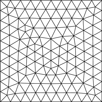
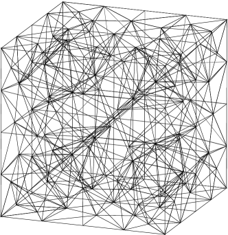
Figure 1. 2d triangular partition (left) / 3d tetrahedral partition (right).

Example 1. In the first example, we consider a smooth problem in two dimensions. On the domain $\Omega=(-1,1)^{2}$, we select the exact solution $u(x,y)$ and the smooth coefficient $A(x,y)$ as

$$u(x,y)=xy\sin(2\pi x)\sin(3\pi y),\quad(x,y)\text{ in }\Omega,$$

and

$$A(x,y)=\begin{bmatrix}|\sin(4\pi x)|^{1/5}+1&\cos(2xy\pi)\\ \cos(2xy\pi)&|\sin(4\pi y)|^{1/5}+1\\ \end{bmatrix}.$$

The source term and boundary condition are taken accordingly. We solve this problem on a sequence of triangular meshes with mesh size $h=1/10,1/20,\cdots,1/160$, see Fig 1 for the coarsest mesh. We employ the finite element spaces $\boldsymbol{\mathrm{S}}_{h}^{m}\times\widetilde{V}_{h}^{m}$ with $1\leq m\leq 3$ to seek numerical solutions $(\boldsymbol{p}_{h},u_{h})$ for approximating $(\boldsymbol{p},u)$ in (3). For the gradient, we plot the errors $\|\boldsymbol{p}-\boldsymbol{p}_{h}\|_{\boldsymbol{\mathrm{p}}}$ and $\|\boldsymbol{p}-\boldsymbol{p}_{h}\|_{L^{2}(\Omega)}$ in Fig 2. For fixed $m$, it is clear that the error $\|\boldsymbol{p}-\boldsymbol{p}_{h}\|_{\boldsymbol{\mathrm{p}}}$ converges to zero with the rate $O(h^{m})$ and error $\|\boldsymbol{p}-\boldsymbol{p}_{h}\|_{L^{2}(\Omega)}$ converges to zero with the rate $O(h^{m+1})$ as the mesh size decreases to zero. All convergence rates are optimal and coincide with the Theorem 26. For $u$, we plot the numerical errors in both $L^{2}$ norm and energy norm in Fig 3. We also attain the optimal convergence rates $O(h^{m})$ and $O(h^{m+1})$ for the errors $\|u-u_{h}\|_{\boldsymbol{\mathrm{u}}}$ and $\|u-u_{h}\|_{L^{2}(\Omega)}$, respectively. We note that all the convergence rates perfectly agree with the error estimates.

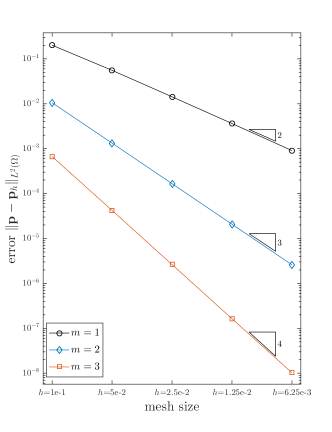
Figure 2. Example 1. The convergence rates of $\|\boldsymbol{p}-\boldsymbol{p}_{h}\|_{\boldsymbol{\mathrm{p}}}$ (left) / $\|\boldsymbol{p}-\boldsymbol{p}_{h}\|_{L^{2}(\Omega)}$ (right).

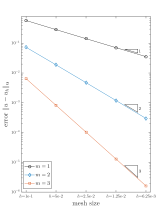
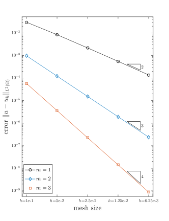
Figure 3. Example 1. The convergence rates of $\|u-u_{h}\|_{\boldsymbol{\mathrm{u}}}$ (left) / $\|u-u_{h}\|_{L^{2}(\Omega)}$ (right).

Example 2. In this example, we choose a discontinuous coefficients $A(x,y)$ which reads

$$A(x,y)=\begin{bmatrix}2&\frac{xy}{|xy|}\\ \frac{xy}{|xy|}&2\\ \end{bmatrix}.$$

The exact solution and the triangular meshes and the approximating spaces are taken as the same as in Example 1. The numerically convergence rates are displayed in Fig 4 and Fig 5. Clearly, for both variables $\boldsymbol{p}$ and $u$ the rates of convergence in $L^{2}$ norm and energy norm are $m+1$ and $m$, respectively, which again are in perfect agreement with theoretical results.

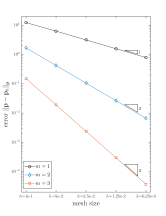
Figure 4. Example 2. The convergence rates of $\|\boldsymbol{p}-\boldsymbol{p}_{h}\|_{\boldsymbol{\mathrm{p}}}$ (left) / $\|\boldsymbol{p}-\boldsymbol{p}_{h}\|_{L^{2}(\Omega)}$ (right).

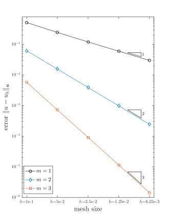
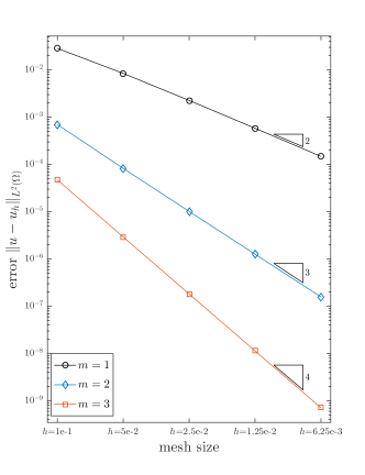
Figure 5. Example 2. The convergence rates of $\|u-u_{h}\|_{\boldsymbol{\mathrm{u}}}$ (left) / $\|u-u_{h}\|_{L^{2}(\Omega)}$ (right).

Example 3. This is a 3D example and we solve a problem in the unit cube $\Omega=(-1,1)^{3}$. We partition the domain $\Omega$ into a series of tetrahedral meshes with mesh size = $1/4$, $1/8$, $1/16$, $1/32$, see Fig 1 for the tetrahedral mesh with $h=1/4$. The analytical solution and the coefficient matrix are setup as

$$u(x,y,z)=\cos(2\pi x)\cos(2\pi y)\cos(2\pi z),$$

and

$$A(x,y,z)=\begin{bmatrix}10&\frac{xy}{|xy|}&\frac{xz}{|xz|}\\ \frac{yx}{|yx|}&10&\frac{yz}{|yz|}\\ \frac{zx}{|zx|}&\frac{zy}{|zy|}&10\\ \end{bmatrix},$$

and the boundary condition $g$ and the source term $f$ are taken suitably. We also use the finite element spaces $\boldsymbol{\mathrm{S}}_{h}^{m}\times\widetilde{V}_{h}^{m}$ with $1\leq m\leq 3$ to approximate $\boldsymbol{p}$ and $u$, respectively. The numerical results are shown in Fig 6 and Fig 7. All computed convergence orders agree with the theoretical results.

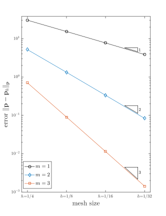
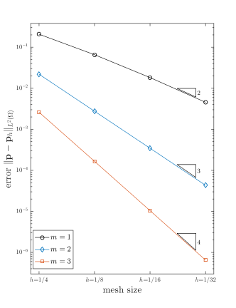
Figure 6. Example 3. The convergence rates of $\|\boldsymbol{p}-\boldsymbol{p}_{h}\|_{\boldsymbol{\mathrm{p}}}$ (left) / $\|\boldsymbol{p}-\boldsymbol{p}_{h}\|_{L^{2}(\Omega)}$ (right).

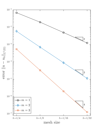
Figure 7. Example 3. The convergence rates of $\|u-u_{h}\|_{\boldsymbol{\mathrm{u}}}$ (left) / $\|u-u_{h}\|_{L^{2}(\Omega)}$ (right).

Example 4. In this example, we consider the problem on the domain $(0,1)^{2}$ and the exact solution is chosen to be

$$u(x,y)=|\boldsymbol{x}|^{\alpha},$$

where $\alpha$ is a positive constant. The coefficient matrix $A(x,y)$ takes the form

$$A(x,y)=\begin{bmatrix}1+x^{2}&xy\\ xy&1+y^{2}\\ \end{bmatrix},$$

and the data function $f$ and $g$ are selected properly. Notice that $u$ belongs to the space $H^{\alpha+1-\delta}(\Omega)$ for arbitrary small $\delta$. In the following, we take $\alpha=1.2$ to test the adaptive algorithm proposed in the previous section. The parameter $\theta$ is chosen $\theta=0.4$ and we consider the linear accuracy $\boldsymbol{\mathrm{S}}_{h}^{1}\times\widetilde{V}_{h}^{1}$ in the approximation to the variables $\boldsymbol{p}$ and $u$. The mesh size of initial triangular partition is taken as $h=0.1$, see left figure in Fig 1. The whole convergence history of the uniform refinement and adaptive refinement is displayed in Fig 8. For the uniform refinement, we observe the error $\|\boldsymbol{p}-\boldsymbol{p}_{h}\|_{\boldsymbol{\mathrm{p}}}$ decreases to zero at the speed $O(h^{0.2})$, which agrees with the convergence analysis. For the error $\|\boldsymbol{p}-\boldsymbol{p}_{h}\|_{L^{2}(\Omega)}$, the uniform refinement leads to a reduced convergence speed $O(h^{1})$. The reason may be traced to the singularity of $u$ at the corner. Furthermore, for $u$ the errors $\|u-u_{h}\|_{\boldsymbol{\mathrm{u}}}$ and $\|u-u_{h}\|_{L^{2}(\Omega)}$ approach to zero at the rate $O(h^{1})$, which matches with the theoretical analysis that the convergence rates in both norms for $u$ depend on the convergence rate of $\|\boldsymbol{p}-\boldsymbol{p}_{h}\|_{L^{2}(\Omega)}$. For the adaptive refinement, we note that all error measurements seem to be optimal. The triangular meshes after 6 adaptive refinement steps are shown in Fig 9. Clearly, the refinement is pronounced in the regions where the solution is of low regularity.

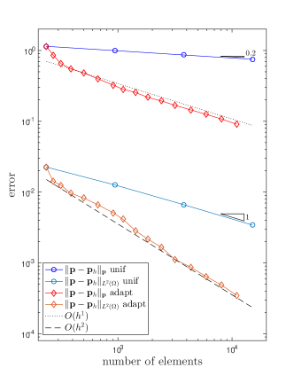
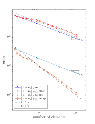
Figure 8. Example 4. The convergence history of $\boldsymbol{p}$ (left) / $u$ (right).

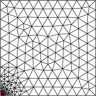
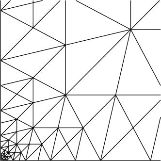
Figure 9. Triangular mesh after 6 adaptive refinement steps (left) / elements in the red rectangle (right).

6. Conclusion

We proposed a sequential least squares finite element method for elliptic equations in non-divergence form. We employed a novel piecewise curl-free approximate space to solve the gradient variable first and then we solve the primitive variable in the $C^{0}$ finite element space. We proved the convergence rates for both variables with respect to the $L^{2}$ norm and the energy norm. Optimal convergence orders for all measurements were detected in numerical experiments. We also tried an adaptive algorithm using $h$-adaptive method to improve numerical efficiency for a problem of low regularity.

References

- [1] D. N. Arnold, F. Brezzi, B. Cockburn, and L. D. Marini, Unified analysis of discontinuous Galerkin methods for elliptic problems, SIAM J. Numer. Anal. 39 (2001/02), no. 5, 1749–1779.
- [2] Ivo Babuška, Gabriel Caloz, and John E. Osborn, Special finite element methods for a class of second order elliptic problems with rough coefficients, SIAM J. Numer. Anal. 31 (1994), no. 4, 945–981.
- [3] Rickard E. Bensow and Mats G. Larson, Discontinuous/continuous least-squares finite element methods for elliptic problems, Math. Models Methods Appl. Sci. 15 (2005), no. 6, 825–842.
- [4] Bernard Bialecki, Convergence analysis of orthogonal spline collocation for elliptic boundary value problems, SIAM J. Numer. Anal. 35 (1998), no. 2, 617–631.
- [5] Pavel B. Bochev and Max D. Gunzburger, Finite element methods of least-squares type, SIAM Rev. 40 (1998), no. 4, 789–837.
- [6] Klaus Böhmer, On finite element methods for fully nonlinear elliptic equations of second order, SIAM J. Numer. Anal. 46 (2008), no. 3, 1212–1249.
- [7] Luis A. Caffarelli and Cristian E. Gutiérrez, Properties of the solutions of the linearized Monge-Ampère equation, Amer. J. Math. 119 (1997), no. 2, 423–465.
- [8] Xiaobing Feng, Lauren Hennings, and Michael Neilan, Finite element methods for second order linear elliptic partial differential equations in non-divergence form, Math. Comp. 86 (2017), no. 307, 2025–2051.
- [9] Xiaobing Feng and Michael Neilan, Mixed finite element methods for the fully nonlinear Monge-Ampère equation based on the vanishing moment method, SIAM J. Numer. Anal. 47 (2009), no. 2, 1226–1250.
- [10] Dietmar Gallistl, Variational formulation and numerical analysis of linear elliptic equations in nondivergence form with Cordes coefficients, SIAM J. Numer. Anal. 55 (2017), no. 2, 737–757.
- [11] Dietmar Gallistl and Endre Süli, Mixed finite element approximation of the Hamilton-Jacobi-Bellman with Cordes coefficients, SIAM J. Numer. Anal. 57 (2019), no. 2, 592–614.
- [12] Vivette Girault and Pierre Arnaud Raviart, Finite element methods for navier-stokes equations: Theory and algorithms, Springer-Verlag, 1986.
- [13] Ohannes A. Karakashian and Frederic Pascal, Convergence of adaptive discontinuous Galerkin approximations of second-order elliptic problems, SIAM J. Numer. Anal. 45 (2007), no. 2, 641–665.
- [14] Omar Lakkis and Tristan Pryer, A finite element method for second order nonvariational elliptic problems, SIAM J. Sci. Comput. 33 (2011), no. 2, 786–801.
- [15] Ruo Li and Fanyi Yang, A sequential least squares method for Poisson equation using a patch reconstructed space, SIAM J. Numer. Anal. 58 (2020), no. 1, 353–374.
- [16] Jiangguo Liu and Rachel Cali, A note on the approximation properties of the locally divergence-free finite elements, Int. J. Numer. Anal. Model. 5 (2008), no. 4, 693–703.
- [17] Michael Neilan and Mohan Wu, Discrete Miranda-Talenti estimates and applications to linear and nonlinear PDEs, J. Comput. Appl. Math. 356 (2019), 358–376.
- [18] Iain Smears and Endre Süli, Discontinuous Galerkin finite element approximation of nondivergence form elliptic equations with Cordès coefficients, SIAM J. Numer. Anal. 51 (2013), no. 4, 2088–2106.
- [19] by same author, Discontinuous Galerkin finite element approximation of Hamilton-Jacobi-Bellman equations with Cordes coefficients, SIAM J. Numer. Anal. 52 (2014), no. 2, 993–1016.
- [20] Chunmei Wang and Junping Wang, A primal-dual weak Galerkin finite element method for second order elliptic equations in non-divergence form, Math. Comp. 87 (2018), no. 310, 515–545.