Randomization and reweighted $\ell_{1}$-minimization for A-optimal design of linear inverse problems

Abstract

We consider optimal design of PDE-based Bayesian linear inverse problems with infinite-dimensional parameters. We focus on the A-optimal design criterion, defined as the average posterior variance and quantified by the trace of the posterior covariance operator. We propose using structure exploiting randomized methods to compute the A-optimal objective function and its gradient, and provide a detailed analysis of the error for the proposed estimators. To ensure sparse and binary design vectors, we develop a novel reweighted $\ell_{1}$-minimization algorithm. We also introduce a modified A-optimal criterion and present randomized estimators for its efficient computation. We present numerical results illustrating the proposed methods on a model contaminant source identification problem, where the inverse problem seeks to recover the initial state of a contaminant plume using discrete measurements of the contaminant in space and time.

35R30; 62K05; 68W20; 35Q62; 65C60; 62F15.

1 Introduction

A central problem in scientific computing involves estimating parameters that describe mathematical models, such as initial conditions, boundary conditions, or material parameters. This is often addressed by using experimental measurements and a mathematical model to compute estimates of unknown model parameters. In other words, one can estimate the parameters by solving an inverse problem. Experimental design involves specifying the experimental setup for collecting measurement data, with the goal of accurately recovering the parameters of interest. As such, optimal experimental design (OED) is an important aspect of effective and efficient parameter estimation. Namely, in applications where collecting experimental measurements is expensive (e.g., because of budget, labor, or physical constraints), deploying experimental resources has to be done efficiently and in a parsimonious manner. Even when collecting large amounts of data is feasible, OED is still important; the computational cost of processing all the data may be prohibitive or a poorly designed experiment with many measurements may miss important information about the parameters of interest.

To make matters concrete, we explain the inverse problem and the experimental design in the context of an application. Consider the transport of a contaminant in an urban environment or the subsurface. The forward problem involves forecasting the spread of the contaminant, whereas the inverse problem involves using the measurements of the contaminant concentration at discrete points in space and time to recover the source of the contaminant (i.e., the initial state). In this application, OED involves optimal placement of sensors, at which measurement data is collected, to reconstruct the initial state.

We focus on OED for Bayesian linear inverse problems governed by PDEs. In our formulation of the OED problem, the goal is to find an optimal subset of sensors from a fixed array of ${n_{s}}$ candidate sensor sites. The experimental design is parameterized by assigning non-negative weights to each candidate sensor location. Ideally, we seek a binary weight vector $\textstyle{w}$; if $w_{i}=1$, a sensor will be placed at the $i$th candidate location, and if $w_{i}=0$, no sensor will be placed at the location. However, formulating an optimization problem over binary weight vectors leads to a problem with combinatorial complexity that is computationally prohibitive. A common approach to address this issue is to relax the binary requirement on design weights by letting the weights take values in the interval $[0,1]$. The sparsity of the design will then be controlled using a penalty method; see e.g., [13, 2, 23]. This results in an optimization problem of the following form:

(1) $$\min_{{\mathchoice{\mbox{\boldmath$\displaystyle{w}$}}{\mbox{\boldmath$\textstyle{w}$}}{\mbox{\boldmath$\scriptstyle{w}$}}{\mbox{\boldmath$\scriptscriptstyle{w}$}}}\in[0,1]^{n_{s}}}\Phi({\mathchoice{\mbox{\boldmath$\displaystyle{w}$}}{\mbox{\boldmath$\textstyle{w}$}}{\mbox{\boldmath$\scriptstyle{w}$}}{\mbox{\boldmath$\scriptscriptstyle{w}$}}})+\gamma P({\mathchoice{\mbox{\boldmath$\displaystyle{w}$}}{\mbox{\boldmath$\textstyle{w}$}}{\mbox{\boldmath$\scriptstyle{w}$}}{\mbox{\boldmath$\scriptscriptstyle{w}$}}}),$$

where $\Phi$ denotes the design criterion, $\gamma>0$ is a penalty parameter, and $P$ is a penalty function.

Adopting a Bayesian approach to the inverse problem, the design criterion will be a measure of the uncertainty in the estimated parameters. In this article, we focus on a popular choice known as the A-optimal criterion [22, 8]. That is, we seek a sensor configuration that results in a minimized average posterior variance. The design criterion, in this case, is given by the trace of the posterior covariance operator.

One major challenge in solving Eq. 1, specifically for PDE-based inverse problems, is the computational cost of objective function and gradient evaluations. Namely, the posterior covariance operator $\mathbf{\Gamma}_{\text{post}}$ is dense, high-dimensional, and computationally challenging to explicitly form—computing applications of $\mathbf{\Gamma}_{\text{post}}$ to vectors requires solving multiple PDEs. Furthermore, these computations must be performed at each iteration of an optimization algorithm used to solve Eq. 1. To address this computational challenge, efficient and accurate matrix-free approaches for computing the OED objective and its gradient are needed. Another challenge in solving the OED problem Eq. 1 is the need for a suitable penalty method that is computationally tractable and results in sparse and binary optimal weight vectors. This article is about methods for overcoming these computational challenges.

Related work

For an extensive review of the OED literature, we refer the reader to [3]. We focus here on works that are closely related to the present article. Algorithms for A-optimal designs for ill-posed linear inverse problems were proposed in [11, 13, 10] and more specifically for infinite-dimensional Bayesian linear inverse problems in [2]. In majority of these articles, Monte-Carlo trace estimators are used to approximate the A-optimal design criterion and its gradient. Also, [13, 2] advocate use of low-rank approximations using the Lanczos algorithm or the randomized SVD [14]. We refer to our previous work [20] for comparison of Monte Carlo trace estimators and those based on randomized subspace iteration; it was shown that the latter are significantly more accurate than Monte Carlo trace estimators. Regarding sparsity control, various techniques have been used to approximate the $\ell_{0}$-“norm” to enforce sparse and binary designs. For example, [11, 12, 13] use the $\ell_{1}$-penalty function with an appropriate threshold to post-process the solution. In [2], a continuation approach is proposed that involves solving a sequence of optimization problems with non-convex penalty functions that approximate the $\ell_{0}$-“norm”. More recently, in [23], a sum-up rounding approach is proposed to obtain binary optimal designs.

Our approach and contributions

In this article, we make the following advances in methods for A-optimal sensor placements in infinite-dimensional Bayesian linear inverse problems:

1. We present efficient and accurate randomized estimators of the A-optimal criterion and its gradient, based on randomized subspace iteration. This is accompanied by a detailed algorithm that guides efficient implementations, discussion of computational cost, as well as theoretical error analysis; see Section 3. Our estimators are structure exploiting, in that they use the low-rank structure embedded in the posterior covariance operator. To quantify the accuracy of the estimators we present rigorous error analysis, significantly advancing the methods in [20]. A desirable feature of our analysis is that the bounds are independent of the dimension of the discretized inversion parameter. Furthermore, the computational cost (measured in the number of PDE solves) of the A-optimal objective and gradient using our proposed estimators is independent of the discretized parameter dimension.

2. We propose a new algorithm for optimal sensor placement that is based on solving a sequence of reweighted $\ell_{1}$-optimization problems; see Section 4. An important benefit of this approach is that one works with convex penalty functions, and since the A-optimal criterion itself is a convex function of $\textstyle{w}$, in each step of the reweighted $\ell_{1}$ algorithm a convex optimization problem is solved. We derive this algorithm by using the Majorization-Minimization principle applied to a novel penalty function that promotes binary designs. The solution of the reweighted $\ell_{1}$-optimization problems is accelerated by the efficient randomized estimators for the optimality criterion and its gradient. To our knowledge, the presented framework, based on reweighted $\ell_{1}$-minimization, is the first of its kind in the context of OED.

3. Motivated by reducing computational cost, we propose a new criterion known as modified A-optimal criterion; see Section 5. This criterion is derived by considering a suitably weighted A-optimal criterion. We present randomized estimators with complete error analysis for computing the modified A-optimal criterion and its gradient.

We illustrate the benefits of the proposed algorithms on a model problem from contaminant source identification. A comprehensive set of numerical experiments is provided so to test various aspect of the presented approach; see Section 6.

Finally, we remark that the randomized estimators and the reweighted $\ell_{1}$ approach for promoting sparse and binary weights are of independent interest beyond the application to OED.

2 Preliminaries

In this section, we recall the background material needed in the remainder of the article.

2.1 Bayesian linear inverse problems

We consider a linear inverse problem of estimating $m$, using the model

$$Fm+{\mathchoice{\mbox{\boldmath$\displaystyle{\eta}$}}{\mbox{\boldmath$\textstyle{\eta}$}}{\mbox{\boldmath$\scriptstyle{\eta}$}}{\mbox{\boldmath$\scriptscriptstyle{\eta}$}}}={\mathchoice{\mbox{\boldmath$\displaystyle{y}$}}{\mbox{\boldmath$\textstyle{y}$}}{\mbox{\boldmath$\scriptstyle{y}$}}{\mbox{\boldmath$\scriptscriptstyle{y}$}}}.$$

Here $F$ is a linear parameter-to-observable map (also called the forward operator), $\textstyle{\eta}$ represents the measurement noise, and $\textstyle{y}$ is a vector of measurement data. The inversion parameter $m$ is an element of $\mathcal{V}=L^{2}(\mathcal{D})$, where $\mathcal{D}$ is a bounded domain.

The setup of the inverse problem

To fully specify the inverse problem, we need to describe the prior law of $m$ and our choice of data likelihood. For the prior, we choose a Gaussian measure $\mu_{\mathup{pr}}=\mathcal{N}({m_{\mathup{pr}}},{\Gamma_{\mathup{pr}}})$. We assume the prior mean $m_{\mathup{pr}}$ is a sufficiently regular element of $\mathcal{V}$ and that the covariance operator $\Gamma_{\mathup{pr}}:\mathcal{V}\to\mathcal{V}$ is a strictly positive self-adjoint trace-class operator. Following the developments in [21, 6, 9], we use $\Gamma_{\mathup{pr}}=\mathcal{A}^{-2}$ with $\mathcal{A}$ taken to be a Laplacian-like operator [21]. This ensures that $\Gamma_{\mathup{pr}}$ is trace-class in two and three space dimensions.

We consider the case where $F$ represents a time-dependent PDE and we assume observations are taken at ${n_{s}}$ sensor locations at ${n_{t}}$ points in time. Thus, the vector of experimental data $\textstyle{y}$ is an element of $\mathbb{R}^{{n_{s}}{n_{t}}}$. An application of the parameter-to-observable map, $F:\mathcal{V}\to\mathbb{R}^{{n_{s}}{n_{t}}}$, involves a PDE solve followed by an application of a spatiotemporal observation operator. We assume a Gaussian distribution on the experimental noise, ${\mathchoice{\mbox{\boldmath$\displaystyle{\eta}$}}{\mbox{\boldmath$\textstyle{\eta}$}}{\mbox{\boldmath$\scriptstyle{\eta}$}}{\mbox{\boldmath$\scriptscriptstyle{\eta}$}}}\sim\mathcal{N}({{\mathchoice{\mbox{\boldmath$\displaystyle{0}$}}{\mbox{\boldmath$\textstyle{0}$}}{\mbox{\boldmath$\scriptstyle{0}$}}{\mbox{\boldmath$\scriptscriptstyle{0}$}}}},{{\mathchoice{\mbox{\boldmath$\displaystyle{\Gamma}$}}{\mbox{\boldmath$\textstyle{\Gamma}$}}{\mbox{\boldmath$\scriptstyle{\Gamma}$}}{\mbox{\boldmath$\scriptscriptstyle{\Gamma}$}}}_{\!\mathup{noise}}})$. Given this choice of the noise model—additive and Gaussian—the likelihood probability density function (pdf) is

$$\pi_{\mathup{like}}({\mathchoice{\mbox{\boldmath$\displaystyle{y}$}}{\mbox{\boldmath$\textstyle{y}$}}{\mbox{\boldmath$\scriptstyle{y}$}}{\mbox{\boldmath$\scriptscriptstyle{y}$}}}\mid m)\propto\exp\left\{-\frac{1}{2}\big{(}Fm-{\mathchoice{\mbox{\boldmath$\displaystyle{y}$}}{\mbox{\boldmath$\textstyle{y}$}}{\mbox{\boldmath$\scriptstyle{y}$}}{\mbox{\boldmath$\scriptscriptstyle{y}$}}}\big{)}^{\top}{\mathchoice{\mbox{\boldmath$\displaystyle{\Gamma}$}}{\mbox{\boldmath$\textstyle{\Gamma}$}}{\mbox{\boldmath$\scriptstyle{\Gamma}$}}{\mbox{\boldmath$\scriptscriptstyle{\Gamma}$}}}_{\!\mathup{noise}}^{-1}\big{(}Fm-{\mathchoice{\mbox{\boldmath$\displaystyle{y}$}}{\mbox{\boldmath$\textstyle{y}$}}{\mbox{\boldmath$\scriptstyle{y}$}}{\mbox{\boldmath$\scriptscriptstyle{y}$}}}\big{)}\right\}.$$

Furthermore, the solution of the Bayesian inverse problem—the posterior distribution law $\mu_{\mathup{post}}^{{{\mathchoice{\mbox{\boldmath$\displaystyle{y}$}}{\mbox{\boldmath$\textstyle{y}$}}{\mbox{\boldmath$\scriptstyle{y}$}}{\mbox{\boldmath$\scriptscriptstyle{y}$}}}}}$—is given by the Gaussian measure $\mu_{\mathup{post}}^{{{\mathchoice{\mbox{\boldmath$\displaystyle{y}$}}{\mbox{\boldmath$\textstyle{y}$}}{\mbox{\boldmath$\scriptstyle{y}$}}{\mbox{\boldmath$\scriptscriptstyle{y}$}}}}}=\mathcal{N}({m_{\mathup{post}}^{\mathchoice{\mbox{\boldmath$\displaystyle{y}$}}{\mbox{\boldmath$\textstyle{y}$}}{\mbox{\boldmath$\scriptstyle{y}$}}{\mbox{\boldmath$\scriptscriptstyle{y}$}}}},{\Gamma_{\mathup{post}}})$ with

(2) $$m_{\mathup{post}}^{\mathchoice{\mbox{\boldmath$\displaystyle{y}$}}{\mbox{\boldmath$\textstyle{y}$}}{\mbox{\boldmath$\scriptstyle{y}$}}{\mbox{\boldmath$\scriptscriptstyle{y}$}}}=\Gamma_{\mathup{post}}(F^{*}{\mathchoice{\mbox{\boldmath$\displaystyle{\Gamma}$}}{\mbox{\boldmath$\textstyle{\Gamma}$}}{\mbox{\boldmath$\scriptstyle{\Gamma}$}}{\mbox{\boldmath$\scriptscriptstyle{\Gamma}$}}}_{\!\mathup{noise}}^{-1}{\mathchoice{\mbox{\boldmath$\displaystyle{y}$}}{\mbox{\boldmath$\textstyle{y}$}}{\mbox{\boldmath$\scriptstyle{y}$}}{\mbox{\boldmath$\scriptscriptstyle{y}$}}}+\Gamma_{\mathup{pr}}^{-1}m_{\mathup{pr}}),\qquad\Gamma_{\mathup{post}}=(F^{*}{\mathchoice{\mbox{\boldmath$\displaystyle{\Gamma}$}}{\mbox{\boldmath$\textstyle{\Gamma}$}}{\mbox{\boldmath$\scriptstyle{\Gamma}$}}{\mbox{\boldmath$\scriptscriptstyle{\Gamma}$}}}_{\!\mathup{noise}}^{-1}F+\Gamma_{\mathup{pr}}^{-1})^{-1}.$$

Note that here the posterior mean $m_{\mathup{post}}^{\mathchoice{\mbox{\boldmath$\displaystyle{y}$}}{\mbox{\boldmath$\textstyle{y}$}}{\mbox{\boldmath$\scriptstyle{y}$}}{\mbox{\boldmath$\scriptscriptstyle{y}$}}}$ coincides with the maximum a posteriori probability (MAP) estimator. We refer to [21] for further details.

Discretization

We use a continuous Galerkin finite element discretization approach for the governing PDEs, as well as the inverse problem. Specifically, our discretization of the Bayesian inverse problem follows the developments in [6]. The discretized parameter space in the present case is $\mathcal{V}_{n}=\mathbb{R}^{n}$ equipped with the inner product $\langle{\cdot},{\cdot}\rangle_{\scriptscriptstyle{\mathbf{M}}}$ and norm $\|{\cdot}\|_{\scriptscriptstyle{\mathbf{M}}}=\langle{\cdot},{\cdot}\rangle_{\scriptscriptstyle{\mathbf{M}}}^{1/2}$, where $\mathbf{M}$ is the finite element mass matrix. Note that $\langle{\cdot},{\cdot}\rangle_{\scriptscriptstyle{\mathbf{M}}}$ is the discretized $L^{2}(\mathcal{D})$ inner product. The discretized parameter-to-observable map is a linear transformation $\mathbf{F}:\mathcal{V}_{n}\to\mathbb{R}^{{n_{s}}{n_{t}}}$ with adjoint $\mathbf{F}^{*}$ discussed below. The discretized prior measure $\mathcal{N}({{\mathchoice{\mbox{\boldmath$\displaystyle{m}$}}{\mbox{\boldmath$\textstyle{m}$}}{\mbox{\boldmath$\scriptstyle{m}$}}{\mbox{\boldmath$\scriptscriptstyle{m}$}}}_{\mathup{pr}}},{\mathbf{\Gamma}_{\text{pr}}})$ is obtained by discretizing the prior mean and covariance operator, and the discretized posterior measure is given by $\mathcal{N}({{\mathchoice{\mbox{\boldmath$\displaystyle{m}$}}{\mbox{\boldmath$\textstyle{m}$}}{\mbox{\boldmath$\scriptstyle{m}$}}{\mbox{\boldmath$\scriptscriptstyle{m}$}}}_{\text{post}}},{\mathbf{\Gamma}_{\text{post}}})$, with

$$\mathbf{\Gamma}_{\text{post}}=\left(\mathbf{F}^{*}{\mathchoice{\mbox{\boldmath$\displaystyle{\Gamma}$}}{\mbox{\boldmath$\textstyle{\Gamma}$}}{\mbox{\boldmath$\scriptstyle{\Gamma}$}}{\mbox{\boldmath$\scriptscriptstyle{\Gamma}$}}}^{-1}_{\text{noise}}\mathbf{F}+\mathbf{\Gamma}^{-1}_{\text{pr}}\right)^{-1},\quad{\mathchoice{\mbox{\boldmath$\displaystyle{m}$}}{\mbox{\boldmath$\textstyle{m}$}}{\mbox{\boldmath$\scriptstyle{m}$}}{\mbox{\boldmath$\scriptscriptstyle{m}$}}}_{\mathup{post}}^{\mathchoice{\mbox{\boldmath$\displaystyle{y}$}}{\mbox{\boldmath$\textstyle{y}$}}{\mbox{\boldmath$\scriptstyle{y}$}}{\mbox{\boldmath$\scriptscriptstyle{y}$}}}=\mathbf{\Gamma}_{\text{post}}\left(\mathbf{F}^{*}{\mathchoice{\mbox{\boldmath$\displaystyle{\Gamma}$}}{\mbox{\boldmath$\textstyle{\Gamma}$}}{\mbox{\boldmath$\scriptstyle{\Gamma}$}}{\mbox{\boldmath$\scriptscriptstyle{\Gamma}$}}}^{-1}_{\text{noise}}{\mathchoice{\mbox{\boldmath$\displaystyle{y}$}}{\mbox{\boldmath$\textstyle{y}$}}{\mbox{\boldmath$\scriptstyle{y}$}}{\mbox{\boldmath$\scriptscriptstyle{y}$}}}+\mathbf{\Gamma}^{-1}_{\text{pr}}{\mathchoice{\mbox{\boldmath$\displaystyle{m}$}}{\mbox{\boldmath$\textstyle{m}$}}{\mbox{\boldmath$\scriptstyle{m}$}}{\mbox{\boldmath$\scriptscriptstyle{m}$}}}_{\text{pr}}\right).$$

We point out that the operator $\mathbf{F}^{*}{\mathchoice{\mbox{\boldmath$\displaystyle{\Gamma}$}}{\mbox{\boldmath$\textstyle{\Gamma}$}}{\mbox{\boldmath$\scriptstyle{\Gamma}$}}{\mbox{\boldmath$\scriptscriptstyle{\Gamma}$}}}^{-1}_{\text{noise}}\mathbf{F}$ is the Hessian of the data-misfit cost functional whose minimizer is the MAP point, and is thus referred to as the data-misfit Hessian; see e.g., [2].

It is important to keep track of the inner products in the domains and ranges of the linear mappings, appearing in the above expressions, when computing the respective adjoint operators. For the readers’ convenience, in Fig. 1, we summarize the different spaces that are important, the respective inner products, and the adjoints of the linear transformations defined between these spaces.

Figure 1: Different spaces, their inner products, and the adjoints of linear transformations between them. Here $\langle{\cdot},{\cdot}\rangle$ denotes the Euclidean inner product and $\langle{\cdot},{\cdot}\rangle_{\scriptscriptstyle{\mathbf{M}}}$ is the mass-weighted inner product.

Using the fact that $\mathbf{\Gamma}_{\text{pr}}$ is a self-adjoint operator on $\mathcal{V}_{n}$ and the form of the adjoint operator $\mathbf{F}^{*}$ (see Fig. 1), we can rewrite the expression for $\mathbf{\Gamma}_{\text{post}}$ as follows:

$$\mathbf{\Gamma}_{\text{post}}=\mathbf{\Gamma}^{1/2}_{\text{pr}}\mathbf{M}^{-1/2}\left(\mathbf{I}+{\mathbfcal{F}}^{\top}{{\mathchoice{\mbox{\boldmath$\displaystyle{\Gamma}$}}{\mbox{\boldmath$\textstyle{\Gamma}$}}{\mbox{\boldmath$\scriptstyle{\Gamma}$}}{\mbox{\boldmath$\scriptscriptstyle{\Gamma}$}}}}_{\text{noise}}^{-1}{\mathbfcal{F}}\right)^{-1}\mathbf{M}^{1/2}\mathbf{\Gamma}^{1/2}_{\text{pr}},$$

with

(3) $${\mathbfcal{F}}=\mathbf{F}\mathbf{\Gamma}^{1/2}_{\text{pr}}\mathbf{M}^{-1/2}.$$

Note that the operator $\mathbfcal{H}_{\text{m}}={\mathbfcal{F}}^{\top}{{\mathchoice{\mbox{\boldmath$\displaystyle{\Gamma}$}}{\mbox{\boldmath$\textstyle{\Gamma}$}}{\mbox{\boldmath$\scriptstyle{\Gamma}$}}{\mbox{\boldmath$\scriptscriptstyle{\Gamma}$}}}}_{\text{noise}}^{-1}{\mathbfcal{F}}$ is a symmetric positive semidefinite matrix, and is a similarity transform of the prior-preconditioned data-misfit Hessian $\mathbf{\Gamma}^{1/2}_{\text{pr}}\mathbf{F}^{*}{\mathchoice{\mbox{\boldmath$\displaystyle{\Gamma}$}}{\mbox{\boldmath$\textstyle{\Gamma}$}}{\mbox{\boldmath$\scriptstyle{\Gamma}$}}{\mbox{\boldmath$\scriptscriptstyle{\Gamma}$}}}^{-1}_{\text{noise}}\mathbf{F}\mathbf{\Gamma}^{1/2}_{\text{pr}}$. In many applications (including the application considered in Section 6), $\mathbfcal{H}_{\text{m}}$ has rapidly decaying eigenvalues and therefore, it can be approximated by a low-rank matrix. This is a key insight that will be exploited in our estimators for the OED criterion and its gradient.

2.2 Randomized subspace iteration algorithm

In this article, we develop and use randomized estimators to efficiently compute the design criteria and their derivatives. We first explain how to use randomized algorithms for computing low-rank approximations of a symmetric positive semidefinite matrix $\mathbf{A}\in\mathbb{R}^{n\times n}$. To draw connection with the previous subsection, in our application $\mathbf{A}$ will stand for $\mathbfcal{H}_{\text{m}}$. We first draw a random Gaussian matrix $\boldsymbol{\Omega}\in\mathbb{R}^{n\times\ell}$ (i.e., the entries are independent and identically distributed standard normal random variables). We then perform $q$ steps of subspace iteration on $\mathbf{A}$ with the starting guess $\boldsymbol{\Omega}$ to obtain the matrix $\mathbf{Y}$. If, for example, the matrix has rank $k\leq\ell$, or the eigenvalues decay sufficiently, then the range of $\mathbf{Y}$ is a good approximation to the range of $\mathbf{A}$ under these suitable conditions. This is the main insight behind randomized algorithms. We now show how to obtain a low-rank approximation of $\mathbf{A}$. A thin-QR factorization of $\mathbf{Y}$ is performed to obtain the matrix $\mathbf{Q}$, which has orthonormal columns. We then form the “projected” matrix $\mathbf{T}=\mathbf{Q}^{\top}\mathbf{A}\mathbf{Q}$ and obtain the low-rank approximation

(4) $$\mathbf{A}\approx\mathbf{Q}\mathbf{T}\mathbf{Q}^{\top}.$$

This low-rank approximation can be manipulated in many ways depending on the desired application. An alternative low-rank approximation can be computed using the Nyström approximation, see e.g., [14].

Algorithm 1 Randomized subspace iteration.

0:  $\mathbf{A}\in\mathbb{R}^{n\times n}$ with target rank $k$, oversampling parameter $p\geq 2$, with $\ell\equiv k+p\leq n$, and $q\geq 1$ (number of subspace iterations).

0:  $\mathbf{Q}\in\mathbb{R}^{n\times\ell},\mathbf{T}\in\mathbb{R}^{\ell\times\ell}$.

  Draw a standard Gaussian random matrix $\boldsymbol{\Omega}\in\mathbb{R}^{n\times\ell}$.

  Compute $\mathbf{Y}=\mathbf{A}^{q}\boldsymbol{\Omega}$.

  Compute thin QR decomposition $\mathbf{Y}=\mathbf{Q}\mathbf{R}.$

  Compute $\mathbf{T}=\mathbf{Q}^{\top}\mathbf{A}\mathbf{Q}$.

In addition, once the matrix $\mathbf{T}$ is computed, it can be used in various ways. In [20], $\mathsf{tr}\,\left(\mathbf{T}\right)$ was used as an estimator for $\mathsf{tr}\,\left(\mathbf{A}\right)$, whereas $\log\det(\mathbf{I}+\mathbf{T})$ was used as estimator for $\log\det(\mathbf{I}+\mathbf{A})$. The main idea behind these estimators is that the eigenvalues of $\mathbf{T}$ are good approximations to the eigenvalues of $\mathbf{A}$, when $\mathbf{A}$ is sufficiently low-rank or has rapidly decaying eigenvalues. Our estimators for the A-optimal criterion and its gradient utilize the same idea but in a slightly different form.

2.3 A-optimal design of experiments

As mentioned in the introduction, an experimental design refers to a placement of sensors used to collect measurement data for the purposes of parameter inversion. Here we describe the basic setup of the optimization problem for finding an A-optimal design.

Experimental design and A-optimal criterion

We seek to find an optimal subset of a network of ${n_{s}}$ candidate sensor locations, which collect measurements at ${n_{t}}$ points in time. The experimental design is parameterized by a vector of design weights ${\mathchoice{\mbox{\boldmath$\displaystyle{w}$}}{\mbox{\boldmath$\textstyle{w}$}}{\mbox{\boldmath$\scriptstyle{w}$}}{\mbox{\boldmath$\scriptscriptstyle{w}$}}}\in[0,1]^{n_{s}}$. In the present work, we use the A-optimal criterion to find the optimal design. That is, we seek designs that minimize the average posterior variance, as quantified by $\mathsf{tr}\,\left(\mathbf{\Gamma}_{\text{post}}({\mathchoice{\mbox{\boldmath$\displaystyle{w}$}}{\mbox{\boldmath$\textstyle{w}$}}{\mbox{\boldmath$\scriptstyle{w}$}}{\mbox{\boldmath$\scriptscriptstyle{w}$}}})\right)$. (The precise nature of the dependence of $\mathbf{\Gamma}_{\text{post}}$ on $\textstyle{w}$ will be explained below.) Note that $\mathsf{tr}\,\left(\mathbf{\Gamma}_{\text{post}}({\mathchoice{\mbox{\boldmath$\displaystyle{w}$}}{\mbox{\boldmath$\textstyle{w}$}}{\mbox{\boldmath$\scriptstyle{w}$}}{\mbox{\boldmath$\scriptscriptstyle{w}$}}})\right)=\mathsf{tr}\,\left(\mathbf{\Gamma}_{\text{post}}({\mathchoice{\mbox{\boldmath$\displaystyle{w}$}}{\mbox{\boldmath$\textstyle{w}$}}{\mbox{\boldmath$\scriptstyle{w}$}}{\mbox{\boldmath$\scriptscriptstyle{w}$}}})-\mathbf{\Gamma}_{\text{pr}}\right)+\mathsf{tr}\,\left(\mathbf{\Gamma}_{\text{pr}}\right)$ and thus, minimizing the trace of the posterior covariance operator is equivalent to minimizing

(5) $$\Phi_{\text{aopt}}{(}{\mathchoice{\mbox{\boldmath$\displaystyle{w}$}}{\mbox{\boldmath$\textstyle{w}$}}{\mbox{\boldmath$\scriptstyle{w}$}}{\mbox{\boldmath$\scriptscriptstyle{w}$}}})\equiv\mathsf{tr}\,\left(\mathbf{\Gamma}_{\text{post}}({\mathchoice{\mbox{\boldmath$\displaystyle{w}$}}{\mbox{\boldmath$\textstyle{w}$}}{\mbox{\boldmath$\scriptstyle{w}$}}{\mbox{\boldmath$\scriptscriptstyle{w}$}}})-\mathbf{\Gamma}_{\text{pr}}\right).$$

This is the objective function we seek to minimize for finding A-optimal designs. As seen below, this formulation of the A-optimal criterion is well suited for approximations via randomized matrix methods Section 2.2. Note also that minimizing $\Phi_{\text{aopt}}{(}{\mathchoice{\mbox{\boldmath$\displaystyle{w}$}}{\mbox{\boldmath$\textstyle{w}$}}{\mbox{\boldmath$\scriptstyle{w}$}}{\mbox{\boldmath$\scriptscriptstyle{w}$}}})$ amounts to maximizing $\mathsf{tr}\,\left(\mathbf{\Gamma}_{\text{pr}}\right)-\mathsf{tr}\,\left(\mathbf{\Gamma}_{\text{post}}({\mathchoice{\mbox{\boldmath$\displaystyle{w}$}}{\mbox{\boldmath$\textstyle{w}$}}{\mbox{\boldmath$\scriptstyle{w}$}}{\mbox{\boldmath$\scriptscriptstyle{w}$}}})\right)$, which can be thought of as a measure of uncertainty reduction.

We can also understand Eq. 5 from a decision theoretic point of view. It is well known [8, 1, 4] that for Bayesian linear inverse problems with Gaussian prior and additive Gaussian noise models, $\mathsf{tr}\,\left(\mathbf{\Gamma}_{\text{post}}{}\right)$ coincides with Bayes risk (with respect to the $L^{2}$ loss function):

$$\mathsf{tr}\,\left(\mathbf{\Gamma}_{\text{post}}{}\right)= \>\mathbb{E}_{\mu_{\mathup{pr}}}\Big{(}\mathbb{E}_{\pi_{\mathup{like}}({\mathchoice{\mbox{\boldmath$\displaystyle{y}$}}{\mbox{\boldmath$\textstyle{y}$}}{\mbox{\boldmath$\scriptstyle{y}$}}{\mbox{\boldmath$\scriptscriptstyle{y}$}}}\mid{\mathchoice{\mbox{\boldmath$\displaystyle{m}$}}{\mbox{\boldmath$\textstyle{m}$}}{\mbox{\boldmath$\scriptstyle{m}$}}{\mbox{\boldmath$\scriptscriptstyle{m}$}}})}\big{(}\|{{\mathchoice{\mbox{\boldmath$\displaystyle{m}$}}{\mbox{\boldmath$\textstyle{m}$}}{\mbox{\boldmath$\scriptstyle{m}$}}{\mbox{\boldmath$\scriptscriptstyle{m}$}}}_{\mathup{post}}^{\mathchoice{\mbox{\boldmath$\displaystyle{y}$}}{\mbox{\boldmath$\textstyle{y}$}}{\mbox{\boldmath$\scriptstyle{y}$}}{\mbox{\boldmath$\scriptscriptstyle{y}$}}}-{\mathchoice{\mbox{\boldmath$\displaystyle{m}$}}{\mbox{\boldmath$\textstyle{m}$}}{\mbox{\boldmath$\scriptstyle{m}$}}{\mbox{\boldmath$\scriptscriptstyle{m}$}}}}\|_{\scriptscriptstyle{\mathbf{M}}}^{2}\big{)}\Big{)}$$

$$= \>\int_{\mathcal{V}_{n}}\int_{\mathbb{R}^{n_{s}n_{t}}}\|{{\mathchoice{\mbox{\boldmath$\displaystyle{m}$}}{\mbox{\boldmath$\textstyle{m}$}}{\mbox{\boldmath$\scriptstyle{m}$}}{\mbox{\boldmath$\scriptscriptstyle{m}$}}}_{\mathup{post}}^{\mathchoice{\mbox{\boldmath$\displaystyle{y}$}}{\mbox{\boldmath$\textstyle{y}$}}{\mbox{\boldmath$\scriptstyle{y}$}}{\mbox{\boldmath$\scriptscriptstyle{y}$}}}-{\mathchoice{\mbox{\boldmath$\displaystyle{m}$}}{\mbox{\boldmath$\textstyle{m}$}}{\mbox{\boldmath$\scriptstyle{m}$}}{\mbox{\boldmath$\scriptscriptstyle{m}$}}}}\|_{\scriptscriptstyle{\mathbf{M}}}^{2}\,\pi_{\mathup{like}}({\mathchoice{\mbox{\boldmath$\displaystyle{y}$}}{\mbox{\boldmath$\textstyle{y}$}}{\mbox{\boldmath$\scriptstyle{y}$}}{\mbox{\boldmath$\scriptscriptstyle{y}$}}}\mid{\mathchoice{\mbox{\boldmath$\displaystyle{m}$}}{\mbox{\boldmath$\textstyle{m}$}}{\mbox{\boldmath$\scriptstyle{m}$}}{\mbox{\boldmath$\scriptscriptstyle{m}$}}})d{\mathchoice{\mbox{\boldmath$\displaystyle{y}$}}{\mbox{\boldmath$\textstyle{y}$}}{\mbox{\boldmath$\scriptstyle{y}$}}{\mbox{\boldmath$\scriptscriptstyle{y}$}}}\,\mu_{\mathup{pr}}(d{\mathchoice{\mbox{\boldmath$\displaystyle{m}$}}{\mbox{\boldmath$\textstyle{m}$}}{\mbox{\boldmath$\scriptstyle{m}$}}{\mbox{\boldmath$\scriptscriptstyle{m}$}}}).$$

Here $\mu_{\mathup{pr}}$ denotes the discretized prior measure, $\mu_{\mathup{pr}}=\mathcal{N}({\mathchoice{\mbox{\boldmath$\displaystyle{{\mathchoice{\mbox{\boldmath$\displaystyle{m}$}}{\mbox{\boldmath$\textstyle{m}$}}{\mbox{\boldmath$\scriptstyle{m}$}}{\mbox{\boldmath$\scriptscriptstyle{m}$}}}_{\mathup{pr}}}$}}{\mbox{\boldmath$\textstyle{{\mathchoice{\mbox{\boldmath$\displaystyle{m}$}}{\mbox{\boldmath$\textstyle{m}$}}{\mbox{\boldmath$\scriptstyle{m}$}}{\mbox{\boldmath$\scriptscriptstyle{m}$}}}_{\mathup{pr}}}$}}{\mbox{\boldmath$\scriptstyle{{\mathchoice{\mbox{\boldmath$\displaystyle{m}$}}{\mbox{\boldmath$\textstyle{m}$}}{\mbox{\boldmath$\scriptstyle{m}$}}{\mbox{\boldmath$\scriptscriptstyle{m}$}}}_{\mathup{pr}}}$}}{\mbox{\boldmath$\scriptscriptstyle{{\mathchoice{\mbox{\boldmath$\displaystyle{m}$}}{\mbox{\boldmath$\textstyle{m}$}}{\mbox{\boldmath$\scriptstyle{m}$}}{\mbox{\boldmath$\scriptscriptstyle{m}$}}}_{\mathup{pr}}}$}}},\mathbf{\Gamma}_{\text{pr}})$. Using

$$\int_{\mathcal{V}_{n}}\|{{\mathchoice{\mbox{\boldmath$\displaystyle{m}$}}{\mbox{\boldmath$\textstyle{m}$}}{\mbox{\boldmath$\scriptstyle{m}$}}{\mbox{\boldmath$\scriptscriptstyle{m}$}}}_{\mathup{pr}}-{\mathchoice{\mbox{\boldmath$\displaystyle{m}$}}{\mbox{\boldmath$\textstyle{m}$}}{\mbox{\boldmath$\scriptstyle{m}$}}{\mbox{\boldmath$\scriptscriptstyle{m}$}}}}\|_{\scriptscriptstyle{\mathbf{M}}}^{2}\,\mu_{\mathup{pr}}(d{\mathchoice{\mbox{\boldmath$\displaystyle{m}$}}{\mbox{\boldmath$\textstyle{m}$}}{\mbox{\boldmath$\scriptstyle{m}$}}{\mbox{\boldmath$\scriptscriptstyle{m}$}}})=\mathsf{tr}\,\left(\mathbf{\Gamma}_{\text{pr}}\right),$$

we see that

$$\mathsf{tr}\,\left(\mathbf{\Gamma}_{\text{post}}{}-\mathbf{\Gamma}_{\text{pr}}\right)=\mathbb{E}_{\mu_{\mathup{pr}}}\Big{(}\mathbb{E}_{\pi_{\mathup{like}}({\mathchoice{\mbox{\boldmath$\displaystyle{y}$}}{\mbox{\boldmath$\textstyle{y}$}}{\mbox{\boldmath$\scriptstyle{y}$}}{\mbox{\boldmath$\scriptscriptstyle{y}$}}}\mid{\mathchoice{\mbox{\boldmath$\displaystyle{m}$}}{\mbox{\boldmath$\textstyle{m}$}}{\mbox{\boldmath$\scriptstyle{m}$}}{\mbox{\boldmath$\scriptscriptstyle{m}$}}})}\big{(}\|{{\mathchoice{\mbox{\boldmath$\displaystyle{m}$}}{\mbox{\boldmath$\textstyle{m}$}}{\mbox{\boldmath$\scriptstyle{m}$}}{\mbox{\boldmath$\scriptscriptstyle{m}$}}}_{\mathup{post}}^{\mathchoice{\mbox{\boldmath$\displaystyle{y}$}}{\mbox{\boldmath$\textstyle{y}$}}{\mbox{\boldmath$\scriptstyle{y}$}}{\mbox{\boldmath$\scriptscriptstyle{y}$}}}-{\mathchoice{\mbox{\boldmath$\displaystyle{m}$}}{\mbox{\boldmath$\textstyle{m}$}}{\mbox{\boldmath$\scriptstyle{m}$}}{\mbox{\boldmath$\scriptscriptstyle{m}$}}}}\|_{\scriptscriptstyle{\mathbf{M}}}^{2}-\|{{\mathchoice{\mbox{\boldmath$\displaystyle{m}$}}{\mbox{\boldmath$\textstyle{m}$}}{\mbox{\boldmath$\scriptstyle{m}$}}{\mbox{\boldmath$\scriptscriptstyle{m}$}}}_{\mathup{pr}}-{\mathchoice{\mbox{\boldmath$\displaystyle{m}$}}{\mbox{\boldmath$\textstyle{m}$}}{\mbox{\boldmath$\scriptstyle{m}$}}{\mbox{\boldmath$\scriptscriptstyle{m}$}}}}\|_{\scriptscriptstyle{\mathbf{M}}}^{2}\big{)}\Big{)};$$

this provides an alternate interpretation of $\Phi_{\text{aopt}}{(}\cdot)$ as a Bayes risk with respect to a modified loss function.

Dependence of the A-optimal criterion to the design weights

We follow the same setup as [2]. Namely, the design weights enter the Bayesian inverse problem through the data likelihood, resulting in the $\mathbfcal{H}_{\text{m}}$ operator being dependent on $\textstyle{w}$. To weight the spatiotemporal observations, the matrix $\mathbf{W}$ is defined as:

$$\mathbf{W}=\sum_{i=1}^{n_{s}}w_{i}\mathbf{E}_{i},\quad\text{with}\quad\mathbf{E}_{i}=\mathbf{I}_{n_{t}}\otimes\mathbf{e}_{i}\mathbf{e}_{i}^{\top},$$

where $\otimes$ is the Kronecker product. Therefore, $\mathbfcal{H}_{\text{m}}({\mathchoice{\mbox{\boldmath$\displaystyle{w}$}}{\mbox{\boldmath$\textstyle{w}$}}{\mbox{\boldmath$\scriptstyle{w}$}}{\mbox{\boldmath$\scriptscriptstyle{w}$}}})$ is expressed as follows:

$$\mathbfcal{H}_{\text{m}}({\mathchoice{\mbox{\boldmath$\displaystyle{w}$}}{\mbox{\boldmath$\textstyle{w}$}}{\mbox{\boldmath$\scriptstyle{w}$}}{\mbox{\boldmath$\scriptscriptstyle{w}$}}})={\mathbfcal{F}}^{\top}\mathbf{W}^{1/2}{{\mathchoice{\mbox{\boldmath$\displaystyle{\Gamma}$}}{\mbox{\boldmath$\textstyle{\Gamma}$}}{\mbox{\boldmath$\scriptstyle{\Gamma}$}}{\mbox{\boldmath$\scriptscriptstyle{\Gamma}$}}}}_{\text{noise}}^{-1}\mathbf{W}^{1/2}{\mathbfcal{F}},$$

We refer to [2] for details. This results in the $\textstyle{w}$ dependent posterior covariance operator:

$$\mathbf{\Gamma}_{\text{post}}({\mathchoice{\mbox{\boldmath$\displaystyle{w}$}}{\mbox{\boldmath$\textstyle{w}$}}{\mbox{\boldmath$\scriptstyle{w}$}}{\mbox{\boldmath$\scriptscriptstyle{w}$}}})=\mathbf{\Gamma}^{1/2}_{\text{pr}}\mathbf{M}^{-1/2}\left(\mathbfcal{H}_{\text{m}}({\mathchoice{\mbox{\boldmath$\displaystyle{w}$}}{\mbox{\boldmath$\textstyle{w}$}}{\mbox{\boldmath$\scriptstyle{w}$}}{\mbox{\boldmath$\scriptscriptstyle{w}$}}})+\mathbf{I}\right)^{-1}\mathbf{M}^{1/2}\mathbf{\Gamma}^{1/2}_{\text{pr}}.$$

In our formulation, we assume uncorrelated observations across sensor locations and time which implies ${\mathchoice{\mbox{\boldmath$\displaystyle{\Gamma}$}}{\mbox{\boldmath$\textstyle{\Gamma}$}}{\mbox{\boldmath$\scriptstyle{\Gamma}$}}{\mbox{\boldmath$\scriptscriptstyle{\Gamma}$}}}_{\text{noise}}$ is a $n_{s}n_{t}\times n_{s}n_{t}$ block diagonal matrix, with $n_{t}$ blocks of the form $\mathsf{diag}\,(\sigma_{1}^{2},\ldots,\sigma_{n_{s}}^{2})$; here $\sigma_{i}^{2}$, $i=1,\ldots,n_{s}$, denote the measurement noise at individual sensor locations. Using this structure for ${\mathchoice{\mbox{\boldmath$\displaystyle{\Gamma}$}}{\mbox{\boldmath$\textstyle{\Gamma}$}}{\mbox{\boldmath$\scriptstyle{\Gamma}$}}{\mbox{\boldmath$\scriptscriptstyle{\Gamma}$}}}_{\text{noise}}$, we define

(6) $${\mathbf{W}^{\text{noise}}}\equiv\mathbf{W}^{1/2}{{\mathchoice{\mbox{\boldmath$\displaystyle{\Gamma}$}}{\mbox{\boldmath$\textstyle{\Gamma}$}}{\mbox{\boldmath$\scriptstyle{\Gamma}$}}{\mbox{\boldmath$\scriptscriptstyle{\Gamma}$}}}}_{\text{noise}}^{-1}\mathbf{W}^{1/2}=\sum_{i=1}^{n_{\text{sens}}}w_{i}\mathbf{E}_{i}^{\text{noise}},$$

with $\mathbf{E}_{i}^{\text{noise}}=\sigma_{i}^{-2}\mathbf{I}_{n_{\text{time}}}\otimes\mathbf{e}_{i}\mathbf{e}_{i}^{\top}$. Thus, we have $\mathbfcal{H}_{\text{m}}({\mathchoice{\mbox{\boldmath$\displaystyle{w}$}}{\mbox{\boldmath$\textstyle{w}$}}{\mbox{\boldmath$\scriptstyle{w}$}}{\mbox{\boldmath$\scriptscriptstyle{w}$}}})={\mathbfcal{F}}^{\top}{\mathbf{W}^{\text{noise}}}{\mathbfcal{F}}$ and the A-optimal criterion can be written as

(7) $$\Phi_{\text{aopt}}{({\mathchoice{\mbox{\boldmath$\displaystyle{w}$}}{\mbox{\boldmath$\textstyle{w}$}}{\mbox{\boldmath$\scriptstyle{w}$}}{\mbox{\boldmath$\scriptscriptstyle{w}$}}})} =\mathsf{tr}\,\left(\mathbf{\Gamma}^{1/2}_{\text{pr}}\mathbf{M}^{-1/2}\big{[}\big{(}\mathbfcal{H}_{\text{m}}({\mathchoice{\mbox{\boldmath$\displaystyle{w}$}}{\mbox{\boldmath$\textstyle{w}$}}{\mbox{\boldmath$\scriptstyle{w}$}}{\mbox{\boldmath$\scriptscriptstyle{w}$}}})+\mathbf{I}\big{)}^{-1}-\mathbf{I}\big{]}\mathbf{M}^{1/2}\mathbf{\Gamma}^{1/2}_{\text{pr}}\right)$$

$$=\mathsf{tr}\,\left(\big{[}\big{(}\mathbfcal{H}_{\text{m}}({\mathchoice{\mbox{\boldmath$\displaystyle{w}$}}{\mbox{\boldmath$\textstyle{w}$}}{\mbox{\boldmath$\scriptstyle{w}$}}{\mbox{\boldmath$\scriptscriptstyle{w}$}}})+\mathbf{I}\big{)}^{-1}-\mathbf{I}\big{]}\mathbf{Z}\right),$$

with

(8) $$\mathbf{Z}\equiv\mathbf{M}^{1/2}\mathbf{\Gamma}_{\text{pr}}\mathbf{M}^{-1/2}.$$

Anticipating that we will use a gradient-based solver for solving Eq. 10, we also need the gradient of $\Phi_{\text{aopt}}{({\mathchoice{\mbox{\boldmath$\displaystyle{w}$}}{\mbox{\boldmath$\textstyle{w}$}}{\mbox{\boldmath$\scriptstyle{w}$}}{\mbox{\boldmath$\scriptscriptstyle{w}$}}})}$ which we now derive. Using Theorems B.17 and B.19 in [22], the partial derivatives of Eq. 7 with respect to $w_{j}$, $j=1,\dots,n_{s}$, are

(9) $$\partial_{j}\Phi_{\text{aopt}}{(}{\mathchoice{\mbox{\boldmath$\displaystyle{w}$}}{\mbox{\boldmath$\textstyle{w}$}}{\mbox{\boldmath$\scriptstyle{w}$}}{\mbox{\boldmath$\scriptscriptstyle{w}$}}})=-\mathsf{tr}\,\left((\mathbf{I}+\mathbfcal{H}_{\text{m}}({\mathchoice{\mbox{\boldmath$\displaystyle{w}$}}{\mbox{\boldmath$\textstyle{w}$}}{\mbox{\boldmath$\scriptstyle{w}$}}{\mbox{\boldmath$\scriptscriptstyle{w}$}}}))^{-1}\partial_{j}\mathbfcal{H}_{\text{m}}({\mathchoice{\mbox{\boldmath$\displaystyle{w}$}}{\mbox{\boldmath$\textstyle{w}$}}{\mbox{\boldmath$\scriptstyle{w}$}}{\mbox{\boldmath$\scriptscriptstyle{w}$}}})(\mathbf{I}+\mathbfcal{H}_{\text{m}}({\mathchoice{\mbox{\boldmath$\displaystyle{w}$}}{\mbox{\boldmath$\textstyle{w}$}}{\mbox{\boldmath$\scriptstyle{w}$}}{\mbox{\boldmath$\scriptscriptstyle{w}$}}}))^{-1}\mathbf{Z}\right).$$

(We have used the notation $\partial_{j}$ to denote $\frac{\partial}{\partial w_{j}}$.) Note that using the definition of $\mathbfcal{H}_{\text{m}}({\mathchoice{\mbox{\boldmath$\displaystyle{w}$}}{\mbox{\boldmath$\textstyle{w}$}}{\mbox{\boldmath$\scriptstyle{w}$}}{\mbox{\boldmath$\scriptscriptstyle{w}$}}})$, we have $\partial_{j}\mathbfcal{H}_{\text{m}}({\mathchoice{\mbox{\boldmath$\displaystyle{w}$}}{\mbox{\boldmath$\textstyle{w}$}}{\mbox{\boldmath$\scriptstyle{w}$}}{\mbox{\boldmath$\scriptscriptstyle{w}$}}})={\mathbfcal{F}}^{\top}\mathbf{E}_{j}^{\text{noise}}{\mathbfcal{F}}$, $j=1,\ldots,n_{s}$.

The optimization problem for finding an A-optimal design

We now specialize the optimization problem Eq. 1 to the case of A-optimal sensor placement for linear inverse problems governed by time-dependent PDEs:

(10) $$\min_{{\mathchoice{\mbox{\boldmath$\displaystyle{w}$}}{\mbox{\boldmath$\textstyle{w}$}}{\mbox{\boldmath$\scriptstyle{w}$}}{\mbox{\boldmath$\scriptscriptstyle{w}$}}}\in[0,1]^{{n_{s}}}}\Phi_{\text{aopt}}{(}{\mathchoice{\mbox{\boldmath$\displaystyle{w}$}}{\mbox{\boldmath$\textstyle{w}$}}{\mbox{\boldmath$\scriptstyle{w}$}}{\mbox{\boldmath$\scriptscriptstyle{w}$}}})+\gamma P({\mathchoice{\mbox{\boldmath$\displaystyle{w}$}}{\mbox{\boldmath$\textstyle{w}$}}{\mbox{\boldmath$\scriptstyle{w}$}}{\mbox{\boldmath$\scriptscriptstyle{w}$}}}).$$

As explained before, to enable efficient solution methods for the above optimization problem we need (i) a numerical method for fast computation of $\Phi_{\text{aopt}}{(}{\mathchoice{\mbox{\boldmath$\displaystyle{w}$}}{\mbox{\boldmath$\textstyle{w}$}}{\mbox{\boldmath$\scriptstyle{w}$}}{\mbox{\boldmath$\scriptscriptstyle{w}$}}})$ and its gradient, and (ii) a choice of penalty function that promotes sparse and binary weights. The former is facilitated by the randomized subspace iteration approach outlined earlier (see Section 3), and for the latter we present an approach based on rewighted $\ell_{1}$ minimization (see Section 4).

3 Efficient computation of A-optimal criterion and its gradient

The computational cost of solving Eq. 10 is dominated by the PDE solves required in OED objective and gradient evaluations; these operations need to be performed repeatedly when using an optimization algorithm for solving Eq. 10. Therefore, to enable computing A-optimal designs for large-scale applications, efficient methods for objective and gradient computations are needed. In this section, we derive efficient and accurate randomized estimators for Eq. 7 and Eq. 9. The proposed estimators are matrix-free—they require only applications of the (prior-preconditioned) forward operator ${\mathbfcal{F}}$ and its adjoint on vectors. Moreover, the computational cost of computing these estimators does not increase with the discretized parameter dimension. This is due to the fact that our estimators exploit the low-rank structure of $\mathbfcal{H}_{\text{m}}({\mathchoice{\mbox{\boldmath$\displaystyle{w}$}}{\mbox{\boldmath$\textstyle{w}$}}{\mbox{\boldmath$\scriptstyle{w}$}}{\mbox{\boldmath$\scriptscriptstyle{w}$}}})$, a problem property that is independent of the choice of discretization.

We introduce our proposed randomized estimators for the A-optimal design criterion $\Phi_{\text{aopt}}{({\mathchoice{\mbox{\boldmath$\displaystyle{w}$}}{\mbox{\boldmath$\textstyle{w}$}}{\mbox{\boldmath$\scriptstyle{w}$}}{\mbox{\boldmath$\scriptscriptstyle{w}$}}})}$ and its gradient $\nabla\Phi_{\text{aopt}}{({\mathchoice{\mbox{\boldmath$\displaystyle{w}$}}{\mbox{\boldmath$\textstyle{w}$}}{\mbox{\boldmath$\scriptstyle{w}$}}{\mbox{\boldmath$\scriptscriptstyle{w}$}}})}$ in Section 3.1. Additionally, we present a detailed computational method for computing the proposed estimators. We analyze the errors associated with our proposed estimators in Section 3.2.

3.1 Randomized estimators for $\Phi_{\text{aopt}}{(}{\mathchoice{\mbox{\boldmath$\displaystyle{w}$}}{\mbox{\boldmath$\textstyle{w}$}}{\mbox{\boldmath$\scriptstyle{w}$}}{\mbox{\boldmath$\scriptscriptstyle{w}$}}})$ and its gradient

Consider the low-rank approximation of $\mathbfcal{H}_{\text{m}}({\mathchoice{\mbox{\boldmath$\displaystyle{w}$}}{\mbox{\boldmath$\textstyle{w}$}}{\mbox{\boldmath$\scriptstyle{w}$}}{\mbox{\boldmath$\scriptscriptstyle{w}$}}})$ given by $\widehat{\mathbfcal{H}}_{\text{m}}({\mathchoice{\mbox{\boldmath$\displaystyle{w}$}}{\mbox{\boldmath$\textstyle{w}$}}{\mbox{\boldmath$\scriptstyle{w}$}}{\mbox{\boldmath$\scriptscriptstyle{w}$}}})=\mathbf{Q}({\mathchoice{\mbox{\boldmath$\displaystyle{w}$}}{\mbox{\boldmath$\textstyle{w}$}}{\mbox{\boldmath$\scriptstyle{w}$}}{\mbox{\boldmath$\scriptscriptstyle{w}$}}})\mathbf{T}({\mathchoice{\mbox{\boldmath$\displaystyle{w}$}}{\mbox{\boldmath$\textstyle{w}$}}{\mbox{\boldmath$\scriptstyle{w}$}}{\mbox{\boldmath$\scriptscriptstyle{w}$}}})\mathbf{Q}^{\top}({\mathchoice{\mbox{\boldmath$\displaystyle{w}$}}{\mbox{\boldmath$\textstyle{w}$}}{\mbox{\boldmath$\scriptstyle{w}$}}{\mbox{\boldmath$\scriptscriptstyle{w}$}}})$, with $\mathbf{Q}({\mathchoice{\mbox{\boldmath$\displaystyle{w}$}}{\mbox{\boldmath$\textstyle{w}$}}{\mbox{\boldmath$\scriptstyle{w}$}}{\mbox{\boldmath$\scriptscriptstyle{w}$}}})$ and $\mathbf{T}({\mathchoice{\mbox{\boldmath$\displaystyle{w}$}}{\mbox{\boldmath$\textstyle{w}$}}{\mbox{\boldmath$\scriptstyle{w}$}}{\mbox{\boldmath$\scriptscriptstyle{w}$}}})$ computed using Algorithm 1. Replacing $\mathbfcal{H}_{\text{m}}({\mathchoice{\mbox{\boldmath$\displaystyle{w}$}}{\mbox{\boldmath$\textstyle{w}$}}{\mbox{\boldmath$\scriptstyle{w}$}}{\mbox{\boldmath$\scriptscriptstyle{w}$}}})$ by its approximation and using the cyclic property of the trace, we obtain the estimator for the A-optimal criterion Eq. 7:

(11) $$\widehat{\Phi}_{\text{aopt}}{({\mathchoice{\mbox{\boldmath$\displaystyle{w}$}}{\mbox{\boldmath$\textstyle{w}$}}{\mbox{\boldmath$\scriptstyle{w}$}}{\mbox{\boldmath$\scriptscriptstyle{w}$}}};\ell)}=\mathsf{tr}\,\left(\left((\mathbf{I}+\widehat{\mathbfcal{H}}_{\text{m}}({\mathchoice{\mbox{\boldmath$\displaystyle{w}$}}{\mbox{\boldmath$\textstyle{w}$}}{\mbox{\boldmath$\scriptstyle{w}$}}{\mbox{\boldmath$\scriptscriptstyle{w}$}}}))^{-1}-\mathbf{I}\right)\mathbf{Z}\right),$$

where $\mathbf{Z}$ is as in Eq. 8.

To derive an estimator for the gradient, once again, we replace $\mathbfcal{H}_{\text{m}}({\mathchoice{\mbox{\boldmath$\displaystyle{w}$}}{\mbox{\boldmath$\textstyle{w}$}}{\mbox{\boldmath$\scriptstyle{w}$}}{\mbox{\boldmath$\scriptscriptstyle{w}$}}})$ with its low-rank approximation $\widehat{\mathbfcal{H}}_{\text{m}}({\mathchoice{\mbox{\boldmath$\displaystyle{w}$}}{\mbox{\boldmath$\textstyle{w}$}}{\mbox{\boldmath$\scriptstyle{w}$}}{\mbox{\boldmath$\scriptscriptstyle{w}$}}})$ in Eq. 9 to obtain

(12) $$\widehat{\partial_{j}\Phi}_{\text{aopt}}{({\mathchoice{\mbox{\boldmath$\displaystyle{w}$}}{\mbox{\boldmath$\textstyle{w}$}}{\mbox{\boldmath$\scriptstyle{w}$}}{\mbox{\boldmath$\scriptscriptstyle{w}$}}};\ell)}=-\mathsf{tr}\,\left((\mathbf{I}+\widehat{\mathbfcal{H}}_{\text{m}}({\mathchoice{\mbox{\boldmath$\displaystyle{w}$}}{\mbox{\boldmath$\textstyle{w}$}}{\mbox{\boldmath$\scriptstyle{w}$}}{\mbox{\boldmath$\scriptscriptstyle{w}$}}}))^{-1}{\mathbfcal{F}}^{\top}\mathbf{E}_{j}^{\text{noise}}{\mathbfcal{F}}(\mathbf{I}+\widehat{\mathbfcal{H}}_{\text{m}}({\mathchoice{\mbox{\boldmath$\displaystyle{w}$}}{\mbox{\boldmath$\textstyle{w}$}}{\mbox{\boldmath$\scriptstyle{w}$}}{\mbox{\boldmath$\scriptscriptstyle{w}$}}}))^{-1}\mathbf{Z}\right),$$

for $j=1,\dots n_{s}$.

Computational procedure

First, we discuss computation of the A-optimal criterion estimator using Algorithm 1. Typically, the algorithm can be used with $q=1$, due to rapid decay of eigenvalues of $\mathbfcal{H}_{\text{m}}({\mathchoice{\mbox{\boldmath$\displaystyle{w}$}}{\mbox{\boldmath$\textstyle{w}$}}{\mbox{\boldmath$\scriptstyle{w}$}}{\mbox{\boldmath$\scriptscriptstyle{w}$}}})$. In this case, Algorithm 1 requires $2\ell$ applications of $\mathbfcal{H}_{\text{m}}({\mathchoice{\mbox{\boldmath$\displaystyle{w}$}}{\mbox{\boldmath$\textstyle{w}$}}{\mbox{\boldmath$\scriptstyle{w}$}}{\mbox{\boldmath$\scriptscriptstyle{w}$}}})$. Since each application of $\mathbfcal{H}_{\text{m}}({\mathchoice{\mbox{\boldmath$\displaystyle{w}$}}{\mbox{\boldmath$\textstyle{w}$}}{\mbox{\boldmath$\scriptstyle{w}$}}{\mbox{\boldmath$\scriptscriptstyle{w}$}}})$ requires one ${\mathbfcal{F}}$ apply (forward solve) and one ${\mathbfcal{F}}^{\top}$ apply (adjoint solve), computing $\widehat{\mathbfcal{H}}_{\text{m}}({\mathchoice{\mbox{\boldmath$\displaystyle{w}$}}{\mbox{\boldmath$\textstyle{w}$}}{\mbox{\boldmath$\scriptstyle{w}$}}{\mbox{\boldmath$\scriptscriptstyle{w}$}}})$ requires $4\ell$ PDE solves. Letting the spectral decomposition of the $\ell\times\ell$ matrix $\mathbf{T}({\mathchoice{\mbox{\boldmath$\displaystyle{w}$}}{\mbox{\boldmath$\textstyle{w}$}}{\mbox{\boldmath$\scriptstyle{w}$}}{\mbox{\boldmath$\scriptscriptstyle{w}$}}})$ be given by $\mathbf{T}({\mathchoice{\mbox{\boldmath$\displaystyle{w}$}}{\mbox{\boldmath$\textstyle{w}$}}{\mbox{\boldmath$\scriptstyle{w}$}}{\mbox{\boldmath$\scriptscriptstyle{w}$}}})=\mathbf{U}({\mathchoice{\mbox{\boldmath$\displaystyle{w}$}}{\mbox{\boldmath$\textstyle{w}$}}{\mbox{\boldmath$\scriptstyle{w}$}}{\mbox{\boldmath$\scriptscriptstyle{w}$}}})\mathbf{\Lambda}_{\mathbf{T}}({\mathchoice{\mbox{\boldmath$\displaystyle{w}$}}{\mbox{\boldmath$\textstyle{w}$}}{\mbox{\boldmath$\scriptstyle{w}$}}{\mbox{\boldmath$\scriptscriptstyle{w}$}}})\mathbf{U}({\mathchoice{\mbox{\boldmath$\displaystyle{w}$}}{\mbox{\boldmath$\textstyle{w}$}}{\mbox{\boldmath$\scriptstyle{w}$}}{\mbox{\boldmath$\scriptscriptstyle{w}$}}})^{\top}$ and denoting $\mathbf{V}({\mathchoice{\mbox{\boldmath$\displaystyle{w}$}}{\mbox{\boldmath$\textstyle{w}$}}{\mbox{\boldmath$\scriptstyle{w}$}}{\mbox{\boldmath$\scriptscriptstyle{w}$}}})\equiv\mathbf{Q}({\mathchoice{\mbox{\boldmath$\displaystyle{w}$}}{\mbox{\boldmath$\textstyle{w}$}}{\mbox{\boldmath$\scriptstyle{w}$}}{\mbox{\boldmath$\scriptscriptstyle{w}$}}})\mathbf{U}({\mathchoice{\mbox{\boldmath$\displaystyle{w}$}}{\mbox{\boldmath$\textstyle{w}$}}{\mbox{\boldmath$\scriptstyle{w}$}}{\mbox{\boldmath$\scriptscriptstyle{w}$}}})$, we have $\widehat{\mathbfcal{H}}_{\text{m}}({\mathchoice{\mbox{\boldmath$\displaystyle{w}$}}{\mbox{\boldmath$\textstyle{w}$}}{\mbox{\boldmath$\scriptstyle{w}$}}{\mbox{\boldmath$\scriptscriptstyle{w}$}}})=\mathbf{V}({\mathchoice{\mbox{\boldmath$\displaystyle{w}$}}{\mbox{\boldmath$\textstyle{w}$}}{\mbox{\boldmath$\scriptstyle{w}$}}{\mbox{\boldmath$\scriptscriptstyle{w}$}}})\mathbf{\Lambda}_{\mathbf{T}}({\mathchoice{\mbox{\boldmath$\displaystyle{w}$}}{\mbox{\boldmath$\textstyle{w}$}}{\mbox{\boldmath$\scriptstyle{w}$}}{\mbox{\boldmath$\scriptscriptstyle{w}$}}})\mathbf{V}^{\top}({\mathchoice{\mbox{\boldmath$\displaystyle{w}$}}{\mbox{\boldmath$\textstyle{w}$}}{\mbox{\boldmath$\scriptstyle{w}$}}{\mbox{\boldmath$\scriptscriptstyle{w}$}}})$. Applying the Sherman–Morrison–Woodbury formula [19] and the cyclic property of the trace to Eq. 11, we obtain

(13) $$\widehat{\Phi}_{\text{aopt}}{({\mathchoice{\mbox{\boldmath$\displaystyle{w}$}}{\mbox{\boldmath$\textstyle{w}$}}{\mbox{\boldmath$\scriptstyle{w}$}}{\mbox{\boldmath$\scriptscriptstyle{w}$}}})}=-\mathsf{tr}\,\left(\mathbf{D}_{\mathbf{T}}({\mathchoice{\mbox{\boldmath$\displaystyle{w}$}}{\mbox{\boldmath$\textstyle{w}$}}{\mbox{\boldmath$\scriptstyle{w}$}}{\mbox{\boldmath$\scriptscriptstyle{w}$}}})\mathbf{V}^{\top}({\mathchoice{\mbox{\boldmath$\displaystyle{w}$}}{\mbox{\boldmath$\textstyle{w}$}}{\mbox{\boldmath$\scriptstyle{w}$}}{\mbox{\boldmath$\scriptscriptstyle{w}$}}})\mathbf{Z}\mathbf{V}({\mathchoice{\mbox{\boldmath$\displaystyle{w}$}}{\mbox{\boldmath$\textstyle{w}$}}{\mbox{\boldmath$\scriptstyle{w}$}}{\mbox{\boldmath$\scriptscriptstyle{w}$}}})\right),$$

where $\mathbf{D}_{\mathbf{T}}({\mathchoice{\mbox{\boldmath$\displaystyle{w}$}}{\mbox{\boldmath$\textstyle{w}$}}{\mbox{\boldmath$\scriptstyle{w}$}}{\mbox{\boldmath$\scriptscriptstyle{w}$}}})=\mathbf{\Lambda}_{\mathbf{T}}({\mathchoice{\mbox{\boldmath$\displaystyle{w}$}}{\mbox{\boldmath$\textstyle{w}$}}{\mbox{\boldmath$\scriptstyle{w}$}}{\mbox{\boldmath$\scriptscriptstyle{w}$}}})(\mathbf{I}+\mathbf{\Lambda}_{\mathbf{T}}({\mathchoice{\mbox{\boldmath$\displaystyle{w}$}}{\mbox{\boldmath$\textstyle{w}$}}{\mbox{\boldmath$\scriptstyle{w}$}}{\mbox{\boldmath$\scriptscriptstyle{w}$}}}))^{-1}$. To simplify notation, the dependence of $\textstyle{w}$ is suppressed for the operators used in computing the estimators for the remainder of the article; however, the notation is retained for $\mathbfcal{H}_{\text{m}}({\mathchoice{\mbox{\boldmath$\displaystyle{w}$}}{\mbox{\boldmath$\textstyle{w}$}}{\mbox{\boldmath$\scriptstyle{w}$}}{\mbox{\boldmath$\scriptscriptstyle{w}$}}})$ and $\widehat{\mathbfcal{H}}_{\text{m}}({\mathchoice{\mbox{\boldmath$\displaystyle{w}$}}{\mbox{\boldmath$\textstyle{w}$}}{\mbox{\boldmath$\scriptstyle{w}$}}{\mbox{\boldmath$\scriptscriptstyle{w}$}}})$.

Next, we describe computation of the gradient estimator Eq. 12. Here we assume $n_{s}n_{t}\leq n$; the extension to the case $n_{s}n_{t}>n$ is straightforward and is omitted. Again, using the Woodbury formula and cyclic property of the trace, we rewrite Eq. 12 as

(14) $$\widehat{\partial_{j}\Phi}_{\text{aopt}}{({\mathchoice{\mbox{\boldmath$\displaystyle{w}$}}{\mbox{\boldmath$\textstyle{w}$}}{\mbox{\boldmath$\scriptstyle{w}$}}{\mbox{\boldmath$\scriptscriptstyle{w}$}}};\ell)}=-\mathsf{tr}\,\left({\mathbfcal{F}}(\mathbf{I}-\mathbf{V}\mathbf{D}_{\mathbf{T}}\mathbf{V}^{\top})\mathbf{Z}(\mathbf{I}-\mathbf{V}\mathbf{D}_{\mathbf{T}}\mathbf{V}^{\top}){\mathbfcal{F}}^{\top}\mathbf{E}_{j}^{\text{noise}}\right)$$

for $j=1,\dots,n_{s}$. Expanding this expression, we obtain

(15) $$\widehat{\partial_{j}\Phi}_{\text{aopt}}({\mathchoice{\mbox{\boldmath$\displaystyle{w}$}}{\mbox{\boldmath$\textstyle{w}$}}{\mbox{\boldmath$\scriptstyle{w}$}}{\mbox{\boldmath$\scriptscriptstyle{w}$}}}) =-\mathsf{tr}\,\left(\mathbf{Z}{\mathbfcal{F}}^{\top}\mathbf{E}_{j}^{\text{noise}}{\mathbfcal{F}}\right)+2\mathsf{tr}\,\left({\mathbfcal{F}}\mathbf{V}\mathbf{D}_{\mathbf{T}}\mathbf{V}^{\top}\mathbf{Z}{\mathbfcal{F}}^{\top}\mathbf{E}_{j}^{\text{noise}}\right)-$$

$$\quad\mathsf{tr}\,\left({\mathbfcal{F}}\mathbf{V}\mathbf{D}_{\mathbf{T}}\mathbf{V}^{\top}\mathbf{Z}\mathbf{V}\mathbf{D}_{\mathbf{T}}\mathbf{V}^{\top}{\mathbfcal{F}}^{\top}\mathbf{E}_{j}^{\text{noise}}\right).$$

Note that the first term $s_{j}=-\mathsf{tr}\,\left(\mathbf{Z}{\mathbfcal{F}}^{\top}\mathbf{E}_{j}^{\text{noise}}{\mathbfcal{F}}\right)$ in Eq. 15 does not depend on the design $\textstyle{w}$, for $j=1,\dots,n_{s}$. As a result, this term can be precomputed and used in subsequent function evaluations. We expand $s_{j}$ to be

$$s_{j} =-\mathsf{tr}\,\left(\mathbf{Z}{\mathbfcal{F}}^{\top}\mathbf{E}_{j}^{\text{noise}}{\mathbfcal{F}}\right)$$

$$=-\sum_{k=1}^{n_{s}n_{t}}\left({\mathbfcal{F}}^{\top}(\mathbf{E}_{j}^{\text{noise}})^{1/2}\widehat{{\mathchoice{\mbox{\boldmath$\displaystyle{e}$}}{\mbox{\boldmath$\textstyle{e}$}}{\mbox{\boldmath$\scriptstyle{e}$}}{\mbox{\boldmath$\scriptscriptstyle{e}$}}}}_{k}\right)^{\top}\mathbf{Z}\left({\mathbfcal{F}}^{\top}(\mathbf{E}_{j}^{\text{noise}})^{1/2}\widehat{{\mathchoice{\mbox{\boldmath$\displaystyle{e}$}}{\mbox{\boldmath$\textstyle{e}$}}{\mbox{\boldmath$\scriptstyle{e}$}}{\mbox{\boldmath$\scriptscriptstyle{e}$}}}}_{k}\right),$$

where $\widehat{{\mathchoice{\mbox{\boldmath$\displaystyle{e}$}}{\mbox{\boldmath$\textstyle{e}$}}{\mbox{\boldmath$\scriptstyle{e}$}}{\mbox{\boldmath$\scriptscriptstyle{e}$}}}}_{k}$ is the $k^{\text{th}}$ column of the identity matrix of size $n_{s}n_{t}$. Because there are only $n_{t}$ columns of $\mathbf{E}_{j}^{\text{noise}}$ with nonzero entries, the total cost to precompute $s_{j}$ for $j=1,\dots,n_{s}$ is $n_{s}n_{t}$ PDE solves.

To compute the remaining terms in Eq. 15, we exploit the fact that $\mathbf{V}$ has $\ell$ columns. Notice all the other occurrences of ${\mathbfcal{F}}$ and ${\mathbfcal{F}}^{\top}$ occur as a combination of ${\mathbfcal{F}}\mathbf{V}$ and ${\mathbfcal{F}}\mathbf{Z}\mathbf{V}$ (or of their transposes). Both of these terms require $\ell$ PDE solves to compute. As a result, the total cost to evaluate $\widehat{\Phi}_{\text{aopt}}{({\mathchoice{\mbox{\boldmath$\displaystyle{w}$}}{\mbox{\boldmath$\textstyle{w}$}}{\mbox{\boldmath$\scriptstyle{w}$}}{\mbox{\boldmath$\scriptscriptstyle{w}$}}})}$ and $\widehat{\nabla\Phi}_{\text{aopt}}({\mathchoice{\mbox{\boldmath$\displaystyle{w}$}}{\mbox{\boldmath$\textstyle{w}$}}{\mbox{\boldmath$\scriptstyle{w}$}}{\mbox{\boldmath$\scriptscriptstyle{w}$}}};\ell)$ is $4\ell$ PDE solves to apply Algorithm 1 and $2\ell$ PDE solves to compute ${\mathbfcal{F}}\mathbf{V}$ and ${\mathbfcal{F}}\mathbf{Z}\mathbf{V}$. We detail the steps for computing our estimators for A-optimal criterion and its gradient in Algorithm 2.

Algorithm 2 Randomized method for computing $\widehat{\Phi}_{\text{aopt}}{({\mathchoice{\mbox{\boldmath$\displaystyle{w}$}}{\mbox{\boldmath$\textstyle{w}$}}{\mbox{\boldmath$\scriptstyle{w}$}}{\mbox{\boldmath$\scriptscriptstyle{w}$}}};\ell)}$ and $\widehat{\nabla\Phi}_{\text{aopt}}({\mathchoice{\mbox{\boldmath$\displaystyle{w}$}}{\mbox{\boldmath$\textstyle{w}$}}{\mbox{\boldmath$\scriptstyle{w}$}}{\mbox{\boldmath$\scriptscriptstyle{w}$}}};\ell)$.

0:  Target rank $k$, oversampling parameter $p\geq 0$, design $\textstyle{w}$, and $s_{j}$ for $j=1,\dots,n_{s}$.

0:  OED objective $\widehat{\Phi}_{\text{aopt}}{({\mathchoice{\mbox{\boldmath$\displaystyle{w}$}}{\mbox{\boldmath$\textstyle{w}$}}{\mbox{\boldmath$\scriptstyle{w}$}}{\mbox{\boldmath$\scriptscriptstyle{w}$}}};\ell)}$ and gradient $\widehat{\nabla\Phi}_{\text{aopt}}({\mathchoice{\mbox{\boldmath$\displaystyle{w}$}}{\mbox{\boldmath$\textstyle{w}$}}{\mbox{\boldmath$\scriptstyle{w}$}}{\mbox{\boldmath$\scriptscriptstyle{w}$}}};\ell)$.

1:  Apply Algorithm 1 with $\ell=k+p$ and $q=1$ to obtain $\mathbf{T}\in\mathbb{R}^{\ell\times\ell}$ and $\mathbf{Q}\in\mathbb{R}^{n\times\ell}$.

2:  Compute eigendecomposition $[\mathbf{U},\mathbf{\Lambda}_{\mathbf{T}}]$ of $\mathbf{T}$. Let $\mathbf{D}_{\mathbf{T}}=\mathbf{\Lambda}_{\mathbf{T}}(\mathbf{I}+\mathbf{\Lambda}_{\mathbf{T}})^{-1}$.

3:  for $i=1$ to $\ell$ do

4:     Compute ${\mathchoice{\mbox{\boldmath$\displaystyle{v_{i}}$}}{\mbox{\boldmath$\textstyle{v_{i}}$}}{\mbox{\boldmath$\scriptstyle{v_{i}}$}}{\mbox{\boldmath$\scriptscriptstyle{v_{i}}$}}}\!=\!\mathbf{Q}{\mathchoice{\mbox{\boldmath$\displaystyle{u_{i}}$}}{\mbox{\boldmath$\textstyle{u_{i}}$}}{\mbox{\boldmath$\scriptstyle{u_{i}}$}}{\mbox{\boldmath$\scriptscriptstyle{u_{i}}$}}}$, where $\textstyle{u_{i}}$ are the columns of $\mathbf{U}$.

5:  end for

6:  Compute

$$\widehat{\Phi}_{\text{aopt}}{({\mathchoice{\mbox{\boldmath$\displaystyle{w}$}}{\mbox{\boldmath$\textstyle{w}$}}{\mbox{\boldmath$\scriptstyle{w}$}}{\mbox{\boldmath$\scriptscriptstyle{w}$}}};\ell)}=-\sum_{i=1}^{\ell}d_{i}{\mathchoice{\mbox{\boldmath$\displaystyle{v}$}}{\mbox{\boldmath$\textstyle{v}$}}{\mbox{\boldmath$\scriptstyle{v}$}}{\mbox{\boldmath$\scriptscriptstyle{v}$}}}_{i}^{\top}\mathbf{Z}{\mathchoice{\mbox{\boldmath$\displaystyle{v}$}}{\mbox{\boldmath$\textstyle{v}$}}{\mbox{\boldmath$\scriptstyle{v}$}}{\mbox{\boldmath$\scriptscriptstyle{v}$}}}_{i},$$

where $d_{i}$ is the $i^{\text{th}}$ diagonal of $\mathbf{D}_{\mathbf{T}}$.

7:  for $i=1$ to $\ell$ do

8:     Compute ${\mathchoice{\mbox{\boldmath$\displaystyle{a}$}}{\mbox{\boldmath$\textstyle{a}$}}{\mbox{\boldmath$\scriptstyle{a}$}}{\mbox{\boldmath$\scriptscriptstyle{a}$}}}_{i}={\mathbfcal{F}}{\mathchoice{\mbox{\boldmath$\displaystyle{v}$}}{\mbox{\boldmath$\textstyle{v}$}}{\mbox{\boldmath$\scriptstyle{v}$}}{\mbox{\boldmath$\scriptscriptstyle{v}$}}}_{i}$ and ${\mathchoice{\mbox{\boldmath$\displaystyle{b}$}}{\mbox{\boldmath$\textstyle{b}$}}{\mbox{\boldmath$\scriptstyle{b}$}}{\mbox{\boldmath$\scriptscriptstyle{b}$}}}_{i}={\mathbfcal{F}}\mathbf{Z}{\mathchoice{\mbox{\boldmath$\displaystyle{v}$}}{\mbox{\boldmath$\textstyle{v}$}}{\mbox{\boldmath$\scriptstyle{v}$}}{\mbox{\boldmath$\scriptscriptstyle{v}$}}}_{i}$.

9:  end for

10:  for $j=1$ to $n_{s}$ do

11:     Compute

$$\widehat{\partial_{j}\Phi}_{\text{aopt}}({\mathchoice{\mbox{\boldmath$\displaystyle{w}$}}{\mbox{\boldmath$\textstyle{w}$}}{\mbox{\boldmath$\scriptstyle{w}$}}{\mbox{\boldmath$\scriptscriptstyle{w}$}}};\ell)=s_{j}+2\sum_{i=1}^{\ell}d_{i}{\mathchoice{\mbox{\boldmath$\displaystyle{b}$}}{\mbox{\boldmath$\textstyle{b}$}}{\mbox{\boldmath$\scriptstyle{b}$}}{\mbox{\boldmath$\scriptscriptstyle{b}$}}}_{i}^{\top}\mathbf{E}_{j}^{\text{noise}}{\mathchoice{\mbox{\boldmath$\displaystyle{a}$}}{\mbox{\boldmath$\textstyle{a}$}}{\mbox{\boldmath$\scriptstyle{a}$}}{\mbox{\boldmath$\scriptscriptstyle{a}$}}}_{i}-\sum_{i=1}^{\ell}\sum_{k=1}^{\ell}d_{i}d_{k}{\mathchoice{\mbox{\boldmath$\displaystyle{a}$}}{\mbox{\boldmath$\textstyle{a}$}}{\mbox{\boldmath$\scriptstyle{a}$}}{\mbox{\boldmath$\scriptscriptstyle{a}$}}}_{i}^{\top}\mathbf{E}_{j}^{\text{noise}}{\mathchoice{\mbox{\boldmath$\displaystyle{a}$}}{\mbox{\boldmath$\textstyle{a}$}}{\mbox{\boldmath$\scriptstyle{a}$}}{\mbox{\boldmath$\scriptscriptstyle{a}$}}}_{k}{\mathchoice{\mbox{\boldmath$\displaystyle{v}$}}{\mbox{\boldmath$\textstyle{v}$}}{\mbox{\boldmath$\scriptstyle{v}$}}{\mbox{\boldmath$\scriptscriptstyle{v}$}}}_{k}^{\top}\mathbf{Z}{\mathchoice{\mbox{\boldmath$\displaystyle{v}$}}{\mbox{\boldmath$\textstyle{v}$}}{\mbox{\boldmath$\scriptstyle{v}$}}{\mbox{\boldmath$\scriptscriptstyle{v}$}}}_{i}.$$

12:  end for

13:  Return $\widehat{\Phi}_{\text{aopt}}{({\mathchoice{\mbox{\boldmath$\displaystyle{w}$}}{\mbox{\boldmath$\textstyle{w}$}}{\mbox{\boldmath$\scriptstyle{w}$}}{\mbox{\boldmath$\scriptscriptstyle{w}$}}};\ell)}$ and $\widehat{\nabla\Phi}_{\text{aopt}}({\mathchoice{\mbox{\boldmath$\displaystyle{w}$}}{\mbox{\boldmath$\textstyle{w}$}}{\mbox{\boldmath$\scriptstyle{w}$}}{\mbox{\boldmath$\scriptscriptstyle{w}$}}};\ell)=[\widehat{\partial_{1}\Phi}_{\text{aopt}}({\mathchoice{\mbox{\boldmath$\displaystyle{w}$}}{\mbox{\boldmath$\textstyle{w}$}}{\mbox{\boldmath$\scriptstyle{w}$}}{\mbox{\boldmath$\scriptscriptstyle{w}$}}};\ell),\dots,\widehat{\partial_{n_{s}}\Phi}_{\text{aopt}}({\mathchoice{\mbox{\boldmath$\displaystyle{w}$}}{\mbox{\boldmath$\textstyle{w}$}}{\mbox{\boldmath$\scriptstyle{w}$}}{\mbox{\boldmath$\scriptscriptstyle{w}$}}};\ell)]^{\top}$.

Alternative approaches and summary of computational cost

A closely related variation of Algorithm 2 is obtained by replacing step 1 of the algorithm (i.e., randomized subspace iteration) by the solution of an eigenvalue problem to compute the dominant eigenvalues of $\mathbfcal{H}_{\text{m}}({\mathchoice{\mbox{\boldmath$\displaystyle{w}$}}{\mbox{\boldmath$\textstyle{w}$}}{\mbox{\boldmath$\scriptstyle{w}$}}{\mbox{\boldmath$\scriptscriptstyle{w}$}}})$ “exactly”. We refer to this method as Eig-$k$, where $k$ is the target rank of $\mathbfcal{H}_{\text{m}}({\mathchoice{\mbox{\boldmath$\displaystyle{w}$}}{\mbox{\boldmath$\textstyle{w}$}}{\mbox{\boldmath$\scriptstyle{w}$}}{\mbox{\boldmath$\scriptscriptstyle{w}$}}})$. This idea was explored for computing Bayesian D-optimal designs in [3]. The resulting cost is similar to that of the randomized method: it would cost $\mathcal{O}(k)$ PDE solves per iteration to compute the spectral decomposition of $\mathbfcal{H}_{\text{m}}({\mathchoice{\mbox{\boldmath$\displaystyle{w}$}}{\mbox{\boldmath$\textstyle{w}$}}{\mbox{\boldmath$\scriptstyle{w}$}}{\mbox{\boldmath$\scriptscriptstyle{w}$}}})$, plus $\min\{n_{s}n_{t},n\}$ PDE solves to precompute $s_{j}$ for $j=1,\dots,n_{s}$. While both the randomized and Eig-$k$ methods provide a viable scheme for computing the A-optimal criteria, our randomized method can exploit parallelism to lower computational costs. Each matrix-vector application with $\mathbfcal{H}_{\text{m}}({\mathchoice{\mbox{\boldmath$\displaystyle{w}$}}{\mbox{\boldmath$\textstyle{w}$}}{\mbox{\boldmath$\scriptstyle{w}$}}{\mbox{\boldmath$\scriptscriptstyle{w}$}}})$ in Algorithm 1 can be computed in parallel. However, if accurate eigenpairs of $\mathbfcal{H}_{\text{m}}({\mathchoice{\mbox{\boldmath$\displaystyle{w}$}}{\mbox{\boldmath$\textstyle{w}$}}{\mbox{\boldmath$\scriptstyle{w}$}}{\mbox{\boldmath$\scriptscriptstyle{w}$}}})$ are of importance to the problem, one can choose to use the Eig-$k$ approach at the cost of computing a more challenging problem.

Another possibility suitable for problems where the forward model does not depend on the design (as is the case in the present work), is to precompute a low-rank SVD of ${\mathbfcal{F}}$, which can then be applied as necessary to compute the A-optimal criterion and its gradient. This frozen forward operator approach has been explored in [2, 13] for the A-optimal criterion and in [3] for the D-optimal criterion. The resulting PDE cost of precomputing a low-rank approximation of ${\mathbfcal{F}}$ is $\mathcal{O}(k)$, with $k$ indicating the target rank. The Frozen method is beneficial as no additional PDE solves are required when applying Algorithm 2; however, this approach would not favor problems where ${\mathbfcal{F}}$ depends on $\textstyle{w}$, nor can the modeling errors associated with the PDE be controlled in subsequent evaluations without the construction of another operator.

Finally, if the problem size is not too large (i.e., in small-scale applications), one could explicitly construct the forward operator ${\mathbfcal{F}}$. This enables exact (excluding floating point errors) computation of the objective and its gradient. The total cost for evaluating ${\mathbfcal{F}}$ involves an upfront cost of $\min\{n_{s}n_{t},n\}$ PDE solves. We summarize the computational cost of Algorithm 2 along with the other alternatives mentioned above in Table 1.

Method	$\Phi_{\text{aopt}}({\mathchoice{\mbox{\boldmath$\displaystyle{w}$}}{\mbox{\boldmath$\textstyle{w}$}}{\mbox{\boldmath$\scriptstyle{w}$}}{\mbox{\boldmath$\scriptscriptstyle{w}$}}})$ and $\nabla\Phi_{\text{aopt}}({\mathchoice{\mbox{\boldmath$\displaystyle{w}$}}{\mbox{\boldmath$\textstyle{w}$}}{\mbox{\boldmath$\scriptstyle{w}$}}{\mbox{\boldmath$\scriptscriptstyle{w}$}}})$	Precompute	Storage Cost
“Exact”	$-$	$\min\{n_{s}n_{t},n\}$	$nn_{s}n_{t}$
Frozen	$-$	$\mathcal{O}(k)$	$(2n+1)k$
Eig-$k$	$\mathcal{O}(k)$	$\min\{n_{s}n_{t},n\}$	$n_{s}$
Randomized	$2(q+2)(k+p)$	$\min\{n_{s}n_{t},n\}$	$n_{s}$

Table 1: Computational cost measured in terms of PDE solves for different methods in computing $\Phi_{\text{aopt}}({\mathchoice{\mbox{\boldmath$\displaystyle{w}$}}{\mbox{\boldmath$\textstyle{w}$}}{\mbox{\boldmath$\scriptstyle{w}$}}{\mbox{\boldmath$\scriptscriptstyle{w}$}}})$ and $\nabla\Phi_{\text{aopt}}({\mathchoice{\mbox{\boldmath$\displaystyle{w}$}}{\mbox{\boldmath$\textstyle{w}$}}{\mbox{\boldmath$\scriptstyle{w}$}}{\mbox{\boldmath$\scriptscriptstyle{w}$}}})$. Typically, $q=1$ in Algorithm 1 is sufficient.

To summarize, the randomized methods for computing OED objective and its gradient present several attractive features; our approach is well suited to large-scale applications; it is matrix free, simple to implement and parallelize, and exploits low-rank structure in the inverse problem. Moreover, as is the case with the Eig-k approach, the performance of the randomized subspace iteration does not degrade as the dimension of the parameter increases due to mesh refinement. This is the case because the randomized subspace iteration relies on spectral properties of the prior-preconditioned data misfit Hessian—a problem structure that is independent of discretization.

3.2 Error Analysis

Here we analyze the error associated with our estimators computed using Algorithm 2. For fixed ${\mathchoice{\mbox{\boldmath$\displaystyle{w}$}}{\mbox{\boldmath$\textstyle{w}$}}{\mbox{\boldmath$\scriptstyle{w}$}}{\mbox{\boldmath$\scriptscriptstyle{w}$}}}\in[0,1]^{n_{s}}$, since $\mathbfcal{H}_{\text{m}}({\mathchoice{\mbox{\boldmath$\displaystyle{w}$}}{\mbox{\boldmath$\textstyle{w}$}}{\mbox{\boldmath$\scriptstyle{w}$}}{\mbox{\boldmath$\scriptscriptstyle{w}$}}})\in\mathbb{R}^{n\times n}$ is symmetric positive semidefinite, we can order its eigenvalues as $\lambda_{1}\geq\lambda_{2}\geq\dots\geq\lambda_{n}\geq 0$. Suppose $\lambda_{1},\ldots,\lambda_{k}$ are the dominant eigenvalues of $\mathbfcal{H}_{\text{m}}({\mathchoice{\mbox{\boldmath$\displaystyle{w}$}}{\mbox{\boldmath$\textstyle{w}$}}{\mbox{\boldmath$\scriptstyle{w}$}}{\mbox{\boldmath$\scriptscriptstyle{w}$}}})$, we define $\mathbf{\Lambda}_{1}=\mathsf{diag}\,(\lambda_{1},\dots,\lambda_{k})$ and $\mathbf{\Lambda}_{2}=\mathsf{diag}\,(\lambda_{k+1},\dots,\lambda_{n})$ and we assume that the eigenvalue ratio satisfies

$$\gamma_{k}=\|\mathbf{\Lambda}_{2}\|_{2}\|\mathbf{\Lambda}_{1}^{-1}\|_{2}=\frac{\lambda_{k+1}}{\lambda_{k}}<1.$$

We now present the error bounds for the objective function and its gradient. To this end, we define the constant $C$ as

(16) $$C\equiv\frac{e^{2}(k+p)}{(p+1)^{2}}\left(\frac{1}{2\pi(p+1)}\right)^{\frac{2}{p+1}}\left(\mu+\sqrt{2}\right)^{2}\left(\frac{p+1}{p-1}\right),$$

with $r=\text{rank}(\mathbfcal{H}_{\text{m}}({\mathchoice{\mbox{\boldmath$\displaystyle{w}$}}{\mbox{\boldmath$\textstyle{w}$}}{\mbox{\boldmath$\scriptstyle{w}$}}{\mbox{\boldmath$\scriptscriptstyle{w}$}}}))$ and $\mu\equiv\sqrt{r-k}+\sqrt{k+p}$.

Theorem 3.1.

Let $\widehat{\Phi}_{\text{aopt}}{({\mathchoice{\mbox{\boldmath$\displaystyle{w}$}}{\mbox{\boldmath$\textstyle{w}$}}{\mbox{\boldmath$\scriptstyle{w}$}}{\mbox{\boldmath$\scriptscriptstyle{w}$}}};\ell)}$ and $\widehat{\nabla\Phi}_{\text{aopt}}({\mathchoice{\mbox{\boldmath$\displaystyle{w}$}}{\mbox{\boldmath$\textstyle{w}$}}{\mbox{\boldmath$\scriptstyle{w}$}}{\mbox{\boldmath$\scriptscriptstyle{w}$}}};\ell)$ be approximations of the A-optimal objective function $\Phi_{\text{aopt}}{({\mathchoice{\mbox{\boldmath$\displaystyle{w}$}}{\mbox{\boldmath$\textstyle{w}$}}{\mbox{\boldmath$\scriptstyle{w}$}}{\mbox{\boldmath$\scriptscriptstyle{w}$}}})}$ and its gradient $\nabla\Phi_{\text{aopt}}{({\mathchoice{\mbox{\boldmath$\displaystyle{w}$}}{\mbox{\boldmath$\textstyle{w}$}}{\mbox{\boldmath$\scriptstyle{w}$}}{\mbox{\boldmath$\scriptscriptstyle{w}$}}})}$, respectively, computed using Algorithm 2 for fixed ${\mathchoice{\mbox{\boldmath$\displaystyle{w}$}}{\mbox{\boldmath$\textstyle{w}$}}{\mbox{\boldmath$\scriptstyle{w}$}}{\mbox{\boldmath$\scriptscriptstyle{w}$}}}\in[0,1]^{n_{s}}$. Recall that $k$ is the target rank of $\mathbfcal{H}_{\text{m}}({\mathchoice{\mbox{\boldmath$\displaystyle{w}$}}{\mbox{\boldmath$\textstyle{w}$}}{\mbox{\boldmath$\scriptstyle{w}$}}{\mbox{\boldmath$\scriptscriptstyle{w}$}}})$, $p\geq 2$ is the oversampling parameter such that $k+p\leq n$, and $q\geq 1$ is the number of subspace iterations. Assume that $\gamma_{k}<1$. Then, with $f=x/(1+x)$

(17) $$\mathbb{E}\left[|\Phi_{\text{aopt}}{({\mathchoice{\mbox{\boldmath$\displaystyle{w}$}}{\mbox{\boldmath$\textstyle{w}$}}{\mbox{\boldmath$\scriptstyle{w}$}}{\mbox{\boldmath$\scriptscriptstyle{w}$}}})}-\widehat{\Phi}_{\text{aopt}}{({\mathchoice{\mbox{\boldmath$\displaystyle{w}$}}{\mbox{\boldmath$\textstyle{w}$}}{\mbox{\boldmath$\scriptstyle{w}$}}{\mbox{\boldmath$\scriptscriptstyle{w}$}}};\ell)}|\right]\leq\|\mathbf{Z}\|_{2}\left(\mathsf{tr}\,\left(f(\mathbf{\Lambda}_{2})\right)+\mathsf{tr}\,\left(f(\gamma_{k}^{2q-1}C\mathbf{\Lambda}_{2})\right)\right).$$

Furthermore, with $\mathbf{P}_{j}={\mathbfcal{F}}^{\top}\mathbf{E}_{j}^{\text{noise}}{\mathbfcal{F}}$, for $j=1,\dots,n_{s}$,

(18) $$\mathbb{E}\left[|\partial_{j}\Phi_{\text{aopt}}{({\mathchoice{\mbox{\boldmath$\displaystyle{w}$}}{\mbox{\boldmath$\textstyle{w}$}}{\mbox{\boldmath$\scriptstyle{w}$}}{\mbox{\boldmath$\scriptscriptstyle{w}$}}})}-\partial_{j}\widehat{\Phi}_{\text{aopt}}{({\mathchoice{\mbox{\boldmath$\displaystyle{w}$}}{\mbox{\boldmath$\textstyle{w}$}}{\mbox{\boldmath$\scriptstyle{w}$}}{\mbox{\boldmath$\scriptscriptstyle{w}$}}};\ell)}|\right]\leq\>2\|\mathbf{Z}\|_{2}\|\mathbf{P}_{j}\|_{2}\left(\mathsf{tr}\,\left(f(\mathbf{\Lambda}_{2})\right)+\mathsf{tr}\,\left(f(\gamma_{k}^{2q-1}C\mathbf{\Lambda}_{2})\right)\right).$$

Proof 3.2.

See Section A.2.

In Theorem 3.1, the estimators are unbiased when the target rank equals the rank of $\mathbfcal{H}_{\text{m}}({\mathchoice{\mbox{\boldmath$\displaystyle{w}$}}{\mbox{\boldmath$\textstyle{w}$}}{\mbox{\boldmath$\scriptstyle{w}$}}{\mbox{\boldmath$\scriptscriptstyle{w}$}}})$. If the eigenvalues decay rapidly, the bounds suggest that the estimators are accurate. Recall that $\text{rank}(\mathbfcal{H}_{\text{m}}({\mathchoice{\mbox{\boldmath$\displaystyle{w}$}}{\mbox{\boldmath$\textstyle{w}$}}{\mbox{\boldmath$\scriptstyle{w}$}}{\mbox{\boldmath$\scriptscriptstyle{w}$}}}))\leq\min\{n_{s}n_{t},n\}$ is the number of nonzero eigenvalues. Consequently, it is seen that the bounds are independent of the dimension of the discretization $n$.

4 An optimization framework for finding binary designs

We seek A-optimal designs by solving an optimization problem of the form,

(19) $$\min_{{\mathchoice{\mbox{\boldmath$\displaystyle{w}$}}{\mbox{\boldmath$\textstyle{w}$}}{\mbox{\boldmath$\scriptstyle{w}$}}{\mbox{\boldmath$\scriptscriptstyle{w}$}}}\in\mathcal{W}}\Phi({\mathchoice{\mbox{\boldmath$\displaystyle{w}$}}{\mbox{\boldmath$\textstyle{w}$}}{\mbox{\boldmath$\scriptstyle{w}$}}{\mbox{\boldmath$\scriptscriptstyle{w}$}}})+\gamma P({\mathchoice{\mbox{\boldmath$\displaystyle{w}$}}{\mbox{\boldmath$\textstyle{w}$}}{\mbox{\boldmath$\scriptstyle{w}$}}{\mbox{\boldmath$\scriptscriptstyle{w}$}}}),\quad\mathcal{W}=[0,1]^{n_{s}},$$

where the design criterion $\Phi$ is either the A-optimal criterion $\Phi_{\text{aopt}}{(}{\mathchoice{\mbox{\boldmath$\displaystyle{w}$}}{\mbox{\boldmath$\textstyle{w}$}}{\mbox{\boldmath$\scriptstyle{w}$}}{\mbox{\boldmath$\scriptscriptstyle{w}$}}})$ or the modified A-optimal criterion $\Phi_{\text{mod}}{(}{\mathchoice{\mbox{\boldmath$\displaystyle{w}$}}{\mbox{\boldmath$\textstyle{w}$}}{\mbox{\boldmath$\scriptstyle{w}$}}{\mbox{\boldmath$\scriptscriptstyle{w}$}}})$ (see Section 5). In the previous sections, we laid out an efficient framework for computing accurate approximations to the A-optimal criterion and its gradient. We now discuss the choice of the penalty term $P$ and the algorithm for solving the optimization problem.

The choice of the penalty term must satisfy two conditions: enforcing sparsity, measured by the number of nonzeros of the design vector, and binary designs, i.e., designs vectors whose entries are either $1$ or $0$. One possibility for the penalty function is the $\ell_{0}$-“norm”, $P_{\ell_{0}}({\mathchoice{\mbox{\boldmath$\displaystyle{w}$}}{\mbox{\boldmath$\textstyle{w}$}}{\mbox{\boldmath$\scriptstyle{w}$}}{\mbox{\boldmath$\scriptscriptstyle{w}$}}})=\|{\mathchoice{\mbox{\boldmath$\displaystyle{w}$}}{\mbox{\boldmath$\textstyle{w}$}}{\mbox{\boldmath$\scriptstyle{w}$}}{\mbox{\boldmath$\scriptscriptstyle{w}$}}}\|_{0}$, which measures the number of nonzero entries in the design. However, the resulting optimization problem is challenging to solve due to its combinatorial complexity. A common practice is to replace the $\ell_{0}$-“norm” penalty by the $\ell_{1}$-norm, $P_{\ell_{1}}({\mathchoice{\mbox{\boldmath$\displaystyle{w}$}}{\mbox{\boldmath$\textstyle{w}$}}{\mbox{\boldmath$\scriptstyle{w}$}}{\mbox{\boldmath$\scriptscriptstyle{w}$}}})=\|{\mathchoice{\mbox{\boldmath$\displaystyle{w}$}}{\mbox{\boldmath$\textstyle{w}$}}{\mbox{\boldmath$\scriptstyle{w}$}}{\mbox{\boldmath$\scriptscriptstyle{w}$}}}\|_{1}$. The penalty function $P_{\ell_{1}}$ has desirable features: it is a convex penalty function that promotes sparsity of the optimal design vector $\textstyle{w}$. However, the resulting design is sparse but not necessarily binary and additional post-processing in the form of thresholding is necessary to enforce binary designs.

In what follows, we introduce a suitable penalty function that enforces both sparsity and binary designs and an algorithm for solving the OED optimization problem based on the MM approach. The resulting algorithm takes the form of a reweighted $\ell_{1}$-minimization algorithm [7].

4.1 Penalty functions

We propose the following penalty function

(20) $$P_{\epsilon}({\mathchoice{\mbox{\boldmath$\displaystyle{w}$}}{\mbox{\boldmath$\textstyle{w}$}}{\mbox{\boldmath$\scriptstyle{w}$}}{\mbox{\boldmath$\scriptscriptstyle{w}$}}})=\sum_{i=1}^{n_{s}}\displaystyle{\frac{|w_{i}|}{|w_{i}|+\epsilon}},\quad{\mathchoice{\mbox{\boldmath$\displaystyle{w}$}}{\mbox{\boldmath$\textstyle{w}$}}{\mbox{\boldmath$\scriptstyle{w}$}}{\mbox{\boldmath$\scriptscriptstyle{w}$}}}\in\mathbb{R}^{n_{s}},$$

for a user-defined parameter $\epsilon>0$. This penalty function approximates $P_{\ell_{0}}$ for small values of $\epsilon$; however, as $\epsilon$ becomes smaller the corresponding optimization problem becomes harder. To illustrate the choice of penalty functions, in Fig. 2, we plot $P_{0.05}$ along with $P_{\ell_{0}}$ and $P_{\ell_{1}}$, with $n_{s}=1$. Using $P_{\epsilon}$ in the OED problem leads to the optimization problem,

(21) $$\min_{{\mathchoice{\mbox{\boldmath$\displaystyle{w}$}}{\mbox{\boldmath$\textstyle{w}$}}{\mbox{\boldmath$\scriptstyle{w}$}}{\mbox{\boldmath$\scriptscriptstyle{w}$}}}\in\mathcal{W}}\Phi({\mathchoice{\mbox{\boldmath$\displaystyle{w}$}}{\mbox{\boldmath$\textstyle{w}$}}{\mbox{\boldmath$\scriptstyle{w}$}}{\mbox{\boldmath$\scriptscriptstyle{w}$}}})+\gamma P_{\epsilon}({\mathchoice{\mbox{\boldmath$\displaystyle{w}$}}{\mbox{\boldmath$\textstyle{w}$}}{\mbox{\boldmath$\scriptstyle{w}$}}{\mbox{\boldmath$\scriptscriptstyle{w}$}}}).$$

In Eq. 21, the absolute values in definition of $P_{\epsilon}$ can be dropped since we limit the search for optimal solutions in ${\mathcal{W}}$. Since $P_{\epsilon}({\mathchoice{\mbox{\boldmath$\displaystyle{w}$}}{\mbox{\boldmath$\textstyle{w}$}}{\mbox{\boldmath$\scriptstyle{w}$}}{\mbox{\boldmath$\scriptscriptstyle{w}$}}})$ is concave, Eq. 21 is a non-convex optimization problem. To tackle this, we adopt the majorization-minimization (MM) approach.

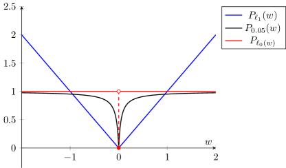
Figure 2: Different choices of penalty functions with ${n_{s}}=1$.

4.2 MM approach and reweighted $\ell_{1}$ algorithm

The idea behind the MM approach is to solve a sequence of optimization problems whose solutions converge to that of the original problem [16, 17]. This sequence is generated by a carefully constructed surrogate that satisfies two properties—the surrogate must majorize the objective function for all values, and the surrogate must match the objective function at the current iterate. More specifically, suppose

$$J({\mathchoice{\mbox{\boldmath$\displaystyle{w}$}}{\mbox{\boldmath$\textstyle{w}$}}{\mbox{\boldmath$\scriptstyle{w}$}}{\mbox{\boldmath$\scriptscriptstyle{w}$}}})=\Phi({\mathchoice{\mbox{\boldmath$\displaystyle{w}$}}{\mbox{\boldmath$\textstyle{w}$}}{\mbox{\boldmath$\scriptstyle{w}$}}{\mbox{\boldmath$\scriptscriptstyle{w}$}}})+\gamma\sum_{i=1}^{n_{s}}\frac{w_{i}}{w_{i}+\epsilon}.$$

Then the surrogate function $g({\mathchoice{\mbox{\boldmath$\displaystyle{w}$}}{\mbox{\boldmath$\textstyle{w}$}}{\mbox{\boldmath$\scriptstyle{w}$}}{\mbox{\boldmath$\scriptscriptstyle{w}$}}}|{\mathchoice{\mbox{\boldmath$\displaystyle{w}$}}{\mbox{\boldmath$\textstyle{w}$}}{\mbox{\boldmath$\scriptstyle{w}$}}{\mbox{\boldmath$\scriptscriptstyle{w}$}}}^{(m)})$ at the current iterate ${\mathchoice{\mbox{\boldmath$\displaystyle{w}$}}{\mbox{\boldmath$\textstyle{w}$}}{\mbox{\boldmath$\scriptstyle{w}$}}{\mbox{\boldmath$\scriptscriptstyle{w}$}}}^{(m)}$ must satisfy

$$g({\mathchoice{\mbox{\boldmath$\displaystyle{w}$}}{\mbox{\boldmath$\textstyle{w}$}}{\mbox{\boldmath$\scriptstyle{w}$}}{\mbox{\boldmath$\scriptscriptstyle{w}$}}}|{\mathchoice{\mbox{\boldmath$\displaystyle{w}$}}{\mbox{\boldmath$\textstyle{w}$}}{\mbox{\boldmath$\scriptstyle{w}$}}{\mbox{\boldmath$\scriptscriptstyle{w}$}}}^{(m)}) \geq J({\mathchoice{\mbox{\boldmath$\displaystyle{w}$}}{\mbox{\boldmath$\textstyle{w}$}}{\mbox{\boldmath$\scriptstyle{w}$}}{\mbox{\boldmath$\scriptscriptstyle{w}$}}})\quad\forall{\mathchoice{\mbox{\boldmath$\displaystyle{w}$}}{\mbox{\boldmath$\textstyle{w}$}}{\mbox{\boldmath$\scriptstyle{w}$}}{\mbox{\boldmath$\scriptscriptstyle{w}$}}}\in\mathcal{W},$$

$$g({\mathchoice{\mbox{\boldmath$\displaystyle{w}$}}{\mbox{\boldmath$\textstyle{w}$}}{\mbox{\boldmath$\scriptstyle{w}$}}{\mbox{\boldmath$\scriptscriptstyle{w}$}}}^{(m)}|{\mathchoice{\mbox{\boldmath$\displaystyle{w}$}}{\mbox{\boldmath$\textstyle{w}$}}{\mbox{\boldmath$\scriptstyle{w}$}}{\mbox{\boldmath$\scriptscriptstyle{w}$}}}^{(m)}) =J({\mathchoice{\mbox{\boldmath$\displaystyle{w}$}}{\mbox{\boldmath$\textstyle{w}$}}{\mbox{\boldmath$\scriptstyle{w}$}}{\mbox{\boldmath$\scriptscriptstyle{w}$}}}^{(m)}).$$

Granted the existence of this surrogate function, to find the next iterate ${\mathchoice{\mbox{\boldmath$\displaystyle{w}$}}{\mbox{\boldmath$\textstyle{w}$}}{\mbox{\boldmath$\scriptstyle{w}$}}{\mbox{\boldmath$\scriptscriptstyle{w}$}}}^{(m+1)}$ we solve the optimization problem

(22) $${\mathchoice{\mbox{\boldmath$\displaystyle{w}$}}{\mbox{\boldmath$\textstyle{w}$}}{\mbox{\boldmath$\scriptstyle{w}$}}{\mbox{\boldmath$\scriptscriptstyle{w}$}}}^{(m+1)}=\operatorname*{arg\,min}_{{\mathchoice{\mbox{\boldmath$\displaystyle{w}$}}{\mbox{\boldmath$\textstyle{w}$}}{\mbox{\boldmath$\scriptstyle{w}$}}{\mbox{\boldmath$\scriptscriptstyle{w}$}}}\in\mathcal{W}}g({\mathchoice{\mbox{\boldmath$\displaystyle{w}$}}{\mbox{\boldmath$\textstyle{w}$}}{\mbox{\boldmath$\scriptstyle{w}$}}{\mbox{\boldmath$\scriptscriptstyle{w}$}}}|{\mathchoice{\mbox{\boldmath$\displaystyle{w}$}}{\mbox{\boldmath$\textstyle{w}$}}{\mbox{\boldmath$\scriptstyle{w}$}}{\mbox{\boldmath$\scriptscriptstyle{w}$}}}^{(m)}).$$

To show the objective function decreases at the next iterate, observe that the next iterate ${\mathchoice{\mbox{\boldmath$\displaystyle{w}$}}{\mbox{\boldmath$\textstyle{w}$}}{\mbox{\boldmath$\scriptstyle{w}$}}{\mbox{\boldmath$\scriptscriptstyle{w}$}}}^{(m+1)}$ stays within the feasible region and use the two properties of the surrogate function

$$J({\mathchoice{\mbox{\boldmath$\displaystyle{w}$}}{\mbox{\boldmath$\textstyle{w}$}}{\mbox{\boldmath$\scriptstyle{w}$}}{\mbox{\boldmath$\scriptscriptstyle{w}$}}}^{(m+1)})\leq g({\mathchoice{\mbox{\boldmath$\displaystyle{w}$}}{\mbox{\boldmath$\textstyle{w}$}}{\mbox{\boldmath$\scriptstyle{w}$}}{\mbox{\boldmath$\scriptscriptstyle{w}$}}}^{(m+1)}|{\mathchoice{\mbox{\boldmath$\displaystyle{w}$}}{\mbox{\boldmath$\textstyle{w}$}}{\mbox{\boldmath$\scriptstyle{w}$}}{\mbox{\boldmath$\scriptscriptstyle{w}$}}}^{(m)})\leq g({\mathchoice{\mbox{\boldmath$\displaystyle{w}$}}{\mbox{\boldmath$\textstyle{w}$}}{\mbox{\boldmath$\scriptstyle{w}$}}{\mbox{\boldmath$\scriptscriptstyle{w}$}}}^{(m)}|{\mathchoice{\mbox{\boldmath$\displaystyle{w}$}}{\mbox{\boldmath$\textstyle{w}$}}{\mbox{\boldmath$\scriptstyle{w}$}}{\mbox{\boldmath$\scriptscriptstyle{w}$}}}^{(m)})=J({\mathchoice{\mbox{\boldmath$\displaystyle{w}$}}{\mbox{\boldmath$\textstyle{w}$}}{\mbox{\boldmath$\scriptstyle{w}$}}{\mbox{\boldmath$\scriptscriptstyle{w}$}}}^{(m)}).$$

To construct this surrogate function, we use the fact that a concave function is below its tangent [17, Equation (4.7)]. Applying this to our concave penalty $P_{\epsilon}({\mathchoice{\mbox{\boldmath$\displaystyle{w}$}}{\mbox{\boldmath$\textstyle{w}$}}{\mbox{\boldmath$\scriptstyle{w}$}}{\mbox{\boldmath$\scriptscriptstyle{w}$}}})$, we have

$$P_{\epsilon}({\mathchoice{\mbox{\boldmath$\displaystyle{w}$}}{\mbox{\boldmath$\textstyle{w}$}}{\mbox{\boldmath$\scriptstyle{w}$}}{\mbox{\boldmath$\scriptscriptstyle{w}$}}})\leq P_{\epsilon}({\mathchoice{\mbox{\boldmath$\displaystyle{w}$}}{\mbox{\boldmath$\textstyle{w}$}}{\mbox{\boldmath$\scriptstyle{w}$}}{\mbox{\boldmath$\scriptscriptstyle{w}$}}}^{(m)})+({\mathchoice{\mbox{\boldmath$\displaystyle{w}$}}{\mbox{\boldmath$\textstyle{w}$}}{\mbox{\boldmath$\scriptstyle{w}$}}{\mbox{\boldmath$\scriptscriptstyle{w}$}}}-{\mathchoice{\mbox{\boldmath$\displaystyle{w}$}}{\mbox{\boldmath$\textstyle{w}$}}{\mbox{\boldmath$\scriptstyle{w}$}}{\mbox{\boldmath$\scriptscriptstyle{w}$}}}^{(m)})^{\top}\nabla_{{\mathchoice{\mbox{\boldmath$\displaystyle{w}$}}{\mbox{\boldmath$\textstyle{w}$}}{\mbox{\boldmath$\scriptstyle{w}$}}{\mbox{\boldmath$\scriptscriptstyle{w}$}}}}P_{\epsilon}({\mathchoice{\mbox{\boldmath$\displaystyle{w}$}}{\mbox{\boldmath$\textstyle{w}$}}{\mbox{\boldmath$\scriptstyle{w}$}}{\mbox{\boldmath$\scriptscriptstyle{w}$}}}^{(m)}),\quad\text{for all }{\mathchoice{\mbox{\boldmath$\displaystyle{w}$}}{\mbox{\boldmath$\textstyle{w}$}}{\mbox{\boldmath$\scriptstyle{w}$}}{\mbox{\boldmath$\scriptscriptstyle{w}$}}}\in\mathcal{W}.$$

With this majorization relation, we define the surrogate function to be

$$g({\mathchoice{\mbox{\boldmath$\displaystyle{w}$}}{\mbox{\boldmath$\textstyle{w}$}}{\mbox{\boldmath$\scriptstyle{w}$}}{\mbox{\boldmath$\scriptscriptstyle{w}$}}}|{\mathchoice{\mbox{\boldmath$\displaystyle{w}$}}{\mbox{\boldmath$\textstyle{w}$}}{\mbox{\boldmath$\scriptstyle{w}$}}{\mbox{\boldmath$\scriptscriptstyle{w}$}}}^{(m)})=\Phi({\mathchoice{\mbox{\boldmath$\displaystyle{w}$}}{\mbox{\boldmath$\textstyle{w}$}}{\mbox{\boldmath$\scriptstyle{w}$}}{\mbox{\boldmath$\scriptscriptstyle{w}$}}})+\gamma\left(P_{\epsilon}({\mathchoice{\mbox{\boldmath$\displaystyle{w}$}}{\mbox{\boldmath$\textstyle{w}$}}{\mbox{\boldmath$\scriptstyle{w}$}}{\mbox{\boldmath$\scriptscriptstyle{w}$}}}^{(m)})+({\mathchoice{\mbox{\boldmath$\displaystyle{w}$}}{\mbox{\boldmath$\textstyle{w}$}}{\mbox{\boldmath$\scriptstyle{w}$}}{\mbox{\boldmath$\scriptscriptstyle{w}$}}}-{\mathchoice{\mbox{\boldmath$\displaystyle{w}$}}{\mbox{\boldmath$\textstyle{w}$}}{\mbox{\boldmath$\scriptstyle{w}$}}{\mbox{\boldmath$\scriptscriptstyle{w}$}}}^{(m)})^{\top}\nabla_{{\mathchoice{\mbox{\boldmath$\displaystyle{w}$}}{\mbox{\boldmath$\textstyle{w}$}}{\mbox{\boldmath$\scriptstyle{w}$}}{\mbox{\boldmath$\scriptscriptstyle{w}$}}}}P_{\epsilon}({\mathchoice{\mbox{\boldmath$\displaystyle{w}$}}{\mbox{\boldmath$\textstyle{w}$}}{\mbox{\boldmath$\scriptstyle{w}$}}{\mbox{\boldmath$\scriptscriptstyle{w}$}}}^{(m)})\right)$$

By dropping the terms that do not depend on $\textstyle{w}$, it can be readily verified that Eq. 22 can be replaced by the equivalent problem

(23) $${\mathchoice{\mbox{\boldmath$\displaystyle{w}$}}{\mbox{\boldmath$\textstyle{w}$}}{\mbox{\boldmath$\scriptstyle{w}$}}{\mbox{\boldmath$\scriptscriptstyle{w}$}}}^{(m+1)}= \>\operatorname*{arg\,min}_{{\mathchoice{\mbox{\boldmath$\displaystyle{w}$}}{\mbox{\boldmath$\textstyle{w}$}}{\mbox{\boldmath$\scriptstyle{w}$}}{\mbox{\boldmath$\scriptscriptstyle{w}$}}}\in\mathcal{W}}\Phi({\mathchoice{\mbox{\boldmath$\displaystyle{w}$}}{\mbox{\boldmath$\textstyle{w}$}}{\mbox{\boldmath$\scriptstyle{w}$}}{\mbox{\boldmath$\scriptscriptstyle{w}$}}})+\gamma\sum_{i=1}^{n_{s}}\frac{\epsilon w_{i}}{(w_{i}^{(m)}+\epsilon)^{2}}$$

$$= \>\operatorname*{arg\,min}_{{\mathchoice{\mbox{\boldmath$\displaystyle{w}$}}{\mbox{\boldmath$\textstyle{w}$}}{\mbox{\boldmath$\scriptstyle{w}$}}{\mbox{\boldmath$\scriptscriptstyle{w}$}}}\in\mathcal{W}}\Phi({\mathchoice{\mbox{\boldmath$\displaystyle{w}$}}{\mbox{\boldmath$\textstyle{w}$}}{\mbox{\boldmath$\scriptstyle{w}$}}{\mbox{\boldmath$\scriptscriptstyle{w}$}}})+\gamma\|{\mathchoice{\mbox{\boldmath$\displaystyle{R}$}}{\mbox{\boldmath$\textstyle{R}$}}{\mbox{\boldmath$\scriptstyle{R}$}}{\mbox{\boldmath$\scriptscriptstyle{R}$}}}({\mathchoice{\mbox{\boldmath$\displaystyle{w}$}}{\mbox{\boldmath$\textstyle{w}$}}{\mbox{\boldmath$\scriptstyle{w}$}}{\mbox{\boldmath$\scriptscriptstyle{w}$}}}^{(m)}){\mathchoice{\mbox{\boldmath$\displaystyle{w}$}}{\mbox{\boldmath$\textstyle{w}$}}{\mbox{\boldmath$\scriptstyle{w}$}}{\mbox{\boldmath$\scriptscriptstyle{w}$}}}\|_{1},$$

where ${\mathchoice{\mbox{\boldmath$\displaystyle{R}$}}{\mbox{\boldmath$\textstyle{R}$}}{\mbox{\boldmath$\scriptstyle{R}$}}{\mbox{\boldmath$\scriptscriptstyle{R}$}}}({\mathchoice{\mbox{\boldmath$\displaystyle{w}$}}{\mbox{\boldmath$\textstyle{w}$}}{\mbox{\boldmath$\scriptstyle{w}$}}{\mbox{\boldmath$\scriptscriptstyle{w}$}}})=\text{diag}\left(\frac{\epsilon}{(w_{1}+\epsilon)^{2}},\dots,\frac{\epsilon}{(w_{n_{s}}+\epsilon)^{2}}\right)$. We see that Eq. 23 is of the form of a reweighted $\ell_{1}$-optimization problem. The details of the optimization procedure are given in Algorithm 3. (We remark that, in Algorithm 3, other metrics measuring the difference between the successive weight vectors can be used in step 3.)

Algorithm 3 Reweighted $\ell_{1}$ Algorithm.

0:  Initial guess ${\mathchoice{\mbox{\boldmath$\displaystyle{w}$}}{\mbox{\boldmath$\textstyle{w}$}}{\mbox{\boldmath$\scriptstyle{w}$}}{\mbox{\boldmath$\scriptscriptstyle{w}$}}}^{(0)}\in\mathbb{R}^{n_{s}}$, stopping tolerance tol, penalty parameters $\gamma,\epsilon\geq 0$.

0:  Optimal design ${\mathchoice{\mbox{\boldmath$\displaystyle{w}$}}{\mbox{\boldmath$\textstyle{w}$}}{\mbox{\boldmath$\scriptstyle{w}$}}{\mbox{\boldmath$\scriptscriptstyle{w}$}}}^{*}\in\mathbb{R}^{n_{s}}$.

1:  Initialize $m=1$.

2:  Compute

$${\mathchoice{\mbox{\boldmath$\displaystyle{w}$}}{\mbox{\boldmath$\textstyle{w}$}}{\mbox{\boldmath$\scriptstyle{w}$}}{\mbox{\boldmath$\scriptscriptstyle{w}$}}}^{(1)}=\operatorname*{arg\,min}_{{\mathchoice{\mbox{\boldmath$\displaystyle{w}$}}{\mbox{\boldmath$\textstyle{w}$}}{\mbox{\boldmath$\scriptstyle{w}$}}{\mbox{\boldmath$\scriptscriptstyle{w}$}}}\in\mathcal{W}}\Phi({\mathchoice{\mbox{\boldmath$\displaystyle{w}$}}{\mbox{\boldmath$\textstyle{w}$}}{\mbox{\boldmath$\scriptstyle{w}$}}{\mbox{\boldmath$\scriptscriptstyle{w}$}}})+\gamma\|{\mathchoice{\mbox{\boldmath$\displaystyle{w}$}}{\mbox{\boldmath$\textstyle{w}$}}{\mbox{\boldmath$\scriptstyle{w}$}}{\mbox{\boldmath$\scriptscriptstyle{w}$}}}\|_{1}.$$

3:  while $m<m_{max}$ and $\|{\mathchoice{\mbox{\boldmath$\displaystyle{w}$}}{\mbox{\boldmath$\textstyle{w}$}}{\mbox{\boldmath$\scriptstyle{w}$}}{\mbox{\boldmath$\scriptscriptstyle{w}$}}}^{(m)}-{\mathchoice{\mbox{\boldmath$\displaystyle{w}$}}{\mbox{\boldmath$\textstyle{w}$}}{\mbox{\boldmath$\scriptstyle{w}$}}{\mbox{\boldmath$\scriptscriptstyle{w}$}}}^{(m-1)}\|_{2}>\text{tol}$ do

4:     Update $m=m+1$

5:     Compute

$${\mathchoice{\mbox{\boldmath$\displaystyle{w}$}}{\mbox{\boldmath$\textstyle{w}$}}{\mbox{\boldmath$\scriptstyle{w}$}}{\mbox{\boldmath$\scriptscriptstyle{w}$}}}^{(m)}=\operatorname*{arg\,min}_{{\mathchoice{\mbox{\boldmath$\displaystyle{w}$}}{\mbox{\boldmath$\textstyle{w}$}}{\mbox{\boldmath$\scriptstyle{w}$}}{\mbox{\boldmath$\scriptscriptstyle{w}$}}}\in\mathcal{W}}\Phi({\mathchoice{\mbox{\boldmath$\displaystyle{w}$}}{\mbox{\boldmath$\textstyle{w}$}}{\mbox{\boldmath$\scriptstyle{w}$}}{\mbox{\boldmath$\scriptscriptstyle{w}$}}})+\gamma\sum_{i=1}^{n_{s}}r_{i}\cdot w_{i},$$

6:     Update

$$r_{i}=\frac{\epsilon}{(|w_{i}^{(m-1)}|+\epsilon)^{2}},\quad i=1,\ldots,n_{s}.$$

7:  end while

8:  Return ${\mathchoice{\mbox{\boldmath$\displaystyle{w}$}}{\mbox{\boldmath$\textstyle{w}$}}{\mbox{\boldmath$\scriptstyle{w}$}}{\mbox{\boldmath$\scriptscriptstyle{w}$}}}^{(m)}={\mathchoice{\mbox{\boldmath$\displaystyle{w}$}}{\mbox{\boldmath$\textstyle{w}$}}{\mbox{\boldmath$\scriptstyle{w}$}}{\mbox{\boldmath$\scriptscriptstyle{w}$}}}^{*}.$

We conclude this section with a few remarks regarding this algorithm. In our application, $\Phi({\mathchoice{\mbox{\boldmath$\displaystyle{w}$}}{\mbox{\boldmath$\textstyle{w}$}}{\mbox{\boldmath$\scriptstyle{w}$}}{\mbox{\boldmath$\scriptscriptstyle{w}$}}})$ is convex; therefore, each subproblem to update the design weights is also convex. To initialize the reweighted $\ell_{1}$ algorithm, we start with the weights $r_{i}=1$, $i=1,\ldots,{n_{s}}$. This ensures that, in the first step, we are computing the solution of the $\ell_{1}$-penalized optimization problem. The subsequent reweighted $\ell_{1}$ iterations further promote binary designs. To solve the subproblems in each reweighted $\ell_{1}$ iteration we use an interior point algorithm; however, any solver for appropriate convex optimization may be used. In Section 6, we will provide a discussion of our choice of $\epsilon$ for our application. It is also worth mentioning that besides the penalty function $P_{\epsilon}$ used above, another possible choice is $\sum_{i=1}^{n_{s}}\arctan(|w_{i}|/\epsilon)$ which yields the weights $\frac{1}{|w_{i}|^{2}+\epsilon^{2}}$.

5 Modifed A-optimal criterion

Motivated by reducing the computational cost of computing A-optimal designs, in this section, we introduce a modified A-optimality criterion. As mentioned in [8], we can consider a weighted A-optimal criterion $\mathsf{tr}\,\left(\boldsymbol{\Gamma}\mathbf{\Gamma}_{\text{post}}({\mathchoice{\mbox{\boldmath$\displaystyle{w}$}}{\mbox{\boldmath$\textstyle{w}$}}{\mbox{\boldmath$\scriptstyle{w}$}}{\mbox{\boldmath$\scriptscriptstyle{w}$}}})\right)$, where $\boldsymbol{\Gamma}$ is a positive semidefinite weighting matrix. Similar to Eq. 5, we work with $\mathsf{tr}\,\left(\boldsymbol{\Gamma}(\mathbf{\Gamma}_{\text{post}}-\mathbf{\Gamma}_{\text{pr}})\right)$, since the term $\mathsf{tr}\,\left(\boldsymbol{\Gamma}(\mathbf{\Gamma}_{\text{pr}})\right)$ is independent of the weights $\textstyle{w}$. By choosing $\boldsymbol{\Gamma}=\mathbf{\Gamma}^{-1}_{\text{pr}}$, we obtain the modified A-optimal criterion

(24) $$\Phi_{\text{mod}}{({\mathchoice{\mbox{\boldmath$\displaystyle{w}$}}{\mbox{\boldmath$\textstyle{w}$}}{\mbox{\boldmath$\scriptstyle{w}$}}{\mbox{\boldmath$\scriptscriptstyle{w}$}}})}\equiv\mathsf{tr}\,\left(\left(\mathbf{I}+\mathbfcal{H}_{\text{m}}({\mathchoice{\mbox{\boldmath$\displaystyle{w}$}}{\mbox{\boldmath$\textstyle{w}$}}{\mbox{\boldmath$\scriptstyle{w}$}}{\mbox{\boldmath$\scriptscriptstyle{w}$}}})\right)^{-1}-\mathbf{I}\right).$$

Note that the expression for $\Phi_{\text{mod}}{({\mathchoice{\mbox{\boldmath$\displaystyle{w}$}}{\mbox{\boldmath$\textstyle{w}$}}{\mbox{\boldmath$\scriptstyle{w}$}}{\mbox{\boldmath$\scriptscriptstyle{w}$}}})}$ remains meaningful in the infinite-dimensional limit. This can be seen by noting that

$$\Phi_{\text{mod}}{({\mathchoice{\mbox{\boldmath$\displaystyle{w}$}}{\mbox{\boldmath$\textstyle{w}$}}{\mbox{\boldmath$\scriptstyle{w}$}}{\mbox{\boldmath$\scriptscriptstyle{w}$}}})}=\mathsf{tr}\,\left(\big{(}\mathbf{I}+\mathbfcal{H}_{\text{m}}({\mathchoice{\mbox{\boldmath$\displaystyle{w}$}}{\mbox{\boldmath$\textstyle{w}$}}{\mbox{\boldmath$\scriptstyle{w}$}}{\mbox{\boldmath$\scriptscriptstyle{w}$}}})\big{)}^{-1}-\mathbf{I}\right)=-\mathsf{tr}\,\left(\mathbfcal{H}_{\text{m}}({\mathchoice{\mbox{\boldmath$\displaystyle{w}$}}{\mbox{\boldmath$\textstyle{w}$}}{\mbox{\boldmath$\scriptstyle{w}$}}{\mbox{\boldmath$\scriptscriptstyle{w}$}}})\big{(}\mathbf{I}+\mathbfcal{H}_{\text{m}}({\mathchoice{\mbox{\boldmath$\displaystyle{w}$}}{\mbox{\boldmath$\textstyle{w}$}}{\mbox{\boldmath$\scriptstyle{w}$}}{\mbox{\boldmath$\scriptscriptstyle{w}$}}})\big{)}^{-1}\right),$$

and using the fact that in the infinite-dimensional limit, for every ${\mathchoice{\mbox{\boldmath$\displaystyle{w}$}}{\mbox{\boldmath$\textstyle{w}$}}{\mbox{\boldmath$\scriptstyle{w}$}}{\mbox{\boldmath$\scriptscriptstyle{w}$}}}\in[0,1]^{n_{s}}$, $\mathbfcal{H}_{\text{m}}({\mathchoice{\mbox{\boldmath$\displaystyle{w}$}}{\mbox{\boldmath$\textstyle{w}$}}{\mbox{\boldmath$\scriptstyle{w}$}}{\mbox{\boldmath$\scriptscriptstyle{w}$}}})$ is trace class and $\big{(}\mathbf{I}+\mathbfcal{H}_{\text{m}}({\mathchoice{\mbox{\boldmath$\displaystyle{w}$}}{\mbox{\boldmath$\textstyle{w}$}}{\mbox{\boldmath$\scriptstyle{w}$}}{\mbox{\boldmath$\scriptscriptstyle{w}$}}})\big{)}^{-1}$ is a bounded linear operator.

We show in our numerical results that the modified A-optimality criterion can be useful in practice, if a cheaper alternative to the A-optimal criterion is desired, and minimizing $\Phi_{\text{mod}}{}$ can provide designs that lead to small posterior uncertainty.

5.1 Derivation of estimators

Here we seek to improve the efficiency of the modified A-optimal criterion by computing a randomized estimator for the modified A-optimal criterion and its gradient. As in the previous derivation of our estimators, we replace $\mathbfcal{H}_{\text{m}}({\mathchoice{\mbox{\boldmath$\displaystyle{w}$}}{\mbox{\boldmath$\textstyle{w}$}}{\mbox{\boldmath$\scriptstyle{w}$}}{\mbox{\boldmath$\scriptscriptstyle{w}$}}})$ by its low rank approximation to obtain the randomized estimator for the modified A-optimal criterion

(25) $$\Phi_{\text{mod}}{({\mathchoice{\mbox{\boldmath$\displaystyle{w}$}}{\mbox{\boldmath$\textstyle{w}$}}{\mbox{\boldmath$\scriptstyle{w}$}}{\mbox{\boldmath$\scriptscriptstyle{w}$}}})}\approx\mathsf{tr}\,\left((\mathbf{I}+\widehat{\mathbfcal{H}}_{\text{m}}({\mathchoice{\mbox{\boldmath$\displaystyle{w}$}}{\mbox{\boldmath$\textstyle{w}$}}{\mbox{\boldmath$\scriptstyle{w}$}}{\mbox{\boldmath$\scriptscriptstyle{w}$}}}))^{-1}-\mathbf{I}\right)\equiv\widehat{\Phi}_{\text{mod}}{({\mathchoice{\mbox{\boldmath$\displaystyle{w}$}}{\mbox{\boldmath$\textstyle{w}$}}{\mbox{\boldmath$\scriptstyle{w}$}}{\mbox{\boldmath$\scriptscriptstyle{w}$}}};\ell)}.$$

Similarly, we use the same low-rank approximation ${\widehat{\mathbfcal{H}}_{\text{m}}}({\mathchoice{\mbox{\boldmath$\displaystyle{w}$}}{\mbox{\boldmath$\textstyle{w}$}}{\mbox{\boldmath$\scriptstyle{w}$}}{\mbox{\boldmath$\scriptscriptstyle{w}$}}})$ in the gradient of the modified A-optimal criterion to obtain the randomized estimator

(26) $$\widehat{\partial_{j}\Phi}_{\text{mod}}({\mathchoice{\mbox{\boldmath$\displaystyle{w}$}}{\mbox{\boldmath$\textstyle{w}$}}{\mbox{\boldmath$\scriptstyle{w}$}}{\mbox{\boldmath$\scriptscriptstyle{w}$}}};\ell)=-\mathsf{tr}\,\left((\mathbf{I}+{\widehat{\mathbfcal{H}}_{\text{m}}}({\mathchoice{\mbox{\boldmath$\displaystyle{w}$}}{\mbox{\boldmath$\textstyle{w}$}}{\mbox{\boldmath$\scriptstyle{w}$}}{\mbox{\boldmath$\scriptscriptstyle{w}$}}}))^{-1}{\mathbfcal{F}}^{T}\mathbf{E}_{j}^{\text{noise}}{\mathbfcal{F}}(\mathbf{I}+{\widehat{\mathbfcal{H}}_{\text{m}}}({\mathchoice{\mbox{\boldmath$\displaystyle{w}$}}{\mbox{\boldmath$\textstyle{w}$}}{\mbox{\boldmath$\scriptstyle{w}$}}{\mbox{\boldmath$\scriptscriptstyle{w}$}}}))^{-1}\right),$$

for $j=1,\dots,n_{s}$.

5.2 Computational procedure and cost

Using similar techniques as those described in Section 3.1, we can write the estimator for the modified A-optimal criterion in terms of the eigenvalues of $\mathbf{T}$:

(27) $$\widehat{\Phi}_{\text{mod}}{({\mathchoice{\mbox{\boldmath$\displaystyle{w}$}}{\mbox{\boldmath$\textstyle{w}$}}{\mbox{\boldmath$\scriptstyle{w}$}}{\mbox{\boldmath$\scriptscriptstyle{w}$}}};\ell)}=-\mathsf{tr}\,\left(\mathbf{D}_{\mathbf{T}}\right).$$

Moreover,

(28) $$\widehat{\partial_{j}\Phi}_{\text{mod}}({\mathchoice{\mbox{\boldmath$\displaystyle{w}$}}{\mbox{\boldmath$\textstyle{w}$}}{\mbox{\boldmath$\scriptstyle{w}$}}{\mbox{\boldmath$\scriptscriptstyle{w}$}}}) =-\mathsf{tr}\,\left({\mathbfcal{F}}^{\top}\mathbf{E}_{j}^{\text{noise}}{\mathbfcal{F}}\right)+2\mathsf{tr}\,\left({\mathbfcal{F}}\mathbf{V}\mathbf{D}_{\mathbf{T}}\mathbf{V}^{\top}{\mathbfcal{F}}^{\top}\mathbf{E}_{j}^{\text{noise}}\right)-$$

$$\quad\mathsf{tr}\,\left({\mathbfcal{F}}\mathbf{V}\mathbf{D}_{\mathbf{T}}^{2}\mathbf{V}^{\top}{\mathbfcal{F}}^{\top}\mathbf{E}_{j}^{\text{noise}}\right).$$

with $\mathbf{D}_{\mathbf{T}}=\mathbf{\Lambda}_{\mathbf{T}}(\mathbf{I}+\mathbf{\Lambda}_{\mathbf{T}})^{-1}$ and $\mathbf{V}$ defined as in Section 3.1.

The procedure for computing the estimators for the modified A-optimal criterion follows the steps in Algorithm 2 closely. Instead of presenting an additional algorithm, we provide an overview of the computation of the estimators for the modified A-optimal criterion along with the associated computational cost in terms of the number of PDE solves.

To evaluate the estimators for the modified A-optimal criterion, the only precomputation we perform is to obtain

$$s_{j}=-\mathsf{tr}\,\left({\mathbfcal{F}}^{\top}\mathbf{E}_{j}^{\text{noise}}{\mathbfcal{F}}\right),\quad j=1,\ldots,{n_{s}}.$$

This term appears in the estimator for the gradient and accumulates a total cost of $n_{s}n_{t}$ PDE solves. The remaining terms in the estimators depend on a design $\textstyle{w}$ and, in particular, the eigenvalues and eigenvectors of ${\widehat{\mathbfcal{H}}_{\text{m}}}({\mathchoice{\mbox{\boldmath$\displaystyle{w}$}}{\mbox{\boldmath$\textstyle{w}$}}{\mbox{\boldmath$\scriptstyle{w}$}}{\mbox{\boldmath$\scriptscriptstyle{w}$}}})$. As with the estimators for the A-optimal criterion, the eigenvalues and eigenvectors of $\widehat{\mathbfcal{H}}_{\text{m}}({\mathchoice{\mbox{\boldmath$\displaystyle{w}$}}{\mbox{\boldmath$\textstyle{w}$}}{\mbox{\boldmath$\scriptstyle{w}$}}{\mbox{\boldmath$\scriptscriptstyle{w}$}}})$ are obtained by Algorithm 1. Recall that the cost associated with Algorithm 1, with $q=1$, is $4\ell$ PDE solves. Once the eigenvalues and eigenvectors are computed, Eq. 25 can be evaluated without any additional PDE solves. The remaining computational effort occurs in the evaluation of the gradient. Because of our modification to the A-optimal criterion, the expression Eq. 28 is efficiently evaluated by computing ${\mathbfcal{F}}\mathbf{V}$. Therefore, the total cost of evaluating the estimators for the modified A-optimal criterion and its gradient is $5\ell$ PDE solves. From this computational cost analysis, we see the modified A-optimal estimators require $\ell$ less PDE solves than the A-optimal estimators.

5.3 Error analysis

We now quantify the absolute error of our estimators with the following theorem.

Theorem 5.1.

Let $\widehat{\Phi}_{\text{mod}}{({\mathchoice{\mbox{\boldmath$\displaystyle{w}$}}{\mbox{\boldmath$\textstyle{w}$}}{\mbox{\boldmath$\scriptstyle{w}$}}{\mbox{\boldmath$\scriptscriptstyle{w}$}}};\ell)}$ and $\widehat{\nabla\Phi}_{\text{mod}}({\mathchoice{\mbox{\boldmath$\displaystyle{w}$}}{\mbox{\boldmath$\textstyle{w}$}}{\mbox{\boldmath$\scriptstyle{w}$}}{\mbox{\boldmath$\scriptscriptstyle{w}$}}};\ell)$ be the randomized estimators approximating the modified A-optimal objective function $\Phi_{\text{mod}}{({\mathchoice{\mbox{\boldmath$\displaystyle{w}$}}{\mbox{\boldmath$\textstyle{w}$}}{\mbox{\boldmath$\scriptstyle{w}$}}{\mbox{\boldmath$\scriptscriptstyle{w}$}}})}$ and its gradient $\nabla\Phi_{\text{mod}}{({\mathchoice{\mbox{\boldmath$\displaystyle{w}$}}{\mbox{\boldmath$\textstyle{w}$}}{\mbox{\boldmath$\scriptstyle{w}$}}{\mbox{\boldmath$\scriptscriptstyle{w}$}}})}$, respectively. Using the notation and assumptions of Theorem 3.1, for fixed ${\mathchoice{\mbox{\boldmath$\displaystyle{w}$}}{\mbox{\boldmath$\textstyle{w}$}}{\mbox{\boldmath$\scriptstyle{w}$}}{\mbox{\boldmath$\scriptscriptstyle{w}$}}}\in[0,1]^{n_{s}}$

$$\mathbb{E}\left[|\Phi_{\text{mod}}{({\mathchoice{\mbox{\boldmath$\displaystyle{w}$}}{\mbox{\boldmath$\textstyle{w}$}}{\mbox{\boldmath$\scriptstyle{w}$}}{\mbox{\boldmath$\scriptscriptstyle{w}$}}})}-\widehat{\Phi}_{\text{mod}}{({\mathchoice{\mbox{\boldmath$\displaystyle{w}$}}{\mbox{\boldmath$\textstyle{w}$}}{\mbox{\boldmath$\scriptstyle{w}$}}{\mbox{\boldmath$\scriptscriptstyle{w}$}}};\ell)}|\right]\leq\mathsf{tr}\,\left(f(\mathbf{\Lambda}_{2})\right)+\mathsf{tr}\,\left(f(\gamma_{k}^{2q-1}C\mathbf{\Lambda}_{2})\right),$$

and for $j=1,\dots,n_{s}$,

$$\mathbb{E}\left[|\partial_{j}\Phi_{\text{mod}}{({\mathchoice{\mbox{\boldmath$\displaystyle{w}$}}{\mbox{\boldmath$\textstyle{w}$}}{\mbox{\boldmath$\scriptstyle{w}$}}{\mbox{\boldmath$\scriptscriptstyle{w}$}}})}-\widehat{\partial_{j}\Phi}_{\text{mod}}({\mathchoice{\mbox{\boldmath$\displaystyle{w}$}}{\mbox{\boldmath$\textstyle{w}$}}{\mbox{\boldmath$\scriptstyle{w}$}}{\mbox{\boldmath$\scriptscriptstyle{w}$}}};\ell)|\right]\leq 2\|\mathbf{P}_{j}\|_{2}\left(\mathsf{tr}\,\left(f(\mathbf{\Lambda}_{2})\right)+\mathsf{tr}\,\left(f(\gamma_{k}^{2q-1}C\mathbf{\Lambda}_{2})\right)\right),$$

where $C$ is defined in Eq. 16.

Proof 5.2.

See Appendix A.3.

Notice the bounds presented in Theorem 3.1 and 5.1 differ by a factor of $\|\mathbf{Z}\|_{2}$. Since the modified A-optimal criterion removes one application of $\mathbf{\Gamma}_{\text{pr}}$ from the computation of the A-optimal criterion, the bounds related to the modified A-optimal criterion no longer have the factor of $\|\mathbf{Z}\|_{2}$.

6 Numerical results

In this section, we present numerical results that test various aspects of the proposed methods. We begin by a brief description of the inverse advection-diffusion problem used to illustrate the proposed OED methods, in Section 6.1. The setup of our model problem is adapted from that in [2], where further details about the forward and inverse problem can be found. In Section 6.1, we also describle the numerical methods used for solving the forward problem, as well as the optimization solver for the OED problem. In Section 6.2, we test the accuracy of our randomized estimators and illustrate our error bounds. Then in Section 6.3, we investigate the performance of our proposed reweighted $\ell_{1}$-optimization approach. Next, we utilize the proposed optimization framework to compute A-optimal designs in Section 6.4. Finally, in Section 6.5, we compare A-optimal sensor placements with those computed by minimizing the modified A-optimal criterion.

6.1 Model problem and solvers

We consider a two-dimensional time-dependent advection-diffusion equation

$$u_{t}-\kappa\Delta u+{\mathchoice{\mbox{\boldmath$\displaystyle{v}$}}{\mbox{\boldmath$\textstyle{v}$}}{\mbox{\boldmath$\scriptstyle{v}$}}{\mbox{\boldmath$\scriptscriptstyle{v}$}}}\cdot\nabla u=0 \hskip 56.9055pt\text{in }\mathcal{D}\times(0,T),$$

$$u(\cdot,0)=m \hskip 56.9055pt\text{in }\mathcal{D},$$

$$\kappa\nabla u\cdot{\mathchoice{\mbox{\boldmath$\displaystyle{n}$}}{\mbox{\boldmath$\textstyle{n}$}}{\mbox{\boldmath$\scriptstyle{n}$}}{\mbox{\boldmath$\scriptscriptstyle{n}$}}}=0 \hskip 56.9055pt\text{on }\partial\mathcal{D}\times(0,T),$$

which models the transport of contaminants (e.g., in the atmosphere or the subsurface). Here $\kappa$ is the diffusion coefficient and is taken to be $\kappa=0.01$. The velocity field $\textstyle{v}$ is computed by solving a steady-state Navier-Stokes equations, as in [2]. The domain $\mathcal{D}$, depicted in Fig. 3, is the unit square in $\mathbb{R}^{2}$ with the gray rectangles, modeling obstacles/buildings, removed. The boundary $\partial\mathcal{D}$ is the union of the outer boundary and the boundaries of the obstacles. The PDE is discretized using linear triangular continuous Galerkin finite elements in space and implicit Euler in time. We let the final simulation time be $T=5$.

The inverse problem involves reconstructing the initial state $m$ from space-time point measurements of $u({\mathchoice{\mbox{\boldmath$\displaystyle{x}$}}{\mbox{\boldmath$\textstyle{x}$}}{\mbox{\boldmath$\scriptstyle{x}$}}{\mbox{\boldmath$\scriptscriptstyle{x}$}}},t)$. We consider ${n_{s}}=109$ sensor candidate locations distributed throughout the domain which are indicated by hollow squares in Fig. 3. Measurement data is collected from a subset of these locations at three observation times—$t=1,2,$ and $3.5$. To simulate noisy observations, 2% noise is added to the simulated data.

Recall, in Section 2, we define our prior covariance operator to be a Laplacian-like operator. Following [2], an application of the square root of the prior on $s\in L^{2}(\mathcal{D})$ is $v=\mathcal{A}^{-1}s$, which satisfies the following weak form

(29) $$\int_{\mathcal{D}}\theta\nabla v\cdot\nabla p+\alpha vp\,d{\mathchoice{\mbox{\boldmath$\displaystyle{x}$}}{\mbox{\boldmath$\textstyle{x}$}}{\mbox{\boldmath$\scriptstyle{x}$}}{\mbox{\boldmath$\scriptscriptstyle{x}$}}}=\int_{\mathcal{D}}sp\,d{\mathchoice{\mbox{\boldmath$\displaystyle{x}$}}{\mbox{\boldmath$\textstyle{x}$}}{\mbox{\boldmath$\scriptstyle{x}$}}{\mbox{\boldmath$\scriptscriptstyle{x}$}}}\qquad\text{for every }p\in H^{1}(\mathcal{D}).$$

Here $\theta$ and $\alpha$ control the variance and correlation length and are chosen to be $\alpha=0.1$ and $\theta=0.002$, respectively.

The optimization solver used for the OED problem is a quasi-Newton interior point method. Specifically, to solve each subproblem of Algorithm 3, we use MATLAB’s interior point solver provided by the fmincon function; BFGS approximation to the Hessian is used for line search. We use a vector of all ones, ${\mathchoice{\mbox{\boldmath$\displaystyle{1}$}}{\mbox{\boldmath$\textstyle{1}$}}{\mbox{\boldmath$\scriptstyle{1}$}}{\mbox{\boldmath$\scriptscriptstyle{1}$}}}\in\mathbb{R}^{n_{s}}$, as the initial guess for the optimization solver.

Figure 3: Domain with 109 candidate sensor locations.

For the numerical experiments presented in this section, the random matrix $\boldsymbol{\Omega}$ in Algorithm 1 is fixed during the optimization process. However, because of the randomness, the accuracy of the estimators, and the optimal design thus obtained, may vary with different realizations of $\boldsymbol{\Omega}$. By conducting additional numerical experiments (not reported here) the stochastic nature of the estimators resulted in minor variability (at most one or two sensor locations) in the optimal experimental designs for a modest value of $\ell$. On the other hand, if $\ell$ is sufficiently large, we observed that the same design was obtained with different realizations of $\boldsymbol{\Omega}$

6.2 Accuracy of estimators

Here we examine the accuracy of the randomized estimators with respect to $\ell$, the number of columns in the sampling matrix $\boldsymbol{\Omega}$ in the randomized subspace iteration algorithm. Specifically, we compute

$$e_{1}(\ell)=\frac{|\Phi_{\text{aopt}}{(}{\mathchoice{\mbox{\boldmath$\displaystyle{w}$}}{\mbox{\boldmath$\textstyle{w}$}}{\mbox{\boldmath$\scriptstyle{w}$}}{\mbox{\boldmath$\scriptscriptstyle{w}$}}})-\widehat{\Phi}_{\text{aopt}}{(}{\mathchoice{\mbox{\boldmath$\displaystyle{w}$}}{\mbox{\boldmath$\textstyle{w}$}}{\mbox{\boldmath$\scriptstyle{w}$}}{\mbox{\boldmath$\scriptscriptstyle{w}$}}};\ell)|}{|\Phi_{\text{aopt}}{(}{\mathchoice{\mbox{\boldmath$\displaystyle{w}$}}{\mbox{\boldmath$\textstyle{w}$}}{\mbox{\boldmath$\scriptstyle{w}$}}{\mbox{\boldmath$\scriptscriptstyle{w}$}}})|}, e_{2}(\ell)=\frac{\|\nabla\Phi_{\text{aopt}}{(}{\mathchoice{\mbox{\boldmath$\displaystyle{w}$}}{\mbox{\boldmath$\textstyle{w}$}}{\mbox{\boldmath$\scriptstyle{w}$}}{\mbox{\boldmath$\scriptscriptstyle{w}$}}})-\widehat{\nabla\Phi}_{\text{aopt}}({\mathchoice{\mbox{\boldmath$\displaystyle{w}$}}{\mbox{\boldmath$\textstyle{w}$}}{\mbox{\boldmath$\scriptstyle{w}$}}{\mbox{\boldmath$\scriptscriptstyle{w}$}}};\ell)\|_{2}}{\|\nabla\Phi_{\text{aopt}}{(}{\mathchoice{\mbox{\boldmath$\displaystyle{w}$}}{\mbox{\boldmath$\textstyle{w}$}}{\mbox{\boldmath$\scriptstyle{w}$}}{\mbox{\boldmath$\scriptscriptstyle{w}$}}})\|_{2}},$$

$$e_{3}(\ell)=\frac{|\Phi_{\text{mod}}{(}{\mathchoice{\mbox{\boldmath$\displaystyle{w}$}}{\mbox{\boldmath$\textstyle{w}$}}{\mbox{\boldmath$\scriptstyle{w}$}}{\mbox{\boldmath$\scriptscriptstyle{w}$}}})-\widehat{\Phi}_{\text{mod}}{(}{\mathchoice{\mbox{\boldmath$\displaystyle{w}$}}{\mbox{\boldmath$\textstyle{w}$}}{\mbox{\boldmath$\scriptstyle{w}$}}{\mbox{\boldmath$\scriptscriptstyle{w}$}}};\ell)|}{|\Phi_{\text{mod}}{(}{\mathchoice{\mbox{\boldmath$\displaystyle{w}$}}{\mbox{\boldmath$\textstyle{w}$}}{\mbox{\boldmath$\scriptstyle{w}$}}{\mbox{\boldmath$\scriptscriptstyle{w}$}}})|}, e_{4}(\ell)=\frac{\|\nabla\Phi_{\text{mod}}{(}{\mathchoice{\mbox{\boldmath$\displaystyle{w}$}}{\mbox{\boldmath$\textstyle{w}$}}{\mbox{\boldmath$\scriptstyle{w}$}}{\mbox{\boldmath$\scriptscriptstyle{w}$}}})-\widehat{\nabla\Phi}_{\text{mod}}({\mathchoice{\mbox{\boldmath$\displaystyle{w}$}}{\mbox{\boldmath$\textstyle{w}$}}{\mbox{\boldmath$\scriptstyle{w}$}}{\mbox{\boldmath$\scriptscriptstyle{w}$}}};\ell)\|_{2}}{\|\nabla\Phi_{\text{mod}}{(}{\mathchoice{\mbox{\boldmath$\displaystyle{w}$}}{\mbox{\boldmath$\textstyle{w}$}}{\mbox{\boldmath$\scriptstyle{w}$}}{\mbox{\boldmath$\scriptscriptstyle{w}$}}})\|_{2}},$$

with $\textstyle{w}$ taken to be a vector of all ones; that is, with all sensors activated. We let $\ell$ to vary from $17$ to $327$, because the rank of $\mathbfcal{H}_{\text{m}}({\mathchoice{\mbox{\boldmath$\displaystyle{w}$}}{\mbox{\boldmath$\textstyle{w}$}}{\mbox{\boldmath$\scriptstyle{w}$}}{\mbox{\boldmath$\scriptscriptstyle{w}$}}})$ is no larger than the number of observations taken, $n_{s}n_{t}=327$. Fig. 4 illustrates the relative error in the estimators for the A-optimal criterion and its gradient (left) and the modified A-optimal criterion and its gradient (right), as $\ell$ is varied. We observe that the error decreases rapidly with increasing $\ell$. This illustrates accuracy and efficiency of our estimators.

Next, we consider the absolute error in the estimators for the objective function and compare them with the theoretical bounds derived in Theorems 3.1 and 5.1. In Fig. 5, we compare the absolute error in the estimators with bounds from Theorem 3.1 and Theorem 5.1. As before, we take ${\mathchoice{\mbox{\boldmath$\displaystyle{w}$}}{\mbox{\boldmath$\textstyle{w}$}}{\mbox{\boldmath$\scriptstyle{w}$}}{\mbox{\boldmath$\scriptscriptstyle{w}$}}}=[1,1,\dots,1]^{\top}\in\mathbb{R}^{n_{s}}$. We observe that our error bound captures the general trend in the error. Moreover, the error bound for the modified A-optimality is better since it does not have the additional factor of $\|\mathbf{Z}\|_{2}$.

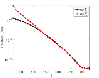
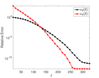
Figure 4: Relative error of the randomized estimators for the A-optimal criterion (left), and those corresponding to the modified A-optimal criterion (right) for varying $\ell$.

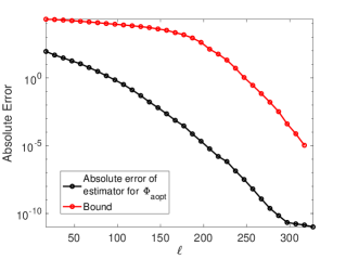
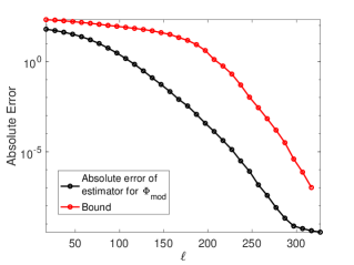
Figure 5: Absolute error bound for $\widehat{\Phi}_{\text{aopt}}({\mathchoice{\mbox{\boldmath$\displaystyle{w}$}}{\mbox{\boldmath$\textstyle{w}$}}{\mbox{\boldmath$\scriptstyle{w}$}}{\mbox{\boldmath$\scriptscriptstyle{w}$}}})$ from Theorem 3.1 (left), and $\widehat{\Phi}_{\text{mod}}({\mathchoice{\mbox{\boldmath$\displaystyle{w}$}}{\mbox{\boldmath$\textstyle{w}$}}{\mbox{\boldmath$\scriptstyle{w}$}}{\mbox{\boldmath$\scriptscriptstyle{w}$}}})$ from Theorem 5.1 (right) for varying $\ell$.

6.3 Performance of the reweighted $\ell_{1}$ algorithm

We now consider solving Eq. 10 with Algorithm 2 and 3. We first consider the choice of the value of $\epsilon$ in Eq. 23. The user-defined parameter $\epsilon$ controls the steepness of the penalty function at the origin; see Fig. 2. However, we observed that if the penalty function is too steep, the optimization solvers took more iterations without substantially altering the optimal designs. We found $\epsilon=1/2^{8}$ to be sufficiently small in our numerical experiments, and we keep this fixed for the remainder of the numerical experiments.

We perform two numerical experiments examining the impact of changing $\ell$ and the penalty parameter $\gamma$ (in Eq. 10). In the first experiment, we fix the penalty coefficient at an experimentally determined value of $\gamma=3$, and vary $\ell$; the results are recorded in Table 2. Notice when $\ell\geq 127$, the objective function value evaluated with the optimal solution, the number of active sensors, and number of subproblem solves do not change. This suggests that the randomized estimators are sufficiently accurate with $\ell=127$ and this yields a substantial reduction in computational cost.

$\ell$	subproblem solves	function count	function value	$ns_{\text{active}}$
57	10	395	39.0176	38
67	9	610	44.7219	30
77	9	790	44.5484	29
87	9	756	44.1142	30
127	9	1015	44.1139	30
207	9	978	44.1139	30
307	9	970	44.1139	30

Table 2: Number of subproblem solves Eq. 23, function evaluations, and active sensors for varying $\ell$ with the reweighted $\ell_{1}$ algorithm and $n_{s}=109$.

The second experiment involves varying $\gamma$, which indirectly controls the number of sensors in computed designs, with $\ell$ kept fixed. Here we fix $\ell=207$, which corresponds to an accuracy on the order of $10^{-7}$ for the A-optimal criterion (cf. Fig. 4). In Fig. 6, we report the design weights sorted in descending order, as $\gamma$ varies. This shows that the reweighted $\ell_{1}$ algorithm indeed produces binary designs for a range of penalty parameters. We also notice in Fig. 7 that as $\gamma$ increases the sparsity increases (i.e., the number of active sensors $ns_{\text{active}}$ decreases) and the number of function evaluations increases. The right panel compares the cost of solving an $\ell_{1}$-penalized problem for the corresponding penalty parameter $\gamma$. Since this problem is the first iterate of the reweighted $\ell_{1}$ algorithm we see that an additional cost is required to obtain binary designs and this cost increases with increasing $\gamma$ (i.e., more sparse designs).

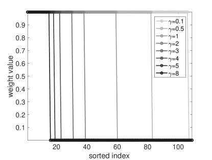
Figure 6: Optimal designs as a result of varying $\gamma$ with the reweighted $\ell_{1}$ algorithm for the A-optimal criterion. We set $\ell=207$.

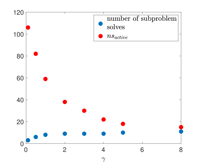
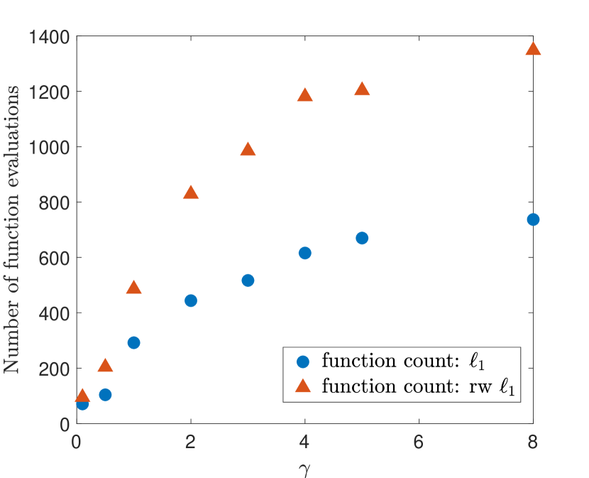
Figure 7: The effect of varying $\gamma$ on the reweighted $\ell_{1}$ algorithm for the A-optimal criterion. We set $\ell=207$.

6.4 Computing optimal designs

In Fig. 8 (left), we report an A-optimal sensor placement obtained using our optimization framework, with $\ell=207$ and $\gamma=5$; the resulting optimal sensor locations, with $18$ active sensors, are superimposed on the posterior standard deviation field. While the design is computed to yield a minimal average variance of the posterior distribution, it is also important to consider the mean of this distribution. For completeness, in Fig. 8 we show the “true“ initial condition (middle panel), used to generate synthetic data, and the mean of the resulting posterior distribution for the $18$ active sensor design (right panel).

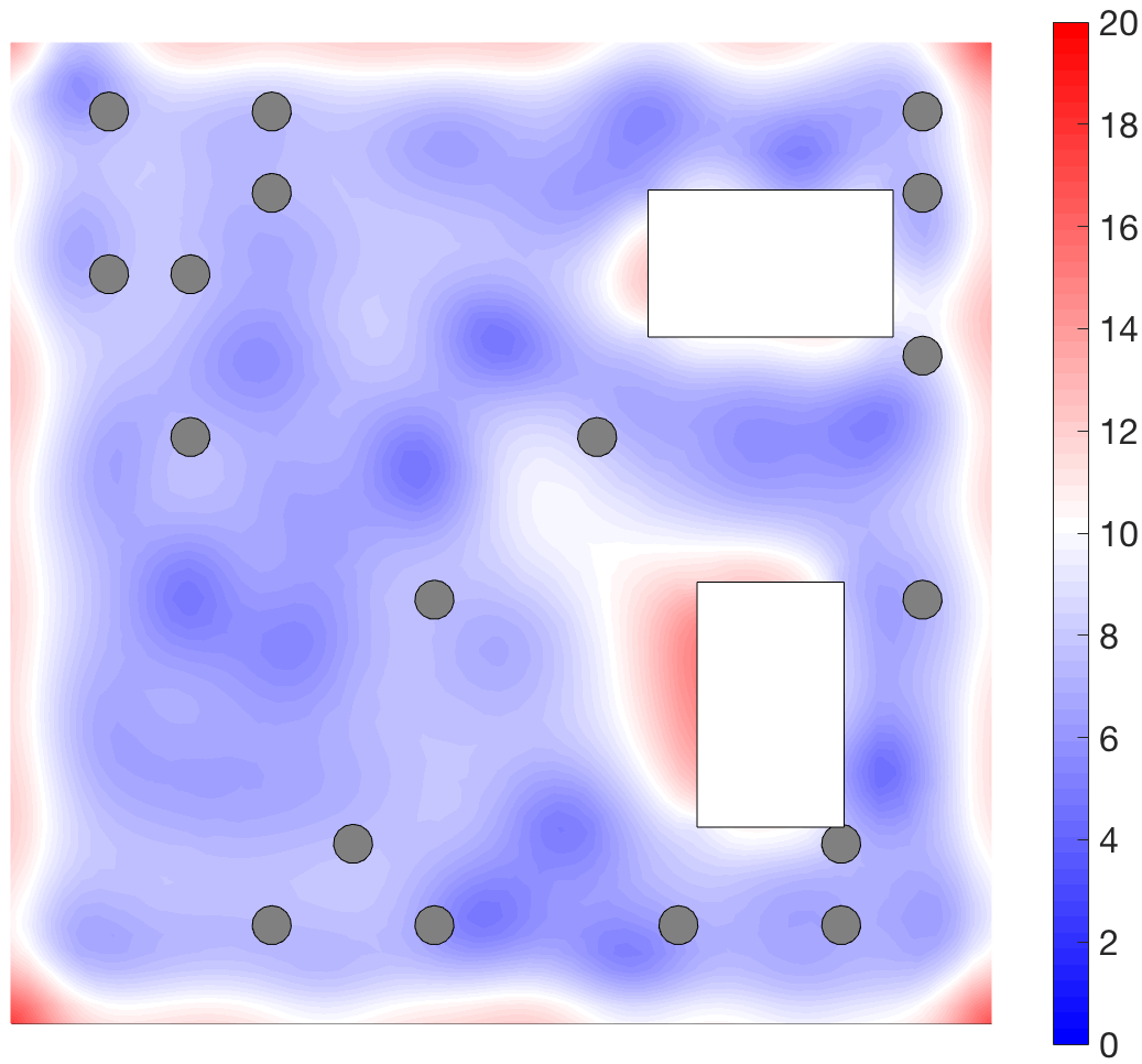
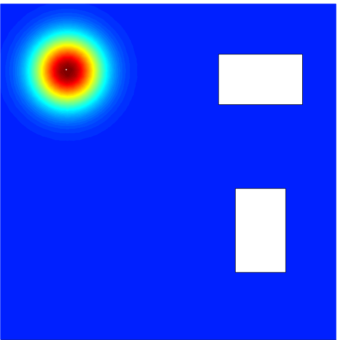
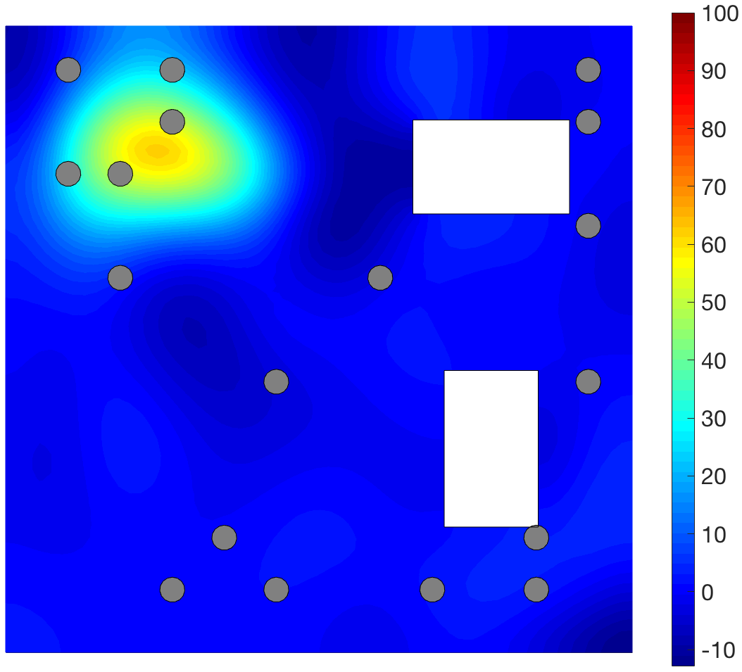
Figure 8: Standard deviation computed using the optimal design indicated by the gray circles (left). True initial condition (middle) and initial condition reconstruction (right). The optimal design was computed using $\ell=207$, the reweighted $\ell_{1}$ algorithm, and $\gamma=5$.

With the $18$ sensor design, we also illustrate the resulting uncertainty reduction by looking at the prior and posterior standard deviation fields; see Fig. 9.

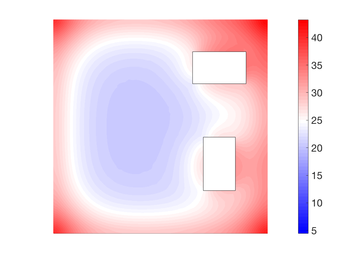
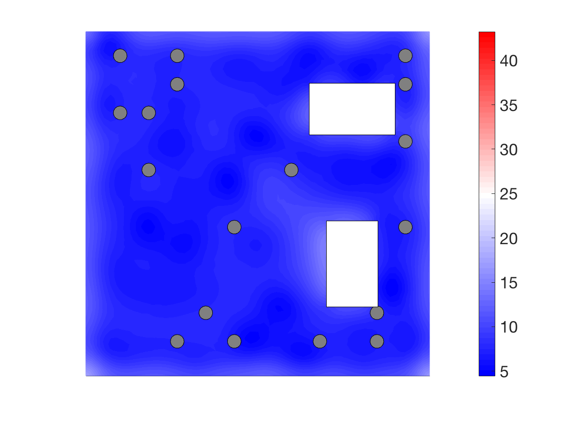
Figure 9: Comparison of the prior standard deviation field (left) with the posterior standard deviation field (right) computed using the optimal design indicated by the gray circles.

We now compare the designs obtained using the reweighted $\ell_{1}$ algorithm and our estimators against designs chosen at random, illustrating the effectiveness of the proposed A-optimal design strategy. Recall that varying $\gamma$ allows us to obtain optimal designs with different numbers of active sensors. For each value of $\gamma$, we use Algorithm 2 and 3 to compute an optimal design. We then draw $15$ random designs with the same number of active sensors as the optimal design obtained using our algorithms. To enable a consistent comparison, we evaluate the exact A-optimal criterion $\Phi_{\text{aopt}}({\mathchoice{\mbox{\boldmath$\displaystyle{w}$}}{\mbox{\boldmath$\textstyle{w}$}}{\mbox{\boldmath$\scriptstyle{w}$}}{\mbox{\boldmath$\scriptscriptstyle{w}$}}})$ at the computed optimal designs and the random ones; the results are reported in the left panel of Fig. 10. The values corresponding to the computed optimal designs are indicated as dots on the black solid line. The values obtained from the random designs are indicated by the squares. We note that the designs computed with the reweighted $\ell_{1}$ algorithm consistently beat the random designs, as expected. This observation is emphasized in the right panel of Fig. 10. Here, we compared the computed optimal design (when $\gamma=3$) with 1500 randomly generated designs using the exact trace of the posterior covariance. Again, the computed design results in a lower true A-optimal value than the random designs.

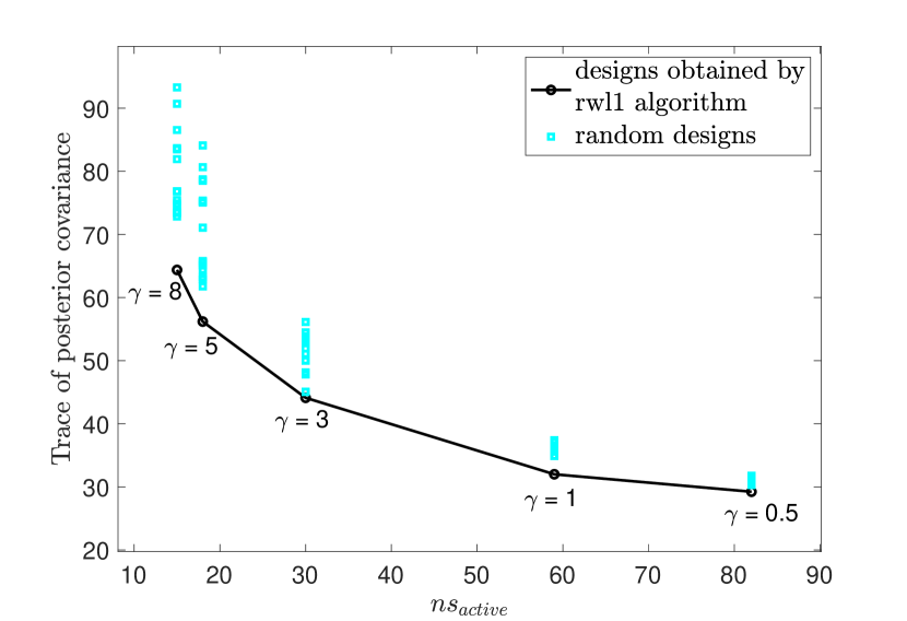
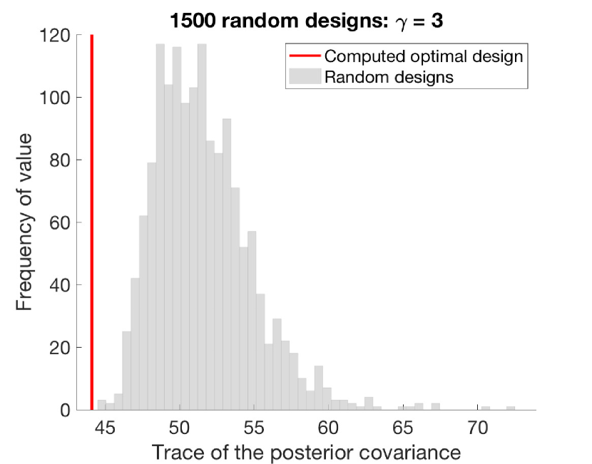
Figure 10: The true A-optimal criterion computed using the optimal and randomly generated designs. The optimal designs were computed using the A-optimal criterion and the reweighted $\ell_{1}$ algorithm for different values of $\gamma$ (left). Comparing the computed optimal design when $\gamma=3$ to 1500 randomly generated designs (right).

6.5 Comparing A-optimal and modified A-optimal designs

Here we provide a quantitative comparison of sensor placements obtained by minimizing A-optimal and modified A-optimal criteria using our proposed algorithms. Specifically, for various values of $\gamma$, we solve Eq. 10 with both the A-optimal and modified A-optimal estimators to obtain two sets of designs. By varying $\gamma$, the resulting designs obtained with the A-optimal and modified A-optimal estimators have different number of active sensors. Using both sets of designs, we evaluate the exact A-optimal criterion $\Phi_{\text{aopt}}({\mathchoice{\mbox{\boldmath$\displaystyle{w}$}}{\mbox{\boldmath$\textstyle{w}$}}{\mbox{\boldmath$\scriptstyle{w}$}}{\mbox{\boldmath$\scriptscriptstyle{w}$}}})$; these are displayed in Fig. 11. Observe that in all cases the computed A-optimal and modified A-optimal designs lead to similar levels of average posterior variance. This suggests that the modified A-optimal criterion could be used as a surrogate for the A-optimal criterion. Using the modified A-optimal criterion decreases the overall number of PDE solves and yields designs that result in values of the average posterior variance close to those produced by A-optimal designs.

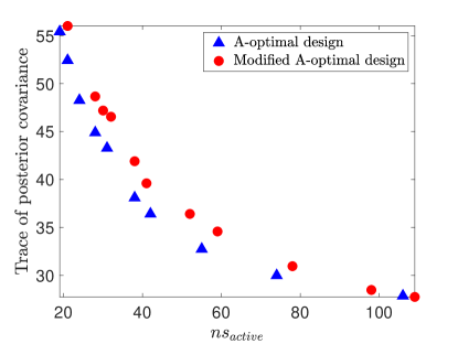
Figure 11: Comparison of designs obtained by minimizing the (approximate) A-optimal and modified A-optimal criteria. For each design, we report the exact trace of the corresponding posterior covariance operator.

7 Conclusion

We have established an efficient and flexible computational framework for A-optimal design of experiments in large-scale Bayesian linear inverse problems. The proposed randomized estimators for the OED objective and its gradient are accurate, efficient, simple to implement and parallelize. Specifically, the randomized estimators exploit the low-rank structure in the inverse problem; namely, the low-rank structure of the prior-preconditioned data misfit Hessian—a common feature of ill-posed inverse problems. Our reweighted $\ell_{1}$-minimization strategy is tailored to sensor placement problems, where finding binary optimal design vectors is desirable. We also presented the modified A-optimal criterion, which is more computationally efficient to compute and can provide designs that, while sub-optimal if the goal is to compute A-optimal designs, provide a systematic means for obtaining sensor placements with small posterior uncertainty levels.

Open questions that we seek to explore in our future work include adaptive determination of the target rank $k$ within the optimization algorithm, to further reduce computational costs, while ensuring sufficiently accurate estimates of the OED objective and gradient. Another possible line of inquiry is to use different low-rank approximations, such as Nyström’s method, and extending the randomized estimators to approximate trace of matrix functions. We also seek to incorporate the randomized estimators in a suitable optimization framework for Bayesian nonlinear inverse problems, in our future work.

Appendix A Proofs of bounds

A.1 Trace of matrix function

In the proofs below, we use the Loewner partial ordering [15, Chapter 7.7]; we briefly recapitulate some main results that will be useful in our proof. Let $\mathbf{A},\mathbf{B}\in\mathbb{R}^{n\times n}$ be symmetric positive definite; then $\mathbf{A}\preceq\mathbf{B}$ means that $\mathbf{B}-\mathbf{A}$ is positive semidefinite. For any $\mathbf{S}\in\mathbb{R}^{n\times m}$, it also follows that $\mathbf{S}^{\top}\mathbf{A}\mathbf{S}\preceq\mathbf{S}^{\top}\mathbf{B}\mathbf{S}$. Let $\mathbf{U}\mathbf{\Lambda}\mathbf{U}^{\top}$ be the eigendecomposition of $\mathbf{A}$. Then, $f(\mathbf{A})=\mathbf{U}f(\mathbf{\Lambda})\mathbf{U}^{\top}$ and $\mathsf{tr}\,\left(f(\mathbf{A})\right)=\sum_{i=1}^{n}f(\lambda_{i})$. If $f$ is monotonically increasing then $\mathsf{tr}\,\left(f(\mathbf{A})\right)\leq\mathsf{tr}\,\left(f(\mathbf{B})\right)$ since $\mathbf{A}\preceq\mathbf{B}$ implies $\lambda_{i}(\mathbf{A})\leq\lambda_{i}(\mathbf{B})$ for $i=1,\dots,n$.

The following bound allows us to bound the trace of a matrix function in terms of its diagonal subblocks.

Lemma 1.

Let

$$\mathbf{A}=\begin{bmatrix}\mathbf{A}_{11}&\mathbf{A}_{12}\\ \mathbf{A}_{12}^{\top}&\mathbf{A}_{22}\end{bmatrix}$$

be a symmetric positive definite matrix. Let $f$ be a nonnegative concave function on $[0,\infty)$. Then

$$\mathsf{tr}\,\left(f(\mathbf{A})\right)\leq\mathsf{tr}\,\left(f(\mathbf{A}_{11})\right)+\mathsf{tr}\,\left(f(\mathbf{A}_{22})\right).$$

Proof A.1.

See Theorem 2.1 and Remark 2.4 in [18].

We are ready to state and prove our main result of this section, which is the key in proving Theorem 3.1 and 5.1.

Theorem 2.

Let $\mathbf{A}\in\mathbb{R}^{n\times n}$ be a symmetric positive definite matrix with eigendecomposition

$$\mathbf{A}=\mathbf{U}\Lambda\mathbf{U}^{\top}=\begin{bmatrix}\mathbf{U}_{1}&\mathbf{U}_{2}\end{bmatrix}\begin{bmatrix}\mathbf{\Lambda}_{1}\\ &\mathbf{\Lambda}_{2}\end{bmatrix}\begin{bmatrix}\mathbf{U}_{1}^{\top}\\ \mathbf{U}_{2}^{\top}\end{bmatrix},$$

where $\mathbf{\Lambda}_{1}=\mathsf{diag}\,(\lambda_{1},\dots,\lambda_{k})$ and $\mathbf{\Lambda}_{2}=\mathsf{diag}\,(\lambda_{k+1},\dots,\lambda_{n})$ contain the eigenvalues arranged in descending order. Assume that the eigenvalue ratio $\gamma_{k}\equiv\frac{\lambda_{k+1}}{\lambda_{k}}<1$. Let $k$ be the target rank, $p\geq 2$ be the oversampling parameter such that $\ell\equiv k+p\leq n$, and let $q\geq 1$ be the number of subspace iterations. Furthermore, assume that $\mathbf{Q}\in\mathbb{R}^{n\times\ell}$ and $\mathbf{T}\in\mathbb{R}^{\ell\times\ell}$ are computed using Algorithm 1 and define $\widehat{\mathbf{A}}\equiv\mathbf{Q}\mathbf{T}\mathbf{Q}^{\top}$. Then

$$0\leq\mathbb{E}\left[\mathsf{tr}\,\left((\mathbf{I}+\widehat{\mathbf{A}})^{-1}\right)-\mathsf{tr}\,\left((\mathbf{I}+\mathbf{A})^{-1}\right)\right]\leq \>\mathsf{tr}\,\left(f(\mathbf{\Lambda}_{2})\right)+\mathsf{tr}\,\left(f(\gamma_{k}^{2q-1}C\mathbf{\Lambda}_{2})\right),$$

where $f=x/(1+x)$, and the constant $C$ is defined in Eq. 16.

Proof A.2.

Suppose $\text{rank}(\mathbf{A})=r$. Then, $\mathbf{A}$ has at most $r$ nonzero eigenvalues, and thus, we can define $\mathbf{\Lambda}_{r-k}=\text{diag}(\lambda_{k+1},\dots,\lambda_{r})$ so that

(30) $$\mathbf{\Lambda}_{2}=\begin{bmatrix}\mathbf{\Lambda}_{r-k}\\ &\mathbf{0}_{n-r-k}\end{bmatrix}.$$

We split this proof into several steps.

Step 0: Lower bound

Let $\tilde{\lambda}_{1}\geq\dots\geq\tilde{\lambda}_{\ell}\geq 0$ be the eigenvalues of $\mathbf{T}$ (and also $\widehat{\mathbf{A}}$). By the Cauchy interlacing theorem (see [20, Lemma 1] for the specific version of the argument), $\lambda_{i}\geq\tilde{\lambda}_{i}$ for $i=1,\dots,\ell$. Using properties of the trace operator

$$\mathsf{tr}\,\left((\mathbf{I}+\widehat{\mathbf{A}})^{-1}\right)-\mathsf{tr}\,\left((\mathbf{I}+\mathbf{A})^{-1}\right)= \>\sum_{i=1}^{\ell}\frac{1}{1+\tilde{\lambda}_{i}}+(n-\ell)-\sum_{i=1}^{n}\frac{1}{1+\lambda_{i}}$$

$$= \>\sum_{i=1}^{\ell}\frac{\lambda_{i}-\tilde{\lambda}_{i}}{(1+\lambda_{i})(1+\tilde{\lambda}_{i})}+\sum_{i=\ell+1}^{n}\frac{\lambda_{i}}{1+\lambda_{i}}.$$

Since each term in the summation is nonnegative, the lower bound follows.

Step 1. Trace of matrix function

We first write $\widehat{\mathbf{A}}=\mathbf{Q}\mathbf{T}\mathbf{Q}^{\top}=\mathbf{Q}\mathbf{Q}^{\top}\mathbf{A}\mathbf{Q}\mathbf{Q}^{\top}=\mathbf{P}_{\mathbf{Q}}\mathbf{A}\mathbf{P}_{\mathbf{Q}}$, where $\mathbf{P}_{\mathbf{Q}}=\mathbf{Q}\mathbf{Q}^{\top}$ is an orthogonal projection matrix onto the range of $\mathbf{Q}$. Since $\widehat{\mathbf{A}}$ has the same eigenvalues as $\mathbf{R}\equiv\mathbf{A}^{1/2}\mathbf{P}_{\mathbf{Q}}\mathbf{A}^{1/2}$ [15, Theorem 1.3.22],

(31) $$\mathsf{tr}\,\left((\mathbf{I}+\widehat{\mathbf{A}})^{-1}\right)=\mathsf{tr}\,\left((\mathbf{I}+\mathbf{A}^{1/2}\mathbf{P}_{\mathbf{Q}}\mathbf{A}^{1/2})^{-1}\right).$$

Also, since $\mathbf{P}_{\mathbf{Q}}\preceq\mathbf{I}$, it follows that $\mathbf{R}=\mathbf{A}^{1/2}\mathbf{P}_{\mathbf{Q}}\mathbf{A}^{1/2}\preceq\mathbf{A}$ and $\mathbf{0}\preceq\mathbf{A}-\mathbf{R}$. Therefore, from the proof of [5, Lemma X.1.4] and Eq. 31,

$$\mathsf{tr}\,\left((\mathbf{I}+\widehat{\mathbf{A}})^{-1}\right)-\mathsf{tr}\,\left((\mathbf{I}+\mathbf{A})^{-1}\right)\leq\mathsf{tr}\,\left(\left(\mathbf{I}-(\mathbf{I}+\mathbf{A}-\mathbf{R})^{-1}\right)\right)=\mathsf{tr}\,\left(f(\mathbf{A}-\mathbf{R})\right),$$

where $f(x)$ was defined in the statement of the theorem.

Step 2. Reducing the dimensionality

Let $\mathbf{F}_{\mathbf{S}}\equiv\mathbf{\Lambda}_{2}^{q}\boldsymbol{\Omega}_{2}\boldsymbol{\Omega}_{1}^{\dagger}\mathbf{\Lambda}^{-q}$. In Algorithm 1, we compute $\mathbf{Y}=\mathbf{A}^{q}\boldsymbol{\Omega}$ and let $\mathbf{Y}=\mathbf{Q}\mathbf{R}_{\mathbf{Y}}$ be the thin QR factorization of $\mathbf{Y}$. Let $\mathbf{W}_{\mathbf{Q}}=\mathbf{R}_{\mathbf{Y}}\boldsymbol{\Omega}_{1}^{\dagger}\mathbf{\Lambda}_{1}^{-q}(\mathbf{I}+\mathbf{F}_{\mathbf{S}}^{\top}\mathbf{F}_{\mathbf{S}})^{-1/2}\in\mathbb{R}^{\ell\times k}$ be defined as in the proof of [20, Theorem 6]. It was also shown that $\mathbf{W}_{\mathbf{Q}}$ has orthonormal columns, so that

$$\mathbf{Q}\mathbf{W}_{\mathbf{Q}}=\mathbf{U}\begin{bmatrix}\mathbf{I}\\ \mathbf{F}_{\mathbf{S}}\end{bmatrix}(\mathbf{I}+\mathbf{F}_{\mathbf{S}}^{\top}\mathbf{F}_{\mathbf{S}})^{-1/2}\in\mathbb{R}^{n\times k},$$

has orthonormal columns. The following sequence of identities also hold: $\mathbf{W}_{\mathbf{Q}}\mathbf{W}_{\mathbf{Q}}^{\top}\preceq\mathbf{I}$, $\mathbf{Q}\mathbf{W}_{\mathbf{Q}}\mathbf{W}_{\mathbf{Q}}^{\top}\mathbf{Q}^{\top}\preceq\mathbf{Q}\mathbf{Q}^{\top}$, and

$$\mathbf{A}-\mathbf{R}\preceq\mathbf{A}-\mathbf{A}^{1/2}\mathbf{Q}\mathbf{W}_{\mathbf{Q}}\mathbf{W}_{\mathbf{Q}}^{\top}\mathbf{Q}^{\top}\mathbf{A}^{1/2}\equiv\mathbf{S}.$$

Since $f(x)$ is a monotonic increasing function, $\mathsf{tr}\,\left(f(\mathbf{A}-\mathbf{R})\right)\leq\mathsf{tr}\,\left(f(\mathbf{S})\right)$.

Step 3. Split into the diagonal blocks

We can rewrite $\mathbf{S}$ as

$$\mathbf{S}=\mathbf{U}\begin{bmatrix}\mathbf{S}_{1}&*\\ *&\mathbf{S}_{2}\end{bmatrix}\mathbf{U}^{\top},$$

where $*$ represents blocks that can be ignored and

$$\mathbf{S}_{1}\equiv\mathbf{\Lambda}_{1}^{1/2}(\mathbf{I}-(\mathbf{I}+\mathbf{F}_{\mathbf{S}}^{\top}\mathbf{F}_{\mathbf{S}})^{-1})\mathbf{\Lambda}_{1}^{1/2},\qquad\mathbf{S}_{2}=\mathbf{\Lambda}_{2}^{1/2}(\mathbf{I}-\mathbf{F}_{\mathbf{S}}(\mathbf{I}+\mathbf{F}^{\top}_{\mathbf{S}}\mathbf{F}_{\mathbf{S}})^{-1}\mathbf{F}_{\mathbf{S}}^{\top})\mathbf{\Lambda}_{2}^{1/2}.$$

We can invoke 1, since $f(x)=x/(1+x)$ is concave and nonnegative on $[0,\infty)$. Therefore, we have

$$\mathsf{tr}\,\left(f(\mathbf{S})\right)\leq\mathsf{tr}\,\left(f(\mathbf{S}_{1})\right)+\mathsf{tr}\,\left(f(\mathbf{S}_{2})\right).$$

Note that the matrix $\mathbf{U}$ disappears, because the trace is unitarily invariant.

Step 4. Completing the structural bound

Using an SVD based argument it can be shown that $\mathbf{I}-(\mathbf{I}+\mathbf{F}_{\mathbf{S}}^{\top}\mathbf{F}_{\mathbf{S}})^{-1}\preceq\mathbf{F}_{\mathbf{S}}^{\top}\mathbf{F}_{\mathbf{S}}$, so that

$$\mathbf{S}_{1}=\mathbf{\Lambda}_{1}^{1/2}(\mathbf{I}-(\mathbf{I}+\mathbf{F}_{\mathbf{S}}^{\top}\mathbf{F}_{\mathbf{S}})^{-1})\mathbf{\Lambda}_{1}^{1/2}\preceq\mathbf{\Lambda}_{1}^{1/2}\mathbf{F}_{\mathbf{S}}^{\top}\mathbf{F}_{\mathbf{S}}\mathbf{\Lambda}_{1}^{1/2}.$$

Therefore, since $f$ is monotonically increasing

(32) $$\mathsf{tr}\,\left(f(\mathbf{S}_{1})\right)\leq\>\mathsf{tr}\,\left(f(\mathbf{\Lambda}_{1}^{1/2}\mathbf{F}_{\mathbf{S}}^{\top}\mathbf{F}_{\mathbf{S}}\mathbf{\Lambda}_{1}^{1/2})\right)=\>\sum_{j=1}^{k}f\left(\lambda_{j}\left[\mathbf{\Lambda}_{1}^{1/2}\mathbf{F}_{\mathbf{S}}^{\top}\mathbf{F}_{\mathbf{S}}\mathbf{\Lambda}_{1}^{1/2}\right]\right).$$

Note that $\mathbf{F}_{\mathbf{S}}\mathbf{\Lambda}_{1}^{1/2}$ is $(n-k)\times k$ has at most $\min\{n-k,k\}$ nonzero singular values. Looking more into the structure of $\mathbf{F}_{\mathbf{S}}\mathbf{\Lambda}_{1}^{1/2}$, and using Eq. 30, we can write

$$\mathbf{F}_{\mathbf{S}}\mathbf{\Lambda}_{1}^{1/2}= \>\mathbf{\Lambda}_{2}^{1/2}\begin{bmatrix}\mathbf{\Lambda}_{r-k}^{q-1/2}\\ &\mathbf{0}\end{bmatrix}\boldsymbol{\Omega}_{2}\boldsymbol{\Omega}_{1}^{\dagger}\mathbf{\Lambda}_{1}^{-q+1/2}$$

$$= \>\mathbf{\Lambda}_{2}^{1/2}\begin{bmatrix}\mathbf{\Lambda}_{r-k}^{q-1/2}\widehat{\boldsymbol{\Omega}}_{2}\boldsymbol{\Omega}_{1}^{\dagger}\mathbf{\Lambda}_{1}^{-q+1/2}\\ \mathbf{0}\end{bmatrix},$$

where $\widehat{\boldsymbol{\Omega}}_{2}\in\mathbb{R}^{(r-k)\times(k+p)}$ such that $\boldsymbol{\Omega}_{2}=\begin{bmatrix}\widehat{\boldsymbol{\Omega}}_{2}\\ \mathbf{*}\end{bmatrix}$. Using the multiplicative singular value inequalities [15, Equation (7.3.14)] and repeated use of the submultiplicative inequality gives

(33) $$\sigma_{j}(\mathbf{F}_{\mathbf{S}}\mathbf{\Lambda}_{1}^{1/2})\leq\gamma_{k}^{q-1/2}\|\widehat{\boldsymbol{\Omega}}_{2}\boldsymbol{\Omega}_{1}^{\dagger}\|_{2}\sigma_{j}(\mathbf{\Lambda}_{2}^{1/2}),\qquad j=1,\dots,\min\{k,n-k\}.$$

The analysis splits into two cases:

Case 1: $k\leq n-k$.

Since $f$ is monotonically increasing, using Eqs. 32 and 33

$$\mathsf{tr}\,\left(f(\mathbf{S}_{1})\right)\leq \>\sum_{j=1}^{k}f\left(\lambda_{j}\left[\mathbf{\Lambda}_{1}^{1/2}\mathbf{F}_{\mathbf{S}}^{\top}\mathbf{F}_{\mathbf{S}}\mathbf{\Lambda}_{1}^{1/2}\right]\right)\leq\sum_{j=1}^{k}f\left(\gamma_{k}^{2q-1}\|\widehat{\boldsymbol{\Omega}}_{2}\boldsymbol{\Omega}_{1}^{\dagger}\|_{2}^{2}\sigma_{j}^{2}(\mathbf{\Lambda}_{2}^{1/2})\right)$$

$$\leq \>\sum_{j=1}^{n-k}f\left(\gamma_{k}^{2q-1}\|\widehat{\boldsymbol{\Omega}}_{2}\boldsymbol{\Omega}_{1}^{\dagger}\|_{2}^{2}\sigma_{j}^{2}(\mathbf{\Lambda}_{2}^{1/2})\right)=\mathsf{tr}\,\left(f(\gamma_{k}^{2q-1}\|\widehat{\boldsymbol{\Omega}}_{2}\boldsymbol{\Omega}_{1}^{\dagger}\|_{2}^{2}\mathbf{\Lambda}_{2})\right).$$

Case 2: $k>n-k$.

Since $\mathbf{\Lambda}_{1}^{1/2}\mathbf{F}_{\mathbf{S}}^{\top}\mathbf{F}_{\mathbf{S}}\mathbf{\Lambda}_{1}^{1/2}$ has at most $n-k$ nonzero eigenvalues, use the fact that $f(0)=0$, along with Eqs. 32 and 33 to obtain

$$\mathsf{tr}\,\left(f(\mathbf{S}_{1})\right)\leq \>\sum_{j=1}^{k}f\left(\lambda_{j}\left[\mathbf{\Lambda}_{1}^{1/2}\mathbf{F}_{\mathbf{S}}^{\top}\mathbf{F}_{\mathbf{S}}\mathbf{\Lambda}_{1}^{1/2}\right]\right)=\sum_{j=1}^{n-k}f\left(\lambda_{j}\left[\mathbf{\Lambda}_{1}^{1/2}\mathbf{F}_{\mathbf{S}}^{\top}\mathbf{F}_{\mathbf{S}}\mathbf{\Lambda}_{1}^{1/2}\right]\right)$$

$$\leq \>\sum_{j=1}^{n-k}f\left(\gamma_{k}^{2q-1}\|\widehat{\boldsymbol{\Omega}}_{2}\boldsymbol{\Omega}_{1}^{\dagger}\|_{2}^{2}\sigma_{j}^{2}(\mathbf{\Lambda}_{2}^{1/2})\right)=\mathsf{tr}\,\left(f(\gamma_{k}^{2q-1}\|\widehat{\boldsymbol{\Omega}}_{2}\boldsymbol{\Omega}_{1}^{\dagger}\|_{2}^{2}\mathbf{\Lambda}_{2})\right).$$

To summarize, in both cases $\mathsf{tr}\,\left(f(\mathbf{S}_{1})\right)\leq\mathsf{tr}\,\left(f(\gamma_{k}^{2q-1}\|\widehat{\boldsymbol{\Omega}}_{2}\boldsymbol{\Omega}_{1}^{\dagger}\|_{2}^{2}\mathbf{\Lambda}_{2})\right).$ Similarly, since $\mathbf{0}\preceq\mathbf{F}_{\mathbf{S}}(\mathbf{I}+\mathbf{F}_{\mathbf{S}}^{\top}\mathbf{F}_{\mathbf{S}})^{-1}\mathbf{F}_{\mathbf{S}}^{\top}$, we can show

$$\mathbf{S}_{2}=\>\mathbf{\Lambda}_{2}^{1/2}(\mathbf{I}-\mathbf{F}_{\mathbf{S}}(\mathbf{I}+\mathbf{F}_{\mathbf{S}}^{\top}\mathbf{F}_{\mathbf{S}})^{-1}\mathbf{F}_{\mathbf{S}}^{\top})\mathbf{\Lambda}_{2}^{1/2}\preceq\mathbf{\Lambda}_{2},$$

so that $\mathsf{tr}\,\left(f(\mathbf{S}_{2})\right)\leq\mathsf{tr}\,\left(f(\mathbf{\Lambda}_{2})\right)$. Combine with step 3 to obtain

$$\mathsf{tr}\,\left(f(\mathbf{S})\right)\leq\mathsf{tr}\,\left(f(\mathbf{\Lambda}_{2})\right)+\mathsf{tr}\,\left(f(\gamma_{k}^{2q-1}\|\widehat{\boldsymbol{\Omega}}_{2}\boldsymbol{\Omega}_{1}^{\dagger}\|_{2}^{2}\mathbf{\Lambda}_{2})\right).$$

Combine this with the results of steps 1 and 2, to obtain the structural bound

$$\mathsf{tr}\,\left((\mathbf{I}+\widehat{\mathbf{A}})^{-1}\right)-\mathsf{tr}\,\left((\mathbf{I}+\mathbf{A})^{-1}\right)\leq\mathsf{tr}\,\left(f(\gamma_{k}^{2q-1}\|\widehat{\boldsymbol{\Omega}}_{2}\boldsymbol{\Omega}_{1}^{\dagger}\|_{2}^{2}\mathbf{\Lambda}_{2})\right)+\mathsf{tr}\,\left(f(\mathbf{\Lambda}_{2})\right).$$

Step 5. The expectation bound

Note that $\widehat{\boldsymbol{\Omega}}_{2}\in\mathbb{R}^{(r-k)\times(k+p)}$ and $\boldsymbol{\Omega}_{1}\in\mathbb{R}^{k\times(k+p)}$. From the proof of [20, Theorem 1], we have $\mathbb{E}\,[\|\widehat{\boldsymbol{\Omega}}_{2}\boldsymbol{\Omega}_{1}^{\dagger}\|_{2}^{2}]\leq C$, where $C$ was defined in Eq. 16. By Jensen’s inequality, using the fact that $f(x)=x/(1+x)$ is concave on $[0,\infty)$ we have

$$\mathbb{E}\left[\mathsf{tr}\,\left((\mathbf{I}+\widehat{\mathbf{A}})^{-1}\right)-\mathsf{tr}\,\left((\mathbf{I}+\mathbf{A})^{-1}\right)\right]\leq \>\mathsf{tr}\,\left(f(\mathbf{\Lambda}_{2})\right)+\mathbb{E}\left[\mathsf{tr}\,\left(f(\gamma_{k}^{2q-1}\|\widehat{\boldsymbol{\Omega}}_{2}\boldsymbol{\Omega}_{1}^{\dagger}\|_{2}^{2}\mathbf{\Lambda}_{2})\right)\right]$$

$$\leq \>\mathsf{tr}\,\left(f(\mathbf{\Lambda}_{2})\right)+\mathsf{tr}\,\left(f(\gamma_{k}^{2q-1}C\mathbf{\Lambda}_{2})\right).$$

Combining this with the lower bound (step 0) completes the proof.

A.2 Proof of Theorem 3.1

For the remaining discussion, recall the notation from Theorem 3.1

(34) $$\mathbf{P}_{j}={\mathbfcal{F}}^{\top}\mathbf{E}_{j}^{\text{noise}}{\mathbfcal{F}},$$

where ${\mathbfcal{F}}$ and $\mathbf{E}_{j}^{\text{noise}}$ are defined in Eq. 3 and Eq. 6, respectively. We will also need

Lemma 3 (See [3]).

Let $\mathbf{A},\mathbf{B}\in\mathbb{R}^{n\times n}$ and let $\mathbf{B}$ be a symmetric positive semidefinite matrix. Then, we have $|\mathsf{tr}\,\left(\mathbf{A}\mathbf{B}\right)|\leq\|\mathbf{A}\|_{2}\mathsf{tr}\,\left(\mathbf{B}\right)$.

Proof A.3 ( Theorem 3.1).

Recall our estimator $\widehat{\Phi}_{\text{aopt}}{({\mathchoice{\mbox{\boldmath$\displaystyle{w}$}}{\mbox{\boldmath$\textstyle{w}$}}{\mbox{\boldmath$\scriptstyle{w}$}}{\mbox{\boldmath$\scriptscriptstyle{w}$}}};\ell)}$ from Eq. 11. For fixed $\ell$, using 3 we have

$$\begin{aligned} \mathbb{E}|\Phi_{\text{aopt}}{({\mathchoice{\mbox{\boldmath$\displaystyle{w}$}}{\mbox{\boldmath$\textstyle{w}$}}{\mbox{\boldmath$\scriptstyle{w}$}}{\mbox{\boldmath$\scriptscriptstyle{w}$}}})}-\widehat{\Phi}_{\text{aopt}}{({\mathchoice{\mbox{\boldmath$\displaystyle{w}$}}{\mbox{\boldmath$\textstyle{w}$}}{\mbox{\boldmath$\scriptstyle{w}$}}{\mbox{\boldmath$\scriptscriptstyle{w}$}}};\ell)}|=&\>\mathbb{E}\left|\mathsf{tr}\,\left((\mathbf{I}+\mathbfcal{H}_{\text{m}}({\mathchoice{\mbox{\boldmath$\displaystyle{w}$}}{\mbox{\boldmath$\textstyle{w}$}}{\mbox{\boldmath$\scriptstyle{w}$}}{\mbox{\boldmath$\scriptscriptstyle{w}$}}}))^{-1}\mathbf{Z}-(\mathbf{I}+\widehat{\mathbfcal{H}}_{\text{m}}({\mathchoice{\mbox{\boldmath$\displaystyle{w}$}}{\mbox{\boldmath$\textstyle{w}$}}{\mbox{\boldmath$\scriptstyle{w}$}}{\mbox{\boldmath$\scriptscriptstyle{w}$}}}))^{-1}\mathbf{Z}\right)\right|\\ \leq&\>\|\mathbf{Z}\|_{2}\mathbb{E}|\mathsf{tr}\,\left((\mathbf{I}+\mathbfcal{H}_{\text{m}}({\mathchoice{\mbox{\boldmath$\displaystyle{w}$}}{\mbox{\boldmath$\textstyle{w}$}}{\mbox{\boldmath$\scriptstyle{w}$}}{\mbox{\boldmath$\scriptscriptstyle{w}$}}}))^{-1}-(\mathbf{I}+\widehat{\mathbfcal{H}}_{\text{m}}({\mathchoice{\mbox{\boldmath$\displaystyle{w}$}}{\mbox{\boldmath$\textstyle{w}$}}{\mbox{\boldmath$\scriptstyle{w}$}}{\mbox{\boldmath$\scriptscriptstyle{w}$}}}))^{-1}\right)|.\end{aligned}.$$

Applying 2 establishes Eq. 17.

Next, we consider Eq. 18. Recall the estimator $\widehat{\partial_{j}\Phi}_{\text{aopt}}{({\mathchoice{\mbox{\boldmath$\displaystyle{w}$}}{\mbox{\boldmath$\textstyle{w}$}}{\mbox{\boldmath$\scriptstyle{w}$}}{\mbox{\boldmath$\scriptscriptstyle{w}$}}};\ell)}$ from Eq. 12. We can write the absolute error as

$$|\partial_{j}\Phi_{\text{aopt}}{({\mathchoice{\mbox{\boldmath$\displaystyle{w}$}}{\mbox{\boldmath$\textstyle{w}$}}{\mbox{\boldmath$\scriptstyle{w}$}}{\mbox{\boldmath$\scriptscriptstyle{w}$}}})}-\widehat{\partial_{j}\Phi}_{\text{aopt}}{({\mathchoice{\mbox{\boldmath$\displaystyle{w}$}}{\mbox{\boldmath$\textstyle{w}$}}{\mbox{\boldmath$\scriptstyle{w}$}}{\mbox{\boldmath$\scriptscriptstyle{w}$}}};\ell)}|\\ =|\mathsf{tr}\,\left(\big{(}(\mathbf{I}+\mathbfcal{H}_{\text{m}}({\mathchoice{\mbox{\boldmath$\displaystyle{w}$}}{\mbox{\boldmath$\textstyle{w}$}}{\mbox{\boldmath$\scriptstyle{w}$}}{\mbox{\boldmath$\scriptscriptstyle{w}$}}}))^{-1}\mathbf{P}_{j}(\mathbf{I}+\mathbfcal{H}_{\text{m}}({\mathchoice{\mbox{\boldmath$\displaystyle{w}$}}{\mbox{\boldmath$\textstyle{w}$}}{\mbox{\boldmath$\scriptstyle{w}$}}{\mbox{\boldmath$\scriptscriptstyle{w}$}}}))^{-1}-(\mathbf{I}+\widehat{\mathbfcal{H}}_{\text{m}}({\mathchoice{\mbox{\boldmath$\displaystyle{w}$}}{\mbox{\boldmath$\textstyle{w}$}}{\mbox{\boldmath$\scriptstyle{w}$}}{\mbox{\boldmath$\scriptscriptstyle{w}$}}}))^{-1}{\mathbf{P}}_{j}(\mathbf{I}+\widehat{\mathbfcal{H}}_{\text{m}}({\mathchoice{\mbox{\boldmath$\displaystyle{w}$}}{\mbox{\boldmath$\textstyle{w}$}}{\mbox{\boldmath$\scriptstyle{w}$}}{\mbox{\boldmath$\scriptscriptstyle{w}$}}}))^{-1}\big{)}\mathbf{Z}\right)|,$$

where $\widehat{\mathbfcal{H}}_{\text{m}}({\mathchoice{\mbox{\boldmath$\displaystyle{w}$}}{\mbox{\boldmath$\textstyle{w}$}}{\mbox{\boldmath$\scriptstyle{w}$}}{\mbox{\boldmath$\scriptscriptstyle{w}$}}})=\mathbf{Q}\mathbf{T}\mathbf{Q}^{\top}.$ We use the decomposition

$$\big{(}(\mathbf{I}+\mathbfcal{H}_{\text{m}}({\mathchoice{\mbox{\boldmath$\displaystyle{w}$}}{\mbox{\boldmath$\textstyle{w}$}}{\mbox{\boldmath$\scriptstyle{w}$}}{\mbox{\boldmath$\scriptscriptstyle{w}$}}}))^{-1}\mathbf{P}_{j}(\mathbf{I}+\mathbfcal{H}_{\text{m}}({\mathchoice{\mbox{\boldmath$\displaystyle{w}$}}{\mbox{\boldmath$\textstyle{w}$}}{\mbox{\boldmath$\scriptstyle{w}$}}{\mbox{\boldmath$\scriptscriptstyle{w}$}}}))^{-1}-(\mathbf{I}+\widehat{\mathbfcal{H}}_{\text{m}}({\mathchoice{\mbox{\boldmath$\displaystyle{w}$}}{\mbox{\boldmath$\textstyle{w}$}}{\mbox{\boldmath$\scriptstyle{w}$}}{\mbox{\boldmath$\scriptscriptstyle{w}$}}}))^{-1}{\mathbf{P}}_{j}(\mathbf{I}+\widehat{\mathbfcal{H}}_{\text{m}}({\mathchoice{\mbox{\boldmath$\displaystyle{w}$}}{\mbox{\boldmath$\textstyle{w}$}}{\mbox{\boldmath$\scriptstyle{w}$}}{\mbox{\boldmath$\scriptscriptstyle{w}$}}}))^{-1}\big{)}\mathbf{Z}\\ =-\left(\mathbf{D}\mathbf{P}_{j}(\mathbf{I}+\mathbfcal{H}_{\text{m}}({\mathchoice{\mbox{\boldmath$\displaystyle{w}$}}{\mbox{\boldmath$\textstyle{w}$}}{\mbox{\boldmath$\scriptstyle{w}$}}{\mbox{\boldmath$\scriptscriptstyle{w}$}}}))^{-1}+(\mathbf{I}+\widehat{\mathbfcal{H}}_{\text{m}}({\mathchoice{\mbox{\boldmath$\displaystyle{w}$}}{\mbox{\boldmath$\textstyle{w}$}}{\mbox{\boldmath$\scriptstyle{w}$}}{\mbox{\boldmath$\scriptscriptstyle{w}$}}}))^{-1}\mathbf{P}_{j}\mathbf{D}\right)\mathbf{Z},$$

where $\mathbf{D}\equiv(\mathbf{I}+\widehat{\mathbfcal{H}}_{\text{m}}({\mathchoice{\mbox{\boldmath$\displaystyle{w}$}}{\mbox{\boldmath$\textstyle{w}$}}{\mbox{\boldmath$\scriptstyle{w}$}}{\mbox{\boldmath$\scriptscriptstyle{w}$}}}))^{-1}-(\mathbf{I}+\mathbfcal{H}_{\text{m}}({\mathchoice{\mbox{\boldmath$\displaystyle{w}$}}{\mbox{\boldmath$\textstyle{w}$}}{\mbox{\boldmath$\scriptstyle{w}$}}{\mbox{\boldmath$\scriptscriptstyle{w}$}}}))^{-1}$. Repeated application of 3 gives

$$|\partial_{j}\Phi_{\text{aopt}}{({\mathchoice{\mbox{\boldmath$\displaystyle{w}$}}{\mbox{\boldmath$\textstyle{w}$}}{\mbox{\boldmath$\scriptstyle{w}$}}{\mbox{\boldmath$\scriptscriptstyle{w}$}}})}-\partial_{j}\widehat{\Phi}_{\text{aopt}}{({\mathchoice{\mbox{\boldmath$\displaystyle{w}$}}{\mbox{\boldmath$\textstyle{w}$}}{\mbox{\boldmath$\scriptstyle{w}$}}{\mbox{\boldmath$\scriptscriptstyle{w}$}}};\ell)}|\leq \>\|\mathbf{P}_{j}\|_{2}\|\mathbf{Z}\|_{2}\left(\|(\mathbf{I}+\mathbfcal{H}_{\text{m}}({\mathchoice{\mbox{\boldmath$\displaystyle{w}$}}{\mbox{\boldmath$\textstyle{w}$}}{\mbox{\boldmath$\scriptstyle{w}$}}{\mbox{\boldmath$\scriptscriptstyle{w}$}}}))^{-1}\|_{2}+\right.$$

$$\>\qquad~{}~{}~{}~{}~{}~{}~{}~{}~{}~{}~{}~{}~{}~{}~{}~{}~{}~{}~{}~{}~{}\left.\|(\mathbf{I}+\widehat{\mathbfcal{H}}_{\text{m}}({\mathchoice{\mbox{\boldmath$\displaystyle{w}$}}{\mbox{\boldmath$\textstyle{w}$}}{\mbox{\boldmath$\scriptstyle{w}$}}{\mbox{\boldmath$\scriptscriptstyle{w}$}}}))^{-1}\|_{2}\right)\mathsf{tr}\,\left(\mathbf{D}\right).$$

Since $\mathbf{I}+\mathbfcal{H}_{\text{m}}({\mathchoice{\mbox{\boldmath$\displaystyle{w}$}}{\mbox{\boldmath$\textstyle{w}$}}{\mbox{\boldmath$\scriptstyle{w}$}}{\mbox{\boldmath$\scriptscriptstyle{w}$}}})$ and $\mathbf{I}+\widehat{\mathbfcal{H}}_{\text{m}}({\mathchoice{\mbox{\boldmath$\displaystyle{w}$}}{\mbox{\boldmath$\textstyle{w}$}}{\mbox{\boldmath$\scriptstyle{w}$}}{\mbox{\boldmath$\scriptscriptstyle{w}$}}})$ have eigenvalues greater than or equal to one, $\|(\mathbf{I}+\mathbfcal{H}_{\text{m}}({\mathchoice{\mbox{\boldmath$\displaystyle{w}$}}{\mbox{\boldmath$\textstyle{w}$}}{\mbox{\boldmath$\scriptstyle{w}$}}{\mbox{\boldmath$\scriptscriptstyle{w}$}}}))^{-1}\|_{2}+\|(\mathbf{I}+\widehat{\mathbfcal{H}}_{\text{m}}({\mathchoice{\mbox{\boldmath$\displaystyle{w}$}}{\mbox{\boldmath$\textstyle{w}$}}{\mbox{\boldmath$\scriptstyle{w}$}}{\mbox{\boldmath$\scriptscriptstyle{w}$}}}))^{-1}\|_{2}\leq 2$. Finally, taking the expectation and applying 2, we have the desired result.

A.3 Proof of Theorem 5.1

Proof A.4.

The proof follows in similar lines as the proof of Theorem 3.1 except the fact that in Theorem 5.1 we do not have $\mathbf{Z}$ in the expressions.

References

- [1] A. Alexanderian, P. J. Gloor, O. Ghattas, et al., On Bayesian A-and D-optimal experimental designs in infinite dimensions, Bayesian Analysis, 11 (2016), pp. 671–695.
- [2] A. Alexanderian, N. Petra, G. Stadler, and O. Ghattas, A-optimal design of experiments for infinite-dimensional Bayesian linear inverse problems with regularized -sparsification, SIAM Journal on Scientific Computing, 36 (2014), pp. pp. A2122 – A2148.
- [3] A. Alexanderian and A. K. Saibaba, Efficient D-optimal design of experiments for infinite-dimensional Bayesian linear inverse problems, SIAM Journal on Scientific Computing, (2018).
- [4] A. Attia, A. Alexanderian, and A. K. Saibaba, Goal-oriented optimal design of experiments for large-scale Bayesian linear inverse problems, Inverse Problems, 34 (2018), p. 095009.
- [5] R. Bhatia, Matrix analysis, vol. 169 of Graduate Texts in Mathematics, Springer-Verlag, New York, 1997.
- [6] T. Bui-Thanh, O. Ghattas, J. Martin, and G. Stadler, A computational framework for infinite-dimensional Bayesian inverse problems Part I: The linearized case, with application to global seismic inversion, SIAM Journal on Scientific Computing, 35 (2013), pp. A2494–A2523.
- [7] E. J. Candès, M. B. Wakin, and S. P. Boyd, Enhancing sparsity by reweighted minimization, Journal of Fourier Analysis and Applications, 14 (2008), pp. 877–905.
- [8] K. Chaloner and I. Verdinelli, Bayesian experimental design: A review, Statistical Science, (1995), pp. 273–304.
- [9] M. Dashti and A. M. Stuart, The Bayesian approach to inverse problems, in Handbook of Uncertainty Quantification, R. Ghanem, D. Higdon, and H. Owhadi, eds., Spinger, 2017.
- [10] J. Fohring and E. Haber, Adaptive A-optimal experimental design for linear dynamical systems, SIAM-ASA Journal on Uncertainty Quantification, 4 (2016), pp. 1138–1159.
- [11] E. Haber, L. Horesh, and L. Tenorio, Numerical methods for experimental design of large-scale linear ill-posed inverse problems, Inverse Problems, 24 (2008), pp. 125–137.
- [12] E. Haber, L. Horesh, and L. Tenorio, Numerical methods for the design of large-scale nonlinear discrete ill-posed inverse problems, Inverse Problems, 26 (2010), p. 025002.
- [13] E. Haber, Z. Magnant, C. Lucero, and L. Tenorio, Numerical methods for A-optimal designs with a sparsity constraint for ill-posed inverse problems, Computational Optimization and Applications, (2012), pp. 1–22.
- [14] N. Halko, P.-G. Martinsson, and J. A. Tropp, Finding structure with randomness: Probabilistic algorithms for constructing approximate matrix decompositions, SIAM review, 53 (2011), pp. 217–288.
- [15] R. A. Horn and C. R. Johnson, Matrix Analysis, Cambridge University Press, Cambridge, second ed., 2013.
- [16] D. R. Hunter and K. Lange, A tutorial on MM algorithms, The American Statistician, 58 (2004), pp. 30–37.
- [17] K. Lange, MM optimization algorithms, vol. 147, SIAM, 2016.
- [18] E.-Y. Lee, Extension of Rotfel’d theorem, Linear Algebra and its Applications, 435 (2011), pp. 735–741.
- [19] C. D. Meyer, Matrix Analysis and Applied Linear Algebra, Other Titles in Applied Mathematics, Society for Industrial and Applied Mathematics, 2000.
- [20] A. K. Saibaba, A. Alexanderian, and I. C. F. Ipsen, Randomized matrix-free trace and log-determinant estimators, Numerische Mathematik, 137 (2017).
- [21] A. M. Stuart, Inverse problems: A Bayesian perspective, Acta Numerica, 19 (2010), pp. 451–559.
- [22] D. Uciński, Optimal Measurement Methods for Distributed Parameter System Identification, CRC Press, Boca Raton, 2005.
- [23] J. Yu, V. M. Zavala, and M. Anitescu, A scalable design of experiments framework for optimal sensor placement, Journal of Process Control, 67 (2018), pp. 44–55.