Improving Neural Language Modeling via Adversarial Training

Abstract

Recently, substantial progress has been made in language modeling by using deep neural networks. However, in practice, large scale neural language models have been shown to be prone to overfitting. In this paper, we present a simple yet highly effective adversarial training mechanism for regularizing neural language models. The idea is to introduce adversarial noise to the output embedding layer while training the models. We show that the optimal adversarial noise yields a simple closed form solution, thus allowing us to develop a simple and time efficient algorithm. Theoretically, we show that our adversarial mechanism effectively encourages the diversity of the embedding vectors, helping to increase the robustness of models. Empirically, we show that our method improves on the single model state-of-the-art results for language modeling on Penn Treebank (PTB) and Wikitext-2, achieving test perplexity scores of 46.01 and 38.07, respectively. When applied to machine translation, our method improves over various transformer-based translation baselines in BLEU scores on the WMT14 English-German and IWSLT14 German-English tasks.

1 Introduction

Statistical language modeling is a fundamental task in machine learning, with wide applications in various areas, including automatic speech recognition (e.g., Yu & Deng, 2016), machine translation (e.g., Koehn, 2009) and computer vision (e.g., Xu et al., 2015), to name a few. Recently, deep neural network models, especially recurrent neural networks (RNN) based models, have emerged to be one of the most powerful approaches for language modeling (e.g., Merity et al., 2018a; Yang et al., 2018; Vaswani et al., 2017; Anderson et al., 2018).

Unfortunately, a major challenge in training large scale RNN-based language models is their tendency to overfit; this is caused by the high complexity of RNN models and the discrete nature of language inputs. Although various regularization techniques, such as early stop and dropout (e.g., Gal & Ghahramani, 2016), have been investigated, severe overfitting is still widely observed in state-of-the-art benchmarks, as evidenced by the large gap between training and testing performance.

In this paper, we develop a simple yet surprisingly efficient minimax training strategy for regularization. Our idea is to inject an adversarial perturbation on the word embedding vectors in the softmax layer of the language models, and seek to find the optimal parameters that maximize the worst-case performance subject to the adversarial perturbation. Importantly, we show that the optimal perturbation vectors yield a simple and computationally efficient form under our construction, allowing us to derive a simple and fast training algorithm (see Algorithm 1), which can be easily implemented based a minor modification of the standard maximum likelihood training and does not introduce additional training parameters.

An intriguing theoretical property of our method is that it provides an effective mechanism to encourage diversity of word embedding vectors, which is widely observed to yield better generalization performance in neural language models (e.g., Mu et al., 2018; Gao et al., 2019; Liu et al., 2018b; Cogswell et al., 2016; Khodak et al., 2018). In previous works, the diversity is often enforced explicitly by adding additional diversity penalty terms (e.g., Gao et al., 2019), which may impact the likelihood optimization and are computationally expensive when the vocabulary size is large. Interestingly, we show that our adversarial training effectively enforces diversity without explicitly introducing the additional diversity penalty, and is significantly more computationally efficient than direct regularizations.

Empirically, we find that our adversarial method can significantly improve the performance of state-of-the-art large-scale neural language modeling and machine translation. For language modeling, we establish a new single model state-of-the-art result for the Penn Treebank (PTB) and WikiText-2 (WT2) datasets to the best of our knowledge, achieving 46.01 and 38.07 test perplexity scores, respectively. On the large scale WikiText-103 (WT3) dataset, our method improves the Quasi-recurrent neural networks (QRNNs) (Merity et al., 2018b) baseline.

To demonstrate the broad applicability of the method, we also apply our method to improve machine translation, using Transformer (Vaswani et al., 2017) as our base model. By incorporating our adversarial training, we improve a variety of Transformer-based translation baselines on the WMT2014 English-German and IWSTL2014 German-English translations.

2 Background: Neural Language Modeling

Typical word-level language models are specified as a product of conditional probabilities using the chain rule:

$$p(x_{1:T})=\prod_{t=1}^{T}p(x_{t}~{}|~{}x_{1:t-1}),$$ (1)

where $x_{1:T}=[x_{1},\cdots,x_{T}]$ denotes a sentence of length $T$, with $x_{t}\in{\mathcal{V}}$ the $t$-th word and ${\mathcal{V}}$ the vocabulary set. In modern deep language models, the conditional probabilities $p(x_{t}|x_{1:t-1})$ are often specified using recurrent neural networks (RNNs), in which the context $x_{1:t-1}$ at each time $t$ is represented using a hidden state vector $h_{t}\in\mathbb{R}^{d_{h}}$ defined recursively via

$$h_{t}=f(x_{t-1},h_{t-1};\boldsymbol{\theta}),$$ (2)

where $f$ is a nonlinear map with a trainable parameter $\boldsymbol{\theta}$. The conditional probabilities are then defined using a softmax function:

$$\begin{split}p(x_{t}~{}|~{}x_{1:t-1};\boldsymbol{\theta},\boldsymbol{w})&={\mathrm{Softmax}}(x_{t},\boldsymbol{w},h_{t})\\ &:=\frac{\exp(w_{x_{t}}^{\top}h_{t})}{\sum_{\ell=1}^{|\mathcal{V}|}\exp(w_{\ell}^{\top}h_{t})},\end{split}$$ (3)

where $\boldsymbol{w}=\{w_{i}\}\subset\mathbb{R}^{d}$ is the coefficient of softmax; $w_{i}$ can be viewed as an embedding vector for word $i\in\mathcal{V}$ and $h_{t}$ the embedding vector of context $x_{1:t-1}$. The inner product $w_{x_{t}}^{\top}h_{t}$ measures the similarity between word $x_{t}$ and context $x_{1:t-1}$, which is converted into a probability using the softmax function.

In practice, the nonlinear map $f$ is specified by typical RNN units, such as LSTM (Hochreiter & Schmidhuber, 1997) or GRU (Chung et al., 2014), applied on another set of embedding vectors $w_{i}^{\prime}\in\mathbb{R}^{d^{\prime}}$ of the words, that is,

$$f(x_{t-1},h_{t-1};~{}\boldsymbol{\theta})=f_{RNN}(w^{\prime}_{x_{t-1}},h_{t-1};~{}\boldsymbol{\theta}^{\prime}),$$

where $\boldsymbol{\theta}^{\prime}$ is the weight of the RNN unit $f_{RNN}$, and $\boldsymbol{\theta}=[\boldsymbol{w}^{\prime},\boldsymbol{\theta}^{\prime}]$ is trained jointly with $\boldsymbol{w}$. Here, $w^{\prime}_{i}$ is the embedding vector of word , fed into the model from the input side (and hence called the input embedding), while $w_{i}$ is the embedding vector from the output side (called the output embedding). It has been found that it is often useful to tie the input and output embeddings, that is, setting $w_{i}=w_{i}^{\prime}$ (known as the weight-tying trick), which reduces the total number of free parameters and yields significant improvement of performance (e.g., Press & Wolf, 2016; Inan et al., 2017).

Given a set of sentences $\{x_{1:T}^{\ell}\}_{\ell}$, the parameters $\boldsymbol{\theta}$ and $\boldsymbol{w}$ are jointly trained by maximizing the log-likelihood:

$$\max_{\boldsymbol{\theta},\boldsymbol{w}}\left\{\mathcal{L}(\boldsymbol{\theta},\boldsymbol{w}):=\sum_{t,\ell}\log p(x_{t}^{\ell}\mid x_{1:t-1}^{\ell};\boldsymbol{\theta},\boldsymbol{w})\right\}.$$ (4)

This optimization involves joint training of a large number of parameters $[\boldsymbol{\theta},\boldsymbol{w}]$, including both the neural weights and word embedding vectors, and is hence highly prone to overfitting in practice.

3 Main Method

We propose a simple algorithm that effectively alleviates overfitting in deep neural language models, based on injecting adversarial perturbation on the output embedding vectors $w_{i}$ in the softmax function (Eqn. (3)). Our method is embarrassingly simple, adding virtually no additional computational overhead over standard maximum likelihood training, while achieving substantial improvement on challenging benchmarks (see Section 5). We also draw theoretical insights on this simple mechanism, showing that it implicitly promotes diversity among the output embedding vectors $\{w_{i}\}$, which is widely believed to increase robustness of the results (e.g., Cortes & Vapnik, 1995; Liu et al., 2018b; Gao et al., 2019).

3.1 Adversarial MLE

Our idea is to introduce an adversarial noise on the output embedding vectors $\boldsymbol{w}=\{w_{i}\}$ in maximum likelihood training (4):

$$\begin{split}&\max_{\boldsymbol{\theta},\boldsymbol{w}}\min_{\{\delta_{j;t,\ell}\}}\sum_{t,\ell}\log p(x_{t}^{\ell}~{}|~{}x_{1:t-1}^{\ell};~{}\boldsymbol{\theta},~{}\{w_{j}+\delta_{j;t,\ell}\}),\\ &s.t.~{}~{}~{}~{}||\delta_{j;t,\ell}||\leq\epsilon/2,~{}~{}~{}\forall j,t,\ell,\end{split}$$ (5)

where $\delta_{j;t,\ell}$ is an adversarial perturbation applied on the embedding vector $w_{j}$ of word $j\in\mathcal{V}$, in the $\ell$-th sentence at the $t$-th location. We use $||\cdot||$ to denote the L2 norm throughout this paper; $\epsilon$ controls the magnitude of the adversarial perturbation.

A key property of this formulation is that, with fixed model parameters $[\boldsymbol{\theta},\boldsymbol{w}]$, the adversarial perturbation $\boldsymbol{\delta}=\{\delta_{i;t,\ell}\}$ has an elementary closed form solution, which allows us to derive a simple and efficient algorithm (Algorithm 1) by optimizing $[\boldsymbol{\theta},\boldsymbol{w}]$ and $\boldsymbol{\delta}$ alternately.

Theorem 3.1.

For each conditional probability term $p(x_{t}=i~{}|~{}x_{1:t-1};\boldsymbol{\theta},\boldsymbol{w})={\mathrm{Softmax}}(i,\boldsymbol{w},h_{t})$ in (3), the optimization of the adversarial perturbation in (5) is formulated as

$$\min_{\{\delta_{j}\}_{j\in\mathcal{V}}}\frac{\displaystyle\exp((w_{i}+\delta_{i})^{\top}h)}{\displaystyle\sum_{j}\exp((w_{j}+\delta_{j})^{\top}h)}~{}~{}~{}~{}s.t~{}~{}~{}~{}||\delta_{j}||\leq\epsilon/2,~{}~{}~{}\forall j\in\mathcal{V}.$$

This is equivalent to just adding adversarial perturbation on $w_{i}$ with magnitude $\epsilon$:

$$\min_{\delta_{i}}\frac{\displaystyle\exp((w_{i}+\delta_{i})^{\top}h)}{\displaystyle\exp((w_{i}+\delta_{i})^{\top}h)+\sum_{j\neq i}\exp(w_{j}^{\top}h)}~{}~{}~{}~{}s.t~{}~{}~{}~{}||\delta_{i}||\leq\epsilon,$$

which is further equivalent to

$$\delta_{i}^{*}=\operatorname*{arg\,min}_{||\delta_{i}||\leq\epsilon}(w_{i}+\delta_{i})^{\top}h=-\epsilon h/||h||.$$ (6)

As a result, we have

$$\begin{split}&{{\mathrm{AdvSoft}}}_{\epsilon}(i,\boldsymbol{w},h)\\ &~{}~{}~{}~{}~{}~{}~{}~{}~{}~{}~{}~{}~{}~{}:=\min_{||\delta_{i}||_{2}\leq\epsilon}{\mathrm{Softmax}}(i,\{w_{i}+\delta_{i},w_{\neg i}\},~{}h)\\ &~{}~{}~{}~{}~{}~{}~{}~{}~{}~{}~{}~{}~{}~{}=\frac{\displaystyle\exp(w_{i}^{\top}h-\epsilon||h||)}{\displaystyle\exp(w_{i}^{\top}h-\epsilon||h||)+\sum_{j\neq i}\exp(w_{j}^{\top}h)},\end{split}$$ (7)

where $w_{\neg i}=\{w_{j}\colon j\neq i\}$.

In practice, we propose to optimize $[\boldsymbol{\theta},\boldsymbol{w}]$ and $\boldsymbol{\delta}=\{\delta_{i;t,\ell}\}$ alternatively. Fixing $\boldsymbol{\delta}$, the models parameters $[\boldsymbol{\theta},\boldsymbol{w}]$ are updated using gradient descent as standard maximum likelihood training. Fixing $[\boldsymbol{\theta},\boldsymbol{w}]$, the adversarial noise $\boldsymbol{\delta}$ is updated using the elementary solution in (6), which introduces almost no additional computational cost. See Algorithm 1. Our algorithm can be viewed as an approximate gradient descent optimization of $\mathrm{AdvSoft}_{\epsilon}(i,\boldsymbol{w},h)$, but without back-propagating through the norm term $\epsilon||h||$. Empirically, we note that back-propagating through $\epsilon||h||$ seems to make the performance worse, as the training error would diverge within a few epochs. This is maybe because the gradient of $\epsilon||h||$ forces $||h||$ to be large in order to increase $\mathrm{AdvSoft}_{\epsilon}(i,\boldsymbol{w},h)$, which is not encouraged in our setting.

3.2 Diversity of Embedding Vectors

An interesting property of our adversarial strategy is that it can be viewed as a mechanism to encourage diversity among word embedding vectors: we show that an embedding vector $w_{i}$ is guaranteed to be separated from the embedding vectors of all the other words by at least distance $\epsilon$, once there exists a context vector $h$ with which $w_{i}$ dominates the other words according to ${\mathrm{AdvSoft}}$. This is a simple property implied by the definition of the adversarial setting: if there exists an $w_{j}$ within the $\epsilon$-ball of $w_{i}$, then $w_{i}$ (and $w_{j}$) can never dominate the other, because the winner is always penalized by the adversarial perturbation.

Definition 3.2.

Given a set of embedding vectors $\boldsymbol{w}=\{w_{i}\}_{i\in\mathcal{V}}$, a word $i\in\mathcal{V}$ is said to be $\epsilon$-recognizable if there exists a vector $h\in\mathbb{R}^{d}$ on which $w_{i}$ dominates all the other words under $\epsilon$-adversarial perturbation, in that

$$\min_{||\delta_{i}||\leq\epsilon}(w_{i}+\delta_{i})^{\top}h =(w_{i}^{\top}h-\epsilon||h||)$$

$$>w_{j}^{\top}h,~{}~{}~{}~{}\forall j\in\mathcal{V},j\neq i.$$

In this case, we have ${\mathrm{AdvSoft}}_{\epsilon}(i,\boldsymbol{w},h)\geq 1/|{\mathcal{V}}|$, and $w_{i}$ would be classified to be the target word of context $h$, despite the adversarial perturbation.

  Input Training data $\mathcal{D}=\{x_{1:T}^{\ell}\}$, model parameters $\boldsymbol{\theta},\boldsymbol{w}$

  while not converge do

     Sample a mini-batch $\mathcal{M}$ from the data $\mathcal{D}.$

     For each sentence $x_{1:T}^{\ell}$ in the minibatch and $t\leq T$, set the adversarial noise on $p(x_{t}^{\ell}|x_{1:t-1}^{\ell})$ to be

$$\delta_{j;t,\ell}=\begin{cases}-\epsilon h_{t}^{\ell}/||h_{t}^{\ell}||,&\text{for~{}~{}}{j=x_{t}^{\ell}}\\ 0,&\text{for~{}~{}}{j\neq x_{t}^{\ell}},\end{cases}$$

where $h_{t}^{\ell}$ is the RNN hidden state related to $x_{1:t-1}^{\ell}$, define in (2).

     Update $\{\boldsymbol{\theta},\boldsymbol{w}\}$ using gradient ascent of log-likelihood (4) on minibatch $\mathcal{M}$,

  end while

  Remark. We find it is practically useful to choose $\alpha$ to adapt with the norm of $w_{i}$, that is, $\epsilon=\alpha||w_{i}||$ for each word, and $\alpha$ is a hyperparameter.

Algorithm 1 Adversarial MLE Training

Theorem 3.3.

Given a set of embedding vectors $\boldsymbol{w}=\{w_{i}\}_{i\in\mathcal{V}}$, if a word $w_{i}$ is $\epsilon$-recognizable, then we must have

$$\min_{j\neq i}||w_{j}-w_{i}||>\epsilon,$$

that is, $w_{i}$ is separated from the embedding vectors of all other words by at least $\epsilon$ distance.

Proof.

If there exists $j\neq i$ such that $||w_{j}-w_{i}||\leq\epsilon$, following the adversarial optimization, we must have

$$w_{j}^{\top}h\geq\min_{||\delta_{i}||\leq\epsilon}(w_{i}+\delta_{i})^{\top}h>w_{j}^{\top}h.$$

which forms a contradiction. ∎

Note that maximizing the adversarial training objective function can be viewed as enforcing each $w_{i}$ to be $\epsilon$-recognized by its corresponding context vector $h$, and hence implicitly enforces diversity between the recognized words and the other words. We should remark that the context vector $h$ in Definition 3.2 does not have to exist in the training set, although it will more likely happen in the training set due to the training.

In fact, we can draw a more explicit connection between pairwise distance and adversarial softmax function.

Theorem 3.4.

Following the definition in (7), we have

$${\mathrm{AdvSoft}}_{\epsilon}(i,\boldsymbol{w},h)\leq\sigma\left(\Phi(i,\boldsymbol{w},||h||)\right),$$

where $\sigma(t)=1/(1+\exp(-t))$ is the sigmoid function and $\Phi(i,\boldsymbol{w},\alpha)$ is an “energy function” that measures the distance from $w_{i}$ to the other words $w_{j}$, $\forall j\neq i$:

$$\Phi(i,\boldsymbol{w},\alpha) =-\log\sum_{j\neq i}\exp(-\alpha(||w_{i}-w_{j}||-\epsilon))$$

$$\leq\alpha\min_{j\neq i}(||w_{i}-w_{j}||-\epsilon).$$

Proof.

We have

$$\begin{split}&{{\mathrm{AdvSoft}}}_{\epsilon}(i,\boldsymbol{w},h)\\ &~{}~{}~{}~{}~{}~{}~{}~{}~{}~{}~{}~{}~{}~{}=\frac{\displaystyle\exp(w_{i}^{\top}h-\epsilon||h||)}{\displaystyle\exp(w_{i}^{\top}h-\epsilon||h||)+\sum_{j\neq i}\exp(w_{j}^{\top}h)}\\ &~{}~{}~{}~{}~{}~{}~{}~{}~{}~{}~{}~{}~{}~{}=\sigma\left(\Psi(i,\boldsymbol{w},h)\right),\end{split}$$

where

$$\Psi(i,\boldsymbol{w},h)=-\log\sum_{j\neq i}\exp((w_{j}-w_{i})^{\top}h+\epsilon||h||).$$

Note that $(w_{j}-w_{i})^{\top}h\geq-||w_{j}-w_{i}||\cdot||h||$, we have

$$\Psi(i,\boldsymbol{w},h) =-\log\sum_{j\neq i}\exp((w_{j}-w_{i})^{\top}h+\epsilon||h||)$$

$$\leq-\log\sum_{j\neq i}\exp(-||w_{j}-w_{i}||\cdot||h||+\epsilon||h||)$$

$$=\Phi(i,\boldsymbol{w},||h||).$$

∎

Therefore, maximizing ${\mathrm{AdvSoft}}_{\epsilon}(i,\boldsymbol{w},h)$, as our algorithm advocates, also maximizes the energy function $\Phi(i,\boldsymbol{w},||h||)$ to enforce $\min_{j\neq i}(||w_{i}-w_{j}||)$ larger than $\epsilon$ by placing a higher penalty on cases in which this is violated.

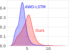
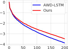
Density	Log Eigenvalues	Perplexity
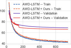
(a) L2 Distance	(b) Index	(c) Epochs (Wiki2)

Figure 1: (a) Kernel density estimation of the Euclidean distance to the nearest neighbor for each word; (b) Logarithmic scale singular values of embedding matrix. We normalize the singular values of each matrix so that the largest one is 1; (c) Training and validation perplexities vs. training epochs for AWD-LSTM (Merity et al., 2018a) and our approach on the Wikitext-2(WT2) datasets. We follow the training settings reported in Merity et al. (2018a). The kink in the middle represents the start of fine-tuning.

4 Related Works and Discussions

Adversarial training

Adversarial machine learning has been an active research area recently (Szegedy et al., 2013; Goodfellow et al., 2015; Athalye et al., 2018), in which algorithms are developed to either attack existing models by constructing adversarial examples, or train robust models to defend adversarial attacks. More related to our work, (Sankaranarayanan et al., 2018) proposes a layer-wise adversarial training method to regularize deep neural networks. In statistics learning and robust statistics, various adversarial-like ideas are also leveraged to construct efficient and robust estimators, mostly for preventing model specification or data corruption (e.g., Maronna et al., 2018; Duchi et al., 2016). Compared to these works, our work leverages the adversarial idea as a regularization technique specifically for neural language models and focuses on introducing adversarial noise only on the softmax layers, so that a simple closed form solution can be obtained.

Direct Diversity Regularization

There has been a body of literature on increasing the robustness by directly adding various forms of diversity-enforcing penalty functions (e.g., Elsayed et al., 2018; Xie et al., 2017; Liu et al., 2016, 2017; Chen et al., 2017; Wang et al., 2018). In the particular setting of enforcing diversity of word embeddings, Gao et al. (2019) show that adding a cosine similarity regularizer improves language modeling performance, which has the form $\sum_{i=1}^{|{\mathcal{V}}|}\sum_{j\neq i}^{|{\mathcal{V}}|}\frac{w_{i}^{\top}w_{j}}{||w_{i}||~{}||w_{j}||}.$ However, in language modeling, one disadvantage of the direct diversity regularization approach is that the vocabulary size $|{\mathcal{V}}|$ can be huge, and calculating the summation term exactly at each step is not feasible, while approximation with mini-batch samples may make it ineffective. Our method promotes diversity implicitly with theoretical guarantees and does not introduce computational overhead.

Large-margin classification

In a general sense, our method can be seen as an instance of constructing large-margin classifiers by enforcing the distance of a word to its neighbors larger than a margin if it’s recognized by any context. Learning large-margin classifiers has been extensively studied in the literature; see e.g., Weston et al. (1999); Tsochantaridis et al. (2005); Jiang et al. (2018); Elsayed et al. (2018); Liu et al. (2016, 2017).

Other Regularization Techniques for Language Models

Various other techniques have been also developed to address overfitting in RNN language models. For example, Gal & Ghahramani (2016) propose to use variational inference-based dropout (Srivastava et al., 2014) on recurrent neural networks, in which the same dropout mask is repeated at each time step for inputs, outputs, and recurrent layers for regularizing RNN models. Merity et al. (2018a) suggest to use DropConnect (Wan et al., 2013) on the recurrent weight matrices and report a series of encouraging benchmark results. Other types of regularization include activation regularization (Merity et al., 2017a), layer normalization (Ba et al., 2016), and frequency agnostic training (Gong et al., 2018), etc. Our work is orthogonal to these regularization and optimization techniques and can be easily combined with them to achieve further improvements, as we demonstrate in our experiments.

5 Empirical Results

We demonstrate the effectiveness of our method in two applications: neural language modeling and neural machine translation, and compare them with state-of-the-art architectures and learning methods. All models are trained with the weight-tying trick (Press & Wolf, 2016; Inan et al., 2017). Our code is available at:  https://github.com/ChengyueGongR/advsoft.

Method	Params	Valid	Test
Variational LSTM (Gal & Ghahramani, 2016)	19M	-	73.4
Variational LSTM + weight tying (Inan et al., 2017)	51M	71.1	68.5
NAS-RNN (Zoph & Le, 2017)	54M	-	62.4
DARTS (Liu et al., 2018a)	23M	58.3	56.1
w/o dynamic evaluation
AWD-LSTM  (Merity et al., 2018a)	24M	60.00	57.30
AWD-LSTM + Ours	24M	57.15	55.01
AWD-LSTM + MoS (Yang et al., 2018)	22M	56.54	54.44
AWD-LSTM + MoS + Ours	22M	54.98	52.87
AWD-LSTM + MoS + Partial Shuffled (Press, 2019)	22M	55.89	53.92
AWD-LSTM + MoS + Partial Shuffled + Ours	22M	54.10	52.20
+  dynamic evaluation (Krause et al., 2018)
AWD-LSTM  (Merity et al., 2018a)	24M	51.60	51.10
AWD-LSTM +Ours	24M	49.31	48.72
AWD-LSTM + MoS (Yang et al., 2018)	22M	48.33	47.69
AWD-LSTM + MoS + Ours	22M	47.15	46.52
AWD-LSTM + MoS + Partial Shuffled (Press, 2019)	22M	47.93	47.49
AWD-LSTM + MoS + Partial Shuffled + Ours	22M	46.63	46.01

Table 1: Perplexities on the validation and test sets on the Penn Treebank dataset. Smaller perplexities refer to better language modeling performance. Params denotes the number of model parameters.

Method	Params	Valid	Test
Variational LSTM (Inan et al., 2017) (h = 650)	28M	92.3	87.7
Variational LSTM (Inan et al., 2017) (h = 650) + weight tying	28M	91.5	87.0
1-layer LSTM (Mandt et al., 2017)	24M	69.3	65.9
2-layer skip connection LSTM  (Mandt et al., 2017) (tied)	24M	69.1	65.9
DARTS (Liu et al., 2018a)	33M	69.5	66.9
w/o dynamic evaluation
AWD-LSTM  (Merity et al., 2018a)	33M	68.60	65.80
AWD-LSTM + Ours	33M	64.01	61.56
AWD-LSTM + MoS (Yang et al., 2018)	35M	63.88	61.45
AWD-LSTM + MoS + Ours	35M	61.93	59.62
AWD-LSTM + MoS + Partial Shuffled (Press, 2019)	35M	62.38	59.98
AWD-LSTM + MoS + Partial Shuffled + Ours	35M	61.10	58.95
+  dynamic evaluation (Krause et al., 2018)
AWD-LSTM  (Merity et al., 2018a)	33M	46.40	44.30
AWD-LSTM + Ours	33M	42.48	40.71
AWD-LSTM + MoS (Yang et al., 2018)	35M	42.41	40.68
AWD-LSTM + MoS + Ours	35M	40.27	38.65
AWD-LSTM + MoS + Partial Shuffled (Press, 2019)	35M	40.75	39.03
AWD-LSTM + MoS + Partial Shuffled + Ours	35M	39.58	38.07

Table 2: Perplexities on validation and test sets on the Wikitext-2 dataset.

Method	Valid	Test
LSTM (Grave et al., 2017)	-	48.7
Temporal CNN (Bai et al., 2018)	-	45.2
GCNN (Dauphin et al., 2016)	-	37.2
LSTM + Hebbian (Rae et al., 2018)	34.1	34.3
4 layer QRNN (Merity et al., 2018b)	32.0	33.0
4 layer QRNN + Ours	30.6	31.6
+  post process (Rae et al., 2018)
LSTM + Hebbian + Cache + MbPA (Rae et al., 2018)	29.0	29.2
4 layer QRNN + Ours + dynamic evaluation	27.2	28.0

Table 3: Perplexities on validation and test sets on the Wikitext-103 dataset.

5.1 Experiments on Language Modeling

We test our method on three benchmark datasets: Penn Treebank (PTB), Wikitext-2 (WT2) and Wikitext-103 (WT103).

PTB

The PTB corpus (Marcus et al., 1993) has been a standard dataset used for benchmarking language models. It consists of 923k training, 73k validation and 82k test words. We use the processed version provided by Mikolov et al. (2010) that is widely used for this dataset (e.g., Merity et al., 2018a; Yang et al., 2018; Kanai et al., 2018; Gong et al., 2019).

WT2 and WT103

The WT2 and WT103 datasets are introduced in Merity et al. (2017b) as an alternative to the PTB dataset, and which contain lightly pre-possessed Wikipedia articles. The WT2 and WT103 contain approximately 2 million and 103 million words, respectively.

Experimental settings

For the PTB and WT2 datasets, we closely follow the regularization and optimization techniques introduced in AWD-LSTM (Merity et al., 2018a), which stacks a three-layer LSTM and performs optimization with a bag of tricks.

The WT103 corpus contains around 103 million tokens, which is significantly larger than the PTB and WT2 datasets. In this case, we use Quasi-Recurrent neural networks (QRNN)-based language models (Merity et al., 2018b; Bradbury et al., 2017) as our base model for efficiency. QRNN allows for parallel computation across both time-step and minibatch dimensions, enabling high throughput and good scaling for long sequences and large datasets.

Yang et al. (2018) show that softmax-based language models yield low-rank approximations and do not have enough capacity to model complex natural language. They propose a mixture of softmax (MoS) to break the softmax bottleneck and achieve significant improvements. We also evaluated our method within the MoS framework by directly following the experimental settings in Yang et al. (2018), except we replace the original softmax function with our adversarial softmax function.

The training procedure of AWD-LSTM-based language models can be decoupled into two stages: 1) optimizing the model with SGD and averaged SGD (ASGD); 2) restarting ASGD for fine-tuning. We report the perplexity scores at the end of both stages. We also report the perplexity scores with a recent proposed post-process method, dynamical evaluation (Krause et al., 2018) after fine-tuning.

Applying Adversarial MLE training

To investigate the effectiveness of our approach, we simply replace the softmax layer of baseline methods with our adversarial softmax function, with all other the parameters and architectures untouched. We empirically found that adding small annealed Gaussian noise in the input embedding layer makes our noisy model converge more quickly. We experimented with different ways of scaling the Gaussian dropout level and found that a small Gaussian noise with zero mean and a small variance, such that it decreases from 0.2 to 0.0 over the duration of the run, works well for all the tasks.

Note the optimal adversarial noise $\delta_{i}=-\epsilon h/||h||$ (see Algorithm 1) given RNN prediction $h$ associated with a target word $w_{i}$. Here, $\epsilon$ controls the magnitude of of the noise level. When $\epsilon=0$, our approach reduces to the original MLE training. We propose setting the noise level adaptive that proportional to the L2 norm of the target word embeddings, namely, by setting $\epsilon=\alpha||w_{i}||$ with $\alpha$ as a hyperparameter.

Figure 2 shows the training and validation perplexities on the PTB dataset with different choices of $\alpha$. We find that $\alpha$ in the range of $[0.001,0.01]$ perform similarly well. Larger values (e.g., $\alpha=0.05$) causes more difficult optimization and hence underfitting, while smaller values (e.g., $\alpha=0$ (the baseline approach)) tends to overfit as we observe from standard MLE training. We set $\alpha=0.005$ for the rest of experiments unless otherwise specified.

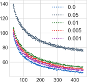
Training Perplexity	Validation Perplexity
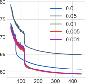
Epochs	Epochs

Figure 2: Training and validation perplexities on the PTB dataset with different choices of adversarial perturbation magnitude.

Results on PTB and WT2

The results on the PTB and WT2 corpus are illustrated in Tables 1 and 2, respectively. Methods with our adversarial softmax outperform the baselines in all settings. Our results establish a new single model state-of-the-art on PTB and WT2, achieving perplexity scores of 46.01 and 38.07, respectively. Specifically, our approach significantly improves AWD-LSTM by a margin of 2.29/2.38 and 3.92/3.59 in validation and test perplexity on the PTB and WT2 dataset. We also improve the AWD-LSTM-MoS baseline by an amount of 1.18/1.17 and 2.14/2.03 in perplexity for both datasets.

Results on WT103

Table 3 shows that on the large-scale WT103 dataset, we improve the QRNN baseline with 1.4/1.4 points in perplexity on validation and test sets, respectively. With dynamic evaluation, our method can achieve a test perplexity of 28.0, which is, to the authors’ knowledge, better than all existing CNN- or RNN-based models with similar numbers of model parameters.

Analysis

We further analyze the properties of the learned word embeddings on the WT2 dataset. Figure 1 (a) shows the distribution (via kernel density estimation) of the L2 distance between each word and its nearest neighbor learned by our method and the baseline, which verifies the diversity promoting property of our method. Figure 1 (b) shows the singular values of word embedding matrix learned by our model and that by the baseline model. We can see that, when trained with our method, the singular values distribute more uniformly, an indication that our embedding vectors fills a higher dimensional subspace.

Figure 1 (c) shows the training and validation perplexities of our method and baseline on AWD-LSTM. We can see that our method is less prone to overfitting. While the baseline model reaches a smaller training error quickly, our method has a larger training error at the same stage because it optimizes a more difficult adversarial objective, yet yields a significantly lower validation error.

5.2 Experiments on Machine Translation

We apply our method on machine translation tasks. Neural machine translation aims at building a single neural network that maximize translation performance. Given a source sentence $s$, translation is equivalent to finding a target sentence $t$ by maximizing the conditional probability $p(t|s)$. Here, we fit a parametrized model to maximize the conditional probability using a parallel training corpus. Specifically, we use an RNN encoder-decoder framework (Cho et al., 2014; Gehring et al., 2017b; Vaswani et al., 2017), upon which we apply our adversarial MLE training that learns to translate.

Datasets

We evaluate the proposed method on two translation tasks: WMT2014 English $\to$ German (En$\to$De) and IWSLT2014 German $\to$ English (De$\to$En) translation. We use the parallel corpora publicly available at WMT 2014 and IWSLT 2014, which have been widely used for benchmark neural machine translation tasks (Vaswani et al., 2017; Gehring et al., 2017b). For fair comparison, we follow the standard data pre-processing procedures described in Ranzato et al. (2016); Bahdanau et al. (2017).

WMT2014 En$\to$De We use the original training set for model training, which consists of 4.5 million sentence pairs. Source and target sentences are encoded by 37K shared sub-word tokens based on byte-pair encoding (BPE) (Sennrich et al., 2016b). We use the concatenation of newstest2012 and newstest2013 as the validation set and test on newstest2014.

IWSLT2014 De$\to$En This dataset contains 160K training sequences pairs and 7K validation sentence pairs. Sentences are encoded using BPE with a shared vocabulary of about 33K tokens. We use the concatenation of dev2010, tst2010, tst2011 and tst2011 as the test set, which is widely used in prior works (Bahdanau et al., 2017).

Experimental settings

We choose the Transformer-based state-of-the-art machine translation model  (Vaswani et al., 2017) as our base model and use Tensor2Tensor (Vaswani et al., 2018)  for implementation. Specifically, to be consistent with prior works, we closely follow the settings reported in Vaswani et al. (2017). We use the Adam optimizer (Kingma & Ba, 2014) and follow the learning rate warm-up strategy in Vaswani et al. (2017). Sentences are pre-processed using byte-pair encoding (Sennrich et al., 2016a) into subword tokens before training, and we measure the final performance with the BLEU score.

For the WMT2014 De$\to$En task, we evaluate on the Transformer-Base and Transformer-Big architectures, which consist of a 6-layer encoder and a 6-layer decoder with 512-dimensional and 1024-dimensional hidden units per layer, respectively. For the IWSLT2014 De$\to$En task, we evaluate on two standard configurations: Transformer-Small and Transformer-Base. For Transformer-Small, we stack a 4-layer encoder and a 4-layer decoder with 256-dimensional hidden units per layer. For Transformer-Base, we set the batch size to 6400 and the dropout rate to 0.4 following Wang et al. (2019). For both tasks, we share the BPE subword vocabulary for decoder and encoder.

Results

From Table 4 and Table 5, we can see that our method improves over the baseline algorithms for all settings. On the WMT2014 De$\to$En translation task, our method reaches 28.43 and 29.52 in BLEU score with the Transformer Base and Transformer Big architectures, respectively; this yields an 1.13/1.12 improvement over their corresponding baseline models. On the IWSLT2014 De$\to$En dataset, our method improves the BLEU score from 32.47 to 33.61 and 34.43 to 35.18 for the Transformer-Small and Transformer-Base configurations, respectively.

Method	BLEU
Local Attention (Luong et al., 2015)	20.90
ByteNet (Kalchbrenner et al., 2016)	23.75
ConvS2S (Gehring et al., 2017b)	25.16
Transformer Base  (Vaswani et al., 2017)	27.30
Transformer Base + Ours	28.43
Transformer Big  (Vaswani et al., 2017)	28.40
Transformer Big +  (Gao et al., 2019)	28.94
Transformer Big + Ours	29.52

Table 4: BLEU scores on the WMT2014 Ee$\to$De machine translation task.

Method	BLEU
Actor-critic (Bahdanau et al., 2017)	28.53
CNN-a (Gehring et al., 2017a)	30.04
Transformer Small (Vaswani et al., 2017)	32.47
Transformer Small + Ours	33.61
Transformer Base + (Wang et al., 2019)	34.43
Transformer Base + Ours	35.18

Table 5: BLEU scores on the IWSLT2014 De$\to$En machine translation task.

6 Conclusion

In this work, we present an adversarial MLE training strategy for neural language modeling, which promotes diversity in the embedding space and improves the generalization performance. Our approach can be easily used as a drop-in replacement for standard MLE-based model with no additional training parameters and computational overhead. Applying this approach to a variety of language modeling and machine translation tasks, we achieve improvements over state-of-the-art baseline models on standard benchmarks.

References

- Anderson et al. (2018) Peter Anderson, Xiaodong He, Chris Buehler, Damien Teney, Mark Johnson, Stephen Gould, and Lei Zhang. Bottom-up and top-down attention for image captioning and visual question answering. In CVPR, volume 3, pp. 6, 2018.
- Athalye et al. (2018) Anish Athalye, Nicholas Carlini, and David Wagner. Obfuscated gradients give a false sense of security: Circumventing defenses to adversarial examples. Proceedings of the 35th International Conference on Machine Learning, ICML, 2018.
- Ba et al. (2016) Jimmy Lei Ba, Jamie Ryan Kiros, and Geoffrey E Hinton. Layer normalization. arXiv preprint arXiv:1607.06450, 2016.
- Bahdanau et al. (2017) Dzmitry Bahdanau, Philemon Brakel, Kelvin Xu, Anirudh Goyal, Ryan Lowe, Joelle Pineau, Aaron Courville, and Yoshua Bengio. An actor-critic algorithm for sequence prediction. International Conference on Learning Representations, ICLR, 2017.
- Bai et al. (2018) Shaojie Bai, J. Zico Kolter, and Vladlen Koltun. Convolutional sequence modeling revisited, 2018. URL https://openreview.net/forum?id=rk8wKk-R-.
- Bradbury et al. (2017) James Bradbury, Stephen Merity, Caiming Xiong, and Richard Socher. Quasi-recurrent neural networks. International Conference on Learning Representations, ICLR, 2017.
- Chen et al. (2017) Binghui Chen, Weihong Deng, and Junping Du. Noisy softmax: Improving the generalization ability of dcnn via postponing the early softmax saturation. In The IEEE Conference on Computer Vision and Pattern Recognition, CVPR, 2017.
- Cho et al. (2014) Kyunghyun Cho, Bart Van Merriënboer, Caglar Gulcehre, Dzmitry Bahdanau, Fethi Bougares, Holger Schwenk, and Yoshua Bengio. Learning phrase representations using rnn encoder-decoder for statistical machine translation. Conference on Empirical Methods in Natural Language Processing, EMNLP,, 2014.
- Chung et al. (2014) Junyoung Chung, Caglar Gulcehre, KyungHyun Cho, and Yoshua Bengio. Empirical evaluation of gated recurrent neural networks on sequence modeling. arXiv preprint arXiv:1412.3555, 2014.
- Cogswell et al. (2016) Michael Cogswell, Faruk Ahmed, Ross Girshick, Larry Zitnick, and Dhruv Batra. Reducing overfitting in deep networks by decorrelating representations. ICLR, 2016.
- Cortes & Vapnik (1995) Corinna Cortes and Vladimir Vapnik. Support-vector networks. Machine learning, 20(3):273–297, 1995.
- Dauphin et al. (2016) Yann N Dauphin, Angela Fan, Michael Auli, and David Grangier. Language modeling with gated convolutional networks. arXiv preprint arXiv:1612.08083, 2016.
- Duchi et al. (2016) John Duchi, Peter Glynn, and Hongseok Namkoong. Statistics of robust optimization: A generalized empirical likelihood approach. arXiv preprint arXiv:1610.03425, 2016.
- Elsayed et al. (2018) Gamaleldin F Elsayed, Dilip Krishnan, Hossein Mobahi, Kevin Regan, and Samy Bengio. Large margin deep networks for classification. in Advances in Neural Information Processing Systems, 2018.
- Gal & Ghahramani (2016) Yarin Gal and Zoubin Ghahramani. A theoretically grounded application of dropout in recurrent neural networks. In Advances in neural information processing systems, pp. 1019–1027, 2016.
- Gao et al. (2019) Jun Gao, Di He, Xu Tan, Tao Qin, Liwei Wang, and Tieyan Liu. Representation degeneration problem in training natural language generation models. ICLR, 2019.
- Gehring et al. (2017a) Jonas Gehring, Michael Auli, David Grangier, and Yann N Dauphin. A convolutional encoder model for neural machine translation. ACL, 2017a.
- Gehring et al. (2017b) Jonas Gehring, Michael Auli, David Grangier, Denis Yarats, and Yann N Dauphin. Convolutional sequence to sequence learning. ICML, 2017b.
- Gong et al. (2018) Chengyue Gong, Di He, Xu Tan, Tao Qin, Liwei Wang, and Tie-Yan Liu. Frage: frequency-agnostic word representation. In Advances in Neural Information Processing Systems, pp. 1339–1350, 2018.
- Gong et al. (2019) Chengyue Gong, Xu Tan, Di He, and Tao Qin. Sentence-wise smooth regularization for sequence to sequence learning. AAAI, 2019.
- Goodfellow et al. (2015) Ian Goodfellow, Jonathon Shlens, and Christian Szegedy. Explaining and harnessing adversarial examples. In International Conference on Learning Representations, 2015.
- Grave et al. (2017) Edouard Grave, Armand Joulin, Moustapha Cissé, David Grangier, and Hervé Jégou. Efficient softmax approximation for gpus. International Conference on Machine Learning, ICML, 2017.
- Hochreiter & Schmidhuber (1997) Sepp Hochreiter and Jürgen Schmidhuber. Long short-term memory. Neural computation, 9(8):1735–1780, 1997.
- Inan et al. (2017) Hakan Inan, Khashayar Khosravi, and Richard Socher. Tying word vectors and word classifiers: A loss framework for language modeling. ICLR, 2017.
- Jiang et al. (2018) Yiding Jiang, Dilip Krishnan, Hossein Mobahi, and Samy Bengio. Predicting the generalization gap in deep networks with margin distributions. arXiv preprint arXiv:1810.00113, 2018.
- Kalchbrenner et al. (2016) Nal Kalchbrenner, Lasse Espeholt, Karen Simonyan, Aaron van den Oord, Alex Graves, and Koray Kavukcuoglu. Neural machine translation in linear time. arXiv preprint arXiv:1610.10099, 2016.
- Kanai et al. (2018) Sekitoshi Kanai, Yasuhiro Fujiwara, Yuki Yamanaka, and Shuichi Adachi. Sigsoftmax: Reanalysis of the softmax bottleneck. In Advances in Neural Information Processing Systems, 2018.
- Khodak et al. (2018) Mikhail Khodak, Nikunj Saunshi, Yingyu Liang, Tengyu Ma, Brandon Stewart, and Sanjeev Arora. A la carte embedding: Cheap but effective induction of semantic feature vectors. ACL, 2018.
- Kingma & Ba (2014) Diederik P Kingma and Jimmy Ba. Adam: A method for stochastic optimization. arXiv preprint arXiv:1412.6980, 2014.
- Koehn (2009) Philipp Koehn. Statistical machine translation. Cambridge University Press, 2009.
- Krause et al. (2018) Ben Krause, Emmanuel Kahembwe, Iain Murray, and Steve Renals. Dynamic evaluation of neural sequence models. ICML, 2018.
- Liu et al. (2018a) Hanxiao Liu, Karen Simonyan, and Yiming Yang. Darts: Differentiable architecture search. arXiv preprint arXiv:1806.09055, 2018a.
- Liu et al. (2016) Weiyang Liu, Yandong Wen, Zhiding Yu, and Meng Yang. Large-margin softmax loss for convolutional neural networks. In ICML, pp. 507–516, 2016.
- Liu et al. (2017) Weiyang Liu, Yandong Wen, Zhiding Yu, Ming Li, Bhiksha Raj, and Le Song. Sphereface: Deep hypersphere embedding for face recognition. In The IEEE Conference on Computer Vision and Pattern Recognition (CVPR), volume 1, pp. 1, 2017.
- Liu et al. (2018b) Weiyang Liu, Rongmei Lin, Zhen Liu, Lixin Liu, Zhiding Yu, Bo Dai, and Le Song. Learning towards minimum hyperspherical energy. NeurIPS, 2018b.
- Luong et al. (2015) Minh-Thang Luong, Hieu Pham, and Christopher D Manning. Effective approaches to attention-based neural machine translation. Proceedings of the 2015 Conference on Empirical Methods in Natural Language Processing, 2015.
- Mandt et al. (2017) Stephan Mandt, Matthew D Hoffman, and David M Blei. Stochastic gradient descent as approximate Bayesian inference. The Journal of Machine Learning Research, 2017.
- Marcus et al. (1993) Mitchell P Marcus, Mary Ann Marcinkiewicz, and Beatrice Santorini. Building a large annotated corpus of english: The penn treebank. Computational linguistics, 19(2):313–330, 1993.
- Maronna et al. (2018) Ricardo A Maronna, R Douglas Martin, Victor J Yohai, and Matías Salibián-Barrera. Robust statistics: theory and methods (with R). Wiley, 2018.
- Merity et al. (2017a) Stephen Merity, Bryan McCann, and Richard Socher. Revisiting activation regularization for language rnns. ICML, 2017a.
- Merity et al. (2017b) Stephen Merity, Caiming Xiong, James Bradbury, and Richard Socher. Pointer sentinel mixture models. ICLR, 2017b.
- Merity et al. (2018a) Stephen Merity, Nitish Shirish Keskar, and Richard Socher. Regularizing and optimizing lstm language models. ICLR, 2018a.
- Merity et al. (2018b) Stephen Merity, Nitish Shirish Keskar, and Richard Socher. An analysis of neural language modeling at multiple scales. arXiv preprint arXiv:1803.08240, 2018b.
- Mikolov et al. (2010) Tomáš Mikolov, Martin Karafiát, Lukáš Burget, Jan Černockỳ, and Sanjeev Khudanpur. Recurrent neural network based language model. In Eleventh Annual Conference of the International Speech Communication Association, 2010.
- Mu et al. (2018) Jiaqi Mu, Suma Bhat, and Pramod Viswanath. All-but-the-top: Simple and effective postprocessing for word representations. ICLR, 2018.
- Press (2019) Ofir Press. Partially shuffling the training data to improve language models. arXiv preprint arXiv:1903.04167, 2019.
- Press & Wolf (2016) Ofir Press and Lior Wolf. Using the output embedding to improve language models. Proceedings of the 15th Conference of the European Chapter of the Association for Computational Linguistics: Volume 2, Short Papers, 2016.
- Rae et al. (2018) Jack W Rae, Chris Dyer, Peter Dayan, and Timothy P Lillicrap. Fast parametric learning with activation memorization. ICML, 2018.
- Ranzato et al. (2016) Marc’Aurelio Ranzato, Sumit Chopra, Michael Auli, and Wojciech Zaremba. Sequence level training with recurrent neural networks. ICLR, 2016.
- Sankaranarayanan et al. (2018) Swami Sankaranarayanan, Arpit Jain, Rama Chellappa, and Ser Nam Lim. Regularizing deep networks using efficient layerwise adversarial training. In Thirty-Second AAAI Conference on Artificial Intelligence, 2018.
- Sennrich et al. (2016a) Rico Sennrich, Barry Haddow, and Alexandra Birch. Neural machine translation of rare words with subword units. In ACL, 2016a.
- Sennrich et al. (2016b) Rico Sennrich, Barry Haddow, and Alexandra Birch. Neural machine translation of rare words with subword units. Proceedings of the 54th Annual Meeting of the Association for Computational Linguistics (Volume 1: Long Papers), 2016b.
- Srivastava et al. (2014) Nitish Srivastava, Geoffrey Hinton, Alex Krizhevsky, Ilya Sutskever, and Ruslan Salakhutdinov. Dropout: a simple way to prevent neural networks from overfitting. The Journal of Machine Learning Research, 15(1):1929–1958, 2014.
- Szegedy et al. (2013) Christian Szegedy, Wojciech Zaremba, Ilya Sutskever, Joan Bruna, Dumitru Erhan, Ian Goodfellow, and Rob Fergus. Intriguing properties of neural networks. arXiv preprint arXiv:1312.6199, 2013.
- Tsochantaridis et al. (2005) Ioannis Tsochantaridis, Thorsten Joachims, Thomas Hofmann, and Yasemin Altun. Large margin methods for structured and interdependent output variables. Journal of machine learning research, 6(Sep):1453–1484, 2005.
- Vaswani et al. (2017) Ashish Vaswani, Noam Shazeer, Niki Parmar, Jakob Uszkoreit, Llion Jones, Aidan N Gomez, Łukasz Kaiser, and Illia Polosukhin. Attention is all you need. In Advances in Neural Information Processing Systems, pp. 6000–6010, 2017.
- Vaswani et al. (2018) Ashish Vaswani, Samy Bengio, Eugene Brevdo, Francois Chollet, Aidan N. Gomez, Stephan Gouws, Llion Jones, Łukasz Kaiser, Nal Kalchbrenner, Niki Parmar, Ryan Sepassi, Noam Shazeer, and Jakob Uszkoreit. Tensor2tensor for neural machine translation. CoRR, abs/1803.07416, 2018. URL http://arxiv.org/abs/1803.07416.
- Wan et al. (2013) Li Wan, Matthew Zeiler, Sixin Zhang, Yann Le Cun, and Rob Fergus. Regularization of neural networks using dropconnect. In International Conference on Machine Learning, pp. 1058–1066, 2013.
- Wang et al. (2018) Feng Wang, Jian Cheng, Weiyang Liu, and Haijun Liu. Additive margin softmax for face verification. IEEE Signal Processing Letters, 25(7):926–930, 2018.
- Wang et al. (2019) Yiren Wang, Yingce Xia, Tianyu He, Fei Tian, Tao Qin, ChengXiang Zhai, and Tie-Yan Liu. Multi-agent dual learning. In International Conference on Learning Representations, 2019.
- Weston et al. (1999) Jason Weston, Chris Watkins, et al. Support vector machines for multi-class pattern recognition. In Esann, volume 99, pp. 219–224, 1999.
- Xie et al. (2017) Bo Xie, Yingyu Liang, and Le Song. Diverse neural network learns true target functions. Artificial Intelligence and Statistics, 2017.
- Xu et al. (2015) Kelvin Xu, Jimmy Ba, Ryan Kiros, Kyunghyun Cho, Aaron Courville, Ruslan Salakhudinov, Rich Zemel, and Yoshua Bengio. Show, attend and tell: Neural image caption generation with visual attention. In International conference on machine learning, pp. 2048–2057, 2015.
- Yang et al. (2018) Zhilin Yang, Zihang Dai, Ruslan Salakhutdinov, and William W Cohen. Breaking the softmax bottleneck: A high-rank rnn language model. ICLR, 2018.
- Yu & Deng (2016) Dong Yu and Li Deng. AUTOMATIC SPEECH RECOGNITION. Springer, 2016.
- Zoph & Le (2017) Barret Zoph and Quoc V Le. Neural architecture search with reinforcement learning. ICLR, 2017.