On Regularization of Convolutional Kernels in Neural Networks

Abstract

Convolutional neural network is an important model in deep learning. To avoid exploding/vanishing gradient problems and to improve the generalizability of a neural network, it is desirable to have a convolution operation that nearly preserves the norm, or to have the singular values of the transformation matrix corresponding to a convolutional kernel bounded around $1$. We propose a penalty function that can be used in the optimization of a convolutional neural network to constrain the singular values of the transformation matrix around $1$. We derive an algorithm to carry out the gradient descent minimization of this penalty function in terms of convolution kernels. Numerical examples are presented to demonstrate the effectiveness of the method.

Keywords: penalty function, transformation matrix, convolutional layers, generalizability, unstable gradient.

1 Introduction

The classical convolution operation is an essential tool in signal processing. More general forms of convolution that use no flip in multiplications but may have different strides and padding patterns have been introduced and widely used in deep learning [7]. Here, only element-wise multiplication and addition are performed and there is no reverse multiplication with the convolutional kernel. Without loss of generality, we will consider in this paper 2-dimensional convolutions with unit strides and with zero padding. Specifically, given a convolutional kernel matrix $K=[k_{ij}]\in\mathbb{R}^{k\times k}$ and an input matrix $X=[x_{ij}]\in\mathbb{R}^{N\times N}$, we consider the convolution of $K$ and $X$, denoted by $Y=K*X\in\mathbb{R}^{N\times N}$, as defined by

$$y_{r,s}=(K*X)_{r,s}=\sum_{p\in\{1,\cdots,k\}}\sum_{q\in\{1,\cdots,k\}}x_{r-m+p,s-m+q}k_{p,q},$$ (1.1)

where $m=\ulcorner k/2\urcorner$, and $x_{i,j}=0$ if $i\leq 0$ or $i>N$, or $j\leq 0$ or $j>N$. Here and throughout, $\ulcorner x\urcorner$ denotes the smallest integer greater than or equal to $x$.

Indeed, in convolutional neural networks (CNNs), a more general form of convolution is typically used where the input is a multichannel signal represented by a 3-dimensional tensor $X=[x_{ijk}]\in\mathbb{R}^{N\times N\times g}$. Namely, the input $X$ has $g$ channels of $N\times N$ matrices. Then, a convolutional kernel is represented by a 4-dimensional tensor $K=[k_{ijk\ell}]\in\mathbb{R}^{k\times k\times g\times h}$ and the multichannel convolution of $K$ and $X$ produces a 3 dimensional tensor output $Y=[y_{ijk}]\in\mathbb{R}^{N\times N\times h}$, as denoted by $Y=K*X$ and defined by

$$y_{r,s,c}=(K*X)_{r,s,c}=\sum_{d\in\{1,\cdots,g\}}\sum_{p\in\{1,\cdots,k\}}\sum_{q\in\{1,\cdots,k\}}x_{r-m+p,s-m+q,d}k_{p,q,d,c},$$ (1.2)

where $m=\ulcorner k/2\urcorner$ and $x_{i,j,d}=0$ if $i\leq 0$ or $i>N$, or $j\leq 0$ or $j>N$. We will also call (1.1) a one-channel convolution, which is a special case of the multichannel convolution (1.2).

Clearly, the convolution operation is a linear transformation on $X$ and each convolutional kernel corresponds to a linear transformation matrix. Indeed, the convolution equation $Y=K*X$ can be written as a matrix-vector product after reshaping $X$ and $Y$. Let $vec(X)$ denote the reshape of $X$ into a vector as follows. If $X$ is a matrix, $vec(X)$ is the column vector obtained by stacking the columns of $X$ on top of one another. If $X$ is a tensor, $vec(X)$ is the column vector obtained by stacking the columns of the flattening of $X$ along the first index (see [8] or Section 2.2 for more details). Then, given a kernel $K$, there is a corresponding matrix $M$ such that

$$vec(Y)=M\,vec(X).$$

In deep convolutional networks, a convolution kernel $K$ is a model parameter that defines the input and output $Y=K*X$ in a convolution layer and we need to construct $K$ by optimizing certain loss function ${\cal L}(K)$ with respect to $K$ (see Subsection 1.1 below). It is then desirable to construct $K$ such that

$$\|vec(Y)\|_{2}\approx\|vec(X)\|_{2}$$ (1.3)

Such properties ensure bounded gradients which is critical in training deep convolutional neural networks [11]. Ideally then, we would like to construct $K$ so that the corresponding $M$ has orthonormal columns (i.e. $M^{T}M=I$), but this is in general impossible because $M^{T}M=I$ involves $gN^{2}(gN^{2}+1)/2$ equations while $K$ has only $k^{2}gh$ parameters with $k\ll N$ usually in neural networks. One known situation where an orthogonal $M$ can be constructed is the one-channel periodic convolution with full sized $N\times N$ kernel (i.e. k=N), for which the convolution becomes a diagonal matrix multiplication after discrete Fourier transforms; see [18] for example. For a multichannel convolution with a small kernel ($k\ll N$), a more realistic goal is to construct a kernel so that the singular values of the corresponding transformation matrix $M$ are bounded around $1$.

In this paper, we focus on the numerical problem of constructing a convolutional kernel $K$ using a suitable regularization function to move the singular values of $M$ towards $1$. One may consider explicitly adding $max\{|\sigma_{max}(M)-1|,|\sigma_{min}(M)-1|\}$ to ${\cal L}(K)$ as a penalty function, where $\sigma_{max}(\cdot)$ and $\sigma_{min}(\cdot)$ denote the largest and respectively the smallest singular values of a matrix, but with two objectives, this is more difficult to implement however. We propose using ${\cal R}_{\alpha}(K):=\sigma_{max}(M^{T}M-\alpha I)$ (for some $\alpha>0$) as a penalty function for the regularization of the convolutional kernel. We will show that reducing ${\cal R}_{\alpha}(K)$ keeps the largest singular value bounded from above and the smallest singular value from below. Equivalently up to a scaling, this reduces the condition number of $M$. We will then derive a gradient descent algorithm for minimizing ${\cal R}_{\alpha}(K)$. Numerical examples will be presented to illustrate our method.

There have been many works devoted to enforcing the orthogonality or spectral norm regularization on the weights of a neural network; see [3, 6, 17, 24] and the references contained therein. For a convolutional layer, some of these works enforce the constraint directly on the $h\times(gkk)$ matrix reshaped from the kernel $K\in\mathbb{R}^{k\times k\times g\times h}$ without any clear impacts on $M$ [3, 6]. [17, 24] normalize a matrix reshaped from $K$ by its spectral norm. [18] first constructs a full-sized kernel under the periodic convolution that has a corresponding $M$ with bounded singular values and then projects the full-sized convolutional kernel to a desirable small one. This projection obviously may not preserve the desirable singular value bound of the original kernel. Compared with those approaches, our method works on the convolution kernel $K$ but regularize on the singular values of $M$. We also note that there are many works on constructing orthogonal weight matrices in the context of recurrent neural networks; see [1, 10, 16, 22] and the references contained therein, but we are concerned here with optimizing the singular values of a linear transformation defined by a convolution kernel rather than a general weight matrix.

The rest of the paper is organized as follows. In subsection 1.1, we will discuss the origin of our problem in deep learning. In Section 2.1, we first propose the penalty function and discuss its theoretical property. We then derive the gradient formula and propose the gradient descent algorithm for the one-channel case in Subsection 2.1 and for the multichannel case in Subsection 2.2. In Section 3, we present numerical results to show the effectiveness of the method. We end in Section 4 with some concluding remarks.

1.1 Applications in deep learning

The regularization problem we consider arises in training of deep convolutional neural networks. Convolutional neural network is one of the most widely used model of deep learning. A typical convolutional neural network consists of convolutional layers, pooling layers, and fully connected layers. Training the neural networks is an optimization problem, which seeks optimal weights (parameters) by reaching the minimum of loss function on the training data. This can be described as follows: given a labeled data set $\{(X_{i},Y_{i})\}_{i=1}^{N}$, where $X_{i}$ is the input and $Y_{i}$ is the output, and a given parametric family of functions $\mathbb{F}=\{f(\Theta,X)\}$, where $\Theta$ denotes the parameters contained in the function, the goal of training the neural networks is to find the best parameters $\Theta$ such that $Y_{i}\approx f(\Theta,X_{i})$ for $i=1,\cdots,N$. The practice is to minimize the so called loss function, e.g $\Sigma_{i=1}^{N}\|Y_{i}-f(\Theta,X_{i})\|_{2}^{2}$ on the training data set.

For example, a typical convolutional neural network has $l$ convolutional layers parameterized by $l$ convolution kernels $K_{p}$ ($1\leq p\leq l$) and $m$ so-called fully-connected layers defined by weight matrices $W_{q},(1\leq q\leq m)$; we omit the bias for the ease of notation. Then the output of the network can be written as $Y=f(K_{1},K_{2},\cdots,K_{l},W_{1},W_{2},\cdots,W_{m},X)$ and we train the network by solving the following optimization problem for the training dataset $\{(X_{i},Y_{i})\}_{i=1}^{N}$:

$$min_{K_{1},K_{2},\cdots,K_{l},W_{1},W_{2},\cdots,W_{m}}\frac{1}{N}\Sigma_{i=1}^{N}\|Y_{i}-f(K_{1},K_{2},\cdots,K_{l},W_{1},W_{2},\cdots,W_{m},X_{i})\|.$$ (1.4)

Exploding and vanishing gradients are fundamental obstacles to solving (1.4) or training of deep neural networks [11]. The singular values of the Jacobian of a layer bound the factor by which it changes the norm of the backpropagated signal. If these singular values are all close to $1$, then gradients neither explode nor vanish. This can also help improve the generalizability. Specifically, although the training of neural networks can be seen as an optimization problem, but the goal of training is not merely to minimize the loss function on training data set. In fact, the performance of the trained model on new data is the ultimate concern. That is to say, after we find the weights or parameters $\Theta$ through minimizing the loss function on training data set, we will use the weights $\Theta$ to get a neural network to predict the output or label for new input data. Generalizability, the ability of a network to extend its performance on the training data to new data, can be improved through reducing the sensitivity of the output against the input data perturbation [9, 20, 21, 23, 24]. This again can be achieved through (1.3) and hence through regularizing the singular values of $M$.

2 Regularization of Convolution Kernels

One way to achieve (1.3) is by minimizing $\sigma_{max}(M^{T}M-I)$ so that $M$ is close to being orthogonal. Since the number of parameters in the convolution kernel $K$ may be relatively small, the minimum value with respect to $K$ may not be very close to $0$. Namely, enforcing $M$ to be nearly orthogonal may be too strong a condition to satisfy. Note that our goal to decrease $\sigma_{max}(M)$ while increasing $\sigma_{min}(M)$ is equivalent, up to a scaling, to decreasing the condition number of $M$. In light of this, we propose to minimize ${\cal R}_{\alpha}(K):=\sigma_{max}(M^{T}M-\alpha I)$ for some fixed $\alpha$. The following theorem justifies this approach.

Theorem 2.1.

Let $\alpha>0$ and $M\in\mathbb{R}^{m\times n}$ be such that ${\cal R}_{\alpha}(K)=\sigma_{max}(M^{T}M-\alpha I)<t\alpha$ for some $0<t\leq 1$. Then the largest and the smallest singular value of $M$, denoted by $\sigma_{max}(M)$ and $\sigma_{min}(M)$ respectively, satisfy that

$$\sqrt{(1-t)\alpha}<\sigma_{min}(M)\leq\sigma_{max}(M)<\sqrt{(1+t)\alpha}.$$

In particular, $\kappa_{2}(M):=\frac{\sigma_{max}(M)}{\sigma_{min}(M)}<\sqrt{\frac{1+t}{1-t}}.$

Proof.

We use $\lambda_{1}(\cdot),\lambda_{2}(\cdot),\cdots,\lambda_{m}(\cdot)$ to denote all eigenvalues of an $m\times m$ matrix. Since $M^{T}M-\alpha I$ is symmetric and $\sigma_{max}(M^{T}M-\alpha I)<t\alpha$, then for all $i=1,2,\cdots,m$, we have

$$-t\alpha<\lambda_{i}(M^{T}M-\alpha I)<t\alpha,$$

and thus

$$(1-t)\alpha<\lambda_{i}(M^{T}M)<(1+t)\alpha.$$

Therefore we have

$$\sqrt{(1-t)\alpha}<\sigma_{min}(M)\leq\sigma_{max}(M)<\sqrt{(1+t)\alpha}.$$

The bound on the condition number $\kappa_{2}(M)$ follows immediately. ∎

Theorem 2.1 suggests that reducing ${\cal R}_{\alpha}(K)$ to a value less than $\alpha$ is sufficient to keep $\sigma_{max}(M)$ bounded above and $\sigma_{min}(M)$ bounded below. Then, the reduction in ${\cal R}_{\alpha}(K)$ needed to maintain boundedness of the singular values may be less by using a larger value of $\alpha$. We next discuss the gradient descent algorithm to minimize ${\cal R}_{\alpha}(K)$. We first discuss the one-channel convolution and then present the generalization to multichannel cases.

2.1 One-channel convolution

We first consider the one-channel convolution (1.1), i.e. in the context of (1.2), the numbers of input channels and the output channels are both $1$. In this case, the kernel is a $k\times k$ matrix and the input and the output are $N\times N$ matrices. For the ease of notation, we use a $3\times 3$ convolution kernel to illustrate the associated transformation matrix. Let the convolution kernel $K$ be

$$K=\left(\begin{array}[]{ccc}k_{11}&k_{12}&k_{13}\\ k_{21}&k_{22}&k_{23}\\ k_{31}&k_{32}&k_{33}\end{array}\right).$$

Then the transformation matrix corresponding to the convolution operation is

$$M=M(K):=\left(\begin{array}[]{cccccc}A_{0}&A_{-1}&0&0&\cdots&0\\ A_{1}&A_{0}&A_{-1}&\ddots&\ddots&\vdots\\ 0&A_{1}&A_{0}&\ddots&\ddots&0\\ 0&\ddots&\ddots&\ddots&A_{-1}&0\\ \vdots&\ddots&\ddots&A_{1}&A_{0}&A_{-1}\\ 0&\cdots&0&0&A_{1}&A_{0}\\ \end{array}\right)$$ (2.8)

where

$$A_{0}=\left(\begin{array}[]{cccccc}k_{22}&k_{23}&0&0&\cdots&0\\ k_{21}&k_{22}&k_{23}&\ddots&\ddots&\vdots\\ 0&k_{21}&k_{22}&\ddots&\ddots&0\\ 0&\ddots&\ddots&\ddots&k_{23}&0\\ \vdots&\ddots&\ddots&k_{21}&k_{22}&k_{23}\\ 0&\cdots&0&0&k_{21}&k_{22}\end{array}\right),\quad A_{-1}=\left(\begin{array}[]{cccccc}k_{32}&k_{33}&0&0&\cdots&0\\ k_{31}&k_{32}&k_{33}&\ddots&\ddots&\vdots\\ 0&k_{31}&k_{32}&\ddots&\ddots&0\\ 0&\ddots&\ddots&\ddots&k_{33}&0\\ \vdots&\ddots&\ddots&k_{31}&k_{32}&k_{33}\\ 0&\cdots&0&0&k_{31}&k_{32}\end{array}\right),$$

$$A_{1}=\left(\begin{array}[]{cccccc}k_{12}&k_{13}&0&0&\cdots&0\\ k_{11}&k_{12}&k_{13}&\ddots&\ddots&\vdots\\ 0&k_{11}&k_{12}&\ddots&\ddots&0\\ 0&\ddots&\ddots&\ddots&k_{13}&0\\ \vdots&\ddots&\ddots&k_{11}&k_{12}&k_{13}\\ 0&\cdots&0&0&k_{11}&k_{12}\end{array}\right).$$

In particular, $M$ is a $N^{2}\times N^{2}$ doubly block banded Toeplitz matrix, i.e., a block banded Toeplitz matrix with its blocks are banded Toeplitz matrices [12].

To minimize ${\cal R}_{\alpha}(K)=\sigma_{max}(M^{T}M-\alpha I)$, we derive a formula for its gradient with respect to $K$, i.e., $\partial\sigma_{max}(M^{T}M-I)/\partial k_{p,q}$ with $M=M(K)$ being the transformation matrix defined from $K$ in (2.8) for each entry $k_{p,q}$ of the convolution kernel. Our result provides a framework to use ${\cal R}_{\alpha}(K)$ as a regularization term in the optimization of ${\cal L}(K)$ in convolutional neural networks. To compute the gradient, we need the following classical result on the first order perturbation expansion about a simple singular value; see [19].

Lemma 2.1.

Let $\sigma$ be a simple singular value of $A=[a_{ij}]\in\mathbb{R}^{m\times m}$ ($n\geq p$) with normalized left and right singular vectors $u$ and $v$. Then $\partial\sigma/\partial a_{ij}$ is $u(i)v(j)$, where $u(i)$ is the $i$-th entry of vector $u$ and $v(j)$ is the $j$-th entry of vector $v$.

For our situation, we need to consider perturbation of $M^{T}M$ when $M$ is changed. Clearly, if an entry $m_{ij}$ changes, only the entries belonging to $j$-th row or $j$-th volume of the matrix $M^{T}M$ are affected. Actually, we have the following lemma.

Lemma 2.2.

Let $M=[m_{ij}]\in\mathbb{R}^{m\times n}$ and let $\sigma_{max}(M^{T}M-\alpha I)$ be the largest singular value of $M^{T}M-\alpha I$ with $u$ and $v$ normalized left and right singular vectors. Assuming $\sigma_{max}(M^{T}M-\alpha I)$ is simple and positive, we have

$$\frac{\partial\sigma_{max}(M^{T}M-\alpha I)}{\partial m_{ij}}=v(j)u^{T}M^{T}e_{i}+u(j)e_{i}^{T}Mv$$ (2.11)

where $e_{k}$ denotes the $k$-th column of the $n\times n$ identity matrix.

Proof.

Let $A=[a_{ij}]=M^{T}M-\alpha I$. A direct calculation yields

$$\frac{\partial A}{\partial m_{ij}}=M^{T}\frac{\partial M}{\partial m_{ij}}+\frac{\partial(M^{T})}{\partial m_{ij}}M=M^{T}(e_{i}e_{j}^{T})+(e_{j}e_{i}^{T})M.$$

It follows from this, lemma 2.1 and the chain rule that

$$\frac{\partial\sigma_{max}(A)}{\partial m_{ij}} = \sum_{s=1}^{n}\sum_{t=1}^{n}\frac{\partial\sigma_{max}(A)}{\partial a_{s,t}}\frac{\partial a_{s,t}}{\partial m_{ij}}$$

$$= \sum_{s=1}^{n}\sum_{t=1}^{n}u(s)v(t)\frac{\partial a_{s,t}}{\partial m_{ij}}$$

$$= u^{T}\frac{\partial A}{\partial m_{ij}}v$$

$$= u^{T}(M^{T}(e_{i}e_{j}^{T})+(e_{j}e_{i}^{T})M)v$$

$$= v(j)u^{T}M^{T}e_{i}+u(j)e_{i}^{T}Mv$$

∎

We can now derive a formula for the gradient descent of $\sigma_{max}(M^{T}M-I)$ with respect to the convolution kernel $K$ as follows.

Theorem 2.2.

Assume the largest singular value of $M^{T}M-\alpha I$, denoted by $\sigma_{max}(M^{T}M-\alpha I)$, is simple and positive, where $M=[m_{ij}]=M(K)\in\mathbb{R}^{n\times n}$ is the doubly block banded Toeplitz matrix (2.8) corresponding to a one channel convolution kernel $K=[k_{ij}]\in\mathbb{R}^{k\times k}$. Assume $u$ and $v$ are normalized left and right singular vectors of $M^{T}M-\alpha I$ associated with $\sigma_{max}(M^{T}M-\alpha I)$. Given $(p,q)$, if $\Omega_{p,q}$ denotes the set of all indexes $(i,j)$ such that $m_{ij}=k_{p,q}$, we have

$$\frac{\partial\sigma_{max}(M^{T}M-\alpha I)}{\partial k_{p,q}}=\sum_{(i,j)\in\Omega_{p,q}}(\sum_{t=1}^{n}u(j)v(t)m_{it}+\sum_{s=1}^{n}u(s)v(j)m_{is}).$$ (2.12)

Proof.

From (2.8), $m_{ij}$ is either 0 or equal to some $k_{p,q}$. Indeed, $m_{ij}=k_{p,q}$ if and only if $(i,j)\in\Omega_{p,q}$. Now, applying the chain rule to calculate $\partial\sigma_{max}(M^{T}M-I)/\partial k_{p,q}$ and using Lemma 2.2, we have

$$\frac{\partial\sigma_{max}(M^{T}M-I)}{\partial k_{p,q}} = \sum_{i=1}^{n}\sum_{j=1}^{n}\frac{\partial\sigma_{max}(M^{T}M-I)}{\partial m_{ij}}\frac{\partial m_{ij}}{\partial k_{p,q}}$$

$$= \sum_{(i,j)\in\Omega_{p,q}}\frac{\sigma_{max}(M^{T}M-I)}{\partial m_{ij}}$$

$$= \sum_{(i,j)\in\Omega_{p,q}}(\sum_{t=1}^{n}u(j)v(t)m_{it}+\sum_{s=1}^{n}u(s)v(j)m_{is}).$$

∎

We remark that $M^{T}M-I$ in the above theorem is a symmetric matrix. Then its largest singular value $\sigma_{max}(M^{T}M-\alpha I)$ is either its largest eigenvalue or the absolute value of its smallest eigenvalue. Then the left singular vector $u$ is equal to $v$ or $-v$ respectively.

With the gradient, we can minimize $\sigma_{max}(M^{T}M-\alpha I)$ with respect to $K$ using an optimization method. In convolutional neural networks, the number of parameters are usually so large that a first order method such as gradient descent is typically used. We therefore also consider the gradient descent method

$$K\leftarrow K-\lambda\nabla\sigma_{max}(M^{T}M-\alpha I)$$

where $\lambda$ is a step size parameter called learning rate. Then, at each step of iteration, to get the gradient, we need to compute $\sigma_{max}(M^{T}M-\alpha I)$ and the associated left and right singular vector. Although the dimension of $M$ is large, $M$ is quite sparse and we can compute a few largest singular values efficiently with Krylov subspace methods [2, 14, 15]. Moreover, a Toeplitz matrix can be embedded into a circulant matrix and the matrix-vector multiplication can be efficiently computed using the fast Fourier transform by exploiting the convolution structure; see [4, 12] and the reference therein. Nevertheless, this may be computationally costly, since the gradient descent algorithm may require a large number of iterations and hence repeated computations of the gradients. On the other hand, with $\lambda$ usually being very small, each step of iterations involve a small change in $K$ and $\sigma_{max}(M^{T}M-\alpha I)$. We therefore suggest to use the power method to update the largest singular value and singular vectors at each step of gradient descent step. Our experiences indicates that a few iterations are usually sufficient. With this approach, one potential issue is that the largest singular value may be overtaken by the second largest singular value during the iterations. As a remedy, we keep and update the two largest singular values and singular vectors and select the larger one after each update as the largest singular value. We will present a detailed algorithm in Section 2.2 in the more general context of multichannel convolution.

2.2 Multi-channel convolution

We now generalize the result in Section 2.1 to multichannel convolutions. Consider a 4-dimensional tensor convolution kernel $K=[k_{i,j,k,l}]\in\mathbb{R}^{k\times k\times g\times h}$ and a 3-dimensional tensor input $X=[x_{i,j,k}]\in\mathbb{R}^{N\times N\times g}$. Let $Y=[y_{i,j,k}]\in\mathbb{R}^{N\times N\times h}$ be the 3-dimensional tensor output produced by the convolution $Y=K*X$ as defined in (1.2). Let $vec(X)$ denote the vectorization of $X$, i.e.

$$vec(X)=[x_{:,1,1}^{T},\ldots,x_{:,N,1}^{T},x_{:,1,2}^{T},\ldots,x_{:,N,2}^{T},\ldots,x_{:,1,g}^{T},\ldots,x_{:,N,g}^{T}]^{T}$$

where we have used MATLAB notation $x_{:,i,j}:=[x_{1,i,j},\ldots,x_{N,i,j}]^{T}$.

In this notation, the convolution operation is expressed as $vec(Y)={\mathbb{M}}vec(X)$, where

$${\mathbb{M}}={\mathbb{M}}(K):=\left(\begin{array}[]{cccc}M_{(1)(1)}&M_{(1)(2)}&\cdots&M_{(1)(g)}\\ M_{(2)(1)}&M_{(2)(2)}&\cdots&M_{(2)(g)}\\ \vdots&\vdots&\cdots&\vdots\\ M_{(h)(1)}&M_{(h)(2)}&\cdots&M_{(h)(g)}\end{array}\right),$$ (2.17)

and $M_{(c)(d)}=M(K_{:,:,d,c})$ is a $N^{2}\times N^{2}$ doubly block banded Toeplitz matrix as defined in (2.8) from the 2-dimensional kernel $K_{:,:,d,c}$. Namely, $M_{(c)(d)}$ is the transformation matrix corresponding to 2-dimensional kernel $K_{:,:,d,c}$ that convolutes with the $d$-th input channel to produce the $c$-th output channel.

As in Section 2.1, we are interested in minimizing $\sigma_{max}({\mathbb{M}}^{T}{\mathbb{M}}-\alpha I)$ with respect to $K$. We can easily generalize Theorem 2.2 to the multichannel case as follows; the proof follows from Lemma 2.2 as in that of Theorem 2.2 and is omitted here.

Theorem 2.3.

Assume the largest singular value of ${\mathbb{M}}^{T}{\mathbb{M}}-\alpha I$ is simple and positive, where ${\mathbb{M}}={\mathbb{M}}(K)$ is the structured matrix corresponding to the multichannel convolution kernel $K\in\mathbb{R}^{k\times k\times g\times h}$ as defined in (2.17). Assume $u,v$ are the normalized left and right singular vectors corresponding to $\sigma_{max}({\mathbb{M}}^{T}{\mathbb{M}}-I)$. Given $(p,q,z,y)$, if $\Omega_{p,q,z,y}$ is the set of all indexes $(i,j)$ such that $m_{ij}=k_{p,q,z,y}$, we have

$$\frac{\partial\sigma_{max}(M^{T}M-I)}{\partial k_{p,q,z,y}}=\sum_{(i,j)\in\Omega_{p,q,z,y}}(\sum_{t=1}^{g*N^{2}}u(j)v(t)m_{it}+\sum_{s=1}^{g*N^{2}}u(s)v(j)m_{is}).$$ (2.18)

where $m_{ij}$ is the $(i,j)$ entry of ${\mathbb{M}}$.

As discussed at the end of Subsection 2.1, we can use the derivative in a gradient descent iteration to minimize ${\cal R}_{\alpha}(K)$ with respect to $K$. We give a detailed description of the full procedure in the following algorithm.

Algorithm 2.1.

Gradient Descent for ${\cal R}_{\alpha}(K)=\sigma_{max}(M^{T}M-\alpha I)$.

1.	Input: an initial kernel $K\in\mathbb{R}^{k\times k\times g\times h}$, input size $N\times N\times g$ and learning rate $\lambda$.
2.	Compute $(\sigma_{1},u_{1},v_{1})$ and $(\sigma_{2},u_{2},v_{2})$, i.e. the first and the second largest singular values and the associated
	normalized left and right singular vectors of ${\mathbb{M}}^{T}{\mathbb{M}}-\alpha I$ where ${\mathbb{M}}={\mathbb{M}}(K)$ is defined in (2.17);
3.	set $u=u_{1},v=v_{1}$.
4.	While not converged:
4.		Compute $G=[\frac{\partial\sigma_{max}(M^{T}M-I)}{\partial k_{p,q,z,y}}]_{p,q,z,y=1}^{k,k,g,h}$, by (2.18);
5.		Update $K=K-\lambda G$;
6.		Update $(\sigma_{1},u_{1},v_{1})$ and $(\sigma_{2},u_{2},v_{2})$ using the power method;
7.		If $\sigma_{1}\geq\sigma_{2}$, $u=u_{1},v=v_{1}$;
		else, $u=u_{2},v=v_{2}$;
8.	End

3 Numerical experiments

In this section, we present two numerical examples to illustrate our method. We study performance of our method with respect to different sizes of convolution kernels and different values of $\alpha$ in the regularization function ${\cal R}_{\alpha}(K)$. All numerical tests were performed on a PC with MATLAB R2016b.

In both examples, we start from a random kernel with each entry uniformly distributed on $[0,1]$, i.e. in MATLAB, ${\tt K=rand(k,k,g,h)}$ with ${\tt rand(^{\prime}state^{\prime},1)}$. We then minimize ${\cal R}_{\alpha}(K)$ using Algorithm 2.1 and we demonstrate the beneficial effect of reducing the condition number of $M$, or decreasing $\sigma_{max}(M)$ while maintaining $\sigma_{min}(M)$. In our numerical experiments, we have used $\lambda=0.01$. At step 6 of Algorithm 2.1 to update the singular values of $M$, we have experimented using the power method with two iterations as well as using the full SVD decomposition. We have found the results are comparable and we present the one based on the power method only.

Example 1: We consider kernels of different sizes with $3\times 3$ filters in this example, namely $K\in\mathbb{R}^{3\times 3\times g\times h}$ for various values of $g,h$. For each kernel, we use the input data matrix of size $15\times 15\times g$. We use the penalty function ${\cal R}_{1}(K)=\sigma_{max}(M^{T}M-I)$. We present in Figure 3.1 the results of $3\times 3\times 3\times 1$, $3\times 3\times 1\times 3$, $3\times 3\times 3\times 6$, and $3\times 3\times 6\times 3$ kernels. In the figures, we have shown the convergence of $\sigma_{max}(M^{T}M-I)$ (red solid line) on the right axis scale, and $\sigma_{max}(M)$ (blue solid line), $\sigma_{min}(M)$ (blue dashed line), and the condition number $\kappa(M)$ (blue dotted line) on the left axis scale.

For all kernel sizes, $\sigma_{max}(M^{T}M-I)$ converges well within 20 iterations. The condition number $\kappa(M)$ and $\sigma_{max}(M^{T}M-I)$ decreases accordingly. $\sigma_{min}(M)$ does not change significantly, however. It appears minimizing ${\cal R}_{1}(K)$ is more effective in decreasing $\kappa(M)$ and $\sigma_{max}(M^{T}M-I)$ but less so in increasing $\sigma_{min}(M)$. The kernel sizes mainly affect the final converged values but not the convergence behavior.

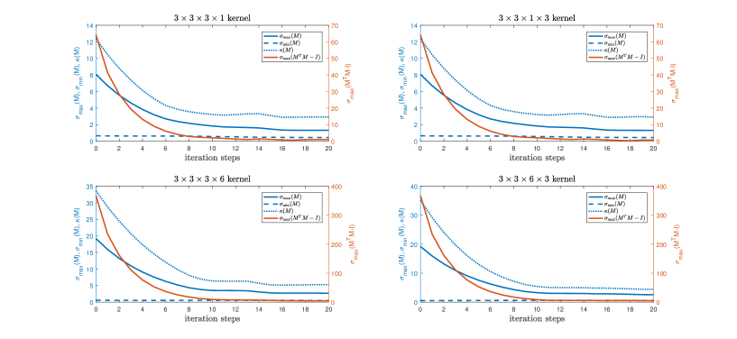
Figure 3.1: Example 1: Convergence of $\sigma_{max}(M),\sigma_{min}(M),\kappa(M),\sigma_{max}(M^{T}M-I)$ for four kernel sizes

Example 2: We consider kernels of size $3\times 3\times 3\times 1$ and use ${\cal R}_{\alpha}(K)=\sigma_{max}(M^{T}M-\alpha I)$ with $\alpha=0.1,1,5,$ and $10$. We present in Figure 3.2 the convergence of $\sigma_{max}(M^{T}M-I)$ (red solid line) on the right axis scale, and $\sigma_{max}(M)$ (blue solid line), $\sigma_{min}(M)$ (blue dashed line), and the condition number $\kappa(M)$ (blue dotted line) on the left axis scale.

For all values of $\alpha$, $\sigma_{max}(M^{T}M-\alpha I)$ converges to a value dependent on $\alpha$. The condition number $\kappa(M)$ and $\sigma_{max}(M^{T}M-\alpha I)$ decreases accordingly. For the larger values of $\alpha$, the convergence appears faster. For example, for $\alpha=5$ and $10$, $\sigma_{max}(M^{T}M-\alpha I)$ reaches minimum a little below the values of $\alpha$ at the $6$th and the $4$th iteration. Even though the minimum values are also larger than other cases, it has similar effect in reducing $\kappa(M)$ and $\sigma_{max}(M^{T}M-\alpha I)$ as suggested by Theorem 2.1. An interesting observation is that after $\sigma_{max}(M^{T}M-\alpha I)$ reaches a value smaller than $\alpha$, it increases back to a level of $\alpha$. It appears there may be a theoretical barrier to reducing $\sigma_{max}(M^{T}M-\alpha I)$ much below $\alpha$.

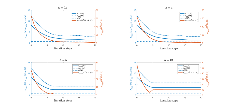
Figure 3.2: Example 2: Convergence of $\sigma_{max}(M),\sigma_{min}(M),\kappa(M),\sigma_{max}(M^{T}M-\alpha I)$ for different $\alpha$

4 Conclusions

In this paper, we have considered how to regularize the weights of convolutional layers in convolutional neural networks. The goal is to constrain the singular values of the structured transformation matrix corresponding to a convolutional kernel to be neither too large nor too small. We have devised the penalty function and proposed the gradient decent method for the convolutional kernel to achieve this. Numerical examples demonstrate its effectiveness for different size of convolution kernels. We have also proposed a more general penalty function ${\cal R}_{\alpha}(K)$ and have observed some interesting behavior with respect to the choice of $\alpha$. It will be interesting to further investigate this, which is left to a future work.

5 Acknowledgements

The authors are grateful to Professor Xinguo Liu at Ocean University of China and Professor Beatrice Meini at University of Pisa for their valuable suggestions.

References

- [1] M. Arjovsky, A. Shah, and Y. Bengio. Unitary evolution recurrent neural networks. In ICML, 2016.
- [2] J. Baglama and L. Reichel. Augmented implicitly restarted Lanczos bidiagonalization methods. SIAM J. Sci. Comp., 27:19–42, 2005.
- [3] Andrew Brock, Theodore Lim, James M Ritchie, and Nick Weston. Neural photo editing with introspective adversarial networks. In ICLR, 2017.
- [4] R. Chan and M. Ng, Conjugate Gradient Methods for Toeplitz Systems, SIAM Review, 38(3): 427-482, 1996.
- [5] R. Chan and X. Jin, An Introduction to Iterative Toeplitz Solvers, SIAM, Philadelphia, 2007.
- [6] Moustapha Cisse, Piotr Bojanowski, Edouard Grave, Yann Dauphin, Nicolas Usunier. Parseval Networks: Improving Robustness to Adversarial Examples. In ICML, 2017.
- [7] Vincent Dumoulin, Francesco Visin. A guide to convolution arithmetic for deep learning. ArXiv, 2018.
- [8] G.-H. Golub and C.-F. Van Loan, Matrix computations, Johns Hopkins University Press, Baltimore, 2012.
- [9] I. J. Goodfellow, J. Shlens, and C. Szegedy. Explaining and harnessing adversarial examples. In ICLR, 2015.
- [10] K. Helfrich, D. Willmott, and Q. Ye. Orthogonal Recurrent Neural Networks with Scaled Cayley Transform, In ICML, 2018.
- [11] S. Hochreiter, Y. Bengio, P. Frasconi, J. Schmidhuber, et al. Gradient flow in recurrent nets: the difficulty of learning long-term dependencies, In Field Guide to Dynamical Recurrent Networks, IEEE Press, 2001.
- [12] X. Jin, Developments and Applications of Block Toeplitz Iterative Solvers, Science Press, Beijing, 2002.
- [13] Kovaevi, Jelena and Chebira, Amina. An introduction to frames, Now Publishers Inc, Boston, 2008.
- [14] R. B. Lehoucq, D. C. Sorensen, and C. Yang, ARPACK Users’ Guides, Solution of Large Scale Eigenvalue Problems with Implicitly Restarted Arnoldi Method, SIAM, Philadelphia, 1998.
- [15] Q. Liang and Q. Ye, Computing singular values of large matrices with an inverse-free preconditioned krylov subspace method, Electronic Transactions on Numerical Analysis, 42: 197–221, 2014.
- [16] K.D. Maduranga, K. Helfrich and Q. Ye, Complex Unitary Recurrent Neural Networks using Scaled Cayley Transform, In AAAI, 2019.
- [17] Takeru Miyato, Toshiki Kataoka, Masanori Koyama, Yuichi Yoshida. Spectral Normalization for Generative Adversarial Networks. In ICLR, 2018.
- [18] Hanie Sedghi, Vineet Gupta and Philip M. Long. The Singular Values of Convolutional Layers. In ICLR, 2019.
- [19] G. W. Stewart. Matrix Algorithms: Volume II. Eigensystems, SIAM, 2001.
- [20] C. Szegedy, W. Zaremba, I. Sutskever, J. Bruna, D. Erhan, I. J. Goodfellow, and R. Fergus. Intriguing properties of neural networks. In ICLR, 2014.
- [21] Y. Tsuzuku, I. Sato, and M. Sugiyama. Lipschitz-Margin Training: Scalable Certification of Perturbation Invariance for Deep Neural Networks. In NIPS, 2018.
- [22] S. Wisdom, T. Powers, J. Hershey, J. Le Roux, and L. Atlas. Full-capacity unitary recurrent neural networks. In NIPS, 2016.
- [23] C. Zhang, S. Bengio, M. Hardt, B. Recht, and O. Vinyals. Understanding deep learning requires rethinking generalization. In ICLR, 2017.
- [24] Yuichi Yoshida, Takeru Miyato. Spectral Norm Regularization for Improving the Generalizability of Deep Learning, ArXiv 2017.