Testing macroscopic local realism using time-settings

Abstract

We show how one may test macroscopic local realism where, different from conventional Bell tests, all relevant measurements need only distinguish between two macroscopically distinct states of the system being measured. Here, measurements give macroscopically distinguishable outcomes for a system observable and do not resolve microscopic properties (of order $\hbar$). Macroscopic local realism assumes: (1) macroscopic realism (the system prior to measurement is in a state which will lead to just one of the macroscopically distinguishable outcomes) and (2) macroscopic locality (a measurement on a system at one location cannot affect the macroscopic outcome of the measurement on a system at another location, if the measurement events are spacelike separated). To obtain a quantifiable test, we define $M$-scopic local realism where the outcomes are separated by an amount $\sim M$. We first show for $N$ up to $20$ that $N$-scopic Bell violations are predicted for entangled superpositions of $N$ bosons (at each of two sites). Secondly, we show violation of $M$-scopic local realism for entangled superpositions of coherent states of amplitude $\alpha$, for arbitrarily large $M=\alpha$. In both cases, the systems evolve dynamically according to a local nonlinear interaction. The first uses nonlinear beam splitters realised through nonlinear Josephson interactions; the second is based on nonlinear Kerr interactions. To achieve the Bell violations, the traditional choice between two spin measurement settings is replaced by a choice between different times of evolution at each site.

Motivated by Schrodinger’s cat paradox s-cat , much effort has been devoted to testing quantum mechanics at a macroscopic level. Quantum superpositions of macroscopically distinguishable states, so-called cat-states, have been created in a number of different physical scenarios supmat . However, Leggett and Garg pointed out that a very strong test of macroscopic quantum mechanics would give a method to falsify all possible alternative theories satisfying the notion of macroscopic realism legggarg .

To address this problem, Leggett and Garg formulated inequalities Bell-2 , which if violated falsify a form of macroscopic realism now called macro-realism legggarg ; emary-review . Leggett and Garg’s macro-realism combines two classical premises: The first premise is macroscopic realism (MR): For a system which has two macroscopically distinguishable states available to it, as identifiable by a measurement which gives one of two macroscopically distinguishable outcomes, the system must at any time be in one or other of these states i.e. it must be in a state which will lead to just one of the distinct outcomes. Macroscopic realism implies the existence of a hidden variable to predetermine outcomes of measurements that are macroscopically distinct legggarg . In Schrodinger’s paradox, the assumption of macroscopic realism is that Schrodinger’s cat is always dead or alive, prior to any measurement.

The second Leggett-Garg premise is “macroscopic noninvasive measurability”: a measurement can in principle distinguish which of the macroscopically distinguishable states the system is in, with a negligible effect on the subsequent macroscopic dynamics of the system. There have been violations of Leggett-Garg inequalities reported, including experimentally for superconducting qubits and single atoms jordan_kickedqndlg2 ; lgexpphotonweak ; Mitchell-1 ; lauralg ; bognoon ; massiveosci-1-1 ; NSTmunro ; robens ; emary-review ; manushan-cat-lg . A complication with the Leggett-Garg tests is the justification of the second “noninvasive measurability” premise for any practical measurement jordan_kickedqndlg2 ; lgexpphotonweak ; lauralg ; manushan-cat-lg ; legggarg .

In this paper, we show how a form of macroscopic realism may be tested using Bell inequalities Bell-2 . This represents an advance because here the second Leggett-Garg premise is replaced by the premise of macroscopic locality (ML), which leads to a stronger test of macroscopic realism: Where a measurement at one location gives one of two macroscopically distinguishable outcomes, and macroscopic realism is assumed, then macroscopic locality implies that a measurement made at another location cannot change the predetermined (hidden-variable) value for the measurement at the first location. This is provided the two measurement events are spacelike separated. In Schrodinger’s paradox, macroscopic locality implies a measurement on a second separated system could not (instantly) change the cat from dead to alive, or vice versa. The combined premises of MR and ML constitute the premise of macroscopic local realism (MLR) MLR ; mlr-uncertainty ; mdrmlr2 .

Specifically, we explain how the predictions of quantum mechanics are incompatible with those of macroscopic local realism for systems prepared in certain macroscopic entangled superposition states. To obtain a quantifiable test for cases where macroscopically distinct outcomes are not realistic, we define $M$-scopic local realism to apply where the outcomes are separated by an amount of order $M$. The important feature of the Bell tests presented in this paper is that the outcomes of all relevant measurements involved in the Bell inequality correspond to macroscopically distinct states of the system being measured i.e. measurements only need to distinguish between the two extreme states of a macroscopic superposition state (a “cat state”). The measurements do not resolve at the level of $\hbar$. We consider two cases. In the first, measurements detect either all of $N$ bosons in one mode, or all $N$ bosons in a second mode. In the second case, the measurements distinguish between the coherent states (of amplitude $\alpha$) well separated in phase space (by, of order, $\alpha$). We determine violation of $N$-scopic local realism for $N$ up to $20$, and of $\alpha$-scopic local realism for $\alpha\rightarrow\infty$. The violations are possible, because we allow nonlinear dynamics at each of the separated sites, and consider different local time (or nonlinearity) settings.

The Bell tests of this paper differ from previous Bell tests for macroscopic systems meso-bell-higher-spin-cat-states-bell , including those for superpositions of macroscopically distinct states cat-bell-wang ; cat-bell , which almost invariably require at least one measurement that resolves microscopic outcomes, or else involve a continuous range of outcomes mlr-uncertainty ; MLR ; cv-bell ; mdrmlr2 . These former tests are not in the spirit of Leggett and Garg, who considered only measurements distinguishing the two macroscopically distinct states that form an extreme macroscopic superposition state (so that the separation of outcomes well exceeds the level associated with the standard quantum limit ($\hbar$)). The results of this paper show that Bell violations can be predicted in this macroscopic regime. To the best of our knowledge, such tests have not been performed for $N>1$.

Bell inequality for macroscopic local realism: For spatially separated sites $A$ and $B$, we consider the two-qubit Bell state

$$|\psi_{\pm,+}\rangle_{AB} = (|1\rangle_{A}|\pm 1\rangle_{B}+|-1\rangle_{A}|\mp 1\rangle_{B})/\sqrt{2}$$

$$|\psi_{\pm,-}\rangle_{AB} = (|1\rangle_{A}|\pm 1\rangle_{B}-|-1\rangle_{A}|\mp 1\rangle_{B})/\sqrt{2}$$ (1)

where $|1\rangle_{A}=|N\rangle_{a}|0\rangle_{a_{2}}$, $|1\rangle_{B}=|N\rangle_{b}|0\rangle_{b_{2}}$, $|-1\rangle_{A}=|0\rangle_{a}|N\rangle_{a_{2}}$, $|-1\rangle_{B}=|0\rangle_{b}|N\rangle_{b_{2}}$. Here, we consider two modes denoted $a$ and $a_{2}$, and $b$ and $b_{2}$, at each location $A$ and $B$ respectively. $|n\rangle_{a/b}$ is the number state for the mode denoted $a/b$. We next define the action of a hypothetical nonlinear beam splitter (NBS) at site $A$. For an initial state $|N\rangle_{a}|0\rangle_{a_{2}}$, the state after the hypothetical NBS interaction is

$$|\psi(t_{a})\rangle = \hat{U}_{A}|N\rangle_{a}|0\rangle_{a_{2}}$$

$$= e^{i\varphi(t_{a})}(\cos t_{a}|N\rangle_{a}|0\rangle_{a_{2}}-i\sin t_{a}|0\rangle_{a}|N\rangle_{a_{2}})$$

where we have introduced a unitary operator $\hat{U}_{A}$ and $t_{a}$ is the time of interaction in scaled units. A similar NBS interaction is assumed to take place at site $B$.

$$|\psi(t_{b})\rangle = \hat{U}_{B}|N\rangle_{b}|0\rangle_{b_{2}}$$

$$= e^{i\varphi(t_{b})}(\cos t_{b}|N\rangle_{b}|0\rangle_{b2}-i\sin t_{b}|0\rangle_{b}|N\rangle_{b2})$$

Assuming the incoming state to be $|\psi_{+,\pm}\rangle_{AB}$, the final state is

$$\hat{U}_{A}\hat{U}_{B}|\psi_{AB}\rangle=e^{i\varphi}(\cos t_{\pm}|\psi_{+,\pm}\rangle-i\sin t_{\pm}|\psi_{-,\pm}\rangle)$$ (4)

where $t_{\pm}=t_{a}\pm t_{b}$ and $\varphi$ is a phase factor. Defining the “spin” at $A$ ($B$) as $\pm 1$ if the system is detected as $|\pm 1\rangle_{A}$ ($|\pm 1\rangle_{B})$, the expectation value for the spin product is $E(t_{a},t_{b})=\cos 2(t_{\pm})$. Where $N$ is large, the assumption of macroscopic local realism (MLR) will imply the Clauser-Horne-Shimony-Holt (CHSH) Bell inequality $B\leq 2$ CShim-review , where

$$B=E(t_{a},t_{b})-E(t_{a},t^{\prime}_{b})+E(t^{\prime}_{a},t_{b}^{\prime})+E(t^{\prime}_{a},t_{b})$$ (5)

Here we note there are two choices of interaction times at each location: $t_{a}$, $t^{\prime}_{a}$ at $A$, and $t_{b}$, $t_{b}^{\prime}$ at $B$. This inequality is derived assuming that before the measurement at the selected time $t$, the system is in one or other states described by $|\pm 1\rangle$ at each site (MR), and that there is no nonlocal effect changing the state due to the measurement at the other location (ML). For $N$ large, the qubits $|\pm 1\rangle_{A/B}$ correspond to macroscopically distinct outcomes for all choices of $t_{a}$ and $t_{b}$, and the violation of the Bell inequality will falsify MLR. The solution for $E(t_{a},t_{b})$ will violate the inequality for suitable choices of $t_{a}$ and $t_{b}$ CShim-review .

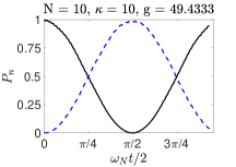
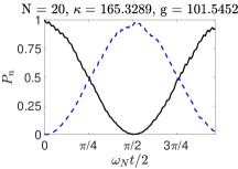
Figure 1: Solutions for the Hamiltonian $H_{NL}^{(A)}$ after a time $t$ with initial state $|N\rangle_{a}|0\rangle_{a_{2}}$. $P_{N}$ (black solid line) is the probability for all $N$ bosons to be in mode $a$; $P_{0}$ (blue dashed line) is the probability for all $N$ bosons to be in mode $a_{2}$. The parameters identify regimes optimal, or near-optimal, for the nonlinear beam splitter interaction eq. (Testing macroscopic local realism using time-settings), where $P_{N}+P_{0}\sim 1$ and $P_{N}\sim\cos^{2}\omega_{N}t$. Solutions for $N=1$ (all $\kappa,$$g$); $N=2$, $\kappa=1$, $g=30$; $N=5$, $\kappa=20$, $g=333.333$; and $N=7$, $\kappa=18.23$, $g=47.85$ are similar to the left plot.

Nonlinear beam splitter (NBS) for $N$ bosons: The above is a straighforward extension of Bell’s work, except for the nontrivial complication that it needs to be shown that the hypothetical NBS interaction can be predicted in quantum mechanics, to a sufficient degree that allows the violation of the Bell inequality. To do this, we consider at $A$ two incoming fields ($a$ and $a_{2}$), which interact according to the nonlinear Josephson Hamiltonian josHam-lmg ; josHam-collett-steel

$$H_{NL}^{(A)}=\kappa(\hat{a}^{\dagger}\hat{a}_{2}+\hat{a}\hat{a}_{2}^{\dagger})+g\hat{a}^{\dagger 2}\hat{a}^{2}+g\hat{a}_{2}^{\dagger 2}\hat{a}_{2}^{2}$$ (6)

Here, $\hat{a}$, $\hat{a}_{2}$ are the boson operators for the corresponding fields $a$, $a_{2}$, modelled as single modes. A similar interaction $H_{NL}^{(B)}$ is assumed for the fields $b$ and $b_{2}$ at $B$. Such an interaction can be achieved with Bose-Einstein condensates (BEC) or superconducting circuits oberoscexp ; pol. ; superconducting-nonlinear ; superfluid ; two-well-cm ; carr-two-well ; josHam-collett-steel ; josHam-lmg ; bognoon ; lauralg . For certain choices of $g$ and $\kappa$, we find that the interaction (6) acts as a nonlinear beam splitter, where the input $|N\rangle_{a}|0\rangle_{a_{2}}$ after a time $t$ gives, to a good approximation, the output of eqn (Testing macroscopic local realism using time-settings) (Figure 1). We introduce a scaled time $t_{a}=\omega_{N}t$ where $\omega_{N}=2g\frac{N}{\hbar(N-1)!}\left(\frac{\kappa}{g}\right)^{N}$ carr-two-well .

$N$-scopic Bell tests for $N$ bosons: It now remains to determine whether the realisation of the NBS (which is never exact) can actually allow a violation of the Bell inequality. We first examine a specific method of preparation of (1) noon-cond-pryde-white ; reid-walls ; Ou-mandel ; laura-paper ; int-nonlocality-bS . We consider that the two separated modes $a$ and $b$ are prepared at time $t=0$ in the NOON state $|\psi\rangle_{ab}=\frac{1}{\sqrt{2}}(|N\rangle_{a}|0\rangle_{b}+e^{i\vartheta}|0\rangle_{a}|N\rangle_{b})$ opticalNOON-1 ; heralded-noon ; laura-paper ; herald-noon and that the modes $a_{2}$ and $b_{2}$ are prepared similarly, in the NOON state $\frac{1}{\sqrt{2}}(|0\rangle_{a_{2}}|N\rangle_{b_{2}}+e^{-i\pi/2}|N\rangle_{a_{2}}|0\rangle_{b_{2}})$ (Figure 2). Assuming optimal NBS parameters, the final state is $|\psi_{f-}\rangle=\hat{U}_{A}\hat{U}_{B}|\psi\rangle_{ab}|\psi\rangle_{a_{2}b_{2}}$. For an alternative method using the NBS interaction, refer to the Supplemental Materials supmat . We find ($\phi_{-}$ is a phase factor)

$$|\psi_{f-}\rangle = \frac{e^{i\phi_{-}}}{\sqrt{2}}\Bigl{(}\cos t_{-}(|\psi_{-,-}\rangle{\color[rgb]{0,0,0}{\color[rgb]{0,0,0}-}}i\sin t_{-}|\psi_{+,-}\rangle\Bigl{)}$$ (7)

$$+\frac{1}{\sqrt{2}}|\varphi_{-}\rangle_{2N}$$

$|\varphi_{-}\rangle_{2N}$ are states with all $2N$ bosons at site $A$, or all $2N$ bosons at site $B$.

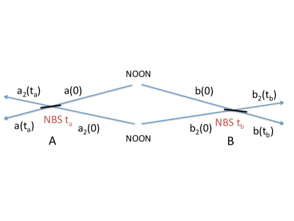
Figure 2: The macroscopic entangled state (1) can be generated conditionally by interfering two NOON states. The $t_{a}$ and $t_{b}$ are time settings selected for the nonlinear beam splitter (NBS) at each site, $A$ and $B$.

To test $N$-scopic local realism, the mode numbers at the final outputs $a(t_{a})$, $a_{2}(t_{a})$, $b(t_{b})$ and $b_{2}(t_{b})$ are measured (Figure 2), for a given setting of the times $t_{a}$ and $t_{b}$ at each site. The measurement events at $A$ and $B$ are spacelike separated if the distance between them is sufficiently great, taking into account the times $t_{a}$ and $t_{b}$ required for the NBS interactions. At $A$, we denote by $+$ the outcome of detecting $N$ bosons at location $a$, and $0$ bosons at $a_{2}$. A similar outcome $+$ is defined for $B$. (The state $|\varphi_{-}\rangle_{2N}$ thus becomes irrelevant). We define the joint probability $P_{++}$ for the outcome $+1$ at both sites $A$ and $B$. We also specify $P_{+}^{A}$ as the marginal probability for the outcome $+$ at $A$, and $P_{+}^{B}$ as the marginal probability for the outcome $+$ at $B$. At each site $A$ and $B$, observers independently select a time of evolution $t_{a}$ and $t_{b}$ for the NBS interaction.

It is evident from the expression (7) that the outcomes of a measurement of mode number at each detector are always one of $0$, $N$ or $2N$ (Figure 3), which are macroscopically distinguishable as $N\rightarrow\infty$. The assumption of $N$-scopic LR (which becomes MLR as $N\rightarrow\infty$) thus implies the validity of a local hidden variable theory, where the system at each site is predetermined to be in one of the states with mode number $0$, $N$, or $2N$. The Clauser-Horne (CH) Bell inequality $S\leq 1$ CShim-review is predicted to hold for such a local hidden variable theory, where laura-paper

$$S = \frac{P_{++}(t_{a},t_{b})-P_{++}(t_{a},t^{\prime}_{b})+P_{++}(t_{a}^{\prime},t{}_{b})+P_{++}(t^{\prime}_{a},t^{\prime}_{b})}{P_{+}^{A}(t_{a}^{\prime})+P_{+}^{B}(t_{b})}$$

Assuming ideal nonlinear beam splitters, the state $|\psi_{f-}\rangle$ gives $P_{++}=\frac{1}{4}\sin^{2}(t_{a}-t_{b})$ and $P_{+}^{A}=P_{+}^{B}=\frac{1}{4}$. For $t_{a}=0$, $t_{a}^{\prime}=2\varphi$, $t_{b}=\varphi$ and $t_{b}^{\prime}=3\varphi$, the quantum state $|\psi_{f-}\rangle$ of (7) predicts $S=\frac{3\sin^{2}(\varphi)-\sin^{2}(3\varphi)}{2}$. $S$ maximizes at $S=1.207$ for $\varphi=\pi/16$, giving a violation of the CH Bell inequality.

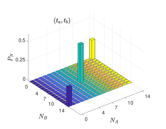
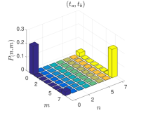
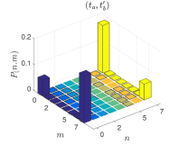
Figure 3: Top: Probability distribution $P_{N}$ for the joint detection of $N_{A}$ and $N_{B}$ bosons at the sites $A$ and $B$ (refer Fig. 2). Here $t_{a}$, $t_{b}$, $t_{a}^{\prime}$, $t_{b}^{\prime}$ and $\varphi$ are specified in the text. $N=7$, $\kappa=18.23$, $g=47.85$. The distribution is unchanged for settings $(t^{\prime}_{a},t_{b})$, $(t^{\prime}_{a},t^{\prime}_{b})$ and $(t_{a},t^{\prime}_{b})$. Lower: The joint probability $P(n,m)$ of detecting $n$ bosons in mode $a$ and $m$ bosons in mode $b$, and $N$ bosons in total at site $A$. The figures for settings $(t^{\prime}_{a},t_{b})$, $(t^{\prime}_{a},t^{\prime}_{b})$ are identical to those of $(t_{a},t_{b})$. Similar plots are obtained for all parameters given in Fig. 1.

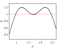
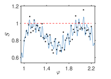
Figure 4: Violation of the CH-Bell inequality (LABEL:eq:ch-bell-ineq) is obtained when $S>1$. Left graph is for $N=10$, $g=49.433$, $\kappa=10$. Plots for $N=1$ (all $\kappa$ and $g$); $N=2$, $\kappa=1$, $g=30$; $N=5$, $\kappa=20$, $g=333.333$; and $N=7$, $\kappa=18.23$, $g=47.85$ which give ideal two-state oscillatory behaviour (Fig. 1) are almost indistinguishable. Where the values are not quite optimal, rapid oscillations of small amplitude appear. This is shown in the right graph for $N=20$, $\kappa=165$ and $g=101$.

In practice, the ideal regime giving the precise solution (Testing macroscopic local realism using time-settings) for the nonlinear beam splitters is unattainable, for $N>1$, since probabilities for other than $0$ or $N$ bosons in each mode are not precisely zero. In Figures 3 and 4, we present actual predictions for $S$, using the Hamiltonian $H_{NL}$. For large $gN/\kappa$, where care is taken to optimize for the NBS regime given by (Testing macroscopic local realism using time-settings), the Bell violations are predicted, as shown in Figure 4. To test N-scopic LR, one requires to establish that the outcomes of mode number are distinct by $N$, for each of the joint probabilities $P(t_{a},t_{b})$ comprising $S$. Figure 3 highlights this feature in the optimal parameter space. The probabilities for results other than $0$ and $N$ (and $2N$, for Figure 3a) are negligible (and can rigorously be shown to have no effect on the violation, using the methods of eric_marg ; legggarg ).

Macroscopic Bell tests using cat-states: To examine macroscopic behaviour, we consider the Bell cat-state

$$|\psi\rangle=N(|+\rangle_{a}|+\rangle_{b}-|-\rangle_{a}|-\rangle_{b})$$ (9)

where $|+\rangle_{a}=-e^{i\pi/6}(|e^{i\pi/3}\alpha\rangle_{a}+|e^{-i\pi/3}\alpha\rangle_{a})/\sqrt{2}$, $|-\rangle_{b}=ie^{-i\pi/6}(|-e^{i\pi/3}\beta\rangle_{b}+|-e^{-i\pi/3}\beta\rangle_{b})/\sqrt{2}$, $|-\rangle_{a}=|-\alpha\rangle$, $|+\rangle_{b}=-i|\beta\rangle$ and $|\alpha\rangle$, $|\beta\rangle$ are coherent states for two modes labelled $a$ and $b$. $N$ is a normalisation constant. Since we consider $\alpha,\beta$ to be real and $\alpha$, $\beta\rightarrow\infty$, $|\pm\rangle_{a}$ become orthogonal, and similarly $|\pm\rangle_{b}$. This then corresponds to the state $|\psi_{+,-}\rangle_{AB}$ of (1), where $|\pm\rangle_{A/B}=|\psi_{\pm}\rangle_{a/b}$.

To realise a nonlinear interaction (NBS), we propose at each site the nonlinear Kerr interaction $H_{NL}^{(A/B)}=\Omega\hat{n}_{A/B}^{2}$ where $\hat{n}_{A}=\hat{a}^{\dagger}\hat{a}$ and $\hat{n}_{B}=\hat{b}^{\dagger}\hat{b}$ yurke-stoler ; wrigth-walls-gar ; kirchmair ; collapse-revival-bec . For systems prepared in coherent states $|\alpha\rangle$ the interaction after certain times leads to the formation of cat-states where (for large $\alpha$) the system is in a superposition of macroscopically distinct coherent states in phase space. At any time, one can perform quadrature phase amplitude measurements $\hat{X}_{A}={\color[rgb]{1,0,0}{\color[rgb]{0,0,1}{\color[rgb]{0,0,0}\frac{1}{\sqrt{2}}}}}(\hat{a}+\hat{a}^{\dagger})$ and $\hat{X}_{B}={\color[rgb]{1,0,0}{\color[rgb]{0,0,1}{\color[rgb]{0,0,0}\frac{1}{\sqrt{2}}}}}(\hat{b}+\hat{b}^{\dagger})$ at each site. The “spin” result $\hat{s}$ is taken to be $+1$ if the result for such a measurement is $>0$, and $-1$ otherwise. A state with outcome $\pm 1$ is denoted $|\pm\rangle$. At time $t^{\prime}_{A}=\pi/(3\Omega)$, if the initial state is $|\alpha\rangle$, the state at $A$ is manushan-cat-lg

$$|\psi(t^{\prime}_{A})\rangle = -i{\color[rgb]{0,0,1}{\normalcolor\sqrt{\frac{1}{3}}|-\rangle_{a}+\sqrt{\frac{2}{3}}|+\rangle_{a}}}$$ (10)

For an initial state $|\beta\rangle$, the state at time $t^{\prime}_{b}=2\pi/(3\Omega)$ is

$${\normalcolor|\psi(t^{\prime}_{B})\rangle} {\normalcolor=} \sqrt{\frac{1}{3}}|+\rangle_{b}-i\sqrt{\frac{2}{3}}|-\rangle_{b}$$ (11)

We select $t_{A}=0$ and $t^{\prime}_{A}=\pi/(3\Omega)$, and $t_{B}=0$ and $t^{\prime}_{B}=2\pi/(3\Omega)$. The final state after the Kerr dynamics gives (as $\alpha=\beta\rightarrow\infty$): $E(t_{A},t{}_{B})=1$; $E(t_{A},t^{\prime}{}_{B})=-1/3$; $E(t^{\prime}_{A},t{}_{B})=1/3$; $E(t^{\prime}_{A},t^{\prime}{}_{B})=7/9$. This implies violation of the Bell inequality (5) with $B=2.44$ supmat .

Figure 5 gives the complete predictions for arbitrary $\alpha$, $\beta$, accounting for the full effect of nonorthogonality of the coherent states. The outcomes of measurements of $\hat{s}$ (the sign of $\hat{X}$) are macroscopically distinct, corresponding to macroscopically distinguishable states in phase space, for all of the choices of time-settings, as $\alpha,$$\beta$ becomes large (Figure 5a and supmat ). Violations of $\alpha$-scopic local realism are predicted for all $\alpha=\beta>2$ (Figure 5b) supmat .

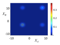
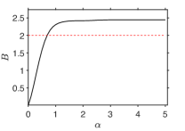
Figure 5: Left: A contour plot for the joint probability distribution of the quadrature phase amplitudes $X_{A}$ and $X_{B}$ at times $t_{a}=\pi/3\Omega$ and $t_{b}=0$. The four outcomes depicted are macroscopically distinct for $\alpha$ large. Here $\alpha=\beta=5$. The distributions for the remaining 3 pairs of times are similar supmat . Right: The corresponding violation $B>2$ of the Bell inequality eq. (5) for arbitrarily large $\alpha=\beta$.

Conclusion: We have argued that violation of the Bell inequality falsifies MLR, because the outcomes measured at location $A$ ($B$) are macroscopically distinct: A critic might claim differently. They may argue that a microscopic nonlocal quantum effect is translated by the dynamics (which occurs over a time $t_{a/b}$) into a macroscopic effect, which is then registered by the detectors. This criticism could be further explored supmat .

Preparing entangled macroscopic superposition states where $A$ and $B$ are spatially separated is a challenge. This is addressed if the initial NOON state of Figure 2 has separated modes (for $N=2$, the Hong-Ou-Mandel effect might be useful heralded-noon ).For a Rb BEC, the timescales required for the nonlinear beam splitter become inaccessibly long oberoscexp ; carr-two-well . The nonlinear beam splitter is however likely achievable using superconducting circuits to obtain high nonlinearities bellcatexp ; superconducting-nonlinear . In fact, a two-mode cat-state similar to (9) has been generated cat-bell-wang (although without spatial separation) and the dynamics of (10) and (11) realized for BECs and microwave fields collapse-revival-bec ; kirchmair . Noting that macroscopic realism (MR) is suggestive of the validity macroscopic locality (ML) det-bell , an experimental test, even if without spatial separation, for moderate $N$ or $\alpha$, would be of interest.

- (1) E. Schroedinger, 23, 807 (1935). F. Frowis et al., Rev. Mod. Phys. 90, 025004 (2018).
- (2) M. Brune et al., Phys. Rev. Lett. 77, 4887 (1996). C. Monroe et al., Science 272, 1131 (1996). A. Ourjoumtsev et al., Nature 448, 784 (2007). D. Leibfried et al., Nature 438, 04251 (2005). T. Monz et al., Phys. Rev. Lett. 106, 130506 (2011). J. Lavioe et al., New J. Phys 11, 073051 (2009). H. Lu et al., Phys. Rev. A 84, 012111 (2011). A. Omran et al., arXiv:1905.0572v2 (2019).
- (3) J. Friedman et al., Nature 406 43 (2000). A. Palacios-Laloy, et al.,Nature Phys. 6, 442 (2010).
- (4) P. Walther et al., Nature 429, 158 (2004). M. W. Mitchell, J. S. Lundeen, and A. M. Steinberg, Nature 429, 161 (2004). J. P. Dowling, Contemporary Physics 49, 125 (2008).
- (5) S. Slussarenko et al., Nature Photonics 11, 700 (2017).
- (6) M. Stobinska et al., Phys. Rev. A 86 063823 (2012). T. Sh. Iskhakov et al., New J. Phys. 15, 093036 (2013).
- (7) B. Vlastakis et al., Science 342, 607 (2013).
- (8) C. Wang et al., Science 352, 1087 (2016).
- (9) A. Leggett and A. Garg, Phys. Rev. Lett. 54, 857 (1985).
- (10) A. N. Jordan, A. N. Korotkov, and M. Buttiker, Phys. Rev. Lett. 97, 026805 (2006). N. S. Williams and A. N. Jordan, Phys. Rev. Lett. 100, 026804 (2008).
- (11) C. Emary, N. Lambert, and F. Nori, Rep. Prog. Phys 77, 016001 (2014). Z. Q. Zhou, S. Huelga, C-F Li, and G-C Guo, Phys. Rev. Lett. 115, 113002 (2015).G. Waldherr et al., Phys.Rev. Lett. 107, 090401 (2011).
- (12) J. Dressel et al., Phys. Rev. Lett. 106, 040402 (2011). M. E. Goggin, et al., Proc. Natl. Acad. Sci. 108, 1256 (2011).
- (13) G. C. Knee et al., Nat. Commun. 7, 13253 (2016).
- (14) C. Robens, W. Alt, D. Meschede, C. Emary, and A. Alberti, Phys. Rev. X 5, 011003 (2015).
- (15) A. Asadian, C. Brukner, and P. Rabl, Phys. Rev. Lett. 112, 190402 (2014).
- (16) C. Budroni et al., Phys. Rev. Lett. 115, 200403 (2015).
- (17) B. Opanchuk et al., Phys. Rev. A 94, 062125 (2016).
- (18) L. Rosales-Zárate et al., Phys. Rev. A 97, 042114 (2018).
- (19) M. Thenabadu and M. D. Reid, Phys. Rev. A 99, 032125 (2019).
- (20) J. S. Bell, Physics 1, 195 (1964). N. Brunner et al., Rev. Mod. Phys. 86, 419 (2014).
- (21) See discussions on determinism in H. M. Wiseman, Journ. Phys A 47, 424001 (2014).
- (22) M. D. Reid, Phys. Rev. Lett. 84, 2765 (2000); Phys. Rev. A 62, 022110 (2000).
- (23) M. Reid, Z. Naturforsch. A 56, 220 (2001).
- (24) M. D. Reid, Phys. Rev. A 97, 042113 (2018).
- (25) N. D. Mermin, Phys. Rev. D 22, 356 (1980). J. C. Howell, A. Lamas-Linares, and D. Bouwmeester, Phys. Rev. Lett. 88, 030401 (2002). P. D. Drummond, Phys. Rev. Lett. 50, 1407 (1983). M. D. Reid and W. J. Munro, Phys. Rev. Lett. 69, 997 (1992). M. D. Reid, W. J. Munro, and F. De Martini, Phys. Rev. A 66, 033801 (2002).
- (26) N. D. Mermin, Phys. Rev. Lett. 65, 1838 (1990). A. Gilchrist et al. , Phys. Rev. A60, 4259 (1999). K. Wodkiewicz, New Journal of Physics 2, 21 (2000). G. Svetlichny, Phys. Rev. D35, 3066 (1987). D. Collins et al., Phys. Rev. Lett. 88, 170405 (2002). C. Wildfeuer, A. Lund and J. Dowling, Phys. Rev. A 76, 052101 (2007). F. Toppel, M. V. Chekhova, and G. Leuchs, arXiv:1607.01296 [quant-ph] (2016).
- (27) U. Leonhardt and J. Vaccaro, J. Mod. Opt. 42, 939 (1995). A. Gilchrist, P. Deuar and M. Reid, Phys. Rev. Lett. 80 3169 (1998). K. Banaszek and K. Wodkiewicz, Phys. Rev. Lett. 82 2009 (1999). Oliver Thearle et al., Phys. Rev. Lett. 120, 040406 (2018). A. Ketterer, A. Keller, T. Coudreau, and P. Milman, Phys. Rev. A 91, 012106 (2015). A.S. Arora and A. Asadian, Phys. Rev. A 92, 062107 (2015).
- (28) J. F. Clauser and A. Shimony, Rep. Prog. Phys. 41, 1881 (1978). J. F. Clauser and M. A. Horne, Phys. Rev. D10, 526, (1974).
- (29) H. J. Lipkin, N. Meshkov, and A. J. Glick, Nucl. Phys. 62 188 (1965).
- (30) M. Steel and M. J. Collett, Phys. Rev. A 57, 2920 (1998).
- (31) L. D. Carr, D. R. Dounas-Frazer, and M. A. Garcia-March, Europhys. Lett. 90, 10005 (2010).
- (32) M. Albiez et al., Phys. Rev. Lett. 95 010402 (2005).
- (33) K. K. Likharev, Rev. Mod. Phys. 51, 101 (1979). S. Zeytinoglu et al., Phys. Rev. A 91, 043846 (2015). C. Eichler et al., Phys. Rev. Lett., 113, 11502 (2014).
- (34) S. Backhaus et al., Nature 392, 687 (1998).
- (35) M. Abbarchi et al., Nature Physics 9, 275 (2013).
- (36) J. I. Cirac et al., Phys. Rev. A 57, 1208 (1998). G. J. Milburn et al., Phys. Rev. A 55, 4318 (1997). J. Dunningham and K. Burnett, Journ. Modern Optics, 48, 1837, (2001). D. Gordon and C. M. Savage, Phys. Rev. A 59, 4623, (1999). T. J. Haigh, A.J. Ferris, and M. K. Olsen, Opt. Commun. 283, 3540 (2010).
- (37) Z. Y. Ou and L. Mandel, Phys. Rev. Lett. 61, 50 (1988).
- (38) M. D. Reid and D. F. Walls, Phys. Rev. A 34, 1260 (1986). Y. H. Shih and C. O. Alley, Phys. Rev. Lett. 61, 2921 (1988).
- (39) G. J. Pryde and A. G. White, Phys. Rev. A 68, 052315 (2003). A. E. B. Nielsen and K. Mølmer, Phys. Rev. A 75, 063803 (2007).
- (40) M. Horne, A. Shimony, and A. Zeilinger, Phys. Rev. Lett. 62, 2209 (1989). S. M. Tan and D. F. Walls, Phys. Rev. Lett. 66, 252 (1991).
- (41) L. Rosales-Zarate et al. Phys. Rev. A90, 022109 (2014).
- (42) C. K. Hong, Z. Y. Ou and L. Mandel, Phys. Rev. Lett. 59, 2044 (1987). R. Lopes et al., Nature 520, 66 (2015). R. J. Lewis-Swan and K. V. Kheruntsyan, Nat. Commun. 5, 3752 (2014).
- (43) Refer to Supplemental Materials.
- (44) E. G. Cavalcanti and M. D. Reid, Phys. Rev. Lett., 97, 170405 (2006); Phys. Rev. A. 77, 062108 (2008). C. Marquardt et al., Phys. Rev. A 76 030101 (2007).
- (45) B. Yurke and D. Stoler, Phys. Rev. Lett. 57, 13 (1986).
- (46) E. Wright, D. Walls and J. Garrison, Phys. Rev. Lett. 77, 2158 (1996).
- (47) M. Greiner et al., Nature 419, 51 (2002).
- (48) G. Kirchmair et al., Nature 495, 205 (2013).