Relativistic wind accretion onto a Schwarzschild black hole

Abstract

We present a novel analytic model of relativistic wind accretion onto a Schwarzschild black hole. This model constitutes a general relativistic extension of the classical model of wind accretion by Bondi, Hoyle and Lyttleton (BHL). As in BHL, this model is based on the assumptions of steady state, axisymmetry and ballistic motion. Analytic expressions are provided for the wind streamlines while simple numerical schemes are presented for calculating the corresponding accretion rate and density field. The resulting accretion rate is greater in the relativistic model when compared to the Newtonian BHL one. Indeed, it is two times greater for asymptotic wind speeds $v_{\infty}\geq 0.4\,\mathrm{c}$ and more than an order of magnitude greater for $v_{\infty}\geq 0.8\,\mathrm{c}$. We have compared this full relativistic model versus numerical simulations performed with the free GPL hydrodynamics code aztekas (aztekas.org ©2008 Sergio Mendoza & Daniel Olvera and ©2018 Alejandro Aguayo-Ortiz & Sergio Mendoza) and found a good agreement for the streamlines in the upstream region of the flow and also, to within 10%, for the corresponding accretion rates.

1 Introduction

Accretion physics has become a basic tenet of astrophysics ever since it was recognized that the process of accretion, especially when compact objects are involved, is one of the most efficient mechanisms for converting rest mass energy into luminosity at work in our universe (Frank et al., 2002). Indeed, it has been established that a thin accretion disc around a non-rotating black hole can reprocess as much as 10 per cent of the accreted gas rest mass into electromagnetic radiation, while for a maximally rotating black hole this figure can reach up to 46 per cent (see e.g. Longair, 2011).

The simplest accretion scenario consists of the stationary, spherically-symmetric solution first discussed by Bondi (1952), where he considered an infinitely large homogeneous gas cloud steadily accreting onto a central gravitational object. The general relativistic extension of this model was developed by Michel (1972) who took a Schwarzschild black hole as the central accretor.

In the so-called wind accretion scenario, the spherical symmetry approximation is relaxed by considering a non-zero relative velocity between the central object and the accreted medium (cf. Edgar, 2004; Romero & Vila, 2014). As it turns out, even after assuming a steady state and axial symmetry, the problem becomes sufficiently complex as not to admit a full analytic solution in general. In the pioneering work of Hoyle & Lyttleton (1939) and Bondi & Hoyle (1944) (BHL hereafter), the authors provided an analytic model for supersonic wind accretion by adopting the so-called ballistic approximation, i.e. by neglecting pressure gradients and assuming that the fluid’s dynamics is solely dictated by the central object’s gravitational field. This approximation is well suited to describe highly supersonic flows given that, within this regime, incoming fluid elements cannot oppose pressure gradients readily, effectively following nearly free-fall trajectories.

Further analytic solutions to wind accretion problems have been found for a perfect fluid with a stiff equation of state in general relativity (Petrich et al., 1988) and for the corresponding non-relativistic case of an incompressible fluid (Tejeda, 2018).

The problem of wind accretion has also been the focus of various numerical studies, from both a Newtonian perspective (Hunt, 1971; Shima et al., 1985; Ruffert & Arnett, 1994; El Mellah & Casse, 2015; El Mellah et al., 2018) and in general relativity (Petrich et al., 1989; Font & Ibáñez, 1998; Zanotti et al., 2011; Lora-Clavijo & Guzmán, 2013; Gracia-Linares & Guzmán, 2015; Cruz-Osorio & Lora-Clavijo, 2016; Cruz-Osorio et al., 2017).

In this article we introduce a simple, analytic model for a supersonic wind accreting onto a non-rotating black hole (Schwarzschild spacetime). This model is a general relativistic extension of the BHL model and follows closely the methodology outlined in Mendoza et al. (2009), Tejeda et al. (2012, 2013). In that series of works, we presented an analytic model of the accretion flow of a rotating dust cloud infalling towards a central object, first in a Newtonian regime (Mendoza et al., 2009) and then in general relativity for a Schwarzschild black hole (Tejeda et al., 2012) and for a Kerr black hole (Tejeda et al., 2013). See Schroven et al. (2017) for a recent extension of this model considering the case of charged dust particles accreting onto a Kerr-Newman black hole.

The article is organised as follows. In Section 2 we give a brief review of the BHL model. In Section 3 we introduce the new relativistic wind model, and in Section 4 we present the comparison against relativistic hydrodynamic numerical simulations performed with the free GPL hydrodynamics code aztekas (Olvera & Mendoza, 2008; Aguayo-Ortiz et al., 2018). Finally, in Section 5 we summarize the work and present our conclusions. The Appendix A presents the results of the benchmark test of aztekas against Michel’s analytic model, as well as self-convergence and various resolution tests relevant to the present study.

2 Bondi-Hoyle-Lyttleton model

In this Section we give a brief overview of the BHL accretion model as its general relativistic extension constitutes the scope of the present work. The BHL model deals with a steady, supersonic wind accreting onto a gravitational object of mass $M$. Considering that the accretor is held fixed at the centre of coordinates, infinitely far away from the central object, the wind is homogeneous and characterized by a uniform density $\rho_{\infty}$ and wind speed $v_{\infty}$.

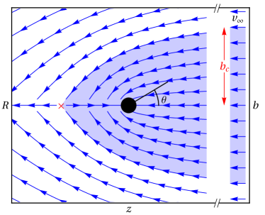
Figure 1: Schematic representation of the BHL model. The incoming wind comes from an infinite distance to the right, corresponding to a polar angle $\theta=0$. Under the ballistic approximation, fluid streamlines correspond to free-fall trajectories. At their arrival at the so-called accretion axis $\theta=\pi$, mirror symmetric streamlines collide against each other. The kinetic energy corresponding to the normal component of the velocity is efficiently thermalised and lost from the system. After this energy redistribution, streamlines with negative mechanical energy are left bound to the central object and constitute the accretion basin (shaded blue area). The stagnation point, i.e. the point along the accretion axis marking this transition, is marked with a red cross, and the corresponding streamline is characterized by the critical impact parameter $b_{c}$. The black circle shows the location of the central accretor. The axes correspond to the usual cylindrical coordinates $R=r\,\sin\theta$, $z=r\,\cos\theta$.

Under the ballistic approximation, expressions for the streamlines, velocity field, and density for this model are given by (Bisnovatyi-Kogan et al., 1979)

$$r =\frac{b^{2}v^{2}_{\infty}}{\mathrm{G}M(1-\cos\theta)+b\,v^{2}_{\infty}\sin\theta},$$ (2.1)

$$\dot{r} =-\sqrt{v^{2}_{\infty}+\frac{2\mathrm{G}M}{r}-\frac{b^{2}v^{2}_{\infty}}{r^{2}}},$$ (2.2)

$$\dot{\theta} =\frac{b\,v_{\infty}}{r^{2}},$$ (2.3)

$$\rho =\frac{\rho_{\infty}\,b^{2}}{r\,\sin\theta\left(2\,b-r\,\sin\theta\right)},$$ (2.4)

where $b$ is the impact parameter of a given incoming fluid element. Note that we are taking here a reference frame in spherical coordinates such that the polar axis is aligned with the incoming wind direction. The wind comes asymptotically from the direction of the $\theta=0$ axis. Figure 1 shows a schematic representation of the model setup and streamlines.

Given the uniform wind condition at infinity, all of the incoming trajectories have initially a common specific total energy $E=v^{2}_{\infty}/2$. In other words, the wind fluid elements follow energetically unbound (hyperbolic) trajectories. From Eqs. (2.1) and (2.2) we see that the incoming trajectories reach the downstream axis at $r(\pi)=b^{2}v^{2}_{\infty}/(2\mathrm{G}M)$ with radial velocity $\dot{r}=v_{\infty}$. It is expected that streamlines coming from mirror-reflected points with respect to the symmetry axis will collide with one another along this axis (see Figure 1). Following this collision, the BHL model envisages that the component of the velocity perpendicular to the axis is instantly transformed into thermal energy and, eventually, lost as radiation. After this loss of kinetic energy, each fluid element is left with a new specific total energy

$$E^{\prime}=\frac{1}{2}\dot{r}(\pi)^{2}-\frac{\mathrm{G}M}{r(\pi)}=\frac{1}{2}v^{2}_{\infty}-\frac{2(\mathrm{G}M)^{2}}{b^{2}v^{2}_{\infty}}.$$ (2.5)

By equating this energy to zero, the following critical value for the impact parameter is found

$$b_{c}=\frac{2\mathrm{G}M}{v^{2}_{\infty}},$$ (2.6)

such that any fluid element following a streamline with $b<b_{c}$ is energetically bound to the central object and, hence, eventually accreted. On the other hand, any fluid element following a streamline with $b>b_{c}$ is energetically unbound to the central object and, therefore, ultimately escapes to infinity. Following this argument, and accounting for all of the material within the cylinder of radius $b_{c}$, the total accretion rate onto the central object in the BHL model is given by

$$\dot{M}_{\mathrm{BHL}}=\pi\,b_{c}^{2}\,\rho_{\infty}\,v_{\infty}=4\,\pi\,\rho_{\infty}\frac{(\mathrm{G}M)^{2}}{v^{3}_{\infty}}.$$ (2.7)

Subsequent numerical studies of this problem have found stationary accretion rates that agree remarkably well with those predicted by the simple BHL model (see e.g. Hunt, 1971). The resulting flows obtained in full-hydrodynamic simulations of supersonic wind accretion show the development a bow shock around the central accretor at which the incoming wind streamlines abruptly decelerate and become subsonic. Clearly, the simple analytic description of the streamlines provided by the BHL model is no longer valid inside the bow shock, nevertheless, it provides a qualitatively good description of the streamlines in the supersonic, upwind region.

3 Relativistic wind model

In this section we present the extension of the BHL wind model to the case in which the central accretor is a non-rotating black hole of mass $M$. We shall assume that the mass-energy content of the accreting gas is negligible as compared to the mass of the central black hole and, thus, that the overall spacetime metric corresponds to the Schwarzschild solution. For constructing this model we are closely following the methodology described in Tejeda et al. (2012). For the remainder of this work we adopt a geometrised system of units for which $\mathrm{G}=\mathrm{c}=1$.

3.1 Velocity field

Adopting the ballistic approximation for test particles in general relativity amounts to describe the incoming streamlines as geodesic trajectories. Thanks to the symmetries of Schwarzschild spacetime, the trajectory of a test particle is restricted to a plane and governed by the equations of motion (Frolov & Novikov, 1998)

$$\frac{\mathrm{d}t}{\mathrm{d}\tau}=\mathcal{E}\left(1-\frac{2M}{r}\right)^{-1},$$ (3.1)

$$\frac{\mathrm{d}r}{\mathrm{d}\tau}=-\left[\mathcal{E}^{2}-\left(1-\frac{2M}{r}\right)\left(1+\frac{h^{2}}{r^{2}}\right)\right]^{1/2},$$ (3.2)

$$\frac{\mathrm{d}\theta}{\mathrm{d}\tau}=\frac{h}{r^{2}},$$ (3.3)

where $\mathcal{E}$ is the conserved specific (relativistic) total energy and $h$ is the conserved specific angular momentum. Assuming a uniform wind velocity at infinity $v_{\infty}$, these conserved quantities for a given streamline with impact parameter $b$ are given by

$$\mathcal{E}=\frac{1}{\sqrt{1-v^{2}_{\infty}}}=\gamma_{\infty},$$ (3.4)

$$h=\frac{b\,v_{\infty}}{\sqrt{1-v^{2}_{\infty}}}=b\,V_{\infty},$$ (3.5)

where $\gamma_{\infty}$ is the wind’s Lorentz factor at infinity and where we have introduced the shorthand notation $V_{\infty}=\gamma_{\infty}\,v_{\infty}$.

In order for the velocity field in Eqs. (3.1)-(3.3) to be useful in practice, we need to provide an expression for the streamlines of the form $r(\theta,b)$ as we discuss in the next subsection.

3.2 Streamlines

An expression for the streamlines can be obtained by combining Eqs. (3.2) and (3.3) as

$$\frac{\mathrm{d}r}{\mathrm{d}\theta}=\frac{\sqrt{\mathcal{R}(r)}}{h},$$ (3.6)

where

$$\mathcal{R}(r)=r\left[V^{2}_{\infty}\,r^{3}+2Mr^{2}-b^{2}V^{2}_{\infty}(r-2M)\right].$$ (3.7)

As discussed in detail in Tejeda et al. (2012), Eq. (3.6) can be solved in terms of elliptic integrals. For the problem at hand, we need to distinguish between two types of trajectories: 1) unbound trajectories that reach a minimum distance in their descent towards the central object before turning back to infinity and 2) trapped trajectories that plunge onto the black hole’s event horizon (located at $r=2M$). Specifically, streamlines with $b\geq b_{0}$ belong to type 1) while those with $b<b_{0}$ belong to type 2) where

$$b_{0}=\frac{M\sqrt{27\,V^{4}_{\infty}+18\,V^{2}_{\infty}+\gamma_{\infty}\left(1+9\,V^{2}_{\infty}\right)^{3/2}-1}}{\sqrt{2}\,V^{2}_{\infty}}.$$ (3.8)

In case 1), the polynomial in Eq. (3.7) has three non-trivial real roots. For the particular boundary condition that we have adopted here, it can be proved that one of these roots is negative and the other two are positive. We call them $r_{1}$, $r_{2}$ and $r_{3}$, such that $r_{1}<0<r_{2}<r_{3}$. These roots can be explicitly given in terms of the constants of motion, see e.g. Tejeda et al. (2012). In terms of these roots, the equation for the streamlines is given by

$$r=\frac{r_{1}(r_{3}-r_{2})-r_{2}(r_{3}-r_{1})\mathrm{cn}^{2}\left(\xi,\,k\right)}{r_{3}-r_{2}-(r_{3}-r_{1})\mathrm{cn}^{2}\left(\xi,\,k\right)},$$ (3.9)

$$\xi=\frac{\sqrt{r_{3}(r_{3}-r_{2})}}{2\,b}(\theta+\theta_{\infty}),$$ (3.10)

where $\mathrm{cn}\left(\xi,\,k\right)$ is a Jacobi elliptic function with modulus (Lawden, 1989)

$$k=\sqrt{\frac{r_{2}(r_{3}-r_{1})}{r_{3}(r_{2}-r_{1})}},$$ (3.11)

and

$$\theta_{\infty}=\frac{2\,b}{\sqrt{r_{3}(r_{3}-r_{2})}}\,\mathrm{cn}^{-1}\sqrt{\frac{r_{3}-r_{2}}{r_{3}-r_{1}}},$$ (3.12)

is the polar phase setting $\theta=0$ as the incoming wind direction, i.e. $r(\theta=0)\rightarrow\infty$.

In case 2) the polynomial in Eq. (3.7) has as roots a negative real number $r_{1}$ and a complex conjugate pair $r_{2}=r_{3}^{*}$. In this case the equation for the streamlines can be written as

$$r=\frac{\delta\,r_{1}[1-\mathrm{cn}(\tilde{\xi},\,\tilde{k})]}{\delta-\eta-(\eta+\delta)\mathrm{cn}(\tilde{\xi},\,\tilde{k})},$$ (3.13)

$$\tilde{\xi}=\frac{\sqrt{\eta\,\delta}}{b}\,(\theta+\tilde{\theta}_{\infty}),$$ (3.14)

where

$$\eta=\sqrt{(r_{2}-r_{1})(r_{3}-r_{1})},$$ (3.15)

$$\delta=\sqrt{r_{2}r_{3}},$$ (3.16)

$$\tilde{k}^{2}=\frac{(\eta+\delta)^{2}-r_{1}^{2}}{4\,\eta\,\delta},$$ (3.17)

and

$$\tilde{\theta}_{\infty}=\frac{b}{\sqrt{\eta\,\delta}}\,\mathrm{cn}^{-1}\left[\frac{\delta-\eta}{\eta+\delta},\,\tilde{k}\right].$$ (3.18)

Equations (3.9) and (3.13) constitute the required expressions for the streamlines. As demonstrated by Tejeda et al. (2012), these expressions for the streamlines reduce to the usual Newtonian conic-sections in the non-relativistic limit, i.e. for $v_{\infty}\ll 1$ Eq. (3.9) reduces to Eq. (2.1), while the velocity field in Eqs. (3.2) and (3.3) reduce to Eqs. (2.2) and (2.3), respectively.

3.3 Density field

For calculating the density field we follow here a similar strategy as in Tejeda et al. (2012, 2013). We start from the continuity equation

$$\nabla_{\mu}(\rho\,U^{\mu})=0,$$ (3.19)

where $U^{\mu}=\mathrm{d}x^{\mu}/\mathrm{d}\tau$ is the four-velocity, $\rho$ is the rest mass density and $\nabla_{\mu}$ stands for the covariant derivative.

Figure 2: Schematic illustration of the grid used for numerically evaluating the partial derivative involved in the calculation of the density field (Eq. 3.23). The shaded area represents one of the streamline tubes used as integration volume for calculating the density field in Eq. (3.20).

Writing Eq. (3.19) for a Schwarzschild spacetime and adopting the stationary condition results in

$$\frac{\partial}{\partial x^{i}}(r^{2}\sin\theta\,\rho\,U^{i})=0.$$ (3.20)

Let us now integrate Eq. (3.20) over the spatial volume element delimited by a sufficiently small set of streamlines that start from an area element $S_{\infty}=2\pi\,b\,\mathrm{d}b$ located at infinity and that end at the intersection with the conic surface defined by $\theta=\mathrm{const.}$, i.e.  $S_{\theta}=2\pi\,r\,\sin\theta\,\mathrm{d}r$, as shown in Figure 2. By construction, fluid elements enter the integration volume only across $S_{\infty}$ and leave across $S_{\theta}$. Therefore, by means of Gauss’s theorem, it follows that

$$\rho\,r\,U^{\theta}\,S_{\theta}=\rho_{\infty}\,\gamma_{\infty}\,v_{\infty}\,S_{\infty},$$ (3.21)

from where

$$\rho\,r^{2}U^{\theta}\sin\theta\,\mathrm{d}r=\rho_{\infty}\,\gamma_{\infty}\,v_{\infty}\,b\,\mathrm{d}b.$$ (3.22)

Finally, substituting $U^{\theta}$ from Eq. (3.3) into Eq. (3.22) results in

$$\rho=\frac{\rho_{\infty}}{\sin\theta}\left(\frac{\partial r}{\partial b}\right)^{-1}.$$ (3.23)

Calculating explicitly the partial derivative in Eq. (3.23) is something trivial to do in the Newtonian case. Indeed, this calculation is the step leading from Eq. (2.1) to Eq. (2.4). However, this same calculation in the relativistic case represents a complex procedure involving the derivative of an elliptic function with respect to its argument and modulus. Following Tejeda et al. (2012), we do not attempt here to calculate this derivative analytically but rather use a finite difference scheme to compute it numerically. A suitable grid for performing this calculation can be constructed as follows: Start from a collection of streamlines separated by uniform intervals of $\Delta b$ at infinity. Follow these streamlines from $\theta=0$ to $\theta=\pi$ storing the different values of $r$ at uniform steps of $\Delta\theta$. Use these grid values for estimating $\partial r/\partial b$ as a finite difference of the radial coordinate between neighboring streamlines. Such a grid is schematically represented in Figure 2.

In Figure 3 we show an example of a wind accreting at $v_{\infty}=0.5$ onto a Schwarzschild black hole. The figure shows the flow streamlines as expressed analytically by Eqs. (3.9) and (3.13) together with the density field as calculated numerically from Eq. (3.23).

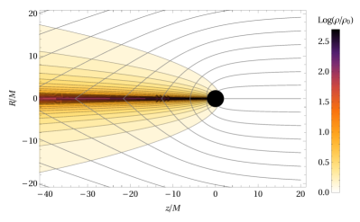
Figure 3: Analytic model of a relativistic wind accreting at $v_{\infty}=0.5$ onto a Schwarzschild black hole. Accretion flow streamlines are represented as gray, solid lines, while colour contours correspond to the density field level set.

In Figure 4 we compare the resulting streamlines in Schwarzschild spacetime with those coming from the Newtonian BHL model for different values of the asymptotic wind speed. From this figure it is clear that the accretion cylinder, and thus the total accretion rate, in the relativistic model is greater than the corresponding Newtonian value. In the next subsection we discuss this in further detail.

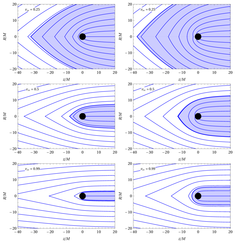
Figure 4: Comparison of the ballistic streamlines as obtained in the BHL model (left-hand column) and in Schwarzschild spacetime (right-hand column). The shaded area in each panel corresponds to the accretion cylinder, i.e. to those streamlines with impact parameter $b$ less than the critical value $b_{c}$ that end up accreting onto the central object. The wind speed at infinity $v_{\infty}$ is indicated at the top left of each panel.

3.4 Accretion rate

Just as for the density field, the procedure described in Section 2 to compute the total accretion rate in the Newtonian case (BHL model) is not as simple to implement for the relativistic problem. However, the logic behind this calculation remains the same: when the collision of mirror-reflected streamlines along the symmetry axis $(\theta=\pi)$ occurs, the flow’s kinetic energy associated to the normal component of the velocity ($U^{\theta}$ in this case) is lost from the system as thermal energy and/or radiation. The remaining relativistic energy $\mathcal{E}^{\prime}$ of a given streamline with impact parameter $b$ will determine whether the gas traveling along the streamline is accreted ($\mathcal{E}^{\prime}<1$) onto the central black hole or lost to infinity ($\mathcal{E}^{\prime}>1$). The streamline that is left marginally bound with $\mathcal{E}^{\prime}=1$ is characterized by the critical impact parameter $b_{c}$. Using the normalization condition $U_{\mu}U^{\mu}=-1$, together with $U^{\theta}=0$ and Eq. (3.2), it is simple to show that the condition $\mathcal{E}^{\prime}=1$ is equivalent to

$$r(\pi)^{3}+[2M-r(\pi)]\,b_{c}^{2}=0.$$ (3.24)

Unfortunately, after substituting $r(\pi)$ from either Eqs. (3.9) or (3.13), the resulting equation is highly non-linear in $b_{c}$ and it does not seem possible to solve it for $b_{c}$ explicitly. Nonetheless, it is straightforward to solve Eq. (3.24) numerically using a root-finding algorithm. We have done this using the bisection method for 1000 values of $v_{\infty}$ uniformly distributed between 0.001 and 0.999 to a precision of 10^-8. Now, based on these numerically calculated values, we found the following fit that approximates $b_{c}$ to an accuracy better than $3\%$ for $v_{\infty}<0.999$ and to within $0.5\%$ for $v_{\infty}<0.98$:

$$b_{c}^{\mathrm{fit}}=\frac{2M}{v^{2}_{\infty}}\left(1+c_{1}\,v_{\infty}+c_{2}\,v^{2}_{\infty}+c_{3}\,v^{3}_{\infty}\right),$$ (3.25)

with $c_{1}=0.081135$, $c_{2}=3.452826$ and $c_{3}=-1.758438$.

All of the streamlines within the cylinder $b\leq b_{c}$ contribute to the total accretion rate. According to the right-hand side of Eq. (3.22), we can therefore express $\dot{M}$ as

$$\dot{M}=\pi\,b_{c}^{2}\,\rho_{\infty}v_{\infty}\gamma_{\infty}.$$ (3.26)

In Figure 5 we show the resulting accretion rate as a function of the wind speed at infinity and compare it to the Newtonian value found in the BHL model (Eq. 2.7). As can be seen from this figure, the relativistic accretion rate is greater than the corresponding BHL one for all values of $v_{\infty}$, with the difference being more than double for $v_{\infty}\gtrsim 0.4$ and more than ten times larger for $v_{\infty}\gtrsim 0.8$. As expected, the relativistic accretion rate converges to the Newtonian value in the non-relativistic limit, i.e for $v_{\infty}\ll 1$. Contrary to the Newtonian case in which the accretion rate was a monotonically decreasing function of $v_{\infty}$, the relativistic result has an inflection point at around $v_{\infty}\simeq 0.8$ and becomes arbitrarily large as $v_{\infty}\rightarrow 1$. The culprit behind this behaviour is the special relativistic effect of Lorentz contraction that compresses the fluid volume elements along the direction of the wind and is represented by the Lorentz factor in Eq. (3.26).

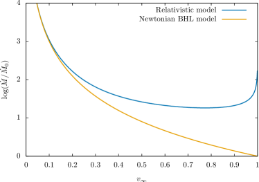
Figure 5: Mass accretion rate as a function of the wind speed at infinity $v_{\infty}$. The blue line corresponds to the (fitted) relativistic model as given by Eq. 3.25, while the yellow line corresponds to the Newtonian BHL model (Eq. 2.7). In both cases the accretion rate is expressed in units of $\dot{M}_{0}=4\pi M^{2}\rho_{\infty}$.

4 Comparison with numerical simulations

In this section we compare the analytic wind accretion model presented in the previous section against numerical hydrodynamic simulations performed with aztekas, a free GNU Public Licensed (GPL) code for solving any conservative set of equations, in particular, relativistic (with a non-trivial fixed metric) and non-relativistic hydrodynamic equations. Some aspects of aztekas, together with numerical and convergence tests relevant to the present work are discussed in the Appendix A. Further details and tests of the aztekas code will be presented elsewhere.

For all of the simulations discussed in this work, we considered a perfect fluid evolving on top a fixed Schwarzschild background metric described in terms of the horizon-penetrating, Kerr-Schild coordinates. Since the problem under study presents axial symmetry, all of the simulations were performed in 2D using polar coordinates $r$ and $\theta$. All of the results presented below were obtained after the numerical simulations had evolved in time from a uniform initial state condition until a relaxed stationary state was reached.

The relativistic hydrodynamic equations consist on the continuity equation (3.19) together with the local conservation of energy-momentum

$$\nabla_{\mu}T^{\mu\nu}=0,$$ (4.1)

where we take the energy-momentum tensor $T^{\mu\nu}$ corresponding to a perfect fluid (Landau & Lifshitz, 1975)

$$T^{\mu\nu}=\rho\,h\,U^{\mu}U^{\nu}+p\,g^{\mu\nu},$$ (4.2)

with rest mass density $\rho$, pressure $p$, specific internal energy $\epsilon$ and specific enthalpy $h=1+\epsilon+p/\rho$. Moreover, we adopt a Bondi-Wheeler equation of state (Tooper, 1965) of the form

$$\epsilon=\frac{p}{\rho\left(\Gamma-1\right)},$$ (4.3)

where $\Gamma$ is the polytropic index.

In order to integrate numerically Eqs. (3.19) and (4.1) with aztekas, we recast them in a conservative form based on the 3+1 formalism (see e.g. Font, 2000; Alcubierre, 2008), as follows

$$\frac{1}{\sqrt{-g}}\frac{\partial\left(\sqrt{\gamma}\,\mathbf{Q}\right)}{\partial t}+\frac{1}{\sqrt{-g}}\frac{\partial\left(\sqrt{-g}\,\mathbf{F}^{i}\right)}{\partial x^{i}}=\mathbf{S},$$ (4.4)

where $\gamma$ and $g$ are the determinants of the spatial 3-metric $\gamma_{ij}$ and the spacetime 4-metric $g_{\mu\nu}$, respectively. $\mathbf{Q}$ is the conservative variable vector, $\mathbf{F}^{i}=\left\{\mathbf{F}^{r},\mathbf{F}^{\theta}\right\}$ are the fluxes along the $r$ and $\theta$ coordinates and $\mathbf{S}$ is the source vector. All of these quantities depend on the primitive variables $\mathbf{U}$. The functional form of these vectors are presented below:

$$\mathbf{U}=\left[\rho,\ v_{j},\ p\right]^{T},$$ (4.5)

$$\mathbf{Q}=\left[D,\ S_{j},\ \tau\right]=\left[\rho W,\ \rho\,h\,W^{2}v_{j},\ \rho\,h\,W^{2}-p-D\right]^{T},$$ (4.6)

$$\begin{split}\mathbf{F}^{i}=\bigg{[}D\left(v^{i}-\frac{\beta^{i}}{\alpha}\right),\ &S_{j}\left(v^{i}-\frac{\beta^{i}}{\alpha}\right)+p\,\delta_{j}^{i},\\ &\left.\tau\left(v^{i}-\frac{\beta^{i}}{\alpha}\right)+p\,v^{i}\right]^{T},\end{split}$$ (4.7)

$$\begin{split}\mathbf{S}=\bigg{[}0,\ &T^{\mu\nu}\left(\frac{\partial g_{\nu j}}{\partial x^{\mu}}-\Gamma_{\nu\mu}^{\sigma}g_{\sigma j}\right),\\ &\left.\alpha\left(T^{\mu 0}\frac{\partial\ln\alpha}{\partial x^{\mu}}-T^{\mu\nu}\Gamma_{\nu\mu}^{0}\right)\right]^{T},\end{split}$$ (4.8)

where $\Gamma_{\mu\nu}^{\lambda}$ are the usual Christoffel symbols, $v^{i}$ is the three-velocity as measured by local Eulerian observers, $W=\left(1-\gamma_{ij}v^{i}v^{j}\right)^{-1/2}$ is the associated Lorentz factor, and

$$\alpha=\left(1+\frac{2M}{r}\right)^{-1/2},$$ (4.9)

$$\beta^{i}=\left(\frac{2M}{r}\left(1+\frac{2M}{r}\right)^{-1},\ 0\ ,\ 0\right),$$ (4.10)

are the lapse function and the shift vector, respectively, and correspond to the 3+1 decomposition of Schwarzschild spacetime in Kerr-Schild coordinates.

For the numerical flux calculation, we use in aztekas a high resolution shock capturing method (HRSC) with an HLLE approximate Riemann solver (Harten et al., 1983), combined with a monotonically centered (MC) second order reconstructor at cell interfaces. For the time integration, we use a second order Runge-Kutta method of lines in the total variation diminishing (TVD) version (Shu & Osher, 1988). Finally, we adopt a constant time-step defined through the CFL condition $\Delta t=C\,\min\left(\Delta r,r\,\Delta\theta\right)$, with $C=0.1$.

For the relativistic wind simulations, we ran two sets of simulations exploring asymptotic wind speeds from $v_{\infty}=0.1$ to $0.9$ for two different polytropic indices: $\Gamma=4/3$ and $5/3$. We took as numerical domain $[r_{\mathrm{min}},\ r_{\mathrm{max}}]\times[0,\pi]$, with $r_{\mathrm{min}}=0.5\,r_{\mathrm{acc}}$, $r_{\mathrm{max}}=10\,r_{\mathrm{acc}}$ and

$$r_{\mathrm{acc}}=\frac{M}{v_{\infty}^{2}+a_{\infty}^{2}},$$ (4.11)

where $a_{\infty}$ is the asymptotic speed of sound. The radius $r_{\mathrm{acc}}$ is commonly used in the literature (cf. Font et al., 1999; Cruz-Osorio et al., 2012), as a good estimate for the extension of the numerical domain necessary for numerical convergence. Our choice of this numerical domain is based on the convergence and resolution tests discussed in detail in the Appendix A.

For most of these simulations we used a fixed Mach number $\mathcal{M}=v_{\infty}/a_{\infty}=5$ in order to ensure that we were considering the same supersonic conditions in all cases. As a sanity check, we also considered $\mathcal{M}=10$ for a reduced number of cases. We used a uniform grid of $400\times 400$ cells except for the cases $v_{\infty}=0.1$, $0.8$ and $0.9$, where we had to use a larger grid of $1000\times 1000$ in order to find converged solutions.

As external boundary condition at the sphere $r=r_{\mathrm{max}}$, we enforced a constant, uniform inflow from the northern hemisphere $\theta\in[0,\pi/2)$ and free outflow from the southern one $\theta\in[\pi/2,\pi]$. As internal boundary condition, we set free outflow across the sphere at $r=r_{\mathrm{min}}$. The incoming wind at the external boundary has uniform thermodynamical variables $\rho_{\infty}$ and $p_{\infty}$. We set $\rho_{\infty}=10^{-10}$ in arbitrary units and take $p_{\infty}$ consistent with the chosen Mach number $\mathcal{M}$ and the equation of state, as in Cruz-Osorio et al. (2012):

$$p_{\infty}=\frac{a_{\infty}^{2}\rho_{\infty}(\Gamma-1)}{\Gamma(\Gamma-1)-a_{\infty}^{2}\Gamma}.$$ (4.12)

For the velocity field, we set an incoming wind with a constant velocity $\sqrt{v_{i}\,v^{i}}=v_{\infty}$, and components:

$$v_{r}=-\sqrt{g_{rr}}\,v_{\infty}\cos\theta,$$ (4.13)

$$v_{\theta}=\sqrt{g_{\theta\theta}}\,v_{\infty}\sin\theta,$$ (4.14)

where $g_{rr}$ and $g_{\theta\theta}$ are the radial and polar components of the metric respectively. As for the initial conditions of the simulation, we set them equal to the constant boundary values over all the numerical domain.

The simulations were left to run until a stationary state was reached. This was monitored by keeping track of the mass accretion rate, which was computed on the fly by integrating the relativistic radial mass flux across a control sphere of radius $r$ according to (Petrich et al., 1989)

$$\dot{M}=2\pi\int_{0}^{\pi}D\left(v^{r}-\frac{\beta^{r}}{\alpha}\right)\,r^{2}\sin\theta\mathrm{d}\theta.$$ (4.15)

It is important to remark that, once the stationary state is reached across all the numerical domain, the mass accretion rate as calculated from Eq. (4.15) has to have a constant value (to within numerical precision) independently of where the control radius $r$ is located (see Figure 12).

The typical simulation time at which steady state was reached depends on the wind velocity at infinity and the domain extension roughly as $t_{c}\approx r_{\mathrm{acc}}/v_{\infty}$. As an example, in Figure 6 we show the mass accretion rate as a function of time for $v_{\infty}=0.5$ and $\Gamma=4/3,\ 5/3$, measuring it at the event horizon $r=2M$.

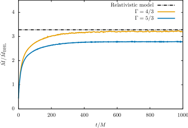
Figure 6: Mass accretion rate as a function of time for two wind simulations with asymptotic velocity $v_{\infty}=0.5$ and $\Gamma=4/3,\ 5/3$. As a reference, the horizontal dashed line shows the corresponding value from the relativistic model (Eq. 3.26). The stationary state is reached after $t\approx 600M$. The mass accretion rate has been scaled using the BHL result $\dot{M}_{\mathrm{BHL}}=4\pi M^{2}\rho_{\infty}/v_{\infty}^{3}$ (Eq. 2.7).

In Figure 7, we show the steady-state of the density field and streamlines of a wind accretion flow with $v_{\infty}=0.5$ and polytropic index $\Gamma=4/3$ on the left side panel and $\Gamma=5/3$ on the right side panel. As expected for a supersonic flow, a bow shock is formed downstream around the accretor, with a smaller shock cone for $\Gamma=4/3$ than for $\Gamma=5/3$.

In Figure 8, we compare the streamlines as obtained from the two simulations discussed in the previous paragraph against the ones from the analytic model. As can be seen from this figure, the ballistic approximation provides a qualitatively good description of the resulting streamlines upstream of the flow and in the region outside the bow shock, while inside the shock cone the streamline behavior is notably different.

We can also notice from both Figure 6 and Figure 8, that there is a better agreement between the analytic model and the $\Gamma=4/3$ case than for the $\Gamma=5/3$ one. This is related to the fact that the relative degree of incompressibility or stiffness of a polytropic fluid is directly proportional to the adiabatic index and, thus, a $\Gamma=5/3$ fluid resists more effectively the compression due to the gravitational field of the central object (geodesic focusing) than a fluid with $\Gamma=4/3$.

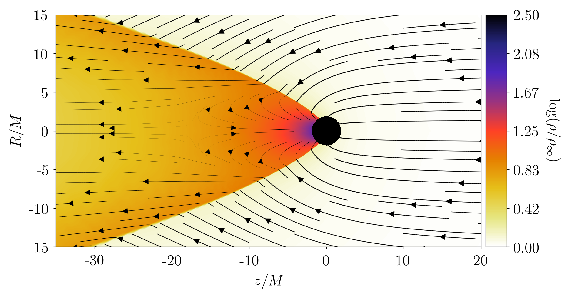
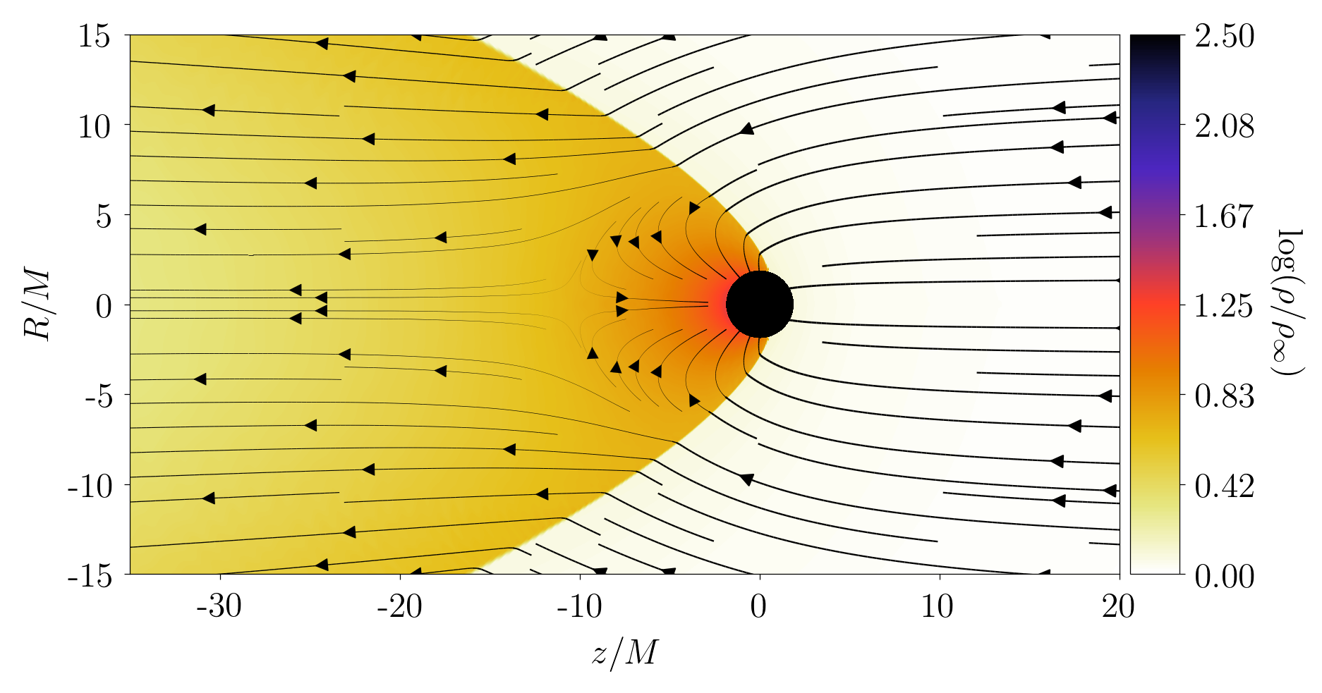
Figure 7: Numerical simulations performed with aztekas of a relativistic wind accreting onto a Schwarzschild black hole. The chosen polytropic index is $\Gamma=4/3$ for the left side panel and $\Gamma=5/3$ for the right side one, while the asymptotic wind velocity is $v_{\infty}=0.5$. The plot shows the stationary-state streamlines and in colour isocontour levels of the corresponding density field. The width of the streamlines is proportional to the velocity magnitude $v=\sqrt{v_{i}\,v^{i}}$.

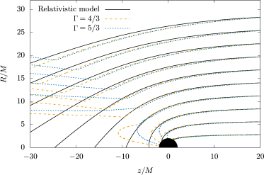
Figure 8: Comparison of the streamlines of the analytic model against the corresponding ones extracted from the numerical simulations for $v_{\infty}=0.5$, $\mathcal{M}=5$ and $\Gamma=4/3,\ 5/3$.

In order to compare the numerical mass accretion rate with the ballistic model (Eq. 3.24), we computed the mean value of Eq. (4.15) across all the radial domain. In Figure 9 we show the comparison between the analytic model presented in the previous section and the simulations for both $\Gamma=4/3$ and $5/3$.

Moreover, we also explored the dependence of the mass accretion rate on the Mach number by performing 10 additional simulations with $\mathcal{M}=10$. In Figure 9, the square marks show the mass accretion rate for these simulations. Note that these results overlay with the $\mathcal{M}=5$ cases (the relative difference between both results is less than $0.7\%$). The resulting bow shocks are also very similar in both cases, with slightly smaller cones for the $\mathcal{M}=10$ case.

As can be seen in Figure 9, the resulting accretion rate from the numerical simulations is consistently slightly larger for the $\Gamma=4/3$ simulations than for the $\Gamma=5/3$ ones. Moreover, a good agreement is found between the accretion rate as predicted by the relativistic model and the one obtained from the aztekas simulations, with a relative error less than 10% for all of the 28 simulations presented in this work.

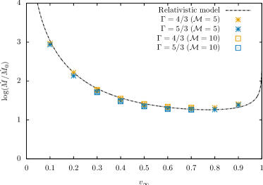
Figure 9: Comparison of the mass accretion rate as obtained from the relativistic model (Eq. 3.26) versus the numerical values obtained from the aztekas simulations. The colour marks show the results of the 28 simulations discussed in this work for asymptotic wind speeds $v_{\infty}=0.1,\,0.2,\ldots,0.9$, two polytropic indices $\Gamma=4/3,\,5/3$, and two Mach numbers $\mathcal{M}=5,\,10$. The mass accretion rate is expressed in units of $\dot{M}_{0}=4\pi M^{2}\rho_{\infty}$.

5 Summary

We have presented a full relativistic, analytic model of a supersonic wind accreting onto a Schwarzschild black hole. In addition to the assumptions of stationarity and axisymmetry, the model is based on the ballistic approximation in which the streamlines of the accretion flow correspond to geodesic trajectories of a Schwarzschild spacetime. Following the methodology presented in Tejeda et al. (2012), the streamlines of the model were described analytically in terms of Jacobi elliptic functions. The density field of the resulting accretion flow and the corresponding accretion rate were calculated using simple numerical schemes.

The model presented in this paper constitutes the relativistic generalisation of the Newtonian wind accretion model by Bondi-Hoyle-Lyttleton (BHL). Naturally, the relativistic model recovers the BHL model in the non-relativistic limit $v_{\infty}\ll\mathrm{c}$. The enhanced gravitational field of the accreting object in general relativity, together with the special relativistic effect of Lorentz contraction, contribute to a larger accretion rate as compared to that of the BHL model (see Figure 5). This difference becomes substantial (by a factor of 10-100) for asymptotic wind speeds $v_{\infty}$ close to the speed of light c. Although these large velocities are not expected to be common in astrophysical settings, they can appear in extreme cases such as the velocity kick imparted onto a newborn black hole following an asymmetrical supernova explosion (Janka, 2013) or after the merger of two rotating black holes (Gerosa & Moore, 2016).

We have compared the new relativistic model against numerical simulations performed with the aztekas code. This code solves numerically the full hydrodynamic evolution of a perfect fluid in Schwarzschild spacetime starting off from a uniform condition until a stationary state is reached. We have used two different polytropic equations of state ($\Gamma=4/3$ and $\Gamma=5/3$) and asymptotic wind speeds from $v_{\infty}=0.1\,\mathrm{c}$ to $v_{\infty}=0.9\,\mathrm{c}$. We have considered two different values for the asymptotic Mach number, $\mathcal{M}=5$ and 10, finding virtually no difference between these two values. We have found a good agreement (to within 10%) between the accretion rate predicted by the relativistic model and the aztekas simulations (see Figure 9). As expected for these supersonic flows, the ballistic streamlines of the analytic model agree quite well with the resulting streamlines of the numerical simulations in the upwind region outside the bow shock.

6 Acknowledgements

We thank Sergio Mendoza, Alejandro Cruz-Osorio, Olivier Sarbach and Francisco S. Guzmán for useful discussions and comments on the manuscript. We also thank the anonymous referee for helpful suggestions and remarks. This work was supported by DGAPA-UNAM (IN112616 and IN112019) and CONACyT (CB-2014-01 No. 240512; No. 290941; No. 291113) grants.

Appendix A Validation of the numerical hydrodynamic code aztekas

In this Appendix we present several numerical tests intended to validate our use of aztekas in this work.

A.1 Spherical accretion

In order to test aztekas in the general relativistic hydrodynamic regime, it is important to compare with a benchmark solution. For this, we employ the analytic model of spherical accretion developed by Michel (1972).

In Figure 10, we compare the outcome of numerical simulations performed with aztekas against Michel’s analytic solution for the same values of polytropic index used in the wind accretion problem ($\Gamma=4/3,5/3$) and for an asymptotic sound speed of $a_{\infty}=0.01$.

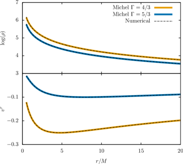
Figure 10: Comparison of the numerical hydrodynamic simulations performed with aztekas against the relativistic spherical accretion model of Michel (1972). The top panel shows the density as a function of radius while the bottom panel shows the radial velocity for two different values of the polytropic index $\Gamma=4/3,\ 5/3$ and an asymptotic sound speed of $a_{\infty}=0.01$.

For these simulations, we took a 2D spherical axisymmetric grid of $400\times 400$ uniformly distributed radial bins $r\in\left[0.5M,20M\right]$ and polar bins $\theta\in\left[0,\pi/2\right]$. We set the boundary conditions at $r=20M$ by imposing Michel’s solution there. As initial conditions we populate the entire numerical domain with the boundary constant value and let the system evolve until a stationary regime is reached for $t\gtrsim 100M$. As can be seen from Figure 10, an excellent agreement is found between Michel’s analytic solution and the aztekas simulation results. We compute the mass accretion rate and the relative error between both solutions is below 0.2%.

Also using this benchmark solution, we looked at the convergence rate of aztekas by computing the $L^{1}$ norm of the density error for different numerical resolutions $N_{r}$, i.e.

$$L^{1}(\rho_{\mathrm{num}},\rho_{\mathrm{exact}})=\frac{1}{N_{r}}\sum_{i=1}^{N_{r}}|\rho_{\mathrm{num}}(r_{i})-\rho_{\mathrm{exact}}(r_{i})|,$$ (A.1)

where $\rho_{\mathrm{num}}$ and $\rho_{\mathrm{exact}}$ are the numerical and exact values of the density, respectively. In Figure 11, we show the result of this test from where we obtain a convergence rate consistent with a second order, which is to be expected for smooth solutions and for our use of the MC reconstructor.

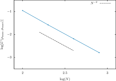
Figure 11: $L^{1}$ norm of the density error for the Michel test, using resolutions $N_{r}=100,\,200,\,400\,\mathrm{and}\,800$. The dashed line shows the slope that corresponds to a second order convergence rate.

A.2 Dependence on domain extension and resolution

We also want to make sure that the numerical solutions obtained with aztekas have converged to physical values and that the results are independent from both numerical resolution and domain extension.

Due to the finite extension of the numerical domain $r_{\mathrm{max}}$, the total accretion rate calculated from the numerical simulations shows a small dependence on $r_{\mathrm{max}}$ that gets weaker as larger domain extensions are considered. For example, in Figure 12 we show the resulting mass accretion rate for simulations with $v_{\infty}=0.5$, $\Gamma=5/3$ and seven different domain extensions, at $t=1000M$. As can be seen from this figure, our choice of a domain extension of $r_{\mathrm{max}}=10\,r_{\mathrm{acc}}$ leads to an overestimation of the mass accretion rate of the order of $\sim 5\%$, which is an acceptable margin of error for us in this work. We expect the rest of the simulations to behave in a similar way.

Similarly, we also looked at this same domain extension dependence but now by monitoring the mass accretion rate across a fixed radius (in this case across the event horizon at $r=2M$) as a function of time. As can be seen from Figure 13, the difference between a domain extension of $10\,r_{\mathrm{acc}}$ and of $25\,r_{\mathrm{acc}}$ maintains the same margin error of $\sim 5\%$ along time.

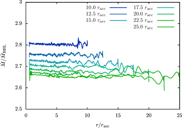
Figure 12: Comparison of the mass accretion rate for different domain extensions. In all cases $v_{\infty}=0.5$, $\Gamma=5/3$, and the simulation time is $t=1000M$.

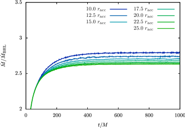
Figure 13: Same as in Figure 12, but now measuring the mass accretion rate across $r=2M$ as a function of time.

In what regards the numerical resolution, we found that the grid size does not affect as directly the value of the resulting accretion rate. However, it does contribute to the smoothness of the solution, with larger resolutions leading to less numerical noise. In Figure 14 we show an example of this again for the case $v_{\infty}=0.5$, $\Gamma=5/3$ and five different numerical resolutions: $\mathcal{R}_{1}=200\times 200$, $\mathcal{R}_{2}=300\times 300$, $\mathcal{R}_{3}=400\times 400$, $\mathcal{R}_{4}=500\times 500$ and $\mathcal{R}_{5}=600\times 600$. As discussed in the Section 4, for most of the simulations presented in this work we settled for $\mathcal{R}_{3}$ as a good compromise between accuracy and performance.

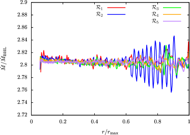
Figure 14: Comparison between the mass accretion rate for different resolutions $\mathcal{R}_{1}=200\times 200$, $\mathcal{R}_{2}=300\times 300$, $\mathcal{R}_{3}=400\times 400$, $\mathcal{R}_{4}=500\times 500$ and $\mathcal{R}_{5}=600\times 600$, for $v_{\infty}=0.5$, $\Gamma=5/3$ and $t=1000M$.

Finally, in order to estimate the convergence rate of the simulations, and given that there is no analytical solution for the full hydrodynamic wind accretion, we follow Lora-Clavijo & Guzmán (2013) and measure the self-convergence rate using different resolutions. To this purpose, we ran two sets of three simulations each, with resolutions

$$\mathcal{R}_{1}=200\times 200,\,\mathcal{R}_{2}=300\times 300\text{ and }\mathcal{R}_{3}=450\times 450,$$

and

$$\mathcal{R}_{1}=200\times 200,\,\mathcal{R}_{2}=400\times 400\text{ and }\mathcal{R}_{3}=800\times 800.$$

Note that, for each set separately, there is a factor of $k=1.5$ and $k=2$ between successive resolutions. With the simulation results at hand, we compute the self-convergence factor $Q$ according to

$$k^{Q}=\frac{L^{1}(\rho_{1},\rho_{2})}{L^{1}(\rho_{2},\rho_{3})},$$ (A.2)

with $L^{1}(\rho_{i},\rho_{j})$ as defined in Eq. (A.1) and where $\rho_{1}$, $\rho_{2}$ and $\rho_{3}$ are the densities along the accretion axis $(\theta=\pi)$ for each of the employed resolutions. The results for this test are shown in Figure 15. As can be seen from this figure, for both set of resolutions we find an order of convergence between 1.5 and 2 in the steady state region, which is to be expected for this kind of algorithms due to the presence of shocks.

Figure 15: Self-convergence of the wind simulations (see Eq. A.2) for two sets of simulations with a ratio of $k=1.5$ and $2$ between successive resolutions. In both cases the convergence rate $Q$ stays between 1.5 and 2 in the steady state region, as required for this test due to the presence of shocks.

References

- Aguayo-Ortiz et al. (2018) Aguayo-Ortiz A., Mendoza S., Olvera D., 2018, PLoS ONE, 13, e0195494
- Alcubierre (2008) Alcubierre M., 2008, Introduction to 3+1 Numerical Relativity. Oxford University Press
- Bisnovatyi-Kogan et al. (1979) Bisnovatyi-Kogan G. S., Kazhdan I. M., Klypin A. A., Lutskii A. E., Shakura N. I., 1979, Astronomicheskii Zhurnal, 56, 359
- Bondi (1952) Bondi H., 1952, Monthly Notices of the Royal Astronomical Society, 112, 195+
- Bondi & Hoyle (1944) Bondi H., Hoyle F., 1944, Monthly Notices of the Royal Astronomical Society, 104, 273
- Cruz-Osorio & Lora-Clavijo (2016) Cruz-Osorio A., Lora-Clavijo F. D., 2016, Monthly Notices of the Royal Astronomical Society, 460, 3193
- Cruz-Osorio et al. (2012) Cruz-Osorio A., Lora-Clavijo F. D., Guzmán F. S., 2012, MNRAS, 426, 732
- Cruz-Osorio et al. (2017) Cruz-Osorio A., Sánchez-Salcedo F. J., Lora-Clavijo F. D., 2017, Monthly Notices of the Royal Astronomical Society, 471, 3127
- Edgar (2004) Edgar R., 2004, New Astronomy Review, 48, 843
- El Mellah & Casse (2015) El Mellah I., Casse F., 2015, Monthly Notices of the Royal Astronomical Society, 454, 2657
- El Mellah et al. (2018) El Mellah I., Sundqvist J. O., Keppens R., 2018, Monthly Notices of the Royal Astronomical Society, 475, 3240
- Font (2000) Font J. A., 2000, Living Reviews in Relativity, 3, 2
- Font & Ibáñez (1998) Font J. A., Ibáñez J. M., 1998, Astrophysical Journal, 494, 297
- Font et al. (1999) Font J. A., Ibáñez J. M., Papadopoulos P., 1999, MNRAS, 305, 920
- Frank et al. (2002) Frank J., King A., Raine D., 2002, Accretion Power in Astrophysics, 3rd edn. Cambridge University Press
- Frolov & Novikov (1998) Frolov V. P., Novikov I. D., 1998, Black Hole Physics: Basic Concepts and New Developments. Kluwer Academic
- Gerosa & Moore (2016) Gerosa D., Moore C. J., 2016, Physical Review Letters, 117, 011101
- Gracia-Linares & Guzmán (2015) Gracia-Linares M., Guzmán F. S., 2015, Astrophysical Journal, 812, 23
- Harten et al. (1983) Harten A., Lax P. D., Leer B., 1983, SIAM Review, 25
- Hoyle & Lyttleton (1939) Hoyle F., Lyttleton A., 1939, Mathematical Proceedings of the Cambridge Philosophical Society, 35, 405
- Hunt (1971) Hunt R., 1971, Monthly Notices of the Royal Astronomical Society, 154, 141
- Janka (2013) Janka H.-T., 2013, Monthly Notices of the Royal Astronomical Society, 434, 1355
- Landau & Lifshitz (1975) Landau L., Lifshitz E., 1975, The Classical Theory of Fields, 4th ed. edn. Vol. 2 of Course of Theoretical Physics, Pergamon
- Lawden (1989) Lawden D. F., 1989, Elliptic Functions and Applications. Springer
- Longair (2011) Longair M. S., 2011, High Energy Astrophysics
- Lora-Clavijo & Guzmán (2013) Lora-Clavijo F. D., Guzmán F. S., 2013, Monthly Notices of the Royal Astronomical Society, 429, 3144
- Mendoza et al. (2009) Mendoza S., Tejeda E., Nagel E., 2009, Monthly Notices of the Royal Astronomical Society, 393, 579
- Michel (1972) Michel F. C., 1972, Astrophysics and Space Science, 15, 153
- Olvera & Mendoza (2008) Olvera D., Mendoza S., 2008, in Oscoz A., Mediavilla E., Serra-Ricart M., eds, EAS Publications Series Vol. 30 of EAS Publications Series, A GPL Relativistic Hydrodynamical Code. pp 399–400
- Petrich et al. (1989) Petrich L. I., Shapiro S. L., Stark R. F., Teukolsky S. A., 1989, Astrophysical Journal, 336, 313
- Petrich et al. (1988) Petrich L. I., Shapiro S. L., Teukolsky S. A., 1988, Physical Review Letters, 60, 1781
- Romero & Vila (2014) Romero G. E., Vila G. S., eds, 2014, Introduction to Black Hole Astrophysics Vol. 876 of Lecture Notes in Physics, Berlin Springer Verlag
- Ruffert & Arnett (1994) Ruffert M., Arnett D., 1994, Astrophysical Journal, 427, 351
- Schroven et al. (2017) Schroven K., Hackmann E., Lämmerzahl C., 2017, Physical Review D, 96, 063015
- Shima et al. (1985) Shima E., Matsuda T., Takeda H., Sawada K., 1985, Monthly Notices of the Royal Astronomical Society, 217, 367
- Shu & Osher (1988) Shu C.-W., Osher S., 1988, Journal of Computational Physics, 77, 439
- Tejeda (2018) Tejeda E., 2018, Revista Mexicana de Astronomía y Astrofísica, 54, 171
- Tejeda et al. (2012) Tejeda E., Mendoza S., Miller J. C., 2012, Monthly Notices of the Royal Astronomical Society, 419, 1431
- Tejeda et al. (2013) Tejeda E., Taylor P. A., Miller J. C., 2013, Monthly Notices of the Royal Astronomical Society, 429, 925
- Tooper (1965) Tooper R. F., 1965, ApJ, 142, 1541
- Zanotti et al. (2011) Zanotti O., Roedig C., Rezzolla L., Del Zanna L., 2011, Monthly Notices of the Royal Astronomical Society, 417, 2899