ADI/ACA-like Superfast Iterative Refinement of
Low Rank Approximation of a Matrix

Abstract

We call a matrix algorithm superfast (aka running at sublinear cost) if it involves much fewer flops and memory cells than an input matrix has entries. Computations with Big Data frequently involve matrices of immense size and can be reduced to computations with low rank approximations (LRA) of these matrices, which can be performed superfast. Unfortunately, such LRA algorithms fail for worst case input matrices admitting their LRAs, but Adaptive Cross-Approximation (ACA) method, which can be viewed as LRA version of Alternative Directions Implicit (ADI) method, is highly efficient empirically for LRA of a large and important class of input matrices. Adequate formal support for that empirical behavior, however, is still a challenge. This motivated us to propose a novel ADI/ACA-like superfast randomized iterative refinement of a crude LRA. Like ACA iterations we output CUR LRA, which is a particularly memory efficient form of LRA. Unlike ADI/ACA method we use sampling probability to reduce our task to recursive solution of generalized Linear Least Squares Problem (generalized LLSP) and to prove monotone convergence to a close LRA with a high probability (whp) under mild assumptions on an initial LRA. For crude initial LRA lying reasonably far from optimal we have consistently observed significant improvement in two or three iterations in our numerical tests .

Keywords:

Superfast (sublinear cost) algorithms, Low rank approximation, CUR LRA, Linear least square problem, Johnson and Lindenstrauss lemma, Iterative refinement, Adaptive Cross-approximation, ADI method

2020 Math. Subject Classification:

65Y20, 65F05, 65F55, 68Q25, 68W20, 68W25

1 Introduction

1.1. Superfast LRA: background and our progress. Low Rank Approximation (LRA) of a matrix is among the most fundamental subjects of Numerical Linear Algebra and Data Mining and Analysis, with applications ranging from PDEs to machine learning theory, neural networks, term document data, and DNA SNP data (see [19, 15, 29], and the bibliography therein). Quite typically $m\times n$ matrices $M$ representing Big Data (e.g., unfolding matrices of multidimensional tensors) are so immense that one must apply superfast (aka sublinear cost) algorithms, using much fewer than $mn$ flops, e.g., operating with LRA of a matrix $M$ whenever such an LRA is available.

Unfortunately, one cannot compute superfast an LRA of worst case inputs and not even of $mn+1$ matrices of our Example 2.1. This example, however, does not apply to refinement of a crude initial LRA, and for this task we devise, analyze and test a superfast iterative algorithm. The algorithm is similar to Adaptive Cross-Approximation (ACA) iterations (cf. [2]) and like them can be considered an LRA version of Alternative Directions Implicit (ADI) method (cf. [18, 3]).

ACA iterations, celebrated for their empirical efficiency, output CUR LRA, a particularly memory efficient LRA, traced to [13, 12] and generated by a matrix $G$ of a small size. ACA iterations are directed towards computing such a germ $G$ by means of maximization of its volume $|\det(G^{*}G)|^{1/2}$ (see [12, 2, 23] and the references therein).

We also output CUR LRA, but our approach is different. Instead of volume maximization we use random sampling directed by sampling probabilities of [7] and, unlike the case of ACA iterations, formally prove monotone convergence of our iterative refinement whp under mild assumptions on an initial LRA. In our tests for initial LRAs lying reasonably far from optimal, our iterative refinement has consistently yielded significant improvement already in a few iterations.

1.2. Some technical details and related works. As in [7], we reduce LRA to the solution of generalized LLSP by applying to an input matrix $M$ random sampling defined by sampling probabilities. [7] computes nearly optimal LRA whp and does this superfast, except for the stage of computing sampling probabilities. In every iteration of our refinement we compute them superfast as well because we only need them for low rank matrices. Our refinement algorithm combines such a superfast variant of random sampling of [7] and superfast ADI/ACA-like iterations and inherits superfast performance and numerical stability of both ACA and random sampling of [7]. There only remained the non-trivial challenge of proving that our iterative refinement of a crude LRA monotone converges whp; we succeeded based on estimating the principal angle distances between subspaces associated with singular vectors and computed recursively in our refinement process.

As in [7], we formally support our algorithm by sampling fairly many rows and columns of an input matrix, but sampling a much fewer rows or columns was sufficient in numerical tests with real world data in both [7] and our Sec. 6.3.

The report [10] proposed a distinct and more primitive iterative refinement of LRA. It relies on recursive application of a superfast sub-algorithm for LRA given as a part of an input, while we assume no sub-algorithm available and unlike [10] use randomization techniques of [7].

The paper [16] also uses ADI/ACA-like iterations and principal angle distances. Unlike us, however, it studies completion of a coherent matrix with exact rank $r$, rather than LRA. Furthermore, it relies on uniform element-wise sampling.

Superfast algorithms of [4, 17, 21] compute LRAs of Symmetric Positive Semi-definite matrices and Distance matrices but not of general ones; their techniques are different from ours.

1.3. Organization of the paper. We devote the next section and Appendices A and B to background. In Sec. 3 we cover a generic algorithm for iterative refinement of LRA by means of recursive solution of generalized LLSP at superlinear cost. In Sec. 4 we recall subspace sampling algorithms of [7], directed by leverage scores. In Sec. 5 we cover randomized iterative refinement of a crude but sufficiently close LRA, leaving one of the proofs to Appendix C. In Sec. 6 we cover the results of our numerical experiments. We devote Sec. 7 to conclusions.

2 Background for LRA

2.1. $r$-top SVD, matrix norms, pseudo inverse, and Principal Angle Distance. For simplicity we assume dealing with real matrices in $\mathbb{R}^{p\times q}$ throughout.

$r$-top SVD of a matrix $M$ of a rank at least $r$ is the decomposition $M_{r}=U^{(r)}\Sigma^{(r)}V^{(r)T}$ for the diagonal matrix $\Sigma^{(r)}=\operatorname{diag}(\sigma_{j})_{j=1}^{r}$ of the $r$ largest singular values of $M$ and for two orthogonal matrices $U^{(r)}$ and $V^{(r)}$ of the associated top left and right singular spaces, respectively.

$M_{r}$ is said to be the $r$-truncation of $M$ and is unique if there is a gap between the $r$th and $(r+1)$st largest singular values, i.e., if $\sigma_{r}(M)>\sigma_{r+1}(M)$.

$M_{r}=M$ for a matrix $M$ of rank $r$, and then its $r$-top SVD is just its compact SVD

$$M=U_{M}\Sigma_{M}V^{T}_{M},\leavevmode\nobreak\ {\rm for}\leavevmode\nobreak\ U_{M}=U^{(r)},\leavevmode\nobreak\ \Sigma_{M}=\Sigma^{(r)},\leavevmode\nobreak\ {\rm and}\leavevmode\nobreak\ V_{M}=V^{(r)}.$$

$M^{+}:=V_{M}\Sigma_{M}^{-1}U^{T}_{M}$ is the Moore–Penrose pseudo inverse of $M$.

$||M||$ and $||M||_{F}$ denote the spectral and Frobenius norms of $M$, respectively, such that $||M||:=\sigma_{1}(M)$ and $||M||_{F}^{2}:=\sum_{j=1}^{\min\{m,n\}}\sigma_{j}^{2}$.

By following [15] we use unified notation $|||\cdot|||$ for both of these matrix norms.

Lemma 2.1.

[The norm of the pseudo inverse of a matrix product.] Suppose that $A\in\mathbb{R}^{k\times r}$, $B\in\mathbb{R}^{r\times l},$ and the matrices $A$ and $B$ have full rank $r\leq\min\{k,l\}$. Then $|||(AB)^{+}|||\leq|||A^{+}|||\leavevmode\nobreak\ |||B^{+}|||$.

Definition 2.1.

[16]. Let $E_{1}$ and $E_{2}$ be two subspaces of $\mathbb{R}^{m}$, and let $G$, $G_{\perp}$, $H$, and $H_{\perp}$ be matrices with orthonormal columns that generate subspaces $E_{1}$, $(E_{1})_{\perp}$, $E_{2}$, and $(E_{2})_{\perp}$, respectively. Define the Principal Angle Distance between $E_{1}$ and $E_{2}$:

$$\operatorname*{Dist}(E_{1},E_{2})=||G_{\perp}^{T}H||=||H_{\perp}^{T}G||.$$ (2.1)

Remark 2.1.

Let $E_{1}$ and $E_{2}$ be two linear subspaces of $\mathbb{R}^{m}$. Then

(i) $\operatorname*{Dist}(E_{1},E_{2})$ ranges from 0 to 1,

(ii) $\operatorname*{Dist}(E_{1},E_{2})=0$ if and only if $\textrm{Span}(E_{1})=\textrm{Span}(E_{2})$, and

(iii) $\operatorname*{Dist}(E_{1},E_{2})=1$ if $\textrm{rank}(E_{1})\neq\textrm{rank}(E_{2})$.

2.2. $\epsilon$-rank, LRA, and optimal LRA. A matrix $M$ has $\epsilon$-rank at most $r$ if it admits approximation within an error norm $\epsilon$ by a matrix $M^{\prime}$ of rank at most $r$ or equivalently if there exist four matrices $A$, $B$, $M^{\prime}$, and $E$ such that

$$M=M^{\prime}+E,\leavevmode\nobreak\ |||E|||\leq\epsilon\leavevmode\nobreak\ |||M|||,\leavevmode\nobreak\ M^{\prime}=AB,\leavevmode\nobreak\ A\in\mathbb{R}^{m\times r},\leavevmode\nobreak\ {\rm and}\leavevmode\nobreak\ B\in\mathbb{R}^{r\times n}.$$ (2.2)

$\epsilon$-rank $\rho$ of a matrix $M$ is numerically unstable if $\rho$-th and $(\rho+1)$-st or $\rho$-th and $(\rho-1)$-st largest singular values of $M$ are close to one another, but it is quite commonly used in numerical matrix computations (cf. [9, pages 275-276]), and we can say that a matrix admits LRA if it has $\epsilon$-rank $r$ where $r$ and $\epsilon$ are small in context.

Theorem 2.1.

The Eckart-Young-Mirsky theorem: LRA by means of truncation of SVD (see [25, 8, 22], [9, Thm. 2.4.8]. The matrix $M_{r}$, the $r$-truncation of SVD of $M$, is optimal rank-$r$ approximation of $M$ under both spectral and Frobenius norms:

$$|||M_{r}-M|||=\min_{X:\leavevmode\nobreak\ \operatorname{rank}(X)=r}|||X-M|||,$$ (2.3)

$||M_{r}-M||=\sigma_{r+1}(M)$ and $||M_{r}-M||_{F}=\sigma_{F,r+1}(M):=\sqrt{\sum_{j>r}\sigma_{j}^{2}(M)}$.

Example 2.1.

A small family of hard input matrices for superfast LRA. Fill an $m\times n$ matrix $\Delta_{i,j}$ with 0s except for its $(i,j)$th entry filled with 1. Expand the family $\Delta:=\{\Delta_{i,j},\leavevmode\nobreak\ i=1,\dots,m;\leavevmode\nobreak\ j=$ $1,\dots,n\}$ of all $mn$ such matrices of rank 1 with the $m\times n$ null matrix $O_{m,n}$. A superfast algorithm, e.g., a superfast a posteriori error estimator, does not access the $(i,j)$th entry of its input matrices for some pair of $i$ and $j$ or misses such an entry with a positive constant probability if it is randomized. Hence it fails with an undetected error at least 1/2 at this entry on both the family $\Delta\cup\{O_{m,n}\}$ and its perturbation by a fixed matrix $M\in\mathbb{R}^{m\times n}$ of low rank.

2.3. CUR LRA.  For $M\in\mathbb{R}^{m\times n}$ and two sets $\mathcal{I}\subseteq\{1,\dots,m\}$ and $\mathcal{J}\subseteq\{1,\dots,n\}$ define the submatrices $M_{\mathcal{I},:}:=(m_{i,j})_{i\in\mathcal{I};j=1,\dots,n}$, $M_{:,\mathcal{J}}:=(m_{i,j})_{i=1,\dots,m;j\in\mathcal{J}}$, and $G:=M_{\mathcal{I},\mathcal{J}}:=(m_{i,j})_{i\in\mathcal{I};j\in\mathcal{J}}$, define canonical rank-$r$ CUR approximation of $M$:

$$M\approx M^{\prime}=CUR,\leavevmode\nobreak\ C=M_{:,\mathcal{J}},\leavevmode\nobreak\ U=G^{-1},\leavevmode\nobreak\ {\rm and}\leavevmode\nobreak\ R=M_{\mathcal{I},:},$$ (2.4)

and call the matrices $G$ and $U$ its generator and nucleus, respectively. Call $M^{\prime}$ a CUR LRA of $M$ if $|||M^{\prime}-M^{\prime}|||$ and $r$ are small in context. For $G\in\mathbb{R}^{k\times l}$ computation of CUR LRA only involves $kl$ memory cells and $O((k+l)kl)$ flops.

Remark 2.2.

More generally, the nucleus $U$ can be any matrix in $\mathbb{R}^{l\times k}$; the Frobenius error norm is minimized for $U=C^{+}MR^{+}$ (see [27, Sec. 4],[20, Eqn. (6)]): $||E||_{F}=||M-CUR||_{F}\leq||M-CC^{+}M||_{F}+||M-MR^{+}R||_{F}$. We cannot compute the nucleus $U=C^{+}MR^{+}$ superfast, however.

3 Generic iterative refinement of LRA

Definition 3.1.

Generalized Linear Least Squares Problem (LLSP):
Given two matrices $M\in\mathbb{R}^{m\times n}$ and $A\in\mathbb{R}^{m\times r}$, compute $Y:=\operatorname*{arg\,min}_{X}||M-AX||_{F}.$

Algorithm 3.1.

Generic refinement via recursive solution of generalized LLSPs, see Fig. 1.

Input:

$M\in\mathbb{R}^{m\times n}$, $A_{0}\in\mathbb{R}^{m\times r}$, and $B_{0}\in\mathbb{R}^{r\times n}$ such that $0<r\leq\min\{m,n\}$,

$$M\approx A_{0}B_{0},\leavevmode\nobreak\ \sigma_{r}(M)>\sigma_{r+1}(M),\textrm{ and}\leavevmode\nobreak\ \operatorname*{Dist}(U^{(r)},A_{0})<1.$$

Initialization:

Fix a (reasonably large) integer $T$.

Computations:

Recursively compute

$$B_{t+1}:=A_{t}^{+}M\textrm{ and }A_{t+1}:=MB_{t+1}^{+},\leavevmode\nobreak\ t=0,1,\dots,T.$$

Output:

Matrices $A_{T}$ and $B_{T}$.

One can prove that $\operatorname*{Dist}(M,A_{T}B_{T})\rightarrow 0$ as $T\rightarrow\infty$, but the algorithm is not superfast: the matrices $A_{t}^{+}$ and $B_{t}^{+}$ are dense even where the matrices $A_{0}$ and $B_{0}$ are sparse. Moreover, the output LRA is not CUR LRA. Both of our algorithm and ACA iterations fix these deficiencies.

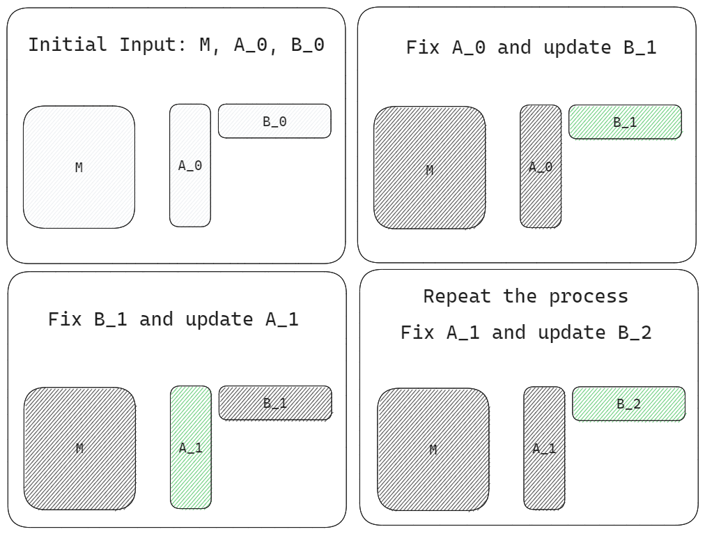
Figure 1: Alternating Refinement

4 Generalized LLSP and CUR LRA computation with random sampling directed by leverage scores: the State of the Art

4.1 Rank-$r$ leverage scores: definition

Definition 4.1.

(See [7].) Given an ${m\times n}$ matrix $M$ with $\sigma_{r}(M)>\sigma_{r+1}(M)$, and its $r$-top SVD $M_{r}=U^{(r)}\Sigma^{(r)}V^{(r)T}$, write

$$\gamma_{i}:=\sum_{j=1}^{r}v_{i,j}^{2},\leavevmode\nobreak\ \textrm{ for }i=1,\dots,n,\leavevmode\nobreak\ {\rm and}\leavevmode\nobreak\$$ (4.1)

$$\tilde{\gamma}_{i}:=\sum_{j=1}^{r}u_{i,j}^{2},\leavevmode\nobreak\ \textrm{ for }i=1,\dots,m,$$ (4.2)

where $v_{i,j}$ and $u_{i,j}$ denote the $(i,j)$-th entry of matrices $V^{(r)}$ and $U^{(r)}$ respectively. Then call $\gamma_{i}$ and $\tilde{\gamma}_{i}$ the rank-$r$ Column and Row Leverage Scores of $M$, respectively.

Remark 4.1.

The $r$-top left and right singular spaces of $M$ are uniquely defined if $\sigma_{r}(M)>\sigma_{r+1}(M)$.

Remark 4.2.

The row/column leverage scores define probability distributions because $\sum_{i=1}^{m}\tilde{\gamma}_{i}=\sum_{i=1}^{n}\gamma_{i}=r$. By following [7] we allow soft probability distributions $\{p_{i}|i=1,\dots,n\}$ and $\{\tilde{p}_{i}|i=1,\dots,m\}$: given $\{\gamma_{i}|i=1,\dots,n\}$ and $\{\tilde{p}_{i}|i=1,\dots,m\}$, fix $\beta$, $0<\beta\leq 1$, allow to increase sampling size by a factor of $\beta^{-1}$, and only require that

$$p_{i}>0,\leavevmode\nobreak\ p_{i}\geq\beta\gamma_{i}/r\leavevmode\nobreak\ {\rm for}\leavevmode\nobreak\ i=1,\dots,n,\leavevmode\nobreak\ {\rm and}\leavevmode\nobreak\ \sum_{i=1}^{n}p_{i}=1,$$ (4.3)

$$\tilde{p}_{i}>0,\leavevmode\nobreak\ \tilde{p}_{i}\geq\beta\tilde{\gamma}_{i}/r\leavevmode\nobreak\ {\rm for}\leavevmode\nobreak\ i=1,\dots,m,\leavevmode\nobreak\ \sum_{i=1}^{m}\tilde{p}_{i}=1,$$ (4.4)

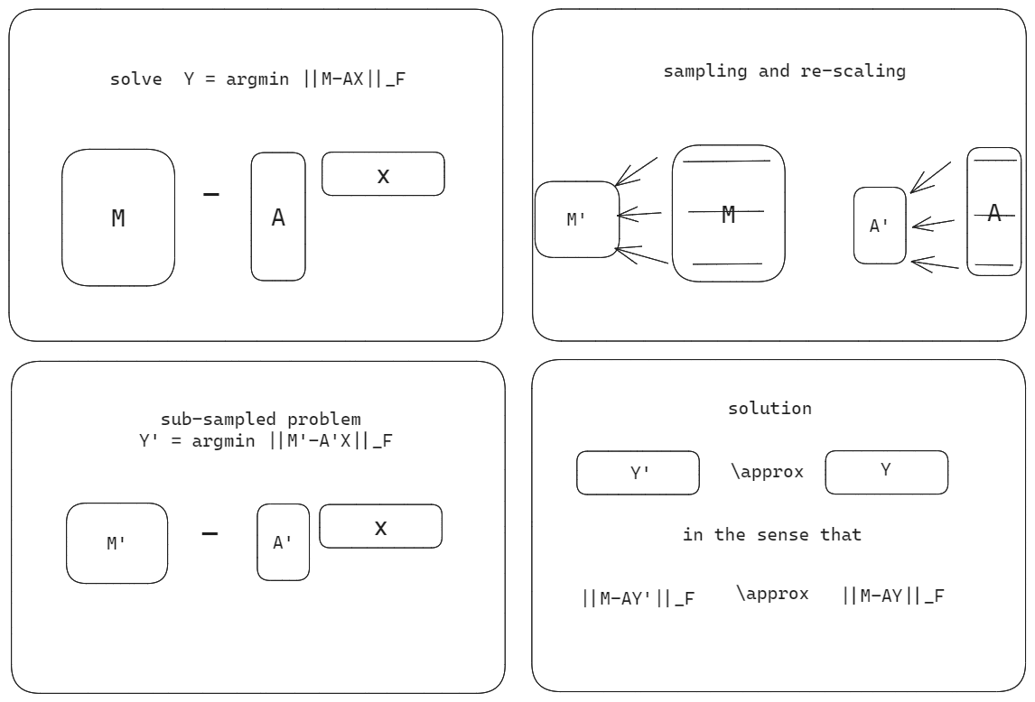
Figure 2: Solving LLSP through Sampling

Theorem 4.1 (Adapted from Thm. 5 of [7]).

Let $\tilde{\gamma}_{i}$ for $i=1,\dots,m$ be the rank-$r$ row leverage scores of a rank-$r$ matrix $A\in\mathbb{R}^{m\times r}$ and let $M\in\mathbb{R}^{m\times n}$. Fix three positive numbers $\epsilon<1$, $\xi<1$, and $\beta\leq 1$ and compute probability distribution $\{\tilde{p}_{i}|i=1,\dots,m\}$ satisfying relationships (4.4). Write $l:=1296\beta^{-1}r^{2}\epsilon^{-2}\xi^{-4}$ and let $S$ and $D$ be the sampling and scaling matrices output by Alg. A.1. Then (see Fig. 2)

$$\textrm{rank}(D^{T}S^{T}A)=r\hskip 14.22636pt\textrm{and}\hskip 14.22636pt||A\tilde{X}-M||_{F}\leq(1+\epsilon)||AA^{+}M-M||_{F}$$ (4.5)

with a probability no less than $1-\xi$ where

$$\tilde{X}:=(D^{T}S^{T}A)^{+}D^{T}S^{T}M.$$ (4.6)

Thm. 4.1 says that we can solve generalized LLSP superfast if we are given leverage scores of [7] with $l=1296\beta^{-1}r^{2}\epsilon^{-2}\xi^{-4}\ll m$, but according to numerical tests in both our section 6.3 and [7] much smaller row samples are often sufficient.

4.2 Rank-$r$ leverage scores: perturbation

The following result implies that the $r$-top singular space and hence the leverages scores are stable in a small norm perturbation of a matrix $M$ (cf. [7, Thm. 5].)

Theorem 4.2.

(Adapted from [26, Thm. 6.4], [11, Thm. 1].) Suppose that

$$M=\begin{bmatrix}U_{r}&U_{\perp}\end{bmatrix}\begin{bmatrix}\Sigma_{r}&\\ &\Sigma_{\perp}\end{bmatrix}\begin{bmatrix}V_{r}^{T}\\ V_{\perp}^{T}\end{bmatrix}$$

is SVD, $g=:\sigma_{r}(M)-\sigma_{r+1}(M)-2\leavevmode\nobreak\ ||E||>0$, and $||E||_{F}<\frac{g}{2}$. Then there exist matrices $P\in\mathbb{R}^{(m-r)\times r}$ and $Q\in\mathbb{R}^{(n-r)\times r}$ such that

$$||[P^{T},Q^{T}]||_{F}<2\frac{||E||_{F}}{g}<1$$

and the columns of the matrices $U^{(r)}+U_{\perp}P$ and $V^{(r)}+V_{\perp}Q$ span the $r$-top left and right singular spaces of $M+E$.

Remark 4.3.

Unlike $U^{(r)}+U_{\perp}P$ and $V^{(r)}+V_{\perp}Q$, the matrices

$$\widetilde{U^{(r)}}=(U^{(r)}+U_{\perp}P)(I_{r}+P^{T}P)^{-\frac{1}{2}}\leavevmode\nobreak\ \textrm{ and }\leavevmode\nobreak\ \widetilde{V^{(r)}}=(V^{(r)}+V_{\perp}Q)(I_{r}+Q^{T}Q)^{-\frac{1}{2}}$$

have orthonormal columns. Let $\gamma_{i}$ and $\tilde{\gamma}_{i}$ denote the rank-$r$ leverage scores of the $i$-th row of $M$ and $M+E$, respectively, defined by the squared row norms of $U^{(r)}$ and $\widetilde{U^{(r)}}$, respectively. Then

$$\frac{1}{1+||P||^{2}}\leavevmode\nobreak\ \Big{(}1-\frac{||P||}{\sqrt{\gamma_{i}}}\Big{)}^{2}\leq\tilde{\gamma}_{i}/\gamma_{i}\leq\Big{(}1+\frac{||P||}{\sqrt{\gamma_{i}}}\Big{)}^{2}\leavevmode\nobreak\ {\rm for}\leavevmode\nobreak\ \gamma_{i}\neq 0,\leavevmode\nobreak\ \leavevmode\nobreak\ i=1,2,3,\dots,m,$$

and $||P||=O(||E||_{F})$ if the perturbation $E$ satisfies the assumption of Thm. 4.2. The ratio of column leverage scores satisfies similar bounds.

5 Superfast randomized iterative refinement of LRA by means of refinement of leverage scores

Outline of iterative refinement of LRA: Next we combine Alg. 3.1 with random sampling of [7], recalled in the previous section. Given a low rank matrix (e.g., a crude LRA of an input matrix output by the algorithms of [24]), refine it as follows: at a dominated cost compute top SVD of LRA, leverage scores, and by using them a new LRA of an input matrix. If this refines the original LRA, apply the computation recursively. At every recursive step refine just one of the two factors $A$ and $B$ of an LRA $AB$ and compute the second factor superfast whp by solving a generalized LLSP. Given a matrix $A_{0}\in\mathbb{R}^{m\times r}$, first compute a matrix $B_{0}\in\mathbb{R}^{r\times n}$ such that $A_{0}B_{0}$ is a crude but reasonably close approximation of an input matrix $M\in\mathbb{R}^{m\times n}$ (assume that there exists such a matrix $B_{0}$); then successively compute matrices $A_{1}$, $B_{1}$, $A_{2}$, $B_{2}$, $\dots$ such that the values $\operatorname*{Dist}(A_{t},U^{(r)})$ and $\operatorname*{Dist}(B_{t},V^{(r)})$ converge with a controllable error bound as $t\rightarrow\infty$, where $U^{(r)}$ and $V^{(r)}$ denote two orthogonal matrices whose range (column span) defines the $r$-top left and right singular spaces of $M$, respectively.

Algorithm 5.1.

[Alternating Refinement Using Leverage Scores.]

Input:

A matrix $M\in\mathbb{R}^{m\times n}$, a positive integer $\tau$, a target rank $r$, positive real numbers $\epsilon$ and $\xi<1$, and matrices $A_{0}\in\mathbb{R}^{m\times r}$ and $B_{0}\in\mathbb{R}^{r\times n}$.

Computations:

FOR $t=0,1,\dots,\tau-1$ DO:

1. Compute the row leverage scores $\tilde{\gamma}_{i}$ of $A_{t}$, fix an appropriate $0<\beta\leq 1$, and compute probabilities $\tilde{p}_{i}$ satisfying (4.4) for $i=1,\dots,m$.

2. Apply Alg. A.1 to matrices $M$ and $A_{t}$ for $l=1296\beta^{-1}r^{2}\epsilon^{-2}\xi^{-4}$ to compute sampling and scaling matrices $S$ and $D$.

3. Compute $B_{t+1}=(D^{T}S^{T}A_{t})^{+}D^{T}S^{T}M$.

4. Compute the column leverage scores $\gamma_{i}$ of $B_{t+1}$, fix an appropriate $0<\beta\leq 1$, and compute probabilities $p_{i}$ satisfying (4.3) for $i=1,\dots,n$.

5. Apply Alg. A.1 to matrices $M$ and $B_{t+1}$ for $l=1296\beta^{-1}r^{2}\epsilon^{-2}\xi^{-4}$ to compute sampling and scaling matrices $S$ and $D$.

6. Compute $A_{t+1}=MSD(B_{t+1}SD)^{+}$.

END FOR

Output:

$A_{\tau}$ and $B_{\tau}$.

Theorem 5.1.

Let $M$ be an $m\times n$ matrix such that $\sigma_{r}(M)>\sigma_{r+1}(M)$, and let

$$M=\begin{bmatrix}U^{(r)}&U_{\perp}\end{bmatrix}\begin{bmatrix}\Sigma^{(r)}&\\ &\Sigma_{\perp}\end{bmatrix}\begin{bmatrix}V^{(r)T}\\ V_{\perp}^{T}\end{bmatrix}$$

be SVD. Let $A$ be an $m\times r$ orthogonal matrix with $r\leq\min\{m,n\}$ such that

$$\operatorname*{Dist}(A,U^{(r)})=\delta<1.$$ (5.1)

Fix positive numbers $\epsilon<1$, $\xi<1$, and $\beta\leq 1$ and compute the rank-$r$ row leverage scores $\{\gamma_{i}|i=1,\dots,m\}$ of $A$ and a sampling distribution $\{p_{i}|i=1,\dots,m\}$ satisfying (4.4). Suppose that Alg. A.1, applied for $l=1296\beta^{-1}r^{2}\epsilon^{-2}\xi^{-4}$, outputs two matrices $S$ and $D$. Write $B:=(D^{T}S^{T}A)^{+}D^{T}S^{T}M$. Then

$$\operatorname*{Dist}(B,V^{(r)})\leq\frac{\delta}{\sqrt{1-\delta^{2}}}\cdot\frac{\sigma_{r+1}(M)}{\sigma_{r}(M)}+\frac{2\epsilon}{\sqrt{1-\delta^{2}}}\cdot\frac{\sigma_{F,r+1}(M)}{\sigma_{r}(M)}$$ (5.2)

with a probability no less than $1-\xi$.

Proof.

See Appendix C. ∎

To simplify notation write $\sigma_{j}:=\sigma_{j}(M)$ for $j=1,2,3,\dots,r$ and $\bar{\sigma}_{r+1}:=\sigma_{F,r+1}(M)=||M-M_{r}||_{F}$.

Lemma 5.1.

Let $m,n,r,\epsilon,\delta$, $M$, $U^{(r)}$, $V^{(r)}$, $A$ and $B$ be defined as in Thm. 5.1 such that $A$ and $B$ satisfy (5.1) and (5.2). Then $\operatorname*{Dist}(B,V^{(r)})\leq c\cdot\operatorname*{Dist}(A,U^{(r)})$ for

$$c=\frac{\sigma_{r+1}}{\sigma_{r}}\cdot\frac{1}{\sqrt{1-\delta^{2}}}\cdot(1+2\epsilon\cdot\frac{\bar{\sigma}_{r+1}}{\delta\sigma_{r+1}}).$$

Furthermore, if $\frac{\sigma_{r+1}}{\sigma_{r}}\cdot\frac{1}{\sqrt{1-\delta^{2}}}<1$ and $\epsilon\cdot\frac{\bar{\sigma}_{r+1}}{\sigma_{r+1}}<\frac{\delta}{2}\big{(}\sqrt{1-\delta^{2}}\frac{\sigma_{r}}{\sigma_{r+1}}-1\big{)}$, then $c<1$.

If $\operatorname*{Dist}(B_{t},V^{(r)})<c\cdot\operatorname*{Dist}(A_{t},U^{(r)})$, $\operatorname*{Dist}(A_{t+1},U^{(r)})<c\cdot\operatorname*{Dist}(B_{t},V^{(r)})$ for $t\leq\tau$, and $0<c<1$, then the principal angle distance is reduced by a constant factor $1/c>1$ each time when we compute $B_{t}$ for a given $A_{t}$ or compute $A_{t+1}$ for a given $B_{t}$. We ensure that $1/c>1$ provided that there is a gap between $\sigma_{r}$ and $\sigma_{r+1}$ and that the initial factor $A$ is reasonably close to $U^{(r)}$ in terms of the principal angle distance.

The second term of the bound (5.2) comes from the error contributed by the perturbation $M-M_{r}$ and does not converge to zero even if we perform our recursive refinement indefinitely. We, however, are going to decrease the principal angle distance to a value of the order of $\nu:=\epsilon\cdot\frac{\bar{\sigma}_{r+1}}{\sigma_{r+1}}$ where we can decrease a positive $\epsilon$ at will, although we need order of $\log(\nu)$ refinement iterations to decrease the principal angle distance between $A$ and $U^{(r)}$ below $\nu$ whp, under some reasonable assumptions about an input matrix $M$ and a starting factor $A:=A_{0}$.

Theorem 5.2.

Suppose that $m,n,r$, $M$, $U^{(r)}$, $V^{(r)}$ are defined as in Thm. 5.1,

$$\frac{\sigma_{r+1}(M)}{\sigma_{r}(M)}\leq\frac{1}{2},\leavevmode\nobreak\ A_{0}\in\mathbb{R}^{m\times r},\leavevmode\nobreak\ {\rm and}\leavevmode\nobreak\ \operatorname*{Dist}(A_{0},U^{(r)})\leq\frac{1}{2}.$$

Write

$$\theta:=\frac{\bar{\sigma}_{r+1}}{\sigma_{r+1}},\leavevmode\nobreak\ {\rm so\leavevmode\nobreak\ that}\leavevmode\nobreak\ 1\leq\theta^{2}\leq\min\{m,n\}-r,$$

fix two sufficiently small positive numbers $\xi$ and $\epsilon$ such that

$$\xi<1\leavevmode\nobreak\ {\rm and}\leavevmode\nobreak\ \epsilon\leq(8\theta)^{-1}\leq 1/2,$$

and let $A$ denote the matrix output by Alg. 5.1 applied for $\tau=\lceil\frac{1}{2}\log_{0.87}(8\theta\cdot\epsilon)\rceil$. Then

$$\operatorname*{Dist}(A,U^{(r)})\leq 4\theta\cdot\epsilon$$ (5.3)

with a probability no less than $1-2\tau\cdot\xi$.

Proof.

If $\delta=\delta_{t}:=\operatorname*{Dist}(A_{t},U^{(r)})\leq 1/2$, then

$$\frac{1}{\sqrt{1-\delta^{2}}}\frac{\sigma_{r+1}}{\sigma_{r}}\leq\frac{1}{\sqrt{3}}.$$

Furthermore, (5.2) implies that

$$\operatorname*{Dist}(B_{t},V^{(r)}) \leq\frac{\delta}{\sqrt{1-\delta^{2}}}\cdot\frac{\sigma_{r+1}}{\sigma_{r}}+\frac{2\epsilon}{\sqrt{1-\delta^{2}}}\cdot\frac{\sigma_{r+1}}{\sigma_{r}}\cdot\frac{\bar{\sigma}_{r+1}}{\sigma_{r+1}}$$

$$\leq\frac{1}{\sqrt{3}}\cdot\delta+\frac{2\theta}{\sqrt{3}}\cdot\epsilon.$$

Thus it can be readily verified that

$$\operatorname*{Dist}(B_{t},V^{(r)})\leq 3\delta/2\sqrt{3}<0.87\cdot\operatorname*{Dist}(A_{t},U^{(r)})\hskip 5.69046pt\leavevmode\nobreak\ {\rm if}\leavevmode\nobreak\ \delta\geq 4\theta\cdot\epsilon$$

and that

$$\operatorname*{Dist}(B_{t},V^{(r)})\leq 6\theta\cdot\epsilon/\sqrt{3}<4\theta\cdot\epsilon\hskip 5.69046pt\leavevmode\nobreak\ {\rm if}\leavevmode\nobreak\ \delta<4\theta\cdot\epsilon.$$

Now let $\operatorname*{Dist}(A_{0},U^{(r)})\leq 1/2$. Then $\operatorname*{Dist}(B_{t},V^{(r)})\leq 0.87\cdot\operatorname*{Dist}(A_{t},U^{(r)})$ whp for every $t\geq 0$ and such that $\operatorname*{Dist}(A_{t},U^{(r)})\geq 4\theta\cdot\epsilon$. We prove this claim by applying Thm. 5.1 for $B_{t}^{T}$ and $M^{T}$ and noticing that the bound $\operatorname*{Dist}(A_{t},U^{(r)})\leq 1/2$ is maintained throughout our algorithm.

By combining these results, obtain for all $t$ such that $\operatorname*{Dist}(A_{t},U^{(r)})\leq 1/2$ that

$$\operatorname*{Dist}(A_{t+1},U^{(r)})\leq\max\big{\{}(0.87)^{2}\operatorname*{Dist}(A_{t},U^{(r)}),4\theta\cdot\epsilon\big{\}}$$ (5.4)

with a probability no less than $1-2\xi$. Complete the proof of the theorem by recursively applying this bound for $t=0,\dots,\tau-1$. ∎

6 Numerical Tests

6.1 Overview

We implemented our algorithms in Python with Numpy and Scipy packages. For solving generalized LLSP we call lstsq and for computing Rank Revealing QR factorization we call qr, relying on Lapack function gelsd and dgeqp3, respectively.

We performed all tests on a machine running Mac OS 10.15.7 with 2.6 GHz Intel Core i7 CPU and 16GB of Memory.

6.2 Input matrices for LRA

We used the following classes of input matrices:

• A $3000\times 3000$ fast-decay matrix $U\Sigma V^{T}$ where $U$ and $V$ are the matrices of the left and right singular vectors of the SVD of a $3000\times 3000$ Gaussian random matrix, respectively, and where $\Sigma={\rm Diag}(\sigma_{i})_{i=1}^{3000}$ for $\sigma_{i}=1$ for $i\leq r$ and $\sigma_{i}=2^{-(i-r)}$ for $i>r$.

• A $3000\times 3000$ slow-decay matrix; it denotes the same product $U\Sigma V^{T}$ except that now we let $\sigma_{i}=1$ for $i\leq r$ and $\sigma_{i}=(1+i-r)^{-2}$ for $i>r$.

• A $3000\times 3000$ single-layer potential matrix; it discretizes a single-layer potential operator of [15, Sec. 7.1]

  $$[Sf](x)=\int_{\Gamma_{1}}\log|x-y|\cdot f\leavevmode\nobreak\ \textrm{d}\sigma(y),\leavevmode\nobreak\ x\in\Gamma_{2},$$

  for a constant $f$, for two curves $\Gamma_{1}(t)=\big{(}r(t)\cos(t),r(t)\sin(t)\big{)}$ and $\Gamma_{2}=(3\cos(t),3\sin(t))$ in $\mathbb{R}^{2}$, for $t\in[0,2\pi]$ and $r(t)=2.5+\cos(3t)$.

• A $2000\times 2000$ Cauchy matrix $(\frac{1}{X_{i}-Y_{j}})_{i,j=1}^{2000}$. Here $X_{i}$ and $Y_{j}$ denote independent random variables $X_{i}$ and $Y_{j}$ uniformly distributed on the intervals $(0,100)$ and $(100,200)$, respectively. This matrix has fast decaying singular values (cf. [3]).

• A $1000\times 1000$ shaw matrix. It discretizes a one-dimensional image restoration model.

  We set target rank $r$ to 11 in the case of the single layer potential matrix and set the rank to 10 for all other input matrices.

6.3 Iterative refinement directed by leverage scores

We computed an initial LRA (rank-$r$ approximation) of an input matrix $M$ in two ways:

(i) First apply the Range Finder ([15, Alg. 4.1]) to compute an orthonormal matrix $Q$; then output LRA $QQ^{T}M$.

(ii) Apply a single APA loop to compute CUR LRA $CG^{-1}R$, where the generator matrix $G$ is an $r\times r$ submatrix of $M$ and $C$ and $R$ are corresponding column and row submatrices of $M$, respectively. Namely, first compute RRQR factorization of randomly selected column submatrix $C_{0}$; the resulting permutation matrix determines a row index set and a row submatrix $R$. Then compute RRQR factorization of the matrix $R$; the resulting permutation matrix determines a column index set and hence matrix $C$ and generator $G$.

In both cases (i) and (ii) we have only sought a crude initial LRA: namely, we applied [15, Alg. 4.1] (Range Finder) with only small oversampling in case (i) and applied just a small number of ACA steps in case (ii), leaving some room for refinement.

We applied Alg. 5.1 separately to the two initial approximations (i) and (ii) above. For each alternating refinement step we sampled $d$ columns or $d$ rows, for $d=15r$, which turned out to be sufficiently large in our tests, even though for our formal support of our refinement results we needed much larger samples of order $r^{2}\epsilon^{-2}$.

We computed the Frobenius relative error norm $\frac{||M-A_{i}B_{i}||_{F}}{||M-M_{r}||_{F}}$ for the initial LRA $A_{0}B_{0}$ and all LRAs $A_{i}B_{i}$ computed at the $i$th refinement steps for $i=1,2,3,4,5$.

We repeated the experiments 50 times and displayed the average error ratios in table 6.1.

	HMT11 + Refinement
Input	Init.	1st step	2nd step	3rd step	4th step	5th step
shaw	9.2486	1.3920	1.1726	1.0892	1.0727	1.0772
SLP	3.5421	1.4720	1.1462	1.0971	1.0912	1.0825
Cauchy	5.7180	1.4783	1.1383	1.0764	1.0826	1.0747
slow decay	3.1190	1.7194	1.0826	1.0726	1.0715	1.0680
fast decay	2.0612	1.6596	1.2429	1.1054	1.0756	1.0735
	Cross-Approximation + Refinement
Input	Init.	1st step	2nd step	3rd step	4th step	5th step
shaw	8.5939	1.0782	1.0723	1.0754	1.0674	1.0752
SLP	6.2216	1.4372	1.1017	1.0796	1.0764	1.0782
Cauchy	1703.7035	2.4336	1.1003	1.0829	1.0797	1.0773
slow decay	2.5236	1.1128	1.0691	1.0726	1.0710	1.0683
fast decay	2.0717	1.3539	1.1595	1.0898	1.0743	1.0752

Table 6.1: Reducing Error Ratio in Refinements Alg. 5.1

For both choices of the initial approximation, the tests show that already the first few steps Alg. 5.1 have significantly decreased the initial relative error norm, which has been more or less stabilized in the subsequent steps.

Recall that the algorithm of [15] (of case (i)) runs at linear cost of order $mn$ for an $m\times n$ input matrix $M$, while Alg. 5.1 and those of [13, 23] (of case (ii)) are superfast. Hence in case (i) we achieved significant improvement of a crude LRA at rather a nominal computational cost. In case (ii) our refinement cost is comparable with the cost of ACA initialization, and we consistently achieved significant improvement of an initial LRA already in two or three refinement steps.

6.4 Refinement of LRA with three options for solving generalized LLSP

In these tests we started with uniformly and randomly selected $r$ columns of $M$ and then performed alternating refinement of LRA by using three different LLSP algorithms: (a) sampling directed by leverage scores (Alg. 5.1), (b) subspace embedding with a Gaussian multiplier, and (c) the standard Linear Least Squares Solver.

(b) The subspace embedding with Gaussian multiplier is a well-known approximation approach, where in each iteration one computes $B_{i}=\operatorname*{arg\,min}_{X}||GA_{i}X-GM||_{F}$ and $A_{i+1}=\operatorname*{arg\,min}_{X}||XB_{i}H-MH||_{F}$ and where $G$ and $H$ are Gaussian matrices of size $d\times m$ and $n\times d$, respectively, generated independently.

(c) The standard Linear Least Squares Solver computes

$$\textstyle B_{i}=\operatorname*{arg\,min}_{X}||A_{i}X-M||_{F}\leavevmode\nobreak\ {\rm and}\leavevmode\nobreak\ A_{i+1}=\operatorname*{arg\,min}_{X}||XB_{i}-M||_{F};$$

this more costly algorithm outputs an optimal solution.

In each iteration we computed the average principal angle distance (between the matrices of the $r$-top left singular vectors of the input matrix and its approximation) and the average run time from 10 repeated tests, and plotted our tests results in Fig. 3. The tests showed that similarly to the relative error norm in the tests of the previous subsections, the principal angle distance also decreased significantly in the first few iterations and stabilized in the subsequent iterations.

The principal angle distance would have converged to 0 if the computations were exact and if the refinement process were done with the standard algorithm for the LLSP (case (c)), but the distance was still expected to converge to a small positive value if the approximation algorithms using Gaussian embedding (case (b)) or sampling directed by leverage scores (case (a)) were applied for LLSP. This small value can be controlled by the embedding dimension and the number of samples.

The tests confirm this expected behavior even in the presence of rounding errors: the refinement based on the standard LLSP solver decreased the principal angle distance considerably stronger than with the two other approaches, (a) and (b), whose output LRAs (and actually CUR LRAs, unlike the case of using the Standard Algorithm), however, were still close to optimal.

According to our tests for running time, in cases (a) and (b) the algorithms have run significantly faster than in case (c). Moreover, the algorithm with leverage scores (case (a)) used considerably less time at each iteration than the Gaussian Embedding approach (b), and this benefit strengthened as the size of the input matrix grew.

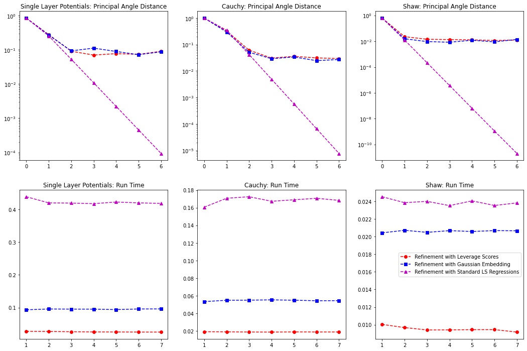
Figure 3: Principal Angle Distance with Least Squares Regression in Refinements Alg. 5.1

7 Conclusions

We devised and analyzed an ADI-like superfast algorithm for iterative refinement of an LRA and proved that it outputs a meaningful or even nearly optimal solution whp under randomization. Next we list some natural further challenges.

1. Devise and analyze other ADI-like superfast algorithms for iterative refinement of an LRA by using other recipes for random sampling, in particular the recipes that are friendly to Sparse input matrices (cf. [1, 6]).

2. Can we accelerate convergence of such iterative algorithms by combining them, e.g., by combining our and ACA iterations?

3. Find formal support for empirical observation that the outputs of our random sampling algorithms and those of [7] are accurate where only a reasonably small number of columns and rows is sampled.

Appendix

Appendix A Randomized Computation of Sampling and Scaling Matrices

Algorithm A.1.

([7, Alg. 4], The Exactly($l$) Sampling and Scaling.)

Input:

Two integers $l$ and $n$ such that $1\leq l\leq n$ and $n$ positive scalars $p_{1},\dots,p_{n}$ such that $\sum_{i=1}^{n}p_{i}=1$.

Initialization:

Let $S:=O_{n,l}$ and $D:=O_{l,l}$ be matrices filled with zeros.

Computations:

FOR $t=1,\dots,l$ DO

1. Generate an independent random integer $N$ from $\{1,\dots,n\}$ such that $\textrm{Prob}\{N=i\}=p_{i}$;

2. Set $s_{N,t}=1$, i.e., set the $N$-th element of the $t$-th column of $S$ to 1;

3. Set $d_{t,t}=1/\sqrt{lp_{N}}$;

END FOR

Output:

$n\times l$ sampling matrix $S=(s_{i,t})_{i,t=1}^{n,l}$ and $l\times l$ scaling matrix $D=\operatorname{diag}(d_{t,t})_{t=1}^{l}$.

Remark A.1.

Our next algorithm (Alg. A.2) reproduces Alg. 5 (Expected($l$)) from [7], and is an alternative to Alg. A.1. It computes random sampling and scaling matrices of randomly determined size, expected to be much smaller than in Alg. A.1. We simplify our presentation by only using Alg. A.1.

Algorithm A.2.

Expected($l$) Sampling and Scaling. [7, Alg. 5]).

Input:

same as in Alg. A.1.

Initialization:

Fix zero matrices $S$ and $D$ and integer $l=0$.

Computations:

FOR $j=1,\dots,n$ DO

1. Pick $j$ with the probability $\min\{1,lp_{j}\}$;

2. IF $j$ is picked THEN:

   • $l\leftarrow l+1$;

   • $s_{j,l}:=1$, i.e. set the $j$-th element of the $l$-th column of $S$ to 1;

   • $d_{l,l}:=1/\min\{1,\sqrt{lp_{j}}\}$;

   END IF

END FOR

Output:

$n\times l$ sampling matrix $S=(s_{i,j})_{i,j=1}^{n,l}$ and $l\times l$ scaling matrix $D=\operatorname{diag}(d_{i,i})_{i=1}^{l}$.

Alg. A.2 involves $nl$ memory cells and $O((l+1)n)$ flops and computes $l$ square roots. Here $l$ is a random number that depends on how many indices $j$ are picked in the process, and its expectation is $O(\epsilon^{-2}r\log r)$.

Appendix B Computation of CUR LRA directed by leverage scores

For completeness of our exposition we next recall the algorithms of [7], which reduce LRA of a matrix $M$ to solution of two generalized LLSPs by using random sampling (performed by means of Alg. A.1 or A.2) and which output CUR LRA of a matrix $M$ such that whp

$$||M-CUR||_{F}\leq(1+\epsilon)\sigma_{F,r+1}$$ (B.1)

for $\sigma_{F,r+1}$ of Thm. 2.1 and any fixed positive $\epsilon$. Let us supply some details.

Let $M_{r}=U^{(r)}\Sigma^{(r)}V^{(r)T}$ be $r$-top SVD and let scalars $\gamma_{1},\dots,\gamma_{n}$ be the rank-$r$ column leverage scores for the matrix $M$ (cf. (4.1)). They stay invariant if we pre-multiply the matrix $V^{(r)T}$ by an orthogonal matrix. Furthermore, for a fixed positive $\beta\leq 1$, we can compute a sampling probability distribution (4.3) at a dominated computational cost. For any $m\times n$ matrix $M$, [15, Alg. 5.1] computes the matrix $V^{(r)}$ and distribution $p_{1},\dots,p_{n}$ by using $mn$ memory cells and $O(mnr)$ flops, but the next algorithm, representing [7, Algs. 1 and 2], computes a CUR LRA of a matrix $M$ superfast except for the stage of computing leverage scores.

Algorithm B.1.

[CUR LRA by using leverage scores.]

Input:

A matrix $M\in\mathbb{R}^{m\times n}$ and a target rank $r$.

Initialization:

Choose two integers $k\geq r$ and $l\geq r$ and real $\beta$ and $\bar{\beta}$ in the range $(0,1]$.

Computations:

1. Compute the probability distribution $p_{1},\dots,p_{n}$ of (4.3).

2. Compute sampling and scaling matrices $S$ and $D$ by applying Alg. A.1 or A.2. Compute and output a CUR factor $C:=MS$.

3. Compute distribution $\bar{p}_{1},\dots,\bar{p}_{m}$ satisfying (4.3) under the following replacement: $M\leftarrow(CD)^{T}$ and $\beta\leftarrow\bar{\beta}$.

4. By applying Alg. A.1 or A.2 to the matrix $(CD)^{T}$ compute $k\times l$ sampling matrix $\bar{S}$ and $k\times k$ scaling matrix $\bar{D}$.

5. Compute and output a CUR factor $R:=\bar{S}^{T}M$.

6. Compute and output a CUR factor $U:=DW^{+}\bar{D}$ for $W:=\bar{D}\bar{S}^{T}MSD$.

Complexity estimates: Overall Alg. B.1 involves $kn+ml+kl$ memory cells and $O((m+k)l^{2}+kn)$ flops in addition to $mn$ cells and $O(mnr)$ flops used for computing SVD-based leverage scores at stage 1. Except for that stage the algorithm is superfast if $k+l^{2}\ll\min\{m,n\}$.

Bound (B.1) is expected to hold whp for the output of the algorithm if we choose integers $k$ and $l$ by combining [7, Thms. 4 and 5] as follows.

Theorem B.1.

Suppose that

(i) $M\in\mathbb{R}^{m\times n}$, $0<r\leq\min\{m,n\}$, $\epsilon,\beta,\bar{\beta}\in(0,1]$, and $\bar{c}$ is a sufficiently large constant,

(ii) four integers $k$, $k_{-}$, $l$, and $l_{-}$ satisfy the bounds

$$0<l_{-}=3200r^{2}/(\epsilon^{2}\beta)\leq l\leq n\leavevmode\nobreak\ {\rm and}\leavevmode\nobreak\ 0<k_{-}=3200l^{2}/(\epsilon^{2}\bar{\beta})\leq k\leq m$$ (B.2)

or

$$l_{-}=\bar{c}\leavevmode\nobreak\ r\log(r)/(\epsilon^{2}\beta)\leq l\leq n\leavevmode\nobreak\ {\rm and}\leavevmode\nobreak\ k_{-}=\bar{c}\leavevmode\nobreak\ l\log(l)/(\epsilon^{2}\bar{\beta})\leq k\leq m,$$ (B.3)

(iii) we apply Alg. B.1 invoking at stages 2 and 4 either Alg. A.1 under (B.2) or Alg. A.2 under (B.3).

Then bound (B.1) holds with a probability at least 0.7.

Remark B.1.

The bounds $k_{-}\leq m$ and $l_{-}\leq n$ imply that either $\epsilon^{6}\geq 3200^{3}r^{4}/(m\beta^{2}\bar{\beta})$ and $\epsilon^{2}\geq 3200r/(n\beta)$ if Alg. A.1 is applied or $\epsilon^{4}\geq\bar{c}^{2}r\log(r)\log(\bar{c}r\log(r)/(\epsilon^{2}\beta))/(m\beta^{2}\bar{\beta})$ and $\epsilon^{2}\geq\bar{c}r\log(r)/(n\beta)$ if Alg. A.2 is applied for a sufficiently large constant $\bar{c}$.

Remark B.2.

The estimates $k_{-}$ and $l_{-}$ of (B.2) and (B.3) are minimized for $\beta=\bar{\beta}=1$ and a fixed $\epsilon$ and are proportional to $1/\beta$ and $1/(\beta^{2}\bar{\beta})$, respectively. For any fixed numbers $k$ and $l$ of sampled rows/columns in the ranges (B.2) and (B.3) we can ensure randomized error bound (B.1).

Appendix C Proof of Thm. 5.1

Proof.

For simplicity, let $S^{\prime}=D^{T}S^{T}$ and hence $B=(S^{\prime}A)^{+}S^{\prime}M$. Assume that $B$ has full rank. Then there exists a QR factorization of $B$ such that

$$B=RQ^{T}\leavevmode\nobreak\ \textrm{ and }\leavevmode\nobreak\ Q^{T}=R^{-1}B\in\mathbb{R}^{r\times n}.$$

Therefore,

$$\operatorname*{Dist}(B,V^{(r)})=||Q^{T}V_{\perp}||$$

$$=||R^{-1}(S^{\prime}A)^{+}S^{\prime}MV_{\perp}||$$

$$=||R^{-1}(S^{\prime}A)^{+}S^{\prime}U_{\perp}\Sigma_{\perp}||$$

$$\leq||R^{-1}||\leavevmode\nobreak\ \leavevmode\nobreak\ ||(C_{1}A^{T}+C_{2}A_{\perp}^{T})U_{\perp}\Sigma_{\perp}||$$

$$\leq\frac{1}{\sigma_{r}(B)}\big{(}||C_{1}A^{T}U_{\perp}\Sigma_{\perp}||+||C_{2}A_{\perp}^{T}U_{\perp}\Sigma_{\perp}||\big{)}.$$

The former inequality holds because $\begin{bmatrix}A&A_{\perp}\end{bmatrix}$ is an orthogonal matrix and because there exists a unique pair of matrices $C_{1}$ and $C_{2}$ such that the rows of $(S^{\prime}A)^{+}S^{\prime}$ are expressed as linear combinations of the rows of $A^{T}$ and $A_{\perp}^{T}$ as follows:

$$(S^{\prime}A)^{+}S^{\prime}=\begin{bmatrix}C_{1}&C_{2}\end{bmatrix}\cdot\begin{bmatrix}A^{T}\\ A_{\perp}^{T}\end{bmatrix}.$$ (C.1)

Given that

(1) $C_{1}=I_{r}$,

(2) $||C_{2}A_{\perp}^{T}U_{\perp}\Sigma_{\perp}||\leq 2\epsilon||\Sigma_{\perp}||_{F}=2\epsilon\sigma_{F,r+1}(M)$, and

(3) $\sigma_{r}(B)\geq\sqrt{1-\delta^{2}}\sigma_{r}(M)$, obtain

$$\operatorname*{Dist}(B,V^{(r)})\leq\frac{\delta}{\sqrt{1-\delta^{2}}}\cdot\frac{\sigma_{r+1}(M)}{\sigma_{r}(M)}+\frac{2\epsilon}{\sqrt{1-\delta^{2}}}\cdot\frac{\sigma_{F,r+1}(M)}{\sigma_{r}(M)}.$$

Next we prove that assumptions (1) – (3) above hold provided that $S^{\prime}=D^{T}S^{T}$ for the matrices $D$ and $S$ from Alg. A.1 satisfies (4.5) with a probability no less than $1-\xi$.
Claim (1): Eqn. (4.5) implies that the matrix $S^{\prime}A$ has full rank $k$, and hence

$$C_{1}=(S^{\prime}A)^{+}S^{\prime}A=C_{1}A^{T}A=I_{r}.$$

Claim (2): Consider the following generalized LLSP,

$$\min_{X}||Y-AX||_{F}$$

where $Y=A_{\perp}A_{\perp}^{T}U_{\perp}\Sigma_{\perp}$ denotes an $m\times(n-r)$ matrix. Clearly, $\min_{X}||Y-AX||_{F}=||Y||_{F}$ because the column space of $Y$ is orthogonal to the column space of $AX$.

Furthermore, recall that the column spaces of the matrices $Y$ and $A$ are orthogonal to one another. Combine this observation with (C.1) and deduce that

$$||Y-A(S^{\prime}A)^{+}S^{\prime}Y||_{F}^{2}$$

$$= ||Y-A(C_{1}A^{T}+C_{2}A_{\perp}^{T})Y||_{F}^{2}$$

$$= ||Y-AA^{T}Y-AC_{2}A_{\perp}^{T}Y||_{F}^{2}$$

$$= ||Y||_{F}^{2}+||AC_{2}A_{\perp}^{T}Y||_{F}^{2}.$$

Recall from (4.5) that

$$||Y-A(S^{\prime}A)^{+}S^{\prime}Y||_{F}^{2}\leq(1+\epsilon)^{2}||Y||_{F}^{2}$$

and conclude that

$$||C_{2}A_{\perp}^{T}Y||_{F}<2\epsilon||Y||_{F}=2\epsilon||\Sigma_{\perp}||_{F}.$$

Claim (3): Recall that $B=(S^{\prime}A)^{+}S^{\prime}M$, and therefore

$$\sigma_{r}(B)=\sigma_{r}\big{(}(A^{T}+C_{2}A_{\perp}^{T})M\big{)}$$

$$\geq\sigma_{r}(A^{T}M)$$

$$\geq\sigma_{r}(A^{T}U^{(r)}\Sigma^{(r)})$$

$$\geq\sigma_{r}(A^{T}U^{(r)})\cdot\sigma_{r}(M).$$

Notice that

$$\big{(}\sigma_{r}(A^{T}U^{(r)}))^{2}=\sigma_{r}(A^{T}U^{(r)}U^{(r)T}A)$$

$$=\sigma_{r}\big{(}A^{T}(I_{m}-U_{\perp}U_{\perp}^{T})A\big{)}$$

$$=\sigma_{r}\big{(}I_{r}-(A^{T}U_{\perp})(A^{T}U_{\perp})^{T}\big{)}$$

$$\leq 1-\delta^{2}.\hskip 28.45274pt$$

The last inequality holds because the matrix $(A^{T}U_{\perp})(A^{T}U_{\perp})^{T}$ is Symmetric Positive Semi-Definite and has spectral norm $\operatorname*{Dist}(A,U^{(r)})^{2}$. Conclude that $\sigma_{r}(B)\geq\sqrt{1-\delta^{2}}\sigma_{r}(M)$, and this also implies that $\textrm{rank}(B)=r$. ∎

Acknowledgements: Our work has been supported by NSF Grants CCF–1563942 and CCF–1733834 and PSC CUNY Award 66720-00 54. Years ago, E. E. Tyrtyshnikov, citing his discussion with M. M. Mahoney, challenged the second author to compare ACA iterations with randomized LRA algorithms.

References

- [1] N. Ailon, B. Chazelle, Approximate nearest neighbors and the fast Johnson – Lindenstrauss transform, ACM STOC’06, 557–563 (2006). doi:10.1145/1132516.1132597.
-
[2]
J. Ballani, D. Kressner, Matrices with Hierarchical Low-Rank Structures, Lecture Notes in Mathematics, 2173, Springer Verlag, 2016,
161–-209, 2016, doi: - [3] B. Beckerman, A. Townsend, On the singular values of matrices with displacement structure, SIAM Journal on Matrix Analysis and Applications, 30, 4, 1227-1248, 2017. arXiv:1609.09494. doi:10.1137/16m1096426. ISSN 0895-4798. S2CID 3828461
- [4] A. Bakshi, D. P. Woodruff: Sublinear Time Low-Rank Approximation of Distance Matrices, Procs. 32nd Intern. Conf. Neural Information Processing Systems (NIPS’18), 3786–3796, Montréal, Canada, 2018.
- [5] P. Cortez, A. Cerdeira, F. Almeida, T. Matos and J. Reis, Modeling wine preferences by data mining from physicochemical properties, In Decision Support Systems, Elsevier, 47 4, 547–553, 2009.
- [6] K. L. Clarkson, D. P. Woodruff, Low Rank Approximation and Regression in Input Sparsity Time, Journal of the ACM, 63, 6, Article 54, 2017; doi: 10.1145/3019134.
- [7] P. Drineas, M.W. Mahoney, S. Muthukrishnan, Relative-error CUR Matrix Decompositions, SIAM Journal on Matrix Analysis and Applications, 30, 2, 844–881, 2008.
- [8] C. Eckart, G. Young, The approximation of one matrix by another of lower rank. Psychometrika, 1, 211–-218, 1936. doi:10.1007/BF02288367
- [9] G. H. Golub, C. F. Van Loan, Matrix Computations, The Johns Hopkins University Press, Baltimore, Maryland, 2013 (fourth edition).
- [10] Soo Go, Qi Luan, v.Y.Pan, Low Rank Approximation: Superfast Error Estimation and Refinement, arXiv:1906.04223 (Submitted on 10 Jun 2019, last revised in 2023)
- [11] Gratton, Serge, and J. Tshimanga‐Ilunga. On a second‐order expansion of the truncated singular subspace decomposition, Numerical Linear Algebra with Applications, 23, 3, 519-534, 2016.
- [12] S. A. Goreinov, E. E. Tyrtyshnikov, N. L. Zamarashkin, A Theory of Pseudo-skeleton Approximations, Linear Algebra and Its Applications, 261, 1–21, 1997.
- [13] S. A. Goreinov, N. L. Zamarashkin, E. E. Tyrtyshnikov, Pseudo-skeleton approximations, Russian Academy of Sciences: Doklady, Mathematics (DOKLADY AKADEMII NAUK), 343, 2, 151–152, 1995.
- [14] S. A. Goreinov, N. L. Zamarashkin, E. E. Tyrtyshnikov, Pseudo-skeleton Approximations by Matrices of Maximal Volume, Mathematical Notes, 62, 4, 515–519, 1997.
- [15] N. Halko, P. G. Martinsson, J. A. Tropp, Finding Structure with Randomness: Probabilistic Algorithms for Constructing Approximate Matrix Decompositions, SIAM Review, 53, 2, 217–288, 2011.
- [16] P. Jain, P. Netrapalli, S. Sanghavi, Low-rank matrix completion using alternating minimization, In Proceedings of the Forty-fifth Annual ACM Symposium on Theory of Computing, pp. 665-674, 2013.
- [17] Q. Luan, V. Y. Pan, CUR LRA at Sublinear Cost Based on Volume Maximization, LNCS 11989, In Book: Mathematical Aspects of Computer and Information Sciences (MACIS 2019), D. Salmanig et al (Eds.), Springer Nature Switzerland AG 2020, Chapter No: 10, pages 1– 17, Chapter DOI:10.1007/978-3-030-43120-4_10
- [18] Lu, An; E.L. Wachspress, Solution of Lyapunov equations by alternating direction implicit iteration, Computers and Math. with Applications, 21 (9), 43–58 (1991). doi:10.1016/0898-1221(91)90124-m. ISSN 0898-1221.
- [19] M. W. Mahoney, Randomized Algorithms for Matrices and Data, Foundations and Trends in Machine Learning, NOW Publishers, 3, 2, 2011. Preprint: arXiv:1104.5557 (2011) (Abridged version in: Advances in Machine Learning and Data Mining for Astronomy, edited by M. J. Way et al., pp. 647–672, 2012.)
- [20] M. W. Mahoney, P. Drineas, CUR matrix decompositions for improved data analysis, Proceedings of the National Academy of Sciences, 106 3, 697–702, 2009.
- [21] Cameron Musco, D. P. Woodruff, Sublinear Time Low-Rank Approximation of Positive Semidefinite Matrices, Procs. 58th Annual IEEE Symp. on Foundations of Computer Science (FOCS’17), 672 – 683, IEEE Computer Society Press, 2017.
- [22] L. Mirsky, Symmetric gauge functions and unitarily invariant norms, Q.J. Math., 11, 50–59, 1960. doi:10.1093/qmath/11.1.50
- [23] A.I. Osinsky, N. L. Zamarashkin, Pseudo-skeleton Approximations with Better Accuracy Estimates, Linear Algebra and Its Applications, 537, 221–249, 2018.
- [24] V. Y. Pan, Q. Luan, J. Svadlenka, L. Zhao, Low Rank Approximation by Means of Subspace Sampling at Sublinear Cost, in Book:Mathematical Aspects of Computer and Information Sciences (MACIS 2019), D. Salmanig et al (Eds.), Chapter No: 9, pages 1–16, Springer Nature Switzerland AG 2020, //Chapter DOI:org/10.1007/978-3-030-43120-4_9 and preprint in arXiv:1906.04327 (Submitted on 10 Jun 2019).
- [25] E. Schmidt, Zur Theorie der linearen und nichtlinearen Integralgleichungen,Math., 63, 433–476, 1907. doi:10.1007/BF01449770
-
[26]
G. W. Stewart,
Error and Perturbation Bounds for Subspaces Associated with Certain Eigenvalue Problems,
SIAM Review, 15 (4), 727–764 (1973)
https://doi.org/10.1137/1015095 - [27] G. W. Stewart, Robust parameter estimation in computer vision, SIAM Review, 41 (3), 513–537 (1999)
- [28] J. A. Tropp, A. Yurtsever, M. Udell, V. Cevher, Practical Sketching Algorithms for Low-rank Matrix Approximation, SIAM J. Matrix Anal. Appl., 38, 4, 1454–1485, 2017. preprint in arXiv:1609.00048.
- [29] X. Ye, J. Xia, L. Ying, Analytical low-rank compression via proxy point selection, SIAM J. Matrix Anal. Appl., 41 (2020), 1059-1085.