Partial Or Complete, That Is The Question

Abstract

For many structured learning tasks, the data annotation process is complex and costly. Existing annotation schemes usually aim at acquiring completely annotated structures, under the common perception that partial structures are of low quality and could hurt the learning process. This paper questions this common perception, motivated by the fact that structures consist of interdependent sets of variables. Thus, given a fixed budget, partly annotating each structure may provide the same level of supervision, while allowing for more structures to be annotated. We provide an information theoretic formulation for this perspective and use it, in the context of three diverse structured learning tasks, to show that learning from partial structures can sometimes outperform learning from complete ones. Our findings may provide important insights into structured data annotation schemes and could support progress in learning protocols for structured tasks.

1 Introduction

Figure 1: Due to the inherent structural constraints of each task, individual instances therein put restrictions on others. (a) The temporal relation between met and Thursday has to be Before (“met (1)”) or Be_Included (“met (2)”). (b) The argument roles of a frog and to the girl cannot be Arg0 anymore. (c) Given the position of the cat’s FOREHEAD and LEFT_EYE, a rough estimate of its NECK can be the red solid box rather than the blue dashed box.

Many machine learning tasks require structured outputs, and the goal is to assign values to a set of variables coherently. Specifically, the variables in a structure need to satisfy some global properties required by the task. An important implication is that once some variables are determined, the values taken by other variables are constrained. For instance, in the temporal relation extraction problem in Fig. 1a, if met happened before leaving and leaving happened on Thursday, then we know that met must either be before Thursday (“met (1)”) or has to happen on Thursday, too (“met (2)”) Ning et al. (2018a). Similarly, in the semantic frame of the predicate gave Kingsbury and Palmer (2002) in Fig. 1b, if the boy is Arg0 (short for argument 0), then it rules out the possibility of a frog or to the girl taking the same role. Figure 1c further shows an example of part-labeling of images Choi et al. (2018); given the position of FOREHEAD and LEFT_EYE of the cat in the picture, we roughly know that its NECK should be somewhere in the red solid box, while the blue dashed box is likely to be wrong.

Data annotation for these structured tasks is complex and costly, thus requiring one to make the most of a given budget. This issue has been investigated for decades from the perspective of active learning for classification tasks Angluin (1988); Atlas et al. (1990); Lewis and Gale (1994) and for structured tasks Roth and Small (2006a, b, 2008); Hu et al. (2019). While active learning aims at selecting the next structure to label, we try to investigate, from a different perspective, whether we should annotate each structure completely or partially. Conventional annotation schemes typically require complete structures, under the common perception that partial annotation could adversely affect the performance of the learning algorithm. But note that partial annotations will allow for more structures to be annotated (see Fig. 2). Therefore, a fair comparison should be done while maintaining a fixed annotation budget, which was not done before. Moreover, even if partial annotation leads to comparable learning performance to conventional complete schemes, it provides more flexibility in data annotation.

Another potential benefit of partial annotation is that it imposes constraints on the remaining parts of a structure. As illustrated by Fig. 1, with partial annotations, we already have some knowledge about the unannotated parts. Therefore, further annotations of these variables may use the available budget less efficiently; this effect was first discussed in Ning et al. (2018c). Motivated by the observations in Figs. 1-2, we think it is important to study partialness systematically, before we hastily assume that completeness should always be favored in data collection.

To study whether the above benefits of partialness can offset its weakness for learning, our first contribution is the proposal of early stopping partial annotation (ESPA) scheme, which randomly picks up instances to label in the beginning, and stops before a structure is completed. We do not claim that ESPA should always be preferred; instead, it serves as an alternative to conventional, complete annotation schemes that we should keep in mind, because, as we show later, it can be comparable to (and sometimes even better than) complete annotation schemes. ESPA is straightforward to implement even in crowdsourcing; instances to annotate can be selected offline and distributed to crowdsourcers; this can be contrasted with the difficulties of implementing active learning protocols in these settings Ambati et al. (2010); Laws et al. (2011). We think that ESPA is a good representative for a systematic study of partialness.

Figure 2: If we need training data for a graph labeling task (assuming the gold values for the nodes are given) and our annotation budget allows us to annotate, for instance, 10 edges in total, we could (a) completely annotate one graph (and then we run out of budget), or (b) partially annotate two graphs.

Our second contribution is the development of an information theoretic formulation to explain the benefit of ESPA (Sec. 2), which we further demonstrate via three structured learning tasks in Sec. 4: temporal relation (TempRel) extraction UzZaman et al. (2013), semantic role classification (SRC), and shallow parsing Tjong Kim Sang and Buchholz (2000). These tasks are chosen because they each represent a wide spectrum of structures that we will detail later. As a byproduct, we extend constraint-driven learning (CoDL) Chang et al. (2007) to cope with partially annotated structures (Sec. 3); we call the algorithm Structured Self-learning with Partial ANnotations (SSPAN) to distinguish it from CoDL.

We believe in the importance of work in this direction. First, partialness is inevitable in practice, either by mistake or by choice, so our theoretical analysis can provide unique insight into understanding partialness. Second, it opens up opportunities for new annotation schemes. Instead of considering partial annotations as a compromise, we can in fact annotate partial data intentionally, allowing us to design favorable guidelines and collect more important annotations at a cheaper price. Many recent datasets that were collected via crowdsourcing are already partial, and this paper provides some theoretical foundations for them. Furthermore, the setting described here addresses natural scenarios where only partial, indirect supervision is available, as in Incidental Supervision (Roth, 2017), and this paper begins to provide theoretical understanding for this paradigm, too. Further discussions can be found in Sec. 5.

It is important to clarify that we assume uniform cost over individual annotations (that is, all edges in Fig. 2 cost equally), often the default setting in crowdsourcing. We realize that the annotation difficulty can vary a lot in practice, sometimes incurring different costs. To address this issue, we randomly select instances to label so that on average, the cost is uniform. We agree that, even with this randomness, there could still be situations where the assumption does not hold, but we leave it for future studies, possibly in the context of active learning schemes.

2 ESPA: Early Stopping Partial Annotation

In this section, we study whether the effect demonstrated by the examples in Fig. 1 exists in general. First, we formally define structure and annotation.

Definition 1.

A structure of size $d$ is a vector of random variables (RV) $\mathbf{Y}=[Y_{1},\dots,Y_{d}]\in C(\mathcal{L}^{d})$, where $\mathcal{L}=\{\ell_{1},\dots,\ell_{|\mathcal{L}|}\}$ is the label set for each variable and $C(\mathcal{L}^{d})\subseteq\mathcal{L}^{d}$ represents the constraints imposed by this type of structure.

It is necessary to model a structure as a set of random variables because when it is not completely annotated, there is still uncertainty in the annotation assignment. To study partial annotations, we introduce the following:

Definition 2.

A $k$-step annotation ($0\leq k\leq d$) is a vector of RVs $\mathbf{A}_{k}=[A_{k,1},\dots,A_{k,d}]\in\left(\mathcal{L}\cup\sqcap\right)^{d}$ where $\sqcap$ is a special character for null, such that

$$\sum_{i=1}^{d}{\mathds{1}(A_{k,i}\neq\sqcap)}=k,$$ (1)

$$\text{P}\left(\mathbf{Y}|\mathbf{A}_{k}=\mathbf{a}_{k}\right)=\text{P}\left(\mathbf{Y}|{Y}_{j}={a}_{k,j},j\in\mathcal{J}\right),$$ (2)

where $\mathcal{J}$ is the set of indices that $a_{k,j}\neq\sqcap$.

Eq. (1) means that, in total, $k$ variables are already annotated at step $k$. Obviously, $\mathbf{A}_{0}$ means that no variables are labeled, and $\mathbf{A}_{d}$ means that all variables in $\mathbf{Y}$ are determined. $\mathbf{A}_{k}$ is what we call a $k$-step ESPA, so hereafter we use $k/d$ to represent annotation completeness. Eq. (2) assumes no annotation mistakes, so if the $i$-th variable is labeled, then $Y_{i}$ must be the same as $A_{k,i}$.

To measure the theoretical benefit of $\mathbf{A}_{k}$, we propose the following quantity

$$I_{k}=\log{|C(\mathcal{L}^{d})|}-E\left[\log{f(\mathbf{a}_{k})}\right]$$ (3)

for $k=0,\dots,d$, where $f(\mathbf{a}_{k})=\lvert\{\mathbf{y}\in C(\mathcal{L}^{d}):\text{P}\left(\mathbf{y}|\mathbf{a}_{k}\right)>0\}\rvert$ is the total number of structures in $C(\mathcal{L}^{d})$ that are still valid given $\mathbf{A}_{k}=\mathbf{a}_{k}$. Since we assume that the labeled variables in $\mathbf{A}_{k}$ are selected uniformly randomly, $E\left[\cdot\right]$ is simply the average of $\log{f(\mathbf{a}_{k})}$. When $k=0$, $f(\mathbf{a}_{k})\equiv C(\mathcal{L}^{d})$ and $I_{0}\equiv 0$; as $k$ increases, $I_{k}$ increases since the structure has more and more variables labeled; finally, when $k=d$, the structure is fully determined and $I_{d}\equiv\log{|C(\mathcal{L}^{d})|}$. The first-order finite difference, $I_{k}-I_{k-1}$, is the benefit brought by annotating an additional variable at step $k$; if $I_{k}$ is concave (i.e., a decaying $I_{k}-I_{k-1}$), the benefit from a new annotation attenuates, suggesting the potential benefit of the ESPA strategy.

In an extreme case where the structure is so strong that it requires all individual variables to share the same label, then labeling any variable is sufficient for determining the entire structure. Intuitively, we do not need to annotate more than one variable. Our $I_{k}$ quantity can support this intuition: The structural constraint, $C(\mathcal{L}^{d})$, contains only $|\mathcal{L}|$ elements: $\{[\ell_{i},\ell_{i},\dots,\ell_{i}]\}_{i=1}^{|\mathcal{L}|}$, so $I_{0}=0$, and $I_{1}=\cdots=I_{d}=\log{|\mathcal{L}|}$. Since $I_{k}$ does not increase at all when $k>=1$, we should adopt first-step annotation $\mathbf{A}_{1}$. Another extreme case is that of a trivial structure that has no constraints (i.e., $C(\mathcal{Y}^{d})=\mathcal{Y}^{d}$). The annotation of all variables are independent and we gain no advantage from skipping any variables. This intuition can be supported by our $I_{k}$ analysis as well: Since $I_{k}=k\log{|\mathcal{L}|}$, $\forall k=0,1,\dots,d$, $I_{k}$ is linear and all steps contribute equally to improving $I_{k}$ by $\log{|\mathcal{L}|}$; therefore ESPA is not necessary.

Real-world structures are often not as trivial as the two extreme cases above, but $I_{k}$ can still serve as a guideline to help determine whether it is beneficial to use ESPA. We next discuss three diverse types of structures and how to obtain $I_{k}$ for them.

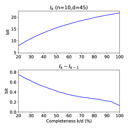
Figure 3: The mutual information between the chain structure and its $k$-step ESPA, $I_{k}$, is concave, suggesting possible benefit of using ESPA. In the simulation, there are $n=10$ items in the chain and thus $d=45$ pairs, $k$ of which are labeled. The values of $I_{k}$’s, as defined by Eq. (3), were obtained through averaging 1000 experiments. We use base-2 logarithm and the unit on y-axis is thus “bit”.

Example 1.

The ranking problem is an important machine learning task and often depends on pairwise comparisons, for which the label set is $\mathcal{L}=\{<,>\}$. For a ranking problem with $n$ items, there are $d=n(n-1)/2$ pairwise comparisons in total. Its structure is a chain following the transitivity constraints, i.e., if $A<B$ and $B<C$, then $A<C$.

A $k$-step ESPA $\mathbf{A}_{k}$ for a chain means that only $k$ (out of $d$) pairs are compared and labeled, resulting in a directed acyclic graph (DAG). In this case, $f(\mathbf{a}_{k})$ is actually counting the number of linear extensions of the DAG, which is known to be #P-complete Brightwell and Winkler (1991), so we do not have a closed-form solution to $I_{k}$. In practice, however, we can use the Kahn’s algorithm and backtracking to simulate with a relatively small $n$, as shown by Fig. 3, where $n=10$ and $I_{k}$ was obtained through averaging 1000 random simulations. $I_{k}$ is concave, as reflected by the downward shape of $I_{k}-I_{k-1}$. Therefore, new annotations are less and less efficient for the chain structure, suggesting the usage of ESPA.

Example 2.

The general assignment problem requires assigning $d$ agents to $d^{\prime}$ tasks such that the agent nodes and the task nodes form a bipartite graph (without loss of generality, assume $d\leq d^{\prime}$). That is, an agent can handle exactly one task, and each task can only be handled by at most one agent. Then from the agents’ point of view, the label set for each of them is $\mathcal{L}=\{1,2,\dots,d^{\prime}\}$, denoting the task assigned to the agent.

A $k$-step ESPA $\mathbf{A}_{k}$ for this problem means that $k$ agents are already assigned with tasks, and $f(\mathbf{a}_{k})$ is to count the valid assignments of the remaining tasks to the remaining $d-k$ agents, to which we have closed-form solutions: $f(\mathbf{a}_{k})=\frac{(d^{\prime}-k)!}{(d^{\prime}-d)!}$, $\forall\mathbf{a}_{k}$. According to Eq. (3), $I_{k}=\log{\frac{d^{\prime}!}{(d^{\prime}-k)!}}$ regardless of $d$ or the distribution of $\mathbf{A}_{k}$, and is concave (Fig. 4 shows an example of it when $d=4,d^{\prime}=10$).

Example 3.

Sequence tagging is an important NLP problem, where the tags of tokens are interdependent. Take chunking as an example. A basic scheme is for each token to choose from three labels, B(egin), I(nside), and O(utside), to represent text chunks in a sentence. That is, $\mathcal{L}=\{B,I,O\}$. Obviously, O cannot be immediately followed by I.

Let $d$ be the number of tokens in a sentence. A $k$-step ESPA $\mathbf{A}_{k}$ for chunking means that $k$ tokens are already labeled by B/I/O, and $f(\mathbf{a}_{k})$ counts the valid BIO sequences that do not violate those existing annotations. Again, as far as we know, there is no closed-form solution to $f(\mathbf{a}_{k})$ and $I_{k}$, but in practice, we can use dynamic programming to obtain $f(\mathbf{a}_{k})$ and then $I_{k}$ using Eq. (3). We set $d=10$ and show $I_{k}-I_{k-1}$ for this task in Fig. 4, where we observe the same effect we see in previous examples: The benefit provided by labeling a new token in the structure attenuates.

Interestingly, based on Fig. 4, we find that the slope of $I_{k}-I_{k-1}$ may be a good measure of the “tightness” or “strength” of a structure. When there is no structure at all, the curve is flat (black). The BIO structure is intuitively simple, and it indeed has the flattest slope among the three structured tasks (purple). When the structure is a chain, the level of uncertainty goes down rapidly with every single annotation (think of standard sorting algorithms); the constraint is intuitively strong and in Fig. 4, it indeed has a steep slope (blue).

Finally, we want to emphasize that the definition of $I_{k}$ in Eq. (3) is in fact backed by information theory. When we do not have prior information about $\mathbf{Y}$, we can assume that $\mathbf{Y}$ follows a uniform distribution over $C(\mathcal{L}^{d})$. Then, $I_{k}$ is essentially the mutual information between structure $\mathbf{Y}$ and annotation $\mathbf{A}_{k}$, $I(\mathbf{Y};\mathbf{A}_{k})$:

$$I(\mathbf{Y};\mathbf{A}_{k}) =H(\mathbf{Y})-H(\mathbf{Y}|\mathbf{A}_{k})$$

$$=\log{|C(\mathcal{L}^{d})|}-E\left[H(\mathbf{Y}|\mathbf{A}_{k}=\mathbf{a}_{k})\right]$$

$$=\log{|C(\mathcal{L}^{d})|}-E\left[\log{f(\mathbf{a}_{k})}\right],$$

where $H(\cdot)$ is the entropy function. This is an important discovery, since it points out a new way to view a structure and its annotations. It may be useful for studying active learning methods for structured tasks, and other annotation phenomena such as noisy annotations. The usage of mutual information also aligns well with the information bottleneck framework Shamir et al. (2010); Shwartz-Ziv and Tishby (2017); Yu and Principe (2018), although a more recent paper challenges the interpretation of information bottleneck Saxe et al. (2018).

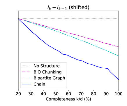
Figure 4: The $I_{k}-I_{k-1}$ curves from several different structures. The curves are shifted to almost the same starting point for better visualization, so the Y-Axis grid is not shown. The curve for “Chain” was obtained via simulations, and the other curves all have closed-form formulations.

3 Learning from Partial Structures

So far, we have been advocating the ESPA strategy to maximize the information we can get from a fixed budget. Since early stopping leads to partial annotations, one missing component before we can benefit from it is an approach to learning from partial structures. In this study, we assume the existence of a relatively small but complete dataset that can provide a good initialization for learning from a partial dataset, which is very similar to semi-supervised learning (SSL). SSL, in its most standard form, studies the combined usage of a labeled set $\mathcal{T}=\{(x_{i},y_{i})\}_{i}$ and an unlabeled set $\mathcal{U}=\{x_{j}\}_{j}$, where the $x$’s are instances and $y$’s are the corresponding labels. SSL gains information about $p(x)$ through $\mathcal{U}$, which may improve the estimation of $p(y|x)$. Specific algorithms range from self-training Scudder (1965); Yarowsky (1995), co-training Blum and Mitchell (1998), generative models Nigam et al. (2000), to transductive SVM Joachims (1999) etc., among which one of the most basic algorithms is Expectation-Maximization (EM) Dempster et al. (1977). By treating them as hidden variables, EM “marginalizes” out the missing labels of $\mathcal{U}$ via expectation (i.e., soft EM) or maximization (i.e., hard EM). For structured ML tasks, soft and hard EMs turn into posterior regularization (PR) Ganchev et al. (2010) and constraint-driven learning (CoDL) Chang et al. (2007), respectively.

Unlike unlabeled data, the partially annotated structures caused by early stopping urge us to gain information not only about $p(x)$, but also from their labeled parts. There have been many existing work along this line Tsuboi et al. (2008); Fernandes and Brefeld (2011); Hovy and Hovy (2012); Lou and Hamprecht (2012), but in this paper, we decide to extend CoDL to cope with partial annotations due to two reasons. First, CoDL, which itself can be viewed as an extension of self-training to structured learning, is a wrapper algorithm having wide applications. Second, as its name suggests, CoDL learns from $\mathcal{U}$ by guidance of constraints, so partial annotations in $\mathcal{U}$ are technically easy to be added as extra equality constraints.

Algorithm 1 describes our Structured Self-learning with Partial ANnotations (SSPAN) algorithm that learns a model $\mathcal{H}$. The same as CoDL, SSPAN is a wrapper algorithm requiring two components: Learn and Inference. Learn attempts to estimate the local decision function for each individual instance regardless of the global constraints, while Inference takes those local decisions and performs a global inference. Lines 1-1 are the procedure of self-training, which iteratively completes the missing annotations in $\mathcal{P}$ and learns from both $\mathcal{T}$ and the completed version of $\mathcal{P}$ (i.e., $\tilde{\mathcal{P}}$). Line 1 requires that the inference follows the structural constraints inherently in the task, turning the algorithm into CoDL; Line 1 enforces those partial annotations in $\mathbf{a}_{i}$, further turning it into SSPAN. In practice, Inference can be realized by the Viterbi or beam search algorithm in sequence tagging, or more generally, by Integer Linear Programming (ILP) Punyakanok et al. (2005); either way, the partial constraints of Line 1 can be easily incorporated.

Input: $\mathcal{T}{}=\{(\mathbf{x}_{i},\mathbf{y}_{i})\}_{i=1}^{N}$, $\mathcal{P}{}=\{(\mathbf{x}_{i},\mathbf{a}_{i})\}_{i=N+1}^{N+M}$

1 Initialize $\mathcal{H}=\textsc{Learn}(\mathcal{T}{})$

2 while convergence criteria not satisfied do

3       $\tilde{\mathcal{P}}=\emptyset$

4       foreach $(\mathbf{x}_{i},\mathbf{a}_{i})\in\mathcal{P}$ do

5             $\hat{\mathbf{y}}_{i}$ = Inference($\mathbf{x}_{i};\mathcal{H}$), such that

6                      $\diamond$  $\hat{\mathbf{y}}_{i}\in C(\mathcal{Y}^{d})$

7                      $\diamond$  $\hat{y}_{i,j}=a_{i,j}$, $\forall a_{i,j}\neq\sqcap$

8             $\tilde{\mathcal{P}}=\tilde{\mathcal{P}}\cup\{(\mathbf{x}_{i},\hat{\mathbf{y}}_{i})\}$

9            

10      $\mathcal{H}=\textsc{Learn}(\mathcal{T}+\tilde{\mathcal{P}})$

11      

12return $\mathcal{H}$

Algorithm 1 Structured Self-learning with Partial Annotations (SSPAN)

4 Experiment

In Sec. 2, we argued from an information theoretic view that ESPA is beneficial for structured tasks if we have a fixed annotation resource. We then proposed SSPAN in Sec. 3 to learn from the resulting partial structures. However, on one hand, there is still a gap between the $I_{k}$ analysis and the actual system performance; on the other hand, whether the benefit can be realized in practice also depends on how effective the algorithm exploits partial annotations. Therefore, it remains to be seen how ESPA works in practice. Here we use three NLP tasks: temporal relation (TempRel) extraction, semantic role classification (SRC), and shallow parsing, analogous to the chain, assignment, and BIO structures, respectively.

For all tasks, we compare the following two schemes in Fig. 5, where we use graph structures for demonstration. Initially, we have a relatively small but complete dataset $\mathcal{T}_{0}$, an unannotated dataset $\mathcal{U}_{0}$, and some budget to annotate $\mathcal{U}_{0}$. The conventional scheme I, also our baseline here, is to annotate each structure completely before randomly picking up the next one. Due to the limited budget, some $\mathcal{U}_{0}$ remain untouched (denoted by $\mathcal{U}$). The proposed scheme II adopts ESPA so that all structures at hand are annotated but only partially. For fair comparisons, we use CoDL to incorporate $\mathcal{U}$ into scheme I as well. Finally, the systems trained on the dataset from I/II via CoDL/SSPAN are evaluated on unseen but complete testset $\mathcal{T}_{test}$. Note that because ESPA is a new annotation scheme, there exists no dataset collected this way. We use existing complete datasets and randomly throw out some annotations to mimic ESPA in the following. Due to the randomness in selecting which structures/instances to keep in scheme I/II, we repeat the whole process multiple times and report the mean $F_{1}$. The budget, defined as the total number of individual instances that can be annotated, ranges from 10% to 100% with a stepsize of 10%, where x% means x% of all instances in $\mathcal{U}_{0}$ can be annotated.

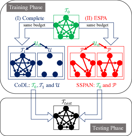
Figure 5: The two annotation schemes we compare in Sec. 4. $\mathcal{T}$, $\mathcal{P}$, and $\mathcal{U}$ denote complete, partial, and empty structures, respectively. Both schemes start with a complete and relatively small dataset and an unannotated dataset (green). (I) Conventional complete annotation scheme (blue). (II) The proposed ESPA scheme (red). Finally, they are tested on an unseen and complete dataset (black).

4.1 Temporal Relation Extraction

Temporal relations (TempRel) are a type of important relations representing the temporal ordering of events described by natural language text. That is to answer questions like which event happens earlier or later in time (see Fig. 1a). Since time is physically one-dimensional, if A is before B and B is also before C, then A must be before C. In practice, the label set for TempRels can be more complex, e.g., with labels such as Simultaneous and Vague, but the structure can still be represented by transitivity constraints (see Table 1 of Ning et al. (2018a)), which can be viewed as an analogy of the chain structure in Example 1.

To avoid missing relations, annotators are required to exhaustively label every pair of events in a document (i.e., the complete annotation scheme), so it is necessary to study ESPA in this context. Here we adopt the MATRES dataset Ning et al. (2018b) for its better inter-annotator agreement and relatively large size.

Specifically, we use 35 documents as $\mathcal{T}_{0}$ (the TimeBank-Dense section, 147 documents as $\mathcal{U}_{0}$ (the TimeBank section minus those documents in $\mathcal{T}_{0}$), and the Platinum section (a benchmark testset of 20 documents with 1K TempRels) as $\mathcal{T}_{test}$. Note that both schemes I and II are mimicked by downsampling the original annotations in MATRES, where the budget is defined as the total number of TempRels that are kept. Following CogCompTime Ning et al. (2018d), we choose the same features and sparse-averaged perceptron algorithm as the Learn component and ILP as Inference for SSPAN.

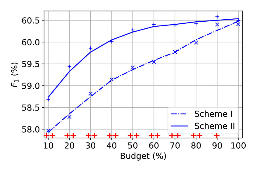
(a) Temporal Relation Extraction

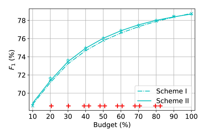
(b) SRC

(c) Shallow Parsing

Figure 6: Comparison of the baseline, complete annotation scheme and the proposed ESPA scheme (See I & II in Fig. 5) under three structured learning tasks (note the scale difference). Each $F_{1}$ value is the average of 50 experiments, and each curve is based on corresponding $F_{1}$ values smoothed by Savitzky-Golay filters. We can see that scheme II is consistently better than scheme I. Per the Wilcoxon rank-sum test, the significance levels at each given budget are shown on the x-axes, where $+$ and $++$ mean $p<5\%$ and $p<1\%$, respectively.

4.2 Semantic Role Classification (SRC)

Semantic role labeling (SRL) is to represent the semantic meanings of language and answer questions like Who did What to Whom and When, Where, How Palmer et al. (2010). Semantic Role Classification (SRC) is a subtask of SRL, which assumes gold predicates and argument chunks and only classifies the semantic role of each argument. We use the Verb SRL dataset provided by the CoNLL-2005 shared task Carreras and Màrquez (2005), where the semantic roles include numbered arguments, e.g., Arg0 and Arg1, and argument modifiers, e.g., location (Am-Loc), temporal (Am-Tmp), and manner (Am-Mnr) (see PropBank Kingsbury and Palmer (2002)). The structural constraints for SRC is that each argument can be assigned to exactly one semantic role, and the same role cannot appear twice for a single verb, so SRC is an assignment problem as in Example 2.

Specifically, we use the Wall Street Journal (WSJ) part of Penn TreeBank III Marcus et al. (1993). We randomly select 700 sentences from the Sec. 24 of WSJ, among which 100 sentences as $\mathcal{T}_{0}$ and 600 sentences as $\mathcal{U}_{0}$. Our $\mathcal{T}_{test}$ is 5700 sentences (about 40K arguments) from Secs. 00, 01, 23. The budget here is defined as the total number of the arguments. We adopt the SRL system in CogCompNLP Khashabi et al. (2018) and uses the sparse averaged perceptron as Learn and ILP as Inference.

4.3 Shallow Parsing

Shallow parsing, also referred as chunking, is a fundamental NLP task to identify constituents in a sentence, such as noun phrases (NP), verb phrases (VP), and adjective phrases (ADJP), which can be viewed as extending the standard BIO structure in Example 3 with different chunk types: B-NP, I-NP, B-VP, I-VP, B-ADJP, I-ADJP, …, O.

We use the chunking dataset provided by the CoNLL-2000 shared task Tjong Kim Sang and Buchholz (2000). Specifically, we use 2K tokens’ annotations as $\mathcal{T}_{0}$, 14K tokens as $\mathcal{U}_{0}$, and the benchmark testset (25K tokens) as $\mathcal{T}_{test}$. The budget here is defined as the total number of tokens’ BIO labels. The algorithm we use here is the chunker provided in CogCompNLP, where the Learn component is the sparse averaged perceptron and the Inference is described in Punyakanok and Roth (2001).

4.4 Results

We compare the $F_{1}$ performances of all three tasks in Fig. 6, averaged from 50 experiments with different randomizations. As the budget increases, the system $F_{1}$ increases for both schemes I and II in all three tasks, which confirms the capability of the proposed SSPAN framework to learn from partial structures. When the budget is 100% (i.e., the entire $\mathcal{U}_{0}$ is annotated), schemes I and II have negligible differences; when the budget is not large enough to cover the entire $\mathcal{U}_{0}$, scheme II is consistently better than I in all tasks, which follows our expectations based on the $I_{k}$ analysis. The strict improvement for all budget ratios indicates that the observation is definitely not by chance.

Figure 7 further compares the improvement from I to II across tasks. When the budget goes down from 100%, the advantage of ESPA is more prominent; but when the budget is too low, the quality of $\tilde{\mathcal{P}}$ degrades and hurts the performance of SSPAN, leading to roughly hill-shaped curves in Fig. 7. We have also conjectured based on Fig. 4 that the structure strength goes up from BIO chunks, to bipartite graphs, and to chains; interestingly, the improvement brought by ESPA is consistent with this order.

Admittedly, the improvement, albeit statistically significant, is small, but it does not diminish the contribution of this paper: Our goal is to remind people that the ESPA scheme (or more generally, partialness) is, at the least, comparable to (or sometimes even better than) complete annotation schemes. Also, the comparison here is in fact unfair to the partial scheme II, because we assume equal cost for both schemes, although it often costs less in a partial scheme as a large problem is decomposed into smaller parts. Therefore, the results shown here implies that the information theoretical benefit of partialness can possibly offset its disadvantages for learning.

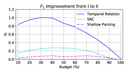
Figure 7: The improvement of $F_{1}$ brought by ESPA for each task in Fig. 6. Note that we conjectured earlier in Fig. 4 that the BIO structure is the weakest among the three, which is consistent with the fact that shallow parsing benefits the least from ESPA.

5 Dicussion and Conclusion

In this paper, we investigate a less studied, yet important question for structured learning: Given a limited annotation budget (either in time or money), which strategy is better, completely annotating each structure until the budget runs out, or annotating more structures at the cost of leaving some of them partially annotated? Neubig and Mori (2010) investigated this issue specifically in annotating word boundaries and pronunciations for Japanese. Instead of annotating full sentences, they proposed to annotate only some words in a sentence (i.e., partially) that can be chosen heuristically (e.g., skip those that we have seen or those low frequency words). Conceptually, Neubig and Mori (2010) is an active learning work, with the understanding that if the order of annotation is deliberately designed, better learning can be achieved. The current paper addresses the problem from a different angle: Even without active learning, can we still answer the question above?

The observation driving our questions is that when annotating a particular structure, the labels of the yet to be labeled variables may already be constrained by previous annotations and carry less information than those in a totally new structure. Therefore, we systematically study the ESPA scheme – stop annotating a given structure before it is completed and continue annotating another new structure.

An important notion is annotation cost. Throughout the paper we have an ideal assumption that the cost is linear in the total number of annotations, but in practice the case can be more complicated. First, the actual cost of each individual annotation may vary across different instances. We try to eliminate this issue by enforcing random selection of annotation instances, rather than allowing the annotators to select arbitrarily by themselves. This strategy may be useful in practice as well, to avoid people only annotating easy cases. Second, even if we only require labeling partial structures, it is likely that the annotator still needs to comprehend the entire structure, incurring additional cost (usually in terms of time). This issue, however, is not addressed in this paper.

Using this definition of cost, we provide a theoretical analysis for ESPA based on the mutual information between target structures and annotation processes. We show that for structures like chains, bipartite graphs, and BIO chunks, the information brought by an extra annotation attenuates as the annotation of the structure is more complete, suggesting to stop early and move to a new structure (although it still remains unclear when it is optimal to stop). This analysis is further supported by experiments on temporal relation extraction, semantic role classification, and shallow parsing, three tasks analogous to the three structures analyzed earlier, respectively. The ratio of the attenuation curve as in Fig. 4 is also shown to be an actionable metric to quantify the strength of a type of structure, which can be useful in various analysis, including judging whether ESPA is worthwhile for a particular task. For example, a more detailed $I_{k}$-based analysis for SRC shows that predicates with more arguments are stronger structures than those with fewer arguments; we have investigated ESPA on those with more than 6 arguments and indeed, observed much larger improvement in SRC. More details on this analysis are put in the appendix.

We think that the findings in this paper are very important. First, as far as we know, we are the first to propose the mutual information analysis that provides a unique view of structured annotation, that of the reduction in the uncertainty of a target of interest $\mathbf{Y}$ by another random variable/process. From this perspective, signals that have non-zero mutual information with $\mathbf{Y}$ can be viewed as “annotations”. These can be partially labeled structures (studied here), partial labels (restricting the possible labels rather than determining a single one as in e.g., Hu et al. (2019), noisy labels (e.g., generated by crowdsourcing or heuristic rules) or, generally, other indirect supervision signals that are correlated with $\mathbf{Y}$. As we proposed, these can be studied within our mutual information framework as well. This paper thus provides a way to analyze the benefit of general incidental supervision signals Roth (2017)) and possibly even provides guidance in selecting good incidental supervision signals.

Second, the findings here open up opportunities for new annotation schemes for structured learning. In the past, partially annotated training data have been either a compromise when completeness is infeasible (e.g., when ranking entries in gigantic databases), or collected freely without human annotators (e.g., based on heuristic rules). If we intentionally ask human annotators for partial annotations, the annotation tasks can be more flexible and potentially, cost even less. This is because annotating complex structures typically require certain expertise, and smaller tasks are often easier Fernandes and Brefeld (2011). It is very likely that some complex annotation tasks require people to read dozens of pages of annotation guidelines, but once decomposed into smaller subtasks, even laymen can handle them. Annotation schemes driven by crowdsourced question-answering, known to provide only partial coverage are successful examples of this idea He et al. (2015); Michael et al. (2017). Therefore, this paper is hopefully interesting to a broad audience.

References

- Ambati et al. (2010) Vamshi Ambati, Stephan Vogel, and Jaime G Carbonell. 2010. Active learning and crowd-sourcing for machine translation. In Proc. of the International Conference on Language Resources and Evaluation (LREC), volume 1, page 2. Citeseer.
- Angluin (1988) Dana Angluin. 1988. Queries and concept learning. Machine Learning, 2(4):319–342.
- Atlas et al. (1990) Les E Atlas, David A Cohn, and Richard E Ladner. 1990. Training connectionist networks with queries and selective sampling. In The Conference on Advances in Neural Information Processing Systems (NIPS), pages 566–573.
- Blum and Mitchell (1998) Avrim Blum and Tom Mitchell. 1998. Combining labeled and unlabeled data with co-training. In Proc. of the Annual ACM Workshop on Computational Learning Theory (COLT).
- Brightwell and Winkler (1991) Graham Brightwell and Peter Winkler. 1991. Counting linear extensions is #p-complete. In Proceedings of the Twenty-third Annual ACM Symposium on Theory of Computing, pages 175–181.
- Carreras and Màrquez (2005) Xavier Carreras and Lluis Màrquez. 2005. Introduction to the CoNLL-2005 shared task: Semantic role labeling. In Proc. of the Annual Conference on Computational Natural Language Learning (CoNLL), pages 152–164.
- Chang et al. (2007) Ming-Wei Chang, Lev Ratinov, and Dan Roth. 2007. Guiding semi-supervision with constraint-driven learning. In Proc. of the Annual Meeting of the Association for Computational Linguistics (ACL), pages 280–287.
- Choi et al. (2018) Jonghyun Choi, Jayant Krishnamurthy, Aniruddha Kembhavi, and Ali Farhadi. 2018. Structured set matching networks for one-shot part labeling. The IEEE Conference on Computer Vision and Pattern Recognition (CVPR).
- Dempster et al. (1977) Arthur P Dempster, Nan M Laird, and Donald B Rubin. 1977. Maximum likelihood from incomplete data via the em algorithm. Journal of the Royal Statistical Society, Series B, 39(1):1–38.
- Fernandes and Brefeld (2011) Eraldo R Fernandes and Ulf Brefeld. 2011. Learning from partially annotated sequences. In Proc. of the Joint European Conference on Machine Learning and Principles and Practice of Knowledge Discovery in Databases (ECML-PKDD).
- Ganchev et al. (2010) Kuzman Ganchev, Jennifer Gillenwater, and Ben Taskar. 2010. Posterior regularization for structured latent variable models. Journal of Machine Learning Research.
- He et al. (2015) Luheng He, Mike Lewis, and Luke Zettlemoyer. 2015. Question-answer driven semantic role labeling: Using natural language to annotate natural language. In Proc. of the Conference on Empirical Methods for Natural Language Processing (EMNLP), pages 643–653.
- Hovy and Hovy (2012) Dirk Hovy and Eduard Hovy. 2012. Exploiting partial annotations with em training. In Proc. of the Annual Meeting of the North American Association of Computational Linguistics (NAACL), pages 31–38.
- Hu et al. (2019) Peiyun Hu, Zack Lipton, Anima Anandkumar, and Deva Ramanan. 2019. Active learning with partial feedback. In Proc. of the International Conference on Learning Representations (ICLR).
- Joachims (1999) Thorsten Joachims. 1999. Transductive inference for text classification using support vector machines. In Proc. of the International Conference on Machine Learning (ICML).
- Khashabi et al. (2018) Daniel Khashabi, Mark Sammons, Ben Zhou, Tom Redman, Christos Christodoulopoulos, Vivek Srikumar, Nicholas Rizzolo, Lev Ratinov, Guanheng Luo, Quang Do, Chen-Tse Tsai, Subhro Roy, Stephen Mayhew, Zhili Feng, John Wieting, Xiaodong Yu, Yangqiu Song, Shashank Gupta, Shyam Upadhyay, Naveen Arivazhagan, Qiang Ning, Shaoshi Ling, and Dan Roth. 2018. Cogcompnlp: Your swiss army knife for nlp. In 11th Language Resources and Evaluation Conference.
- Kingsbury and Palmer (2002) Paul Kingsbury and Martha Palmer. 2002. From Treebank to PropBank. In Proceedings of LREC-2002.
- Laws et al. (2011) Florian Laws, Christian Scheible, and Hinrich Schütze. 2011. Active learning with amazon mechanical turk. In Proc. of the Conference on Empirical Methods for Natural Language Processing (EMNLP), pages 1546–1556.
- Lewis and Gale (1994) David D Lewis and William A Gale. 1994. A sequential algorithm for training text classifiers. In Proc. of International Conference on Research and Development in Information Retrieval, SIGIR, pages 3–12.
- Lou and Hamprecht (2012) Xinghua Lou and Fred A Hamprecht. 2012. Structured learning from partial annotations. In Proc. of the International Conference on Machine Learning (ICML), pages 371–378.
- Marcus et al. (1993) Mitchell P Marcus, Mary Marcinkiewicz, and Beatrice Santorini. 1993. Building a large annotated corpus of English: The Penn Treebank. Computational Linguistics, 19(2):313–330.
- Michael et al. (2017) Julian Michael, Gabriel Stanovsky, Luheng He, Ido Dagan, and Luke Zettlemoyer. 2017. Crowdsourcing question-answer meaning representations. arXiv preprint arXiv:1711.05885.
- Neubig and Mori (2010) Graham Neubig and Shinsuke Mori. 2010. Word-based partial annotation for efficient corpus construction. In Proc. of the International Conference on Language Resources and Evaluation (LREC). Citeseer.
- Nigam et al. (2000) Kamal Nigam, Andrew Kachites Mccallum, Sebastian Thrun, and Tom Mitchell. 2000. Text classification from labeled and unlabeled documents using EM. Machine Learning, 39(2/3):103–134.
- Ning et al. (2018a) Qiang Ning, Zhili Feng, Hao Wu, and Dan Roth. 2018a. Joint reasoning for temporal and causal relations. In Proc. of the Annual Meeting of the Association of Computational Linguistics (ACL), pages 2278–2288.
- Ning et al. (2018b) Qiang Ning, Hao Wu, and Dan Roth. 2018b. A multi-axis annotation scheme for event temporal relations. In Proc. of the Annual Meeting of the Association of Computational Linguistics (ACL), pages 1318–1328.
- Ning et al. (2018c) Qiang Ning, Zhongzhi Yu, Chuchu Fan, and Dan Roth. 2018c. Exploiting partially annotated data for temporal relation extraction. In The Joint Conference on Lexical and Computational Semantics (*Proc. of the Joint Conference on Lexical and Computational Sematics), pages 148–153.
- Ning et al. (2018d) Qiang Ning, Ben Zhou, Zhili Feng, Haoruo Peng, and Dan Roth. 2018d. CogCompTime: A tool for understanding time in natural language. In Proc. of the Conference on Empirical Methods for Natural Language Processing (EMNLP).
- Palmer et al. (2010) Martha Palmer, Daniel Gildea, and Nianwen Xue. 2010. Semantic role labeling, volume 3.
- Punyakanok and Roth (2001) Vasin Punyakanok and Dan Roth. 2001. The use of classifiers in sequential inference. In Proc. of the Conference on Neural Information Processing Systems (NIPS), pages 995–1001.
- Punyakanok et al. (2005) Vasin Punyakanok, Dan Roth, Wen tau Yih, and Dav Zimak. 2005. Learning and inference over constrained output. In Proc. of the International Joint Conference on Artificial Intelligence (IJCAI), pages 1124–1129.
- Roth (2017) Dan Roth. 2017. Incidental supervision: Moving beyond supervised learning. In Proc. of the Conference on Artificial Intelligence (AAAI).
- Roth and Small (2006a) Dan Roth and Kevin Small. 2006a. Active learning with perceptron for structured output. In Proc. of the International Conference on Machine Learning (ICML).
- Roth and Small (2006b) Dan Roth and Kevin Small. 2006b. Margin-based active learning for structured output spaces. In Proc. of the European Conference on Machine Learning (ECML).
- Roth and Small (2008) Dan Roth and Kevin Small. 2008. Active learning for pipeline models. In Proc. of the National Conference on Artificial Intelligence (AAAI).
- Saxe et al. (2018) Andrew M Saxe, Yamini Bansal, Joel Dapello, Madhu Advani, Artemy Kolchinsky, Brendan D Tracey, and David D Cox. 2018. On the information bottleneck theory of deep learning. In Proc. of the International Conference on Learning Representations (ICLR).
- Scudder (1965) H Scudder. 1965. Probability of error of some adaptive pattern-recognition machines. IEEE Transactions on Information Theory, 11(3):363–371.
- Shamir et al. (2010) Ohad Shamir, Sivan Sabato, and Naftali Tishby. 2010. Learning and generalization with the information bottleneck. Theoretical Computer Science, 411(29-30):2696–2711.
- Shwartz-Ziv and Tishby (2017) Ravid Shwartz-Ziv and Naftali Tishby. 2017. Opening the black box of deep neural networks via information. arXiv preprint arXiv:1703.00810.
- Tjong Kim Sang and Buchholz (2000) Erik F. Tjong Kim Sang and Sabine Buchholz. 2000. Introduction to the CoNLL-2000 shared task: Chunking. In Proceedings of the CoNLL-2000 and LLL-2000, pages 127–132.
- Tsuboi et al. (2008) Yuta Tsuboi, Hisashi Kashima, Hiroki Oda, Shinsuke Mori, and Yuji Matsumoto. 2008. Training conditional random fields using incomplete annotations. In Proc. the International Conference on Computational Linguistics (COLING), pages 897–904.
- UzZaman et al. (2013) Naushad UzZaman, Hector Llorens, James Allen, Leon Derczynski, Marc Verhagen, and James Pustejovsky. 2013. SemEval-2013 Task 1: TEMPEVAL-3: Evaluating time expressions, events, and temporal relations. *SEM, 2:1–9.
- Yarowsky (1995) David Yarowsky. 1995. Unsupervised word sense disambiguation rivaling supervied methods. In Proc. of the Annual Meeting of the Association of Computational Linguistics (ACL).
- Yu and Principe (2018) Shujian Yu and Jose C Principe. 2018. Understanding autoencoders with information theoretic concepts. arXiv preprint arXiv:1804.00057.