EMNLP’17
A Structured Learning Approach to Temporal Relation Extraction

Abstract

Identifying temporal relations between events is an essential step towards natural language understanding. However, the temporal relation between two events in a story depends on, and is often dictated by, relations among other events. Consequently, effectively identifying temporal relations between events is a challenging problem even for human annotators. This paper suggests that it is important to take these dependencies into account while learning to identify these relations and proposes a structured learning approach to address this challenge. As a byproduct, this provides a new perspective on handling missing relations, a known issue that hurts existing methods. As we show, the proposed approach results in significant improvements on the two commonly used data sets for this problem.

1 Introduction

Understanding temporal information described in natural language text is a key component of natural language understanding (Mani et al., 2006; Verhagen et al., 2007; Chambers et al., 2007; Bethard and Martin, 2007) and, following a series of TempEval (TE) workshops (Verhagen et al., 2007, 2010; UzZaman et al., 2013), it has drawn increased attention. Time-slot filling (Surdeanu, 2013; Ji et al., 2014), storyline construction (Do et al., 2012; Minard et al., 2015), clinical narratives processing (Jindal and Roth, 2013; Bethard et al., 2016), and temporal question answering (Llorens et al., 2015) are all explicit examples of temporal processing.

The fundamental tasks in temporal processing, as identified in the TE workshops, are 1) time expression (the so-called “timex”) extraction and normalization and 2) temporal relation (also known as TLINKs (Pustejovsky et al., 2003a)) extraction. While the first task has now been well handled by the state-of-the-art systems (HeidelTime (Strötgen and Gertz, 2010), SUTime (Chang and Manning, 2012), IllinoisTime (Zhao et al., 2012), NavyTime (Chambers, 2013), UWTime Lee et al. (2014), etc.) with end-to-end $F_{1}$ scores being around 80%, the second task has long been a challenging one; even the top systems only achieved $F_{1}$ scores of around 35% in the TE workshops.

The goal of the temporal relation task is to generate a directed temporal graph whose nodes represent temporal entities (i.e., events or timexes) and edges represent the TLINKs between them. The task is challenging because it often requires global considerations – considering the entire graph, the TLINK annotation is quadratic in the number of nodes and thus very expensive, and an overwhelming fraction of the temporal relations are missing in human annotation. In this paper, we propose a structured learning approach to temporal relation extraction, where local models are updated based on feedback from global inferences. The structured approach also gives rise to a semi-supervised method, making it possible to take advantage of the readily available unlabeled data. As a byproduct, this approach further provides a new, effective perspective on handling those missing relations.

In the common formulations, temporal relations are categorized into three types: the E-E TLINKs (those between a pair of events), the T-T TLINKs (those between a pair of timexes), and the E-T TLINKs (those between an event and a timex). While the proposed approach can be generally applied to all three types, this paper focuses on the majority type, i.e., the E-E TLINKs. For example, consider the following snippet taken from the training set provided in the TE3 workshop. We want to construct a temporal graph as in Fig. 1 for the events in boldface in Ex1.

1. …tons of earth cascaded down a hillside, ripping two houses from their foundations. No one was hurt, but firefighters ordered the evacuation of nearby homes and said they’ll monitor the shifting ground.…

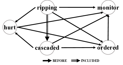
Figure 1: The desired event temporal graph for Ex1. Reverse TLINKs such as hurt is after ripping are omitted for simplicity.

As discussed in existing work (Verhagen, 2004; Bramsen et al., 2006; Mani et al., 2006; Chambers and Jurafsky, 2008), the structure of a temporal graph is constrained by some rather simple rules:

1. Symmetry. For example, if A is before B, then B must be after A.

2. Transitivity. For example, if A is before B and B is before C, then A must be before C.

This particular structure of a temporal graph (especially the transitivity structure) makes its nodes highly interrelated, as can be seen from Fig. 1. It is thus very challenging to identify the TLINKs between them, even for human annotators: The inter-annotator agreement on TLINKs is usually about 50%-60% (Mani et al., 2006). Fig. 2 shows the actual human annotations provided by TE3. Among all the ten possible pairs of nodes, only three TLINKs were annotated. Even if we only look at main events in consecutive sentences and at events in the same sentence, there are still quite a few missing TLINKs, e.g., the one between hurt and cascaded and the one between monitor and ordered.

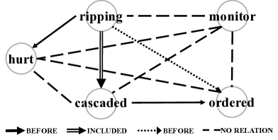
Figure 2: The human-annotation for Ex1 provided in TE3, where many TLINKs are missing due to the annotation difficulty. Solid lines: original human annotations. Dotted lines: TLINKs inferred from solid lines. Dashed lines: missing relations.

Early attempts by Mani et al. (2006); Chambers et al. (2007); Bethard et al. (2007); Verhagen and Pustejovsky (2008) studied local methods – learning models that make pairwise decisions between each pair of events. State-of-the-art local methods, including ClearTK (Bethard, 2013), UTTime (Laokulrat et al., 2013), and NavyTime (Chambers, 2013), use better designed rules or more features such as syntactic tree paths and achieve better results. However, the decisions made by these (local) models are often globally inconsistent (i.e., the symmetry and/or transitivity constraints are not satisfied for the entire temporal graph). Integer linear programming (ILP) methods Roth and Yih (2004) were used in this domain to enforce global consistency by several authors including Bramsen et al. (2006); Chambers and Jurafsky (2008); Do et al. (2012), which formulated TLINK extraction as an ILP and showed that it improves over local methods for densely connected graphs. Since these methods perform inference (“I”) on top of pre-trained local classifiers (“L”), they are often referred to as L+I (Punyakanok et al., 2005). In a state-of-the-art method, CAEVO (Chambers et al., 2014), many hand-crafted rules and machine learned classifiers (called sieves therein) form a pipeline. The global consistency is enforced by inferring all possible relations before passing the graph to the next sieve. This best-first architecture is conceptually similar to L+I but the inference is greedy, similar to Mani et al. (2007); Verhagen and Pustejovsky (2008).

Although L+I methods impose global constraints in the inference phase, this paper argues that global considerations are necessary in the learning phase as well (i.e., structured learning). In parallel to the work presented here, Leeuwenberg and Moens (2017) also proposed a structured learning approach to extracting the temporal relations. Their work focuses on a domain-specific dataset from Clinical TempEval (Bethard et al., 2016), so their work does not need to address some of the difficulties of the general problem that our work addresses. More importantly, they compared structured learning to local baselines, while we find that the comparison between structured learning and L+I is more interesting and important for understanding the effect of global considerations in the learning phase. In difference from existing methods, we also discuss how to effectively use unlabeled data and how to handle the overwhelming fraction of missing relations in a principled way. Our solution targets on these issues and, as we show, achieves significant improvements on two commonly used evaluation sets.

The rest of this paper is organized as follows. Section 2 clarifies the temporal relation types and the evaluation metric of a temporal graph used in this paper, Section 3 explains the structured learning approach in detail, and Section 4 discusses the practical issue of missing relations. We provide experiments and discussion in Section 5 and conclusion in Section 6.

2 Background

2.1 Temporal Relation Types

Existing corpora for temporal processing often follows the interval representation of events proposed in Allen (1984), and makes use of 13 relation types in total. In many systems, vague or none is also included as another relation type when a TLINK is not clear or missing. However, current systems usually use a reduced set of relation types, mainly due to the following reasons.

1. The non-uniform distribution of all the relation types makes it difficult to separate low-frequency ones from the others (see Table 1 in Mani et al. (2006)). For example, relations such as immediately_before or immediately_after barely exist in a corpus compared to before and after.

2. Due to the ambiguity in natural language, determining relations like before and immediately_before can be a difficult task itself (Chambers et al., 2014).

In this work, we follow the reduced set of temporal relation types used in CAEVO (Chambers et al., 2014): before, after, includes, is_included, equal, and vague.

2.2 Quality of A Temporal Graph

The most recent evaluation metric in TE3, i.e., the temporal awareness (UzZaman and Allen, 2011), is adopted in this work. Specifically, let $G_{sys}$ and $G_{true}$ be two temporal graphs from the system prediction and the ground truth, respectively. The precision and recall of temporal awareness are defined as follows.

$$P=\frac{|G_{sys}^{-}\cap G_{true}^{+}|}{|G_{sys}^{-}|},~{}R=\frac{|G_{true}^{-}\cap G_{sys}^{+}|}{|G_{true}^{-}|}$$

where $G^{+}$ is the closure of graph $G$, $G^{-}$ is the reduction of $G$, “$\cap$” is the intersection between TLINKs in two graphs, and $\lvert G\rvert$ is the number of TLINKs in $G$. The temporal awareness metric better captures how “useful” a temporal graph is. For example, if system 1 produces ripping is before hurt and hurt is before monitor, and system 2 adds ripping is before monitor on top of system 1. Since system 2 is simply a transitive closure of system 1, they would have the same evaluation scores. Note that vague relations are usually considered as non-existing TLINKs and are not counted during evaluation.

3 A Structured Training Approach

As shown in Fig. 1, the learning problem in temporal relation extraction is global in nature. Even the top local method in TE3, UTTime (Laokulrat et al., 2013), only achieved $F_{1}$=56.5 when presented with a pair of temporal entities (Task C–relation only (UzZaman et al., 2013)). Since the success of an L+I method strongly relies on the quality of the local classifiers, a poor local classifier is obviously a roadblock for L+I methods. Following the insights from Punyakanok et al. (2005), we propose to use a structured learning approach (also called “Inference Based Training” (IBT)).

Unlike the current L+I approach, where local classifiers are trained independently beforehand without knowledge of the predictions on neighboring pairs, we train local classifiers with feedback that accounts for other relations, by performing global inference in each round of the learning process. In order to introduce the structured learning algorithm, we first explain its most important component, the global inference step.

3.1 Inference

In a document with $n$ pairs of events, let $\phi_{i}\in\mathcal{X}\subseteq{}^{d}$ be the extracted $d$-dimensional feature and $y_{i}\in\mathcal{Y}$ be the temporal relation for the $i$-th pair of events, $i=1,2,\dots,n$, where $\mathcal{Y}=\{r_{j}\}_{j=1}^{6}$ is the label set for the six temporal relations we use. Moreover, let $\mathbf{x}=\{\phi_{1},\dots,\phi_{n}\}\in\mathcal{X}^{n}$ and $\mathbf{y}=\{y_{1},\dots,y_{n}\}\in\mathcal{Y}^{n}$ be more compact representations of all the features and labels in this document. Given the weight vector $\mathbf{w}_{r}$ of a linear classifier trained for relation $r\in\mathcal{Y}$ (i.e., using the one-vs-all scheme), the global inference step is to solve the following constrained optimization problem:

$$\hat{\mathbf{y}}=\textrm{arg}\max_{\mathbf{y}\in\mathcal{C}(\mathcal{Y}^{n})}{f(\mathbf{x},\mathbf{y})},$$ (1)

where $\mathcal{C}(\mathcal{Y}^{n})\subseteq\mathcal{Y}^{n}$ constrains the temporal graph to be symmetrically and transitively consistent, and $f(\mathbf{x},\mathbf{y})$ is the scoring function:

$$f(\mathbf{x},\mathbf{y})=\sum_{i=1}^{n}{f_{y_{i}}(\phi_{i})}=\sum_{i=1}^{n}{\frac{e^{\mathbf{w}_{y_{i}}^{T}\phi_{i}}}{\sum_{r\in\mathcal{Y}}{e^{\mathbf{w}_{r}^{T}\phi_{i}}}}}.$$

Specifically, $f_{y_{i}}(\phi_{i})$ is the probability of the $i$-th event pair having relation $y_{i}$. $f(x,y)$ is simply the sum of these probabilities over all the event pairs in a document, which we think of as the confidence of assigning $\mathbf{y}=\{y_{1},...,y_{n}\}$ to this document and therefore, it needs to be maximized in Eq. (1).

Note that when $\mathcal{C}(\mathcal{Y}^{n})=\mathcal{Y}^{n}$, Eq. (1) can be solved for each $\hat{y}_{i}$ independently, which is what the so-called local methods do, but the resulting $\hat{\mathbf{y}}$ may not satisfy global consistency in this way. When $\mathcal{C}(\mathcal{Y}^{n})\neq\mathcal{Y}^{n}$, Eq. (1) cannot be decoupled for each $\hat{y}_{i}$ and is usually formulated as an ILP problem (Roth and Yih, 2004; Chambers and Jurafsky, 2008; Do et al., 2012). Specifically, let $\mathcal{I}_{r}(ij)\in\{0,1\}$ be the indicator function of relation $r$ for event $i$ and event $j$ and $f_{r}(ij)\in[0,1]$ be the corresponding soft-max score. Then the ILP objective for global inference is formulated as follows.

$$\hat{\mathcal{I}}=\textrm{arg}\underset{\mathcal{I}}{\textrm{max}}\sum_{ij\in\mathcal{E}}\sum_{r\in\mathcal{Y}}f_{r}(ij)\mathcal{I}_{r}(ij)$$ (2)

$$\textrm{s.t.}\quad\underset{\textrm{(uniqueness)}}{\Sigma_{r}{\mathcal{I}_{r}(ij)}=1},~{}\underset{\textrm{(symmetry)}}{\mathcal{I}_{r}(ij)=\mathcal{I}_{\bar{r}}(ji),}$$

$$\underset{\textrm{(transitivity)}}{\mathcal{I}_{r_{1}}(ij)+\mathcal{I}_{r_{2}}(jk)-\Sigma_{m=1}^{N}\mathcal{I}_{r_{3}^{m}}(ik)\leq 1,}$$

for all distinct events $i$, $j$, and $k$, where $\mathcal{E}=\{ij~{}|~{}\textrm{sentence dist$(i,j)$$\leq 1$}\}$, $\bar{r}$ is the reverse of $r$, and $N$ is the number of possible relations for $r_{3}$ when $r_{1}$ and $r_{2}$ are true.

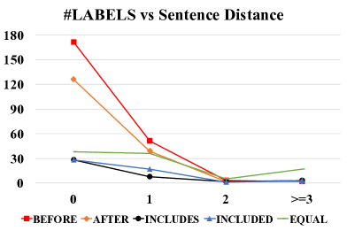
Figure 3: #TLINKs vs sentence distance on the TE3 Platinum dataset. The tail of equal is due to event coreference and beyond our focus.

Our formulation in Eq. (2) is different from previous work (Chambers and Jurafsky, 2008; Do et al., 2012) in two aspects: 1) We restrict our event pairs $ij$ to a smaller set $\mathcal{E}=\{ij~{}|~{}\textrm{sentence dist$(i,j)$$\leq 1$}\}$ where pairs that are more than one sentence away are deleted for computational efficiency and (usually) for better performance. In fact, to make better use of global constraints, we should have allowed more event pairs in Eq. (2). However, $f_{r}(ij)$ is usually more reliable when $i$ and $j$ are closer in text. Many participating systems in TE3 (UzZaman et al., 2013) have used this pre-filtering strategy to balance the trade-off between confidence in $f_{r}(ij)$ and global constraints. We observe that the strategy fits very well to the existing datasets: As shown in Fig. 3, annotated TLINKs barely exist if two events are two sentences away. 2) Previously, transitivity constraints were formulated as $\mathcal{I}_{r_{1}}(ij)+\mathcal{I}_{r_{2}}(jk)-\mathcal{I}_{r_{3}}(ik)\leq 1$, which is a special case when $N=1$ and can be understood as “$r_{1}$ and $r_{2}$ determine a single $r_{3}$”. However, it was overlooked that, although some $r_{1}$ and $r_{2}$ cannot uniquely determine $r_{3}$, they can still constrain the set of labels $r_{3}$ can take. For example, as shown in Fig. 4, when $r_{1}$=before and $r_{2}$=is_included, $r_{3}$ is not determined but we know that $r_{3}\in\{$before, is_included$\}$. This information can be easily exploited by allowing $N>1$.

Figure 4: When A is before B and B is_included in C, A can either be before C₁ or is_included in C₂. We propose to incorporate this via the transitivity constraints for Eq. (2).

With these two differences, the optimization problem (2) can still be efficiently solved using off-the-shelf ILP packages such as GUROBI (Gurobi Optimization, Inc., 2012).

3.2 Learning

With the inference solver defined above, we propose to use the structured perceptron (Collins, 2002) as a representative for the inference based training (IBT) algorithm to learn those weight vectors $\mathbf{w}_{r}$. Specifically, let $\mathcal{L}=\{\mathbf{x}_{k},\mathbf{y}_{k}\}_{k=1}^{K}$ be the labeled training set of $K$ instances (usually documents). The structured perceptron training algorithm for this problem is shown in Algorithm 1. The Illinois-SL package (Chang et al., 2010) was used in our experiments for its structured perceptron component. In terms of the features used in this work, we adopt the same set of features designed for E-E TLINKs in Sec. 3.1 of Do et al. (2012).

In Algorithm 1, Line 1 is the inference step as in Eq. (1) or (2), which is augmented with a closure operation on $\hat{\mathbf{y}}$ in the following line. In the case in which there is only one pair of events in each instance (thus no structure to take advantage of), Algorithm 1 reduces to the conventional perceptron algorithm and Line 1 simply chooses the top scoring label. With a structured instance instead, Line 1 becomes slower to solve, but it can provide valuable information so that the perceptron learner is able to look further at other labels rather than an isolated pair. For example in Ex1 and Fig. 1, the fact that (ripping,ordered)=before is established through two other relations: 1) ripping is an adverbial participle and thus included in cascaded and 2) cascaded is before ordered. If (ripping,ordered)=before is presented to a local learning algorithm without knowing its predictions on (ripping,cascaded) and (cascaded,ordered), then the model either cannot support it or overfits it. In IBT, however, if the classifier was correct in deciding (ripping,cascaded) and (cascaded,ordered), then (ripping,ordered) would be correct automatically and would not contribute to updating the classifier.

Input: Training set $\mathcal{L}=\{\mathbf{x}_{k},\mathbf{y}_{k}\}_{k=1}^{K}$, learning rate $\lambda$

1 Perform graph closure on each $\mathbf{y}_{k}$

2 Initialize $\mathbf{w}_{r}=\mathbf{0}$, $\forall r\in\mathcal{Y}$

3 while convergence criteria not satisfied do

4       Shuffle the examples in $\mathcal{L}$

5       foreach $(\mathbf{x},\mathbf{y})\in\mathcal{L}$ do

6             $\hat{\mathbf{y}}=\textrm{arg}\max_{\mathbf{y}\in\mathcal{C}}{f(\mathbf{x},\mathbf{y})}$

7             Perform graph closure on $\hat{\mathbf{y}}$

8             if $\hat{\mathbf{y}}\neq\mathbf{y}$ then

9                   $\mathbf{w}_{r}=\mathbf{w}_{r}+\lambda(\sum_{i:\mathbf{y}_{i}=r}{\phi_{i}}-$ $\sum_{i:\hat{\mathbf{y}}_{i}=r}{\phi_{i}})$, $\forall r\in\mathcal{Y}$

10                  

11            

12      

13return $\{\mathbf{w}_{r}\}_{r\in\mathcal{Y}}$

Algorithm 1 Structured perceptron algorithm for temporal relations

3.3 Semi-supervised Structured Learning

The scarcity of training data and the difficulty in annotation have long been a bottleneck for temporal processing systems. Given the inherent global constraints in temporal graphs, we propose to perform semi-supervised structured learning using the constraint-driven learning (CoDL) algorithm (Chang et al., 2007, 2012), as shown in Algorithm 2, where the function “Learn” in Lines 2 and 2 represents any standard learning algorithm (e.g., perceptron, SVM, or even structured perceptron; here we used the averaged perceptron Freund and Schapire (1998)) and subscript “$r$” means selecting the learned weight vector for relation $r\in\mathcal{Y}$. CoDL improves the model learned from a small amount of labeled data by repeatedly generating feedback through labeling unlabeled examples, which is in fact a semi-supervised version of IBT. Experiments show that this scheme is indeed helpful in this problem.

Input: Labeled set $\mathcal{L}$, unlabeled set $\mathcal{U}$, weighting coefficient $\gamma$

1 Perform closure on each graph in $\mathcal{L}$

2 Initialize $\mathbf{w}_{r}=\textrm{Learn}(\mathcal{L})_{r},\forall~{}r\in\mathcal{Y}$

3 while convergence criteria not satisfied do

4       $\mathcal{T}=\emptyset$

5       foreach $\mathbf{x}\in\mathcal{U}$ do

6             $\hat{\mathbf{y}}=\textrm{arg}\max_{\mathbf{y}\in\mathcal{C}}{f(\mathbf{x},\mathbf{y})}$

7             Perform graph closure on $\hat{\mathbf{y}}$

8             $\mathcal{T}=\mathcal{T}\cup\{(\mathbf{x},\hat{\mathbf{y}})\}$

9            

10      $\mathbf{w}_{r}=\gamma\mathbf{w}_{r}+(1-\gamma)\textrm{Learn}(\mathcal{T})_{r},\forall~{}r\in\mathcal{Y}$

11      

12return $\{\mathbf{w}_{r}\}_{r\in\mathcal{Y}}$

Algorithm 2 Constraint-driven learning algorithm

4 Missing Annotations

Since even human annotators find it difficult to annotate temporal graphs, many of the TLINKs are left unspecified by annotators (compare Fig. 2 to Fig. 1). While some of these missing TLINKs can be inferred from existing ones, the vast majority still remain unknown as shown in Table 1. Despite the existence of denser annotation schemes (e.g., Cassidy et al. (2014)), the TLINK annotation task is quadratic in the number of nodes, and it is practically infeasible to annotate complete graphs. Therefore, the problem of identifying these unknown relations in training and test is a major issue that dramatically hurts existing methods.

Table 1: Categories of E-E TLINKs in the TE3 Platinum dataset. Among all pairs of events, 98.2% of them are left unspecified by the annotators. Graph closure can automatically add 8.7%, but most of the event pairs are still unknown.

Type		#TLINK	%
Annotated		582	1.8
Missing	Inferred	2840	8.7
	Unknown	29240	89.5
Total		32662	100

We could simply use these unknown pairs (or some filtered version of them) to design rules or train classifiers to identify whether a TLINK is vague or not. However, we propose to exclude both the unknown pairs and the vague classifier from the training process – by changing the structured loss function to ignore the inference feedback on vague TLINKs (see Line 1 in Algorithm 1 and Line 2 in Algorithm 2). The reasons are discussed below.

First, it is believed that a lot of the unknown pairs are not really vague but rather pairs that the annotators failed to look at (Bethard et al., 2007; Cassidy et al., 2014; Chambers et al., 2014). For example, (cascaded, monitor) should be annotated as before but is missing in Fig. 2. It is hard to exclude this noise in the data during training. Second, compared to the overwhelmingly large number of unknown TLINKs (89.5% as shown in Table 1), the scarcity of non-vague TLINKs makes it hard to learn a good vague classifier. Third, vague is fundamentally different from the other relation types. For example, if a before TLINK can be established given a sentence, then it always holds as before regardless of other events around it, but if a TLINK is vague given a sentence, it may still change to other types afterwards if a connection can later be established through other nodes from the context. This distinction emphasizes that vague is a consequence of lack of background/contextual information, rather than a concrete relation type to be trained on. Fourth, without the vague classifier, the predicted temporal graph tends to become more densely connected, thus the global transitivity constraints can be more effective in correcting local mistakes (Chambers and Jurafsky, 2008).

However, excluding the local classifier for vague TLINKs would undesirably assign non-vague TLINKs to every pair of events. To handle this, we take a closer look at the vague TLINKs. We note that a vague TLINK could arise in two situations if the annotators did not fail to look at it. One is that an annotator looks at this pair of events and decides that multiple relations can exist, and the other one is that two annotators disagree on the relation (similar arguments were also made in Cassidy et al. (2014)). In both situations, the annotators first try to assign all possible relations to a TLINK, and then change the relation to vague if more than one can be assigned. This human annotation process for vague is different from many existing methods, which either identify the existence of a TLINK first (using rules or machine-learned classifiers) and then classify, or directly include vague as a classification label along with other non-vague relations.

In this work, however, we propose to mimic this mental process by a post-filtering method. Specifically, we take each TLINK produced by ILP and determine whether it is vague using its relative entropy (the Kullback-Leibler divergence) to the uniform distribution. Let $\{r_{m}\}_{m=1}^{M}$ be the set of relations that the $i$-th pair of events can take, we filter the $i$-th TLINK given by ILP by:

$$\delta_{i}=\sum_{m=1}^{M}{f_{r_{m}}(\phi_{i})\log{\left(Mf_{r_{m}}(\phi_{i})\right)}},$$

where $f_{r_{m}}(\phi_{i})$ is the soft-max score of $r_{m}$, obtained by the local classifier for $r_{m}$. We then compare $\delta_{i}$ to a fixed threshold $\tau$ to determine the vagueness of this TLINK; we accept its originally predicted label if $\delta_{i}>\tau$, or change it to vague otherwise. Using relative entropy here is intuitively appealing and empirically useful as shown in the experiments section; better metrics are of course yet to be designed.

5 Experiments

5.1 Datasets

The TempEval3 (TE3) workshop (UzZaman et al., 2013) provided the TimeBank (TB) (Pustejovsky et al., 2003b), AQUAINT (AQ) (Graff, 2002), Silver (TE3-SV), and Platinum (TE3-PT) datasets, where TB and AQ are usually for training, and TE3-PT is usually for testing. The TE3-SV dataset is a much larger, machine-annotated and automatically-merged dataset based on multiple systems, with the intention to see if these “silver” standard data can help when included in training (although almost all participating systems saw performance drop with TE3-SV included in training).

Two popular augmentations on TB are the Verb-Clause temporal relation dataset (VC) and TimebankDense dataset (TD). The VC dataset has specially annotated event pairs that follow the so-called Verb-Clause structure (Bethard et al., 2007), which is usually beneficial to be included in training (UzZaman et al., 2013). The TD dataset contains 36 documents from TB which were re-annotated using the dense event ordering framework proposed in Cassidy et al. (2014). The experiments included in this paper will involve the TE3 datasets as well as these augmentations. Therefore, some statistics on them are shown in Table 2 for the readers’ information.

Table 2: Facts about the datasets used in this paper. The TD dataset is split into train, dev, and test in the same way as in Chambers et al. (2014). Note that the column of TLINKs only counts the non-vague TLINKs, from which we can see that the TD dataset has a much higher ratio of #TLINKs to #Events. The TLINK annotations in TE3-SV is not used in this paper and its number is thus not shown.

Dataset	Doc	Event	TLINK	Note
TB+AQ	256	12K	12K	Training
VC	132	1.6K	0.9K	Training
TD	36	1.6K	5.7K	Training
TD-Train	22	1K	3.8K	Training
TD-Dev	5	0.2K	0.6K	Dev
TD-Test	9	0.4K	1.3K	Eval
TE3-PT	20	0.7K	0.9K	Eval
TE3-SV	2.5K	81K	-	Unlabeled

5.2 Baseline Methods

In addition to the state-of-the-art systems, another two baseline methods were also implemented for a better understanding of the proposed ones. The first is the regularized averaged perceptron (AP) (Freund and Schapire, 1998) implemented in the LBJava package (Rizzolo and Roth, 2010) and is a local method. On top of the first baseline, we performed global inference in Eq.(2), referred to as the L+I baseline (AP+ILP). Both of them used the same feature set (i.e., as designed in Do et al. (2012)) as in the proposed structured perceptron (SP) and CoDL for fair comparisons. To clarify, SP and CoDL are training algorithms and their immediate outputs are the weight vectors $\{\mathbf{w}_{r}\}_{r\in\mathcal{Y}}$ for local classifiers. An ILP inference was performed on top of them to yield the final output, and we refer to it as “S+I” (i.e., structured learning+inference) methods.

Table 3: Temporal awareness scores on TE3-PT given gold event pairs. Systems that are significantly better (per McNemar’s test with $p<0.0005$) than the previous rows are underlined. The last column shows the relative improvement in F1 score over AP-1, which identifies the source of improvement: 5.2% from additional training data, 9.3% (14.5%-5.2%) from constraints, and 10.4% from structured learning.

Method	P	R	F1	%
UTTime	55.6	57.4	56.5	+5.0
AP-1	56.3	51.5	53.8	0
AP-2	58.0	55.3	56.6	+5.2
AP+ILP	62.2	61.1	61.6	+14.5
SP+ILP	69.1	65.5	67.2	+24.9

5.3 Results and Discussion

5.3.1 TE3 Task C - Relation Only

To show the benefit of using structured learning, we first tested one scenario where the gold pairs of events that have a non-vague TLINK were known priori. This setup was a standard task presented in TE3, so that the difficulty of detecting vague TLINKs was ruled out. This setup also helps circumvent the issue that TE3 penalizes systems which assign extra labels that do not exist in the annotated graph, while these extra labels may be actually correct because the annotation itself might be incomplete. UTTime (Laokulrat et al., 2013) was the top system in this task in TE3. Since UTTime is not available to us, and its performance was reported in TE3 in terms of both E-E and E-T TLINKs together, we locally trained an E-T classifier based on Do et al. (2012) and included its prediction only for fair comparison.

Table 4: Temporal awareness scores given gold events but with no gold pairs, which show that the proposed S+I methods outperformed state-of-the-art systems in various settings. The fourth column indicates the annotation sources used, with additional unlabeled dataset in the parentheses. The “Filters” column shows if the pre-filtering method (Sec. 3.1) or the proposed post-filtering method (Sec. 4) were used. The last column is the relative improvement in $F_{1}$ score compared to baseline systems on line 1, 7, and 11, respectively. Systems that are significantly better than the “*”-ed systems are underlined (per McNemar’s test with $p<0.0005$).

No.	System	Method	Anno. (Unlabeled)	Testset	Filters	P	R	F1	%
1	ClearTK	Local	TB, AQ, VC, TD	TE3-PT	pre	37.2	33.1	35.1	0
2	AP*	Local	TB, AQ, VC, TD	TE3-PT	pre	35.3	37.1	36.1	+2.8
3	AP+ILP	L+I	TB, AQ, VC, TD	TE3-PT	pre	35.7	35.0	35.3	+0.6
4	SP+ILP	S+I	TB, AQ, VC, TD	TE3-PT	pre	32.4	45.2	37.7	+7.4
5	SP+ILP	S+I	TB, AQ, VC, TD	TE3-PT	pre+post	33.1	49.2	39.6	+12.8
6	CoDL+ILP	S+I	TB, AQ, VC, TD (TE3-SV)	TE3-PT	pre+post	35.5	46.5	40.3	+14.8
7	ClearTK*	Local	TB, VC	TE3-PT	pre	35.9	38.2	37.0	0
8	SP+ILP	S+I	TB, VC	TE3-PT	pre+post	30.7	47.1	37.2	+0.5
9	CoDL+ILP	S+I	TB, VC (TE3-SV)	TE3-PT	pre+post	33.9	45.9	39.0	+5.4
10	ClearTK	Local	TD-Train	TD-Test	pre	46.04	20.90	28.74	-
11	CAEVO*	L+I	TD-Train	TD-Test	pre	54.17	39.49	45.68	0
12	SP+ILP	S+I	TD-Train	TD-Test	pre+post	45.34	48.68	46.95	+3.0
13	CoDL+ILP	S+I	TD-Train (TE3-SV)	TD-Test	pre+post	45.57	51.89	48.53	+6.3

UTTime is a local method and was trained on TB+AQ and tested on TE3-PT. We used the same datasets for our local baseline and its performance is shown in Table 3 under the name “AP-1”. Note that the reported numbers below are the temporal awareness scores obtained from the official evaluation script provided in TE3. We can see that UTTime is about 3% better than AP-1 in the absolute value of $F_{1}$, which is expected since UTTime included more advanced features derived from syntactic parse trees. By adding the VC and TD datasets into the training set, we retrained our local baseline and achieved comparable performance to UTTime (“AP-2” in Table 3). On top of AP-2, a global inference step enforcing symmetry and transitivity constraints (“AP+ILP”) can further improve the $F_{1}$ score by 9.3%, which is consistent with previous observations (Chambers and Jurafsky, 2008; Do et al., 2012). SP+ILP further improved the performance in precision, recall, and $F_{1}$ significantly (per the McNemar’s test (Everitt, 1992; Dietterich, 1998) with $p<$0.0005), reaching an $F_{1}$ score of 67.2%. This meets our expectation that structured learning can be better when the local problem is difficult (Punyakanok et al., 2005).

5.3.2 TE3 Task C

In the first scenario, we knew in advance which TLINKs existed or not, so the “pre-filtering” (i.e., ignoring distant pairs as mentioned in Sec. 3.1 and “post-filtering” methods were not used when generating the results in Table 3. We then tested a more practical scenario, where we only knew the events, but did not know which ones are related. This setup was Task C in TE3 and the top system was ClearTK (Bethard, 2013). Again, for fair comparison, we simply added the E-T TLINKs predicted by ClearTK. Moreover, 10% of the training data was held out for development. Corresponding results on the TE3-PT testset are shown in Table 4.

From lines 2-4, all systems see significant drops in performance if compared with the same entries in Table 3. It confirms our assertion that how to handle vague TLINKs is a major issue for this temporal relation extraction problem. The improvement of SP+ILP (line 4) over AP (line 2) was small and AP+ILP (line 3) was even worse than AP, which necessitates the use of a better approach towards vague TLINKs. By applying the post-filtering method proposed in Sec. 4, we were able to achieve better performances using SP+ILP (line 5), which shows the effectiveness of this strategy. Finally, by setting $\mathcal{U}$ in Algorithm 2 to be the TE3-SV dataset, CoDL+ILP (line 6) achieved the best $F_{1}$ score with a relative improvement over ClearTK being 14.8%. Note that when using TE3-SV in this paper, we did not use its annotations on TLINKs because of its well-known large noise (UzZaman et al., 2013).

In UzZaman et al. (2013), we notice that the best performance of ClearTK was achieved when trained on TB+VC (line 7 is higher than its reported values in TE3 because of later changes in ClearTK), so we retrained the proposed systems on the same training set and results are shown on lines 8-9. In this case, the improvement of S+I over Local was small, which may be due to the lack of training data. Note that line 8 was still significantly different to line 7 per the McNemar’s test, although there was only 0.2% absolute difference in $F_{1}$, which can be explained from their large differences in precision and recall.

5.3.3 Comparison with CAEVO

The proposed structured learning approach was further compared to a recent system, a CAscading EVent Ordering architecture (CAEVO) proposed in Chambers et al. (2014) (lines 10-13). We used the same training set and test set as CAEVO in the S+I systems. Again, we added the E-T TLINKs predicted by CAEVO to both S+I systems. In Chambers et al. (2014), CAEVO was reported on the straightforward evaluation metric including the vague TLINKs, but the temporal awareness scores were used here, which explains the difference between line 11 in Table 4 and what was reported in Chambers et al. (2014).

ClearTK was reported to be outperformed by CAEVO on TD-Test (Chambers et al., 2014), but we observe that ClearTK on line 10 was much worse even than itself on line 7 (trained on TB+VC) and on line 1 (trained on TB+AQ+VC+TD) due to the annotation scheme difference between TD and TB/AQ/VC. ClearTK was designed mainly for TE3, aiming for high precision, which is reflected by its high precision on line 10, but it does not have enough flexibility to cope with two very different annotation schemes. Therefore, we have chosen CAEVO as the baseline system to evaluate the significance of the proposed ones. On the TD-Test dataset, all systems other than ClearTK had better $F_{1}$ scores compared to their performances on TE3-PT. This notable difference (i.e., 48.53 vs 40.3) indicates the better quality of the dense annotation scheme that was used to create TD (Cassidy et al., 2014). SP+ILP outperformed CAEVO and if additional unlabeled dataset TE3-SV was used, CoDL+ILP achieved the best score with a relative improvement in $F_{1}$ score being 6.3%.

We notice that the proposed systems often have higher recall than precision, and that this is less an issue on a densely annotated testset (TD-Test), so their low precision on TE3-PT possibly came from the missing annotations on TE3-PT. It is still under investigation how to control precision and recall in real applications.

6 Conclusion

We develop a structured learning approach to identifying temporal relations in natural language text and show that it captures the global nature of this problem better than state-of-the-art systems do. A new perspective towards vague relations is also proved to gain from fully taking advantage of the structured approach. In addition, the global nature of this problem gives rise to a better way of making use of the readily available unlabeled data, which further improves the proposed method. The improved performance on both TE3-PT and TD-Test, two differently annotated datasets, clearly shows the advantage of the proposed method over existing methods. We plan to build on the notable improvements shown here and expand this study to deal with additional temporal reasoning problems in natural language text.

References

- Allen (1983) James F Allen. 1983. Maintaining knowledge about temporal intervals. Communications of the ACM 26(11):832–843.
- Allen (1984) James F Allen. 1984. Towards a general theory of action and time. Artificial intelligence 23(2):123–154.
- Bethard (2013) Steven Bethard. 2013. ClearTK-TimeML: A minimalist approach to TempEval 2013. In Second Joint Conference on Lexical and Computational Semantics (* SEM). volume 2, pages 10–14.
- Bethard and Martin (2007) Steven Bethard and James H Martin. 2007. CU-TMP: Temporal relation classification using syntactic and semantic features. In Proceedings of the 4th International Workshop on Semantic Evaluations. Association for Computational Linguistics, pages 129–132.
- Bethard et al. (2007) Steven Bethard, James H Martin, and Sara Klingenstein. 2007. Timelines from text: Identification of syntactic temporal relations. In Semantic Computing, 2007. ICSC 2007. International Conference on. IEEE, pages 11–18.
- Bethard et al. (2016) Steven Bethard, Guergana Savova, Wei-Te Chen, Leon Derczynski, James Pustejovsky, and Marc Verhagen. 2016. SemEval-2016 Task 12: Clinical TempEval. Proceedings of SemEval pages 1052–1062.
- Bramsen et al. (2006) P. Bramsen, P. Deshpande, Y. K. Lee, and R. Barzilay. 2006. Inducing temporal graphs. In Proceedings of the Conference on Empirical Methods for Natural Language Processing (EMNLP). Association for Computational Linguistics, Sydney, Australia, pages 189–198.
- Cassidy et al. (2014) Taylor Cassidy, Bill McDowell, Nathanel Chambers, and Steven Bethard. 2014. An annotation framework for dense event ordering. Technical report, DTIC Document.
- Chambers and Jurafsky (2008) N. Chambers and D. Jurafsky. 2008. Jointly combining implicit constraints improves temporal ordering. In Proceedings of the Conference on Empirical Methods for Natural Language Processing (EMNLP).
- Chambers (2013) Nathanael Chambers. 2013. NavyTime: Event and time ordering from raw text. Technical report, DTIC Document.
- Chambers et al. (2014) Nathanael Chambers, Taylor Cassidy, Bill McDowell, and Steven Bethard. 2014. Dense event ordering with a multi-pass architecture. Transactions of the Association for Computational Linguistics 2:273–284.
- Chambers et al. (2007) Nathanael Chambers, Shan Wang, and Dan Jurafsky. 2007. Classifying temporal relations between events. In Proceedings of the 45th Annual Meeting of the ACL on Interactive Poster and Demonstration Sessions. Association for Computational Linguistics, pages 173–176.
- Chang and Manning (2012) Angel X Chang and Christopher D Manning. 2012. SUTIME: A library for recognizing and normalizing time expressions. In LREC. volume 2012, pages 3735–3740.
- Chang et al. (2007) M. Chang, L. Ratinov, and D. Roth. 2007. Guiding semi-supervision with constraint-driven learning. In Proc. of the Annual Meeting of the Association for Computational Linguistics (ACL). Association for Computational Linguistics, Prague, Czech Republic, pages 280–287.
- Chang et al. (2012) M. Chang, L. Ratinov, and D. Roth. 2012. Structured learning with constrained conditional models. Machine Learning 88(3):399–431.
- Chang et al. (2010) M. Chang, V. Srikumar, D. Goldwasser, and D. Roth. 2010. Structured output learning with indirect supervision. In Proc. of the International Conference on Machine Learning (ICML).
- Collins (2002) Michael Collins. 2002. Discriminative training methods for hidden markov models: Theory and experiments with perceptron algorithms. In Proc. of ACL.
- Dietterich (1998) Thomas G Dietterich. 1998. Approximate statistical tests for comparing supervised classification learning algorithms. Neural computation 10(7):1895–1923.
- Do et al. (2012) Q. Do, W. Lu, and D. Roth. 2012. Joint inference for event timeline construction. In Proc. of the Conference on Empirical Methods in Natural Language Processing (EMNLP).
- Everitt (1992) Brian S Everitt. 1992. The analysis of contingency tables. CRC Press.
- Freund and Schapire (1998) Y. Freund and R. Schapire. 1998. Large margin classification using the Perceptron algorithm. In Proceedings of the Annual ACM Workshop on Computational Learning Theory (COLT). pages 209–217.
- Graff (2002) David Graff. 2002. The AQUAINT corpus of english news text. Linguistic Data Consortium, Philadelphia .
- Gurobi Optimization, Inc. (2012) Gurobi Optimization, Inc. 2012. Gurobi optimizer reference manual.
- Ji et al. (2014) Heng Ji, Taylor Cassidy, Qi Li, and Suzanne Tamang. 2014. Tackling representation, annotation and classification challenges for temporal knowledge base population. Knowledge and Information Systems 41(3):611–646.
- Jindal and Roth (2013) P. Jindal and D. Roth. 2013. Extraction of events and temporal expressions from clinical narratives. Journal of Biomedical Informatics (JBI) .
- Laokulrat et al. (2013) Natsuda Laokulrat, Makoto Miwa, Yoshimasa Tsuruoka, and Takashi Chikayama. 2013. UTTime: Temporal relation classification using deep syntactic features. In Second Joint Conference on Lexical and Computational Semantics (* SEM). volume 2, pages 88–92.
- Lee et al. (2014) Kenton Lee, Yoav Artzi, Jesse Dodge, and Luke Zettlemoyer. 2014. Context-dependent semantic parsing for time expressions. In ACL (1). pages 1437–1447.
- Leeuwenberg and Moens (2017) Tuur Leeuwenberg and Marie-Francine Moens. 2017. Structured learning for temporal relation extraction from clinical records. In Proceedings of the 15th Conference of the European Chapter of the Association for Computational Linguistics.
- Llorens et al. (2015) Hector Llorens, Nathanael Chambers, Naushad UzZaman, Nasrin Mostafazadeh, James Allen, and James Pustejovsky. 2015. SemEval-2015 Task 5: QA TEMPEVAL - evaluating temporal information understanding with question answering. In Proceedings of the 9th International Workshop on Semantic Evaluation (SemEval 2015). pages 792–800.
- Mani et al. (2006) Inderjeet Mani, Marc Verhagen, Ben Wellner, Chong Min Lee, and James Pustejovsky. 2006. Machine learning of temporal relations. In Proceedings of the 21st International Conference on Computational Linguistics and the 44th annual meeting of the Association for Computational Linguistics. Association for Computational Linguistics, pages 753–760.
- Mani et al. (2007) Inderjeet Mani, Ben Wellner, Marc Verhagen, and James Pustejovsky. 2007. Three approaches to learning TLINKs in TimeML. Technical Report CS-07–268, Computer Science Department .
- Minard et al. (2015) Anne-Lyse Minard, Manuela Speranza, Eneko Agirre, Itziar Aldabe, Marieke van Erp, Bernardo Magnini, German Rigau, Ruben Urizar, and Fondazione Bruno Kessler. 2015. SemEval-2015 Task 4: TimeLine: Cross-document event ordering. In Proceedings of the 9th International Workshop on Semantic Evaluation (SemEval 2015). pages 778–786.
- Punyakanok et al. (2005) V. Punyakanok, D. Roth, W. Yih, and D. Zimak. 2005. Learning and inference over constrained output. In Proc. of the International Joint Conference on Artificial Intelligence (IJCAI). pages 1124–1129.
- Pustejovsky et al. (2003a) James Pustejovsky, José M Castano, Robert Ingria, Roser Sauri, Robert J Gaizauskas, Andrea Setzer, Graham Katz, and Dragomir R Radev. 2003a. TimeML: Robust specification of event and temporal expressions in text. New directions in question answering 3:28–34.
- Pustejovsky et al. (2003b) James Pustejovsky, Patrick Hanks, Roser Sauri, Andrew See, Robert Gaizauskas, Andrea Setzer, Dragomir Radev, Beth Sundheim, David Day, Lisa Ferro, et al. 2003b. The TIMEBANK corpus. In Corpus linguistics. volume 2003, page 40.
- Rizzolo and Roth (2010) N. Rizzolo and D. Roth. 2010. Learning based java for rapid development of nlp systems. In Proc. of the International Conference on Language Resources and Evaluation (LREC). Valletta, Malta.
- Roth and Yih (2004) D. Roth and W. Yih. 2004. A linear programming formulation for global inference in natural language tasks. In Hwee Tou Ng and Ellen Riloff, editors, Proc. of the Conference on Computational Natural Language Learning (CoNLL). Association for Computational Linguistics, pages 1–8.
- Strötgen and Gertz (2010) Jannik Strötgen and Michael Gertz. 2010. HeidelTime: High quality rule-based extraction and normalization of temporal expressions. In Proceedings of the 5th International Workshop on Semantic Evaluation. Association for Computational Linguistics, pages 321–324.
- Surdeanu (2013) Mihai Surdeanu. 2013. Overview of the TAC2013 knowledge base population evaluation: English slot filling and temporal slot filling. In TAC.
- UzZaman and Allen (2011) Naushad UzZaman and James F Allen. 2011. Temporal evaluation. In Proceedings of the 49th Annual Meeting of the Association for Computational Linguistics: Human Language Technologies: short papers-Volume 2. Association for Computational Linguistics, pages 351–356.
- UzZaman et al. (2013) Naushad UzZaman, Hector Llorens, James Allen, Leon Derczynski, Marc Verhagen, and James Pustejovsky. 2013. SemEval-2013 Task 1: TEMPEVAL-3: Evaluating time expressions, events, and temporal relations. Second Joint Conference on Lexical and Computational Semantics 2:1–9.
- Verhagen (2004) Marc Verhagen. 2004. Times Between The Lines. Ph.D. thesis, Brandeis University.
- Verhagen et al. (2007) Marc Verhagen, Robert Gaizauskas, Frank Schilder, Mark Hepple, Graham Katz, and James Pustejovsky. 2007. SemEval-2007 Task 15: TempEval temporal relation identification. In Proceedings of the 4th International Workshop on Semantic Evaluations. Association for Computational Linguistics, pages 75–80.
- Verhagen and Pustejovsky (2008) Marc Verhagen and James Pustejovsky. 2008. Temporal processing with the TARSQI toolkit. In 22nd International Conference on on Computational Linguistics: Demonstration Papers. Association for Computational Linguistics, pages 189–192.
- Verhagen et al. (2010) Marc Verhagen, Roser Sauri, Tommaso Caselli, and James Pustejovsky. 2010. SemEval-2010 Task 13: TempEval-2. In Proceedings of the 5th international workshop on semantic evaluation. Association for Computational Linguistics, pages 57–62.
- Zhao et al. (2012) R. Zhao, Q. Do, and D. Roth. 2012. A robust shallow temporal reasoning system. In Proc. of the Annual Conference of the North American Chapter of the Association for Computational Linguistics (NAACL) Demo.