A hierarchical Lyapunov-based cascade adaptive control scheme for lower-limb exoskeleton

Abstract

This paper proposes a hierarchical Lyapunov-based adaptive cascade control scheme for a lower-limb exoskeleton with control saturation. The proposed approach is composed by two control levels with cascade structure. At the higher layer of the structure, a Lyapunov-based back-stepping regulator including adaptive estimation of uncertain parameters and friction force is designed for the leg dynamics, to minimize the deviation of the joint position and its reference value. At the lower layer, a Lyapunov-based neural network adaptive controller is in charge of computing control action for the hydraulic servo system, to follow the force reference computed at the high level, also to compensate for model uncertainty, nonlinearity, and control saturation.
The proposed approach shows to be capable in minimizing the interaction torque between machine and human, and suitable for possible imprecise models. The robustness of the closed-loop system is discussed under input constraint. Simulation experiments are reported, which shows that the proposed scheme is effective in imposing smaller interaction torque with respect to PD controller, and in control of models with uncertainty and nonlinearity.

1 Introduction

In recent years, persisting efforts have been devoted to the developments of lower-limb exoskeletons with the goal of alleviating body burden and augmenting human motion performance in the areas of military purposes and/or industrial applications. In these scenarios, the payloads carried by the operators are usually quite heavy that robotics with high power supplies are expected to reduce dramatically the loads applied to the operators. Many exoskeletons in this direction have been developed, see [4, 6, 34, 2, 18] and the references therein. Among them, hydraulic actuators are usually used due to their large values of power/mass ratio, see for instance [26, 7, 24]. Classic hydraulic actuated exoskeleton examples include Berkeley Lower Extremity Exoskeleton (BLEEX) [38, 19], its updated version Human Universal Load Carrier (HULC), and etc. Lower-limb exoskeleton system is highly nonlinear and in principle is difficult to obtain precise model parameters, which makes the control of such systems challenging. Many works of literature address the control problems in this respect. For instance, in [27], several first-order sliding mode controllers have been proposed for the force tracking control of the hydraulic actuator of the exoskeleton. A Radius Basis Function (RBF) based sliding mode control scheme has been developed in [31] to alleviate the chattering effect caused by the first-order sliding mode control. A simplified Lyapunov-based control approach has been addressed in [3] for force tracking control of electro-hydraulic systems. Adaptation algorithm is proposed to estimate the model uncertain parameters. In [20], a locomotive control algorithm has been addressed for normal stable walking with lower-limb exoskeleton actuated by hydraulic system. A cascade interaction torque control for hydraulic actuated lower-limb exoskeleton is proposed in [11], where the integral of interaction torque is minimized to generate the joint trajectory to be followed via a PID controller. A tracking control algorithm for a knee exoskeleton has been developed in [22], where the interaction torque is considered as an unknown disturbance to be rejected. In [32], a data-driven adaptive sliding mode control algorithm has been proposed for a multi degree-of-freedom robotic exoskeleton.

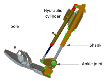
Figure 1: Structure of ankle and shank. The flexion/extension freedom is driven by a cylinder.

Neural networks have been found to be very useful for estimating nonlinear functions due to its powerful approximation capabilities. For this reason, neural networks are widely used in the context of adaptive control. An adaptive control of a class of nonlinear systems has been presented in [15] and the robustness of the closed-loop system has been proven. In [36], neural network based adaptive control has been extended to the active suspension system with actuator saturation. Adaptive neural control of nonlinear systems with nonsmooth actuator nonlinearity has been considered in [37] and a stable neural network observer has been developed in [1]. However, most of the works prescribed need the assumption that the function to be approximated by neural network is continuous. In this work, with resorting to the techniques described in  [29, 23], we extend the discussion to approximation and compensation for piecewise discontinuous function within the proposed control framework.
Another challenge of control of hydraulic actuated exoskeleton is how to compensate for the input saturation caused by the hydraulic actuator, which in principle might lead to poor tracking performance, including longer period of transient, unacceptable overshoot, even larger tracking error. To deal with this problem, many methods have been proposed, see for instance [10, 16]. Among them, an auxiliary system has been introduced in [16] for the impedance control of a robotic manipulator subject to input saturation. In [17], an adaptive control of mobile robot with torque saturation has been studied. The torque has been designed to be a function constructed by model parameter that can be guaranteed within the saturation limit. In [33], an iterative learning control approach has been proposed for nonlinear uncertain systems, of which the convergence of the state has been proven under control saturation. A PID controller has been used to control robot manipulators under bounded torque saturation with exponential stability property guaranteed using singular perturbation theory, see [28]. Inspired by above techniques, in this work a Lyapunov-based virtual system is introduced to compensate for the control saturation, where its model terms and parameters are properly designed according to Lyapunov direct method.
Fig. 1 depicts a left ankle joint equipped with a hydraulic actuator. The control problem of such a lower-limb exoskeleton is addressed in this work. Note that, as the control of one joint can be easily extended to that of the whole exoskeleton system, for simplicity, only the control problem of an ankle joint is considered in this work.
To be specific, a two-layer Lyapunov-based adaptive cascade control scheme for joint position control of a lower-limb exoskeleton is presented. Its control diagram is depicted in Figure 2. At the higher layer of the control structure, a Lyapunov-based adaptive regulator is designed for the leg dynamics including adaptation algorithms for uncertain parameters and friction estimations, with the goal of minimizing the deviation of the joint position $\varphi$ and its reference value $\varphi_{d}$. The outcome of this layer is the desired value of the hydraulic actuator force reference $F_{L,d}$ to be followed at the low level. At the lower layer, a Lyapunov-based neural network adaptive regulator computes the input signal $u$ for the hydraulic exoskeleton system with the scope of tracking the desired force $F_{L,d}$, meanwhile compensates for the unknown time-varying parameter and piecewise discontinuous nonlinearity with an integrated neural network composed by both continuous and discontinuous basis functions, and for control saturation with an auxiliary virtual system. The proposed approach shows to be capable in minimizing the interaction torque between machine and human, and suitable for imprecise models.

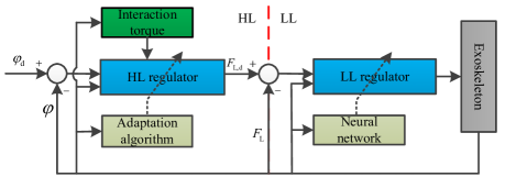
Figure 2: Diagram of the proposed control scheme. HL=Higher layer, LL=Lower layer.

The overall robustness property of the two levels is analyzed under input constraint. Simulation experiments including a comparison with PD controller are reported, so as to verify the effectiveness of the proposed approach in reference tracking and in interaction torque minimization, and its potentiality for control of models with uncertainty and nonlinearity.
The main contributions of this work are summarized as follows:

• The adopted cascade structure can improve the control performance with respect to the single layer control scheme when there exists model uncertainty and/or exogenous disturbance affecting directly the lower layer system. In this case, the proposed algorithm can indeed limit the effects caused by the uncertainty and/or disturbance at the lower layer on the controlled variables at the higher layer.

• The approach allows for multi-objectives at the high layer, e.g., the minimization of the joint position tracking error and the optimization of the interaction torque between machine and human.

• The synthesis of continuous RBF and discontinuous jump approximate function are used to estimate piecewise discontinuous function caused by system nonlinearity and friction force.

• The proposed control scheme shows to be suitable for systems with possibly multiple unknown (possibly time-varying) parameters and nonlinear functions.

The rest of the paper is organized as follows. In Section  2 the model is described and the control goal is introduced. The design of the high-level and low-level Lyapunov-based adaptive controller is presented in Sections 3 and 4, respectively, while the closed-loop properties are described in Section 5. The simulation results are reported in Section 6, while some conclusions are drawn in Section 7.

2 System description and control objective

In this section the nonlinear model of the overall system under study and the main idea to deal with the control problem are described.

2.1 System description

The ankle joint of the exoskeleton is driven by a hydraulic servo system, and its schematic diagram is depicted in Fig. 3. The operating principle of the hydraulic system is as follows. When the relay is closed, high-pressure oil from the pump flows through the check valve into the accumulator in case the gas pressure of the accumulator is smaller than the oil pressure. Meanwhile, a second flow direction is made where the oil flows through the left hole of the four-sided servo valve into the left (right) chamber of the valve core. The oil then flows through the servo valve to the actuator in order to drive an external load. Notice that, the measured force of the cylinder from the force sensor is transmitted to the regulator such that the control action applied to the actuator is computed according to the error of the desired force and the measured one. Valve openings are changeable according to the input signal computed with the controller. This determines the values of pressure and flow in the acting chamber of the actuator.

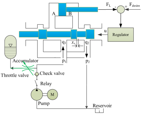
Figure 3: The hydraulic system contains: a reservoir, pump, throttle valve, relay, check valve, accumulator, four-sided servo valve and cylinder.

It is highlighted that the accumulator is designed to supply oil in place of the pump when the relay is open, with the objective of saving energy and prolonging the working time. The throttle valve is selected to guarantee the flow coming from (going into) the accumulator remaining almost constant.
To sum up, there are two working modes for the hydraulic system.

• Mode 1: The relay switches on. In this case, the pump provides oil for the system, in the meanwhile, charges the accumulator with oil. Once the pressure of the accumulator reaches its high threshold value, the relay switches off, and the pump stops working.

• Mode 2: The relay switches off. In this case, the accumulator persistently releases energy so as to provide oil to the system. Once the pressure of accumulator reaches its low threshold value (minimum working limitation value), the relay switches on, and the whole system goes back to Mode 1.

The oil flow-rate of the four-sided servo valve is given by

$$q_{L}=K_{q}x_{v}-K_{c}P_{L}$$ (1)

where $K_{q}$, $K_{c}$, and $x_{v}$ are the idle flow gain coefficient, the flow-pressure coefficient and the spool position of servo valve respectively; while $P_{L}$ is the hydraulic pressure associated with the external load. Under the assumption that the compressibility of the fluid is zero, the flow balancing equation in the cylinder is simplified as

$$q_{L}=\frac{1}{2}(q_{1}+q_{2})$$ (2)

where $q_{1}$ and $q_{2}$ are the flow rates into chambers A and B respectively.
Furthermore, it also holds that

$$q_{1}= {C_{in}}(P_{1}-P_{2})+{C_{ec}}{P_{1}}+\dot{\mathcal{V}}_{1}+\frac{{{{\mathcal{V}}_{1}}}}{\beta}{\dot{P}_{1}}$$ (3a)

$$q_{2}= {C_{in}}(P_{1}-P_{2})-{C_{ec}}{P_{2}}-\dot{\mathcal{V}}_{2}-\frac{{{{\mathcal{V}}_{2}}}}{\beta}{\dot{P}_{2}}$$ (3b)

where $A_{1}$, $P_{1}$, and ${\mathcal{V}}_{1}$ are the area of piston, the hydraulic pressure and the volume in chamber A, while $A_{2}$, $P_{2}$, and ${\mathcal{V}}_{2}$ are the corresponding counterpart in chamber B. $\beta$ is the effective bulk modulus. $C_{in}$ and $C_{ex}$ are the cylinder internal and external leakage coefficients. $\dot{P}_{i}$ and $\dot{\mathcal{V}}_{i}$ are the derivatives of $P_{i}$ and ${\mathcal{V}}_{i}$, $i=1,2$.
The hydraulic pressures of chamber A and B satisfy

$$P_{L}= P_{1}-P_{2}$$ (4a)

$$P_{s}= P_{1}+P_{2}$$ (4b)

where $P_{s}$ is the outlet oil pressure of the pump and $P_{L}$ is the pressure associated with the external load. Assuming that $P_{s}$ is derivable, from (4), it holds that

$$\dot{P}_{1}= \frac{\dot{P}_{L}+\dot{P}_{s}}{2}$$ (5a)

$$\dot{P}_{2}= \frac{\dot{P}_{L}-\dot{P}_{s}}{2}$$ (5b)

The volume ${\mathcal{V}}_{i}$, $i=1,2$, respect the geometric principle, i.e.,

$${\mathcal{V}}_{1}= {\mathcal{V}}_{0}+A_{1}x_{c}$$ (6a)

$${\mathcal{V}}_{2}= {\mathcal{V}}_{0}-A_{2}x_{c}$$ (6b)

where $x_{c}$ is the piston position of the cylinder.
In view of (1)-(6), the cylinder flow reads

$${q_{L}}=\frac{{{A_{1}}+{A_{2}}}}{2}{\dot{x}_{c}}+({{C_{in}}+{C_{ec}}}){P_{L}}+\frac{{{{\mathcal{V}}_{0}}}}{{2\beta}}{\dot{P}_{L}}$$ (7)

where $\dot{x}_{c}$ is the piston velocity of the cylinder.
The mathematical model of the accumulator is presented as

$${P_{0}}{\mathcal{V}}_{0}^{r_{0}}={P_{h}}{\mathcal{V}}_{h}^{r_{0}}={P_{l}}{\mathcal{V}}_{l}^{r_{0}}$$ (8)

where $r_{0}>1$ is a constant value, $P_{h}$ and $P_{l}$ are the corresponding high and low threshold values of pressure in the accumulator. The high threshold value is chosen as $P_{h}=P_{p}$, where $P_{p}$ is the outlet oil pressure of the pump; ${\mathcal{V}}_{h}$ and ${\mathcal{V}}_{l}$ are the associated gas volume. Assuming that the relay switches off at a generic time instant $t$, the future pressure in the accumulator drops till it reaches the low threshold value, see Fig. 4. Thanks to the use of throttle valve, the inlet (outlet) flow of the accumulator can be assumed to be constant, then the pressure satisfies

$$P_{t+\Delta t}=P_{h}\left({\frac{{{{\mathcal{V}}_{h}}}}{{{{\mathcal{V}}_{h}}+{q_{a}}\cdot\Delta t}}}\right)^{r_{0}}$$ (9)

where $q_{a}$ is the inlet (outlet) flow of the accumulator. Therefore, the working pressure during the two modes can be represented as

$${P_{s}}=\left\{\begin{array}[]{ll}{P_{p}},&\text{Mode1}\\ {P_{t+\Delta t}},&\text{Mode2}\end{array}\right.$$ (10c)

Moreover, its derivative is defined as

$${\dot{P}_{s}}=\left\{\begin{array}[]{ll}0,&\text{Mode1}\\ {\dot{P}_{t+\Delta t}},&\text{Mode2}\end{array}\right.$$ (10f)

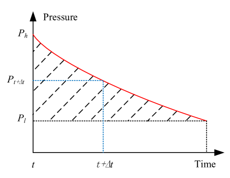
Figure 4: The relationship between the pressure and the working time $\Delta t$ of the accumulator.

By inspecting the motion function of the actuator, the force that drives the external load is given in the form of

$$F_{L}=A_{1}P_{1}-A_{2}P_{2}$$ (11)

Recalling the structure of the leg (see again Fig. 1), the output force $F_{L}$ of the hydraulic servo system acts as the control input for the inverted pendulum model of the leg dynamics, which is represented as (see  [27])

$$J\ddot{\varphi}+mgr\sin(\varphi)=N({F_{L}}+{F_{f}})+\tau_{hm}$$ (12)

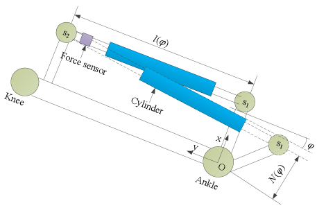
Figure 5: Kinematical structure of the actuated shank.

where $\varphi$ is the joint angle of the ankle, $J$ is the inertia of the shank, $N$ is the actuator moment arm (see Fig. 5), $m$ is the mass of the shank, $r$ is the center position of the mass of the shank, $F_{f}$ is the friction force of the piston. $\tau_{hm}$ is the interaction torque between machine and human described by

$$\tau_{hm}=k_{p}(\varphi-\varphi_{d})+k_{d}(\dot{\varphi}-\dot{\varphi}_{d})$$ (13)

where parameters $k_{p}$ and $k_{d}$ are constant values that amplify the differences of the angles and their velocities between machine and human. The joint angle of the ankle establishes a relationship with the position of the piston, that is

$$x_{c}=l(\varphi)-l_{0}-x_{c0}$$ (14)

where $l_{0}$ is the initial length of the cylinder, $x_{c0}$ is the initial position of the piston, $l(\varphi)$ is the length of the cylinder that can be calculated according to the geometrical analysis of the shank as shown in Fig. 5. To this end, first note that the cylinder is placed between the ankle joint and the knee joint mounting at the points $s_{1}$ and $s_{2}$, and $O$ is the origin of the coordinates for the ankle joint. Denoting by $r_{s1}$ and $r_{s2}$ the distance from $s_{1}$ and $s_{2}$ to the coordinate origin, the length of the cylinder $l(\varphi)$ can be computed according to Law of cosines, that is

$$l(\varphi)=\sqrt{-2r_{s1}r_{s2}cos(\varphi-\theta_{1}-\theta_{2})+r_{s1}^{2}+r_{s2}^{2}}$$ (15)

where $\theta_{1}=tan^{-1}(a_{1}/-b_{1})$, $\theta_{2}=tan^{-1}(a_{2}/b_{2})$, $a_{1}$, $a_{2}$ are the coordinate positions of $s_{1}$ and $s_{2}$ along the $x$ axis, while $b_{1}$ and $b_{2}$ are the coordinate positions of $s_{1}$ and $s_{2}$ along the $y$ axis respectively. The moment arm in (12) is a function of $l(\varphi)$:

$$N=r_{d1}\text{sin}(\text{cos}^{-1}(\frac{r_{d2}^{2}-l(\varphi)^{2}-r_{d1}^{2}}{-2l(\varphi)r_{d1}}))$$ (16)

The friction force in the hydraulic cylinder is not negligible and can be composed by Coulomb force, Viscous force, Stribeck effects and position dependent forces, see [5, 8]. However, it has been noticed that the Stribeck effects and the position dependent forces are usually very small, thus for simplicity, they are neglected in this case. The friction model of the piston is given by

$${F_{f}}=-F_{C}\operatorname{sgn}({\dot{\varphi}})-b{\dot{\varphi}}$$ (17)

where $F_{C}$ and $b$ are the Coulomb friction term and the viscous friction coefficient respectively.
The input to the hydraulic servo system is the electrical current, that affects directly the spool position through the mechanical time constant $\tau$ and the DC gain of the valve current $k_{s}$ to the spool position $x_{v}$. This relationship is described as

$$\dot{x}_{v}=\frac{1}{\tau}(k_{s}u-x_{v})$$ (18)

It is usually unavoidable in servo valve that the input is saturated by its maximum and minimum limits, see for instance [35]. The control saturation of the actuator can be described by

$$u=\left\{\begin{array}[]{lc}u_{max}&u>u_{max}\\ u&u_{min}\leq u\leq u_{max}\\ u_{min}&u<u_{min}\end{array}\right.$$ (19)

where $u_{min}\leq u_{max}$. If the computed value of the control variable violates the constraint $\begin{bmatrix}u_{min}&u_{max}\end{bmatrix}$, control saturation occurs and the input is partially applied to (18). The residual input that can not be implemented is defined as $\delta$ and is represented by [10]

$$\delta=\left\{\begin{array}[]{lc}u_{max}-u&u>u_{max}\\ 0&u_{min}\leq u\leq u_{max}\\ u_{min}-u&u<u_{min}\end{array}\right.$$ (20)

In view of (7)-(18), one can write the system in the state-space form

$$\Sigma:\left\{\begin{array}[]{l}\ddot{\varphi}=\frac{1}{J}(N({F_{L}}+{F_{f}})-mgr\sin(\varphi)+\tau_{hm})\\ {\dot{F}}_{L}={n_{1}}{x_{v}}-{n_{2}}{{\dot{x}}_{c}}-{n_{3}}{F_{L}}+{n_{4}}{P_{s}}+n_{5}\dot{P}_{s}\\ {{\dot{x}}_{v}}=\frac{1}{\tau}({k_{s}}u-{x_{v}})\end{array}\right.$$ (21)

where

$${n_{1}}=\frac{{2\beta({A_{1}}+{A_{2}}){K_{q}}}}{{{2{\mathcal{V}}_{0}+(A_{1}-A_{2})x_{c}}}},\ {n_{2}}=\frac{{\beta{{({A_{1}}+{A_{2}})}^{2}}}}{{2{\mathcal{V}}_{0}+(A_{1}-A_{2})x_{c}}},$$

$${n_{3}}=\frac{{2\beta(2{K_{c}}+{2C_{in}}+{C_{ex}})}}{{2{\mathcal{V}}_{0}+(A_{1}-A_{2})x_{c}}},\ {n_{4}}=\frac{{\beta(2{K_{c}}+2{C_{in}}+{C_{ex}})({A_{2}}-{A_{1}})}}{{2{{\mathcal{V}}_{0}}+(A_{1}-A_{2})x_{c}}},$$

$$n_{5}=\frac{A_{2}-A_{1}}{2}-\frac{{{{({A_{1}}+{A_{2}})}^{2}}}}{{2(2{\mathcal{V}}_{0}+(A_{1}-A_{2})x_{c})}}.$$

2.2 Control objective

Considering a reference trajectory $\varphi_{d}$ for the angle variable of the ankle joint and denoting $e_{1}$ the deviation of the value of the real angle and the desired one, i.e.,

$$e_{1}=\varphi-\varphi_{d}$$ (22)

the control goal for system (21) is to drive $e_{1}$ to the origin. The control problem is trivial if the system (21) is precise. In fact, the system (21) is a simplified representation especially for the hydraulic servo model. Moreover, the mass $m$ and the inertia $J$ of the inverted pendulum model (12) are usually difficult to be accurately measured. For these reasons, adaptive control algorithms that estimate the constant and time-varying parameters, and compensates for the friction force, neglected nonlinearity, and time-varying pressure supply, can be used so as to achieve the aforementioned control goal. Note also that, the model (21) can be partitioned into a hierarchical structure, where the high-level dynamic is

$$\Sigma_{H}:\ddot{\varphi}=\frac{1}{J}(N({F_{L}}+{F_{f}})-mgr\sin(\varphi)+\tau_{hm}),$$ (23a)

while the low-level model is given as

$$\Sigma_{L}:\left\{\begin{array}[]{l}{\dot{F}}_{L}={n_{1}}{x_{v}}-{n_{2}}{{\dot{x}}_{c}}-{n_{3}}{F_{L}}+{n_{4}}{P_{s}}+n_{5}\dot{P}_{s}\\ {{\dot{x}}_{v}}=\frac{1}{\tau}({k_{s}}u-{x_{v}})\end{array}\right.$$ (23d)

It can be noted that, (23) coincides with the cascade model structure in which, the variable $F_{L}$ acts as the input to $\Sigma_{H}$ and as one of the outputs to $\Sigma_{L}$, establishing a direct interconnection between the two subsystems. As previously described, in principle, a single-layer adaptive controller can be designed regarding (23) as a whole. However, in this way, the closed-loop control performance might be sensitive to model uncertainty and disturbance. In view of this, the proposed solution in this note is an adaptive Lyapunov-based approach with hierarchical cascade control structure. This control approach naturally corresponds to the model structure, with which, the influence of possible uncertainty and nonlinearity from $\Sigma_{L}$ to $\Sigma_{H}$ can be suppressed, e.g., via properly designed compensation algorithm at the low level. A brief description of the controller at the two levels is as follows. The higher layer regulator is in charge of computing the required value of $F_{L}$ for (23a) such that the goal $E=e_{1}^{\top}e_{1}$ is minimized. The constant unknown parameters, e.g. the mass $m$, and the inertia $J$, are properly estimated, and the friction force is accounted for. At the lower layer, the regulator is designed for (23d) with the scope to track the force $F_{L}$ computed at the higher layer and to compensate for the possible uncertainty and nonlinearity. The following standard assumption is assumed to be holding:

Assumption 1

The cylinder force $F_{L}$, ankle joint angle $\varphi$, velocity $\dot{\varphi}$, and the accelerated velocity $\ddot{\varphi}$ are measurable.

3 Design of the high-level Lyapunov-based adaptive controller

In this section, the high-level Lyapunov-based controller is designed and the adaptive parameters estimation algorithms are introduced with the objective to drive $e_{1}$ to the origin.

3.1 High-level Lyapunov-based controller

First, denoting $x_{1}=\varphi$, $x_{2}=\dot{\varphi}$, rewrite the model (23a) as

$$\Sigma_{H}:\left\{\begin{array}[]{l}\dot{x}_{1}=x_{2}\\ \dot{x}_{2}=\frac{1}{J}(N({F_{L}}+{F_{f}})-mgr\sin(x_{1})+\tau_{hm})\end{array}\right.$$ (24)

In view of (22), define a virtue control variable $v_{1}=-k_{1}e_{1}+\dot{\varphi_{d}}$, $k_{1}>0$ and denote

$$e_{2}=x_{2}-v_{1}=k_{1}e_{1}+(\dot{\varphi}-\dot{\varphi}_{d})$$ (25)

By applying the concept of back-stepping control (see [9]), we define a new system corresponding to (24) in the following form:

$$\Sigma_{H}:\left\{\begin{array}[]{l}\dot{e}_{1}=-k_{1}e_{1}+e_{2}\\ \dot{e}_{2}=\frac{1}{J}(N({F_{L}}+{F_{f}})-mgr\sin(x_{1})+\tau_{hm})-\dot{v}_{1}\end{array}\right.$$ (26)

In order to design a proper Lyapunov-based controller, as consider the following Lyapunov function

$$V_{H,1}=\frac{1}{2}\rho_{1}e_{1}^{2}+\frac{1}{2}\rho_{2}Je_{2}^{2}$$ (27)

where $\rho_{1}>0$, $\rho_{2}>0$ are the penalty weights associated with $e_{1}$ and $e_{2}$ respectively. Taking the derivative of $V_{H,1}$ in (27), one has

$$\begin{array}[]{rll}&\dot{V}_{H,1}=\rho_{1}e_{1}(-k_{1}e_{1}+e_{2})+\rho_{2}Je_{2}(\dot{x}_{2}-\dot{v}_{1}(t))\\ &=-k_{\rho_{1}}e_{1}^{2}-k_{\rho_{2}}e_{2}^{2}+\\ &\rho_{2}e_{2}\underbrace{(k_{2}e_{2}+\rho_{12}e_{1}+N(F_{L}+F_{f})-mgrsin(x_{1})+\tau_{hm}-J\dot{v}_{1})}\\ &\ \ \ \ \ \ \ \ \ \ \ \ \ \ \ \ \ \ \ \ \ \ \ \ \ \ \ \ \ \ \ \ \ \ \ \ \ \ \ \ \ \ \ \ \ \text{set}=0\end{array}$$

where $k_{2}>0$, $k_{\rho_{1}}=k_{1}\rho_{1}$, $k_{\rho_{2}}=k_{2}\rho_{2}$, and $\rho_{12}=\rho_{1}/\rho_{2}$.
Therefore, the control action can be selected as

$$F_{L}=-\frac{1}{N}(k_{2}e_{2}+\rho_{12}e_{1}+NF_{f}+\tau_{hm}-mgrsin(x_{1})-J\dot{v}_{1})$$ (28)

such that $\dot{V}_{H,1}=-k_{\rho_{1}}e_{1}^{2}-k_{\rho_{2}}e_{2}^{2}\leq 0$. where $k_{\rho_{1}}$ and $k_{\rho_{2}}$ are the tuning knobs taht define the decaying rate of the Lyapunov function $V_{H,1}$.

Remark 1

In view of the definition of $\tau_{hm}$ in (12) and $e_{2}$ in (25), if parameter $k_{1}$ is selected such that $k_{1}=k_{p}/k_{d}$, one promptly has $e_{2}=\tau_{hm}/k_{d}$. In this case, it is easy to see that the interaction torque $\tau_{hm}$ can also be minimized via the second term in the right-hand side of (27).

3.2 Adaptive design with the estimations of $m$ and $J$

The input defined in (28) is highly model dependent that the mass $m$ and the inertia $J$ are assumed to be accurately measured which however in principle is nontrivial in practical situation. In view of this, an adaptive update algorithm is proposed to estimate $m$ and $J$. To this end, denote by $\hat{m}$ and $\hat{J}$ the estimated values of $m$ and $J$, and by $\tilde{m}=m-\hat{m}$ and $\tilde{J}=J-\hat{J}$ the corresponding estimation errors. Consider the following augmented Lyapunov function as

$$V_{H,2}=V_{H,1}+\frac{1}{2}q_{J}\tilde{J}^{2}+\frac{1}{2}q_{m}\tilde{m}^{2}$$

where $q_{J}$ and $q_{m}$ are positive scalars. A new control action in place of (28) is selected by substituting the corresponding estimated values for $m$ and $J$, i.e.,

$$F_{L}=-\frac{1}{N}(k_{2}e_{2}+\rho_{12}e_{1}+NF_{f}+\tau_{hm}-\hat{m}grsin(x_{1})-\hat{J}\dot{v}_{1})$$ (29)

Taking the derivative of $V_{H,2}$ and applying the input (29), one has

$$\begin{array}[]{l}\dot{V}_{H,2}=\\ =-k_{\rho_{1}}e_{1}^{2}-k_{\rho_{2}}e_{2}^{2}-\rho_{2}e_{2}(\tilde{m}grsin(x_{1})+\tilde{J}\dot{v}_{1})-q_{J}\tilde{J}\dot{\hat{J}}-q_{m}\tilde{m}\dot{\hat{m}}\\ =-k_{\rho_{1}}e_{1}^{2}-k_{\rho_{2}}e_{2}^{2}-\tilde{J}\underbrace{(\rho_{2}e_{2}\dot{v}_{1}+q_{J}\dot{\hat{J}})}-\tilde{m}\underbrace{(\rho_{2}e_{2}grsin(x_{1})+q_{m}\dot{\hat{m}})}\\ \ \ \ \ \ \ \ \ \ \ \ \ \ \ \ \ \ \ \ \ \ \ \ \ \ \ \ \ \ \ \ \ \ \ \ \ \ \ \ \ \text{set}=0\ \ \ \ \ \ \ \ \ \ \ \ \ \ \ \ \ \ \ \ \ \ \ \ \ \text{set}=0\end{array}$$

The parameter adaptation algorithm of $\hat{J}$ and $\hat{m}$ can be chosen as

$$\dot{\hat{J}}= -\frac{1}{q_{J}}\rho_{2}e_{2}\dot{v}_{1}$$ (30a)

$$\dot{\hat{m}}= -\frac{1}{q_{m}}\rho_{2}e_{2}grsin(x_{1})$$ (30b)

Thus, under the control choice (29) and the estimation updating rule (30), it holds that

$$\dot{V}_{H,2}=-k_{\rho_{1}}e_{1}^{2}-k_{\rho_{2}}e_{2}^{2}.$$

3.3 Adaptive design with friction force estimation

In the previous section 3.2, model (17) is included in the proposed control action for the objective of friction force compensation. Notice that, the parameters of the friction model can be obtained according to repeated experiments validation, see [3]. In this work, instead, we propose an adaptation algorithm to estimate the parameters of friction force within the structure of (17). In doing so, the cumbersome experiment validation can be avoided. To this end, define the corresponding estimated friction force as

$${\hat{F}_{f}}=-{\hat{F}_{C}}\operatorname{sgn}({\dot{\varphi}})-\hat{b}{\dot{\varphi}}$$ (31)

where $\hat{F}_{C}$ and $\hat{b}$ are the estimated values of $F_{C}$ and $b$ respectively. Considering the estimated friction force as one of the feedback terms, the control action is amended as

$$F_{L}=-\frac{1}{N}(k_{2}e_{2}+\rho_{12}e_{1}+N\hat{F}_{f}+\tau_{hm}-\hat{m}grsin(x_{1})-\hat{J}\dot{v}_{1})$$ (32)

Accordingly, a new Lyapunov candidate is considered in the form

$$V_{H,3}=V_{H,2}+\frac{1}{2}q_{C}\tilde{F}_{C}^{2}+\frac{1}{2}q_{b}\tilde{b}^{2}$$

where $\tilde{F}_{C}=F_{C}-\hat{F}_{C}$ and $\tilde{b}=b-\hat{b}$; $q_{C}$ and $q_{b}$ are positive scalars.
Taking the derivative of $V_{H,3}$ and applying the control action (32), it holds that

$$\dot{V}_{H,3}=-k_{\rho_{1}}e_{1}^{2}-k_{\rho_{2}}e_{2}^{2}+\rho_{2}Ne_{2}(F_{f}-\hat{F}_{f})-q_{C}\tilde{F}_{C}\dot{\hat{F}}_{C}-q_{b}\tilde{b}\dot{\hat{b}}$$

In view of (17) and (31), one has

$$\begin{array}[]{ll}\dot{V}_{H,3}=&-k_{\rho_{1}}e_{1}^{2}-k_{\rho_{2}}e_{2}^{2}-\rho_{2}Ne_{2}\tilde{F}_{C}\operatorname{sgn}({\dot{\varphi}})-\\ &\rho_{2}Ne_{2}\tilde{b}{\dot{\varphi}}-q_{C}\tilde{F}_{C}\dot{\hat{F}}_{C}-q_{b}\tilde{b}\dot{\hat{b}}\end{array}$$

By using the associative law of addition in polynomials, then one has

$$\begin{array}[]{lll}\dot{V}_{H,3}=&-k_{\rho_{1}}e_{1}^{2}-k_{\rho_{2}}e_{2}^{2}-\tilde{F}_{C}\underbrace{(\rho_{2}Ne_{2}\operatorname{sgn}{\dot{\varphi}}+q_{C}\dot{\hat{F}}_{C})}-\\ &\ \ \ \ \ \ \ \ \ \ \ \ \ \ \ \ \ \ \ \ \ \ \ \ \ \ \ \ \ \ \ \ \ \ \ \ \ \ \ \ \ \ \ \ \ \text{set}=0\\ &\tilde{b}\underbrace{(\rho_{2}Ne_{2}\dot{\varphi}+q_{b}\dot{\hat{b}})}.\\ &\ \ \ \ \ \ \ \ \ \ \text{set}=0\end{array}$$ (33)

Therefore, the adaptation algorithm for parameters $\hat{F}_{C}$ and $\hat{b}$ are selected as follows:

$$\dot{\hat{F}}_{C}= -\frac{1}{q_{C}}\rho_{2}Ne_{2}\operatorname{sgn}{\dot{\varphi}}$$ (34a)

$$\dot{\hat{b}}= -\frac{1}{q_{b}}\rho_{2}Ne_{2}\dot{\varphi}$$ (34b)

Remark 2

It is worth mentioning that, as the right-hand sides of the adaptation algorithm (34a) and $\dot{e}_{2}$ with (26) are piecewise affine on the state variables, the uniqueness solution condition of the resultant closed-loop system might not be verified, see [21]. Therefore, the usage of the Lyapunov stability theorem, such as LaSalle’s theorem, for the stability analysis of (26) is not straightforward. Nevertheless, we show in the following that the corresponding convergence property can be proven in the Filippov sense, see [30, 14].

Theorem 1

With the control action (32), and the adaptation algorithms (30) and (34), the closed-loop form of (26) is asympotically stable, that the tracking error $e_{1},\,e_{2}$ converge to the origin as time goes to infinity.

Proof 1

With (32), (30), and (34), it is possible to write the closed-loop form, of which we highlight that, in addition to that of (34a), the right-hand side of $\dot{e}$ is also piecewise affine on the state variables due to (32). To show the convergence of $e_{1}$, $e_{2}$, we have to check the monotonicity of the Lyapunov function $V_{H,3}$ for all the Filippov solutions. To proceed, we split the state variables into two regions: $\mathcal{Z}_{1}=\{z\in\mathbb{R}^{6}|e_{2}<-\dot{\varphi}_{d}\}$, $\mathcal{Z}_{2}=\{z\in\mathbb{R}^{6}|e_{2}>-\varphi_{d}\}$, and a separating surface between $\mathcal{Z}_{1}$ and $\mathcal{Z}_{2}$, that is $\mathcal{Z}_{3}=\{z\in\mathbb{R}^{6}|e_{2}=-\varphi_{d}\}$, where $z=\begin{bmatrix}e_{1}&e_{2}&\hat{J}&\hat{m}&\hat{F}_{C}&\hat{b}\end{bmatrix}^{\top}$. In view of this, we first show that, for $z\in\mathcal{Z}_{1},\,or\,\mathcal{Z}_{2}$, the term $sgn(\dot{\varphi})$ can be replaced by constant values, which verifies the smoothness of the closed-loop system. Thus, the derivative of $V_{H,3}$ can be easily computed, i.e., $\dot{V}_{H,3}=-k_{\rho_{1}}e_{1}^{2}-k_{\rho_{2}}e_{2}^{2}$. For the case $z\in\mathcal{Z}_{3}$, i.e., when the sliding motion might occurs, $sgn(\dot{\varphi})=0$ leads to $\hat{F}_{C}=\emph{constant}$, to the smoothness of the closed-loop system, and to $\dot{V}_{H,3}=-k_{\rho_{1}}e_{1}^{2}-k_{\rho_{2}}e_{2}^{2}$. To sum up, for almost all $t$, and $\forall\,z$,

$$\dot{V}_{H,3}=-k_{\rho_{1}}e_{1}^{2}-k_{\rho_{2}}e_{2}^{2},$$ (35)

which implies that $\dot{V}_{H,3}<0$ for $\begin{bmatrix}e_{1}&e_{2}\end{bmatrix}^{\top}\neq 0$ along all the Filippov solutions, thus the origin is globally stable in the Filippov sense.
Also, according to [25], from (35), it holds that, for all $t$,

$$V_{H,3}\leq\bar{V},$$ (36)

where $\bar{V}$ is an abitrarily large finite positive scalar. In view of (35) and, (36), recalling that $V_{H,3}$ is differentiable and the right-hand sidde term $-k_{\rho_{1}}e_{1}^{2}-k_{\rho_{2}}e_{2}^{2}$ is smooth, by Barbalat’s Lemma, the variables $e_{1}$ and $e_{2}$ converge to the origin respectively as time goes to infinity. $\square$

In view of Theorem 1, the control goal is achieved, i.e., the angle $\varphi$ converges to its desired value $\varphi_{d}$. Furthermore, in view of the definition of $e_{2}$, it follows that the angle velocity $\dot{\varphi}$ converges to $\dot{\varphi}_{d}$. Note that, it is not guaranteed that the estimated value $\hat{m}$, $\hat{J}$, $\hat{F}_{C}$, and $\hat{b}$ will converge to their true values. It is because their true values are usually unknown, thus the differences with respect to their estimated values are not available at all times and can not guarantee to be exactly compensated via adding feedback error terms in the corresponding adaptation laws. Even so, this fact does not make any negative influence on the convergence of $e_{1}$ and $e_{2}$. The desired trajectory of $F_{L}$ to be tracked by the low-level controller is given as

$$F_{L,d}=-\frac{1}{N}(k_{2}e_{2}-\rho_{12}e_{1}+N\hat{F}_{f}+\tau_{hm}-\hat{m}grsin(x_{1})-\hat{J}\dot{v}_{1})$$ (37)

$F_{L,d}$ is a reasonable choice for the reference signal of the low layer for the reason that $e_{1}$ and $e_{2}$ can always be measured in real-time and the unknown parameters are replaced with estimated ones that are adaptively updated by the proper design at the high layer.

4 Devise of the low-level Lyapunov-based neural network adaptive regulator

In this section, the low-level Lyapunov-based regulator with the neural-network based estimation algorithm is designed for (23d), with the objective to track the reference signal $F_{L,d}$ computed at the high layer, and to compensate for unknown time-varying parameters and nonlinear piecewise discontinuous function.

4.1 Low-level Lyapunov-based regulator

First note that the friction force model contains the $\operatorname{sgn}(\dot{\varphi})$ term, thus it is not derivable in the domain $\dot{\varphi}=0$. For this reason, we define by $\dot{\hat{F}}_{f}$ an approximated derivative function associated with ${\hat{F}}_{f}$, i.e.,

$$\dot{\hat{F}}_{f}=\left\{\begin{array}[]{ll}\dot{\hat{F}}_{f}^{+},&\dot{\varphi}\geq\epsilon_{0}\\ \frac{-\hat{F}_{C}-\hat{b}\epsilon_{0}}{\epsilon_{0}},&-\epsilon_{0}\leq\dot{\varphi}<\epsilon_{0}\\ \dot{\hat{F}}_{f}^{-},&\dot{\varphi}<\epsilon_{0}\end{array}\right.$$ (38)

where $\dot{\hat{F}}_{f}^{+}=-\hat{F}_{C}-\hat{b}\ddot{\varphi}-\dot{\hat{b}}\dot{\varphi}$, $\dot{\hat{F}}_{f}^{-}=\hat{F}_{C}-\hat{b}\ddot{\varphi}-\dot{\hat{b}}\dot{\varphi}$, $\epsilon_{0}$ is a small positive scalar, $\ddot{\varphi}$ is the second derivative of $\varphi$.

Assumption 2

Assume that $\epsilon_{0}$ is chosen small enough such that the friction force $\hat{F}_{f}$ can be properly approximated by $\int^{t}\dot{\hat{F}}_{f}$, i.e., $\hat{F}_{f}=\int^{t}\dot{\hat{F}}_{f}$.

In order to derive the model to be used at the low level, we denote $x_{3}=F_{L}$, and rewrite the system (23d) as

$$\left\{\begin{array}[]{l}\dot{x}_{3}=n_{1}x_{v}-n_{2}\dot{x}_{c}-n_{3}x_{3}+n_{4}P_{s}+n_{5}\dot{P}_{s}\\ {{\dot{x}}_{v}}=\frac{1}{\tau}({k_{s}}u-{x_{v}})\end{array}\right.$$ (39)

Thanks to the definition of $\dot{\hat{F}}_{f}$, we define by $e_{3}$ the deviation of $x_{3}$ and the desired one, i.e., $e_{3}=x_{3}-F_{L,d}$, then it is possible to write (39) as

$$\left\{\begin{array}[]{l}\dot{e}_{3}=n_{1}(x_{v}+f_{4})\\ {{\dot{x}}_{v}}=\frac{1}{\tau}({k_{s}}u-{x_{v}})\end{array}\right.$$ (40)

where $f_{4}=\frac{1}{n_{1}}(-n_{2}\dot{x}_{c}-n_{3}x_{3}-\dot{\tilde{F}}_{L,d}-\dot{\hat{F}}_{f}+n_{14}P_{s}+n_{15}\dot{P}_{s})$, ${\tilde{F}}_{L,d}={F}_{L,d}+\hat{F}_{f}$, $n_{14}=\frac{n_{4}}{n_{1}}$, $n_{15}=\frac{n_{5}}{n_{1}}$. In the following, the aim is to design the Lyapunov-based controller for the low-level system (40) with the objective of minimizing the deviation of $F_{L}$ and $F_{L,d}$. To this end, first consider the following Lyapunov candidate

$$V_{L,1}=\frac{\rho_{3}}{2n_{1}}e_{3}^{2}$$

where $\rho_{3}>0$. Taking the derivative of $\dot{V}_{L,1}$ leads to

$$\dot{V}_{L,1}=-k_{\rho_{3}}e_{3}^{2}+\rho_{3}e_{3}(k_{3}e_{3}+x_{v}+f_{4})$$ (41)

where $k_{3}$ is chosen as a positive scalar, and $k_{\rho_{3}}=k_{3}\rho_{3}$.
As the input variable $u$ did not appear in (41), the second derivative of $V_{L,1}$ might be needed if back-stepping method is used at this level. However, note that the term $\dot{\hat{F}}_{f}$ is not continuous by the definition in (38), moreover, $n_{5}P_{s}$ is piecewise at the switching time instant from Mode 1 to Mode 2. For this reason, the back-stepping method is not advisable in this case.
To solve this problem, stabilizing $e_{3}$, the spool position in (41) has to be set equal to

$$x_{v}=-(k_{3}e_{3}+f_{4})$$ (42)

As the valve dynamics ${{\dot{x}}_{v}}=\frac{1}{\tau}({k_{s}}u-{x_{v}})$ is linear, stable, and fast, it is reasonable to assume that the input $u$ is proportional to the spool position $x_{v}$, i.e., $\dot{x}_{v}=0$, that is

$$u=\frac{1}{k_{s}}x_{v}$$ (43)

Substituting (43) into (42) gives the choice of the input variable, i.e.,

$$u=-\frac{1}{k_{s}}(k_{3}e_{3}+f_{4})$$ (44)

Considering the real dynamics ${{\dot{x}}_{v}}=\frac{1}{\tau}({k_{s}}u-{x_{v}})$, with (44), (41) can be rewritten as

$$\begin{array}[]{l}\dot{V}_{L,1}=-k_{\rho_{3}}e_{3}^{2}+\rho_{3}e_{3}(k_{3}e_{3}+(k_{s}u-\tau\dot{x}_{v}))\end{array}$$

In view of (44), one has

$$\begin{array}[]{ll}\dot{V}_{L,1}&=-k_{\rho_{3}}e_{3}^{2}-\rho_{3}e_{3}\tau\dot{x}_{v}\end{array}$$

4.2 Adaptive neural-network based estimation of $f_{4}$

Notice that the term $f_{4}$ in (40) contains nonlinearity, discontinuity, and possible uncertain time-varying parameters (e.g., $n_{1}$, $n_{2}$, $n_{3}$), thus it is nontrivial to be accurately measured or estimated with adaptation algorithms similar to the ones developed in Section 3. To properly estimate and compensate for $f_{4}$, a multi-layer neural network including both continuous RBF function and jump approximation basis function is proposed in this work.To this scope, it is highlighted that the discontinuity jump points of $\dot{\hat{F_{f}}}$ is at $\dot{\varphi}=\epsilon_{0}\,\text{and}\,-\epsilon_{0}$, while the ones of $P_{s}$ and $\dot{P}_{s}$ are at $P_{s}=P_{l}$. With above information, it is possible to write $f_{4}$ in terms of the proposed neural network in the following form:

$$f_{4}=W_{1}^{\top}h(Z)+W_{2}^{\top}\phi(Z+c_{1})+W_{3}^{\top}\phi(Z+c_{2})+\epsilon_{f}(Z)$$ (45)

where $c_{1}=\begin{bmatrix}0&\epsilon_{0}&0&P_{l}\end{bmatrix}^{\top}$, $c_{2}=\begin{bmatrix}0&-\epsilon_{0}&0&P_{l}\end{bmatrix}^{\top}$, $W_{1}\in\mathbb{R}^{n_{1}\times 1}$, $W_{2}\in\mathbb{R}^{n_{2}\times 1}$, and $W_{3}\in\mathbb{R}^{n_{2}\times 1}$, are the ideal output weight vectors, $n_{1}$ and $n_{2}$ are the corresponding numbers of the neurons, $Z=\begin{bmatrix}x_{3}&\dot{\varphi}&\dot{\tilde{F}}_{L,d}&P_{s}\end{bmatrix}^{\top}$ is the input vector, $\epsilon_{f}(Z)$ is the bounded neural network approximation error, and $h(Z)=\begin{bmatrix}h_{1}(Z)&\cdots&h_{n_{1}}(Z)\end{bmatrix}^{\top}$ is the activation function, where $h_{i}(Z)$ is selected as

$$h_{i}(Z)=\frac{(Z-\mu_{i})^{\top}(Z-\mu_{i})}{\upsilon_{i}^{2}}$$

for $i=1,\cdots,n_{1}$, where $\mu_{i}=\begin{bmatrix}\mu_{i,1}&\mu_{i,2}&\mu_{i,3}\end{bmatrix}^{\top}$ and $\upsilon_{i}$ are the center and width of the Gaussian transfer function.
The jump approximation basis function is defined as $\phi(Z)=\begin{bmatrix}\phi_{1}(Z)&\cdots&\phi_{n_{2}}(Z)\end{bmatrix}^{\top}$, where for $i=1,\cdots,n_{2}$

$$\phi_{i}(Z)=\left\{\begin{array}[]{ll}0,&\text{for}\,Z<0,\\ (1-e_{c}^{-Z})^{i},&\text{for}\,Z\geq 0\\ \end{array}\right.$$

where $e_{c}$ is the mathematical constant.
Therefore, the control variable (44) is replaced by

$$u=-\frac{1}{k_{s}}(k_{3}e_{3}+\hat{W}_{1}^{\top}h(Z)+\hat{W}_{2}^{\top}\phi(Z+c_{1})+\hat{W}_{3}^{\top}\phi(Z+c_{2}))$$ (46)

where $\hat{W}_{i}$ is the estimated values of $W_{i}$, for $i=1,2,3$. Denoting by $\tilde{W}_{i}=W_{i}-\hat{W}_{i}$, $i=1,2,3$, the corresponding estimation errors, under input (46), consider the following Lyapunov candidate

$$V_{L,2}=V_{L,1}+\frac{1}{2}\tilde{W}^{\top}\Gamma^{-1}\tilde{W}$$

where $\tilde{W}=\begin{bmatrix}\tilde{W}_{1}^{\top}&\tilde{W}_{2}^{\top}&\tilde{W}_{3}^{\top}\end{bmatrix}^{\top}$, $\Gamma=\text{diag}\{\Gamma_{1},\Gamma_{2},\Gamma_{3}\}$ is a positive definite matrix. We also denote $\hat{W}=\begin{bmatrix}\hat{W}_{1}^{\top}&\hat{W}_{2}^{\top}&\hat{W}_{3}^{\top}\end{bmatrix}^{\top}$, $\chi(Z)=\begin{bmatrix}h(Z)^{\top}&\phi(Z+c_{1})^{\top}&\phi(Z+c_{2})^{\top}\end{bmatrix}^{\top}$. Taking the derivative of $V_{L,2}$, it holds that

$$\begin{array}[]{ll}\dot{V}_{L,2}=\\ =-k_{\rho_{3}}e_{3}^{2}-\rho_{3}e_{3}\tau\dot{x}_{v}+\rho_{3}e_{3}(f_{4}-\hat{W}^{\top}\chi(Z))-\tilde{W}^{\top}\Gamma^{-1}\dot{\hat{W}}\\ =-k_{\rho_{3}}e_{3}^{2}-\rho_{3}e_{3}\tau\dot{x}_{v}+\rho_{3}e_{3}\epsilon_{f}(Z)+\rho_{3}e_{3}(\tilde{W}^{\top}\chi(Z)-\tilde{W}^{\top}\Gamma^{-1}\dot{\hat{W}}\\ =-k_{\rho_{3}}e_{3}^{2}-\rho_{3}e_{3}\tau\dot{x}_{v}+\rho_{3}e_{3}\epsilon_{f}(Z)+\tilde{W}^{\top}(\rho_{3}e_{3}\chi(Z)-\Gamma^{-1}\dot{\hat{W}})\end{array}$$

Therefore, the adaptation algorithm for $\hat{W}$ can be chosen as

$$\dot{\hat{W}}=\Gamma(\rho_{3}e_{3}\chi(Z)-\sigma\hat{W})$$ (47)

where $\sigma=\text{diag}\{\sigma_{1},\sigma_{2},\sigma_{3}\}$, is a robust matrix.

4.3 Compensation for the control saturation

Due to the control saturation described in (19), in view of the definition of $\delta$ in (20), from (46), the final control action applied to the low-level regulator is selected as

$$u=-\frac{1}{k_{s}}(k_{3}e_{3}+\hat{W}^{\top}\chi(Z))+\delta+\xi$$ (48)

where $\xi$ is introduced to compensate for the control saturation effect and defined in the following auxillary system

$$\left\{\begin{array}[]{ll}\dot{\xi}=-k_{\xi}\xi-\frac{|\rho_{3}e_{3}k_{s}(\delta+\xi)|+0.5\delta^{2}}{\xi}-\delta,&|\xi|>\mu\\ \dot{\xi}=0,&|\xi|\leq\mu\end{array}\right.$$ (49)

where $k_{\xi}>0$, and $\mu$ is a positive scalar.
In order to guarantee the robustness property with control action (48), (see the following Section 5), the parameter $k_{\xi}$ is assumed to be selected greater than $\frac{1}{2}$.

5 Properties of the closed-loop system

In this section, the closed-loop robustness properties are discussed. To this end, in view of the cascade structure of the controller, the stability at the lower layer is considered first, the one at the higher layer is then analyzed given the theoretical result at the lower layer. The following standing assumption is concerned:

Lemma 1

[29] Let $f:\mathcal{X}\rightarrow R$ be any bounded function that is continuous and analytic on convex set $\mathcal{X}$ except at point $x=c$, then there exist a function

$$\hat{f}(x)=g(x)+\sum_{i=0}^{T}a_{i}\phi_{i}(Z-c)$$ (50)

such that

$$|f(x)-\hat{f}(x)|\leq\bar{\epsilon}$$

where $g(x)$ is a continuous function, $a_{i}$ is a scalar, and $\bar{\epsilon}$ is a positive scalar.

Theorem 2

For piecewise discontinuous function $f_{4}$ defined in (40), there exist a function $f_{4}$ of type

$$\hat{f}_{4}=W_{1}^{\top}h(Z)+W_{2}^{\top}\phi(Z+c_{1})+W_{3}^{\top}\phi(Z+c_{2})$$

such that

$$|\epsilon_{f}(Z)|\leq\bar{\epsilon}.$$ (51)

Proof 2

In view of the result of Lemma 1, substituting $g(x)$ (50) for continuous RBF function $W_{1}^{\top}h(Z)$ and extending discontinuous jump point $Z=c$ to multiple ones, e.g., $Z=-c_{1},\,c_{2}$, leads to the result. $\square$

The following result can be stated for the low-level controller:

Theorem 3

Under Assumptions 1 and 2, with the control action (48) and the adaptation algorithm (47), the derivative of the Lyapunov function $V_{L,3}=V_{L,2}+\frac{1}{2}\xi^{2}$ converges to zero and the variables $e_{3}$ and $\tilde{W}_{i}$, $i=1,2,3$, are uniformly ultimately bounded within the set, i.e.,

$$|e_{3}|\leq \sqrt{\frac{\alpha_{1}}{k_{30}}}$$ (52a)

$$\|\tilde{W}_{1}\|\leq \sqrt{\frac{2\alpha_{1}}{\sigma_{1}}}$$ (52b)

$$\|\tilde{W}_{2}\|\leq \sqrt{\frac{2\alpha_{1}}{\sigma_{2}}}$$ (52c)

$$\|\tilde{W}_{3}\|\leq \sqrt{\frac{2\alpha_{1}}{\sigma_{3}}}$$ (52d)

where $\alpha_{1}$ is defined in (56), and $\|\cdot\|$ is the Euclidean norm.

Proof 3

Along the similar line with Theorem 1, the monotonicity of the Lyapunov function $V_{L,3}$ has to be checked for all the Filippov solutions, i.e., the continuous sub-regions (where $|\xi|>\mu$, or $|\xi|<\mu$) and the separating surfaces (where $|\xi|=\mu$).
In view of this and of the analysis in [12], with (48) and (49), one can write the derivative of $V_{L,3}$ in the form

$$\begin{array}[]{ll}\dot{V}_{L,3}=-k_{\rho_{3}}e_{3}^{2}-f_{\xi,1}^{\lambda}+f_{\xi,2}^{\lambda}-\rho_{3}e_{3}\tau\dot{x}_{v}+\rho_{3}e_{3}\epsilon_{f}(Z)+\tilde{W}^{\top}\sigma\hat{W}\end{array}$$

where for $i=1,2$,

$$f_{\xi,i}^{\lambda}=\left\{\begin{array}[]{ll}f_{\xi,i}&|\xi|>\mu\\ \lambda f_{\xi,i}&|\xi|=\mu\\ 0&|\xi|<\mu,\end{array}\right.$$

$\lambda\in[0\ 1]$, $f_{\xi,1}=(k_{\xi}-\frac{1}{2})\xi^{2}$, $f_{\xi,2}=\rho_{3}e_{3}k_{s}(\delta+\xi)-|\rho_{3}e_{3}k_{s}(\delta+\xi)|$.
Since the term $\rho_{3}e_{3}k_{s}(\delta+\xi)-|\rho_{3}e_{3}k_{s}(\delta+\xi)|\leq 0$, one has

$$\begin{array}[]{ll}\dot{V}_{L,3}\leq&-k_{\rho_{3}}e_{3}^{2}-f_{\xi,1}^{\lambda}-\rho_{3}e_{3}\tau\dot{x}_{v}+\\ &\rho_{3}e_{3}\epsilon_{f}(Z)+\tilde{W}^{\top}\sigma\hat{W}\\ \end{array}$$ (53)

Define $k_{30}>0$, $k_{31}>0$, and $k_{32}>0$, such that $k_{30}+k_{31}+k_{32}=k_{\rho_{3}}$, one can prove

$$-k_{31}e_{3}^{2}-\rho_{3}e_{3}\tau\dot{x}_{v}\leq\frac{(\rho_{3}\tau\dot{x}_{v})^{2}}{4k_{31}}$$ (54a)

$$-k_{32}e_{3}^{2}+\rho_{3}e_{3}\epsilon_{f}(Z)\leq\frac{(\rho_{3}\bar{\epsilon})^{2}}{4k_{32}}$$ (54b)

Recalling the input constraint $|u|\leq u_{max}$, taking integral of both side of ${{\dot{x}}_{v}}=\frac{1}{\tau}({k_{s}}u-{x_{v}})$, it holds that

$$\begin{array}[]{ll}|x_{v}(t)|&=|x_{v}(0)e_{c}^{-\frac{t}{\tau}}+\frac{k_{s}}{\tau}\int^{\top}e_{c}^{-\frac{1}{\tau}(t-\sigma)}ud\sigma|\\ &\leq|x_{v}(0)|e_{c}^{-\frac{t}{\tau}}+\frac{k_{s}}{\tau}u_{max}|\int^{\top}e_{c}^{-\frac{1}{\tau}(t-\sigma)}d\sigma|:=\rho\end{array}$$

Then one can also prove that $|\dot{x}_{v}|\leq\frac{1}{\tau}(k_{s}u_{max}+\rho):=\varsigma$. In view of this, and recalling (54), from (53), one can compute

$$\begin{array}[]{ll}\dot{V}_{L,3}\leq&-k_{\rho_{3}}e_{3}^{2}-f_{\xi,1}^{\lambda}+\\ &\frac{(\rho_{3}\tau\varsigma)^{2}}{4k_{31}}+\frac{(\rho_{3}\bar{\epsilon})^{2}}{4k_{32}}+\tilde{W}^{\top}\sigma\hat{W}\\ \end{array}$$ (55)

Considering that, for $i=1,2,3$

$$\begin{array}[]{ll}\sigma_{i}\tilde{W}_{i}^{\top}\hat{W}_{i}&=\sigma_{i}\tilde{W}_{i}^{\top}(W_{i}-\tilde{W}_{i})\\ &\leq-\frac{1}{2}\sigma_{i}\|\tilde{W}_{i}\|^{2}+\frac{1}{2}\sigma_{i}\|W_{i}\|^{2}\end{array}$$

Then

$$\begin{array}[]{ll}\dot{V}_{L,3}\leq&-k_{30}e_{3}^{2}-f_{\xi,1}^{\lambda}-\frac{1}{2}\sigma_{1}\|\tilde{W}_{1}\|^{2}-\\ &\frac{1}{2}\sigma_{2}\|\tilde{W}_{2}\|^{2}-\frac{1}{2}\sigma_{3}\|\tilde{W}_{3}\|^{2}+\alpha_{1}\end{array}$$ (56)

where $\alpha_{1}=\frac{1}{2}\sigma_{1}\|W_{1}\|^{2}+\frac{1}{2}\sigma_{2}\|W_{2}\|^{2}+\frac{1}{2}\sigma_{3}\|W_{3}\|^{2}+\frac{(\rho_{3}\tau\varsigma)^{2}}{4k_{31}}+\frac{({\rho_{3}\bar{\epsilon}})^{2}}{4k_{32}}$. In view of (56), $\dot{V}_{L,3}$ converges to zero. Considering also that $-\dot{V}_{L,3}\geq k_{30}e_{3}^{2}+f_{\xi,1}^{\lambda}+\frac{1}{2}\sigma_{1}\|\tilde{W}_{1}\|^{2}+\frac{1}{2}\sigma_{2}\|\tilde{W}_{2}\|^{2}+\frac{1}{2}\sigma_{3}\|\tilde{W}_{3}\|^{2}-\alpha_{1}$, result (52) follows, see [13]. $\square$

Assume now that the low-level controller has been run such that the condition (52a) has been achieved. From (52a), it can be noted that the actual input to be applied to the system (26) is not exactly $F_{L,d}$ but $F_{L,d}$ plus a residual term, i.e.,

$$F_{L}=F_{L,d}+\eta$$ (57)

where $\|\eta\|\leq\sqrt{\frac{\alpha_{1}}{k_{\rho_{3}}}}+\kappa$, $\kappa$ is null or a small positive value due to (38).
The following result can be stated for the high-level controller:

Theorem 4

Under the result of Theorem 3, with control (57), and adaptation algorithms (30) and (34), the derivative of the Lyapunov function $V_{H,3}$ converges to zero and the variables $e_{1}$, $e_{2}$ are uniformly ultimately bounded, i.e.,

$$|e_{1}|\leq \sqrt{\frac{M^{2}\alpha_{1}}{4k_{1}k_{\rho_{3}}k_{21}}}$$

$$|e_{2}|\leq \sqrt{\frac{M^{2}\alpha_{1}}{4k_{2}k_{\rho_{3}}k_{21}}}$$

Proof 4

Along the similar line with Theorem 1, for all the Filippov solutions, applying the control input (57), the derivative of Lyapunov function $V_{H,3}$ can be computed

$$\dot{V}_{H,3}=-k_{1}e_{1}^{2}-k_{2}e_{2}^{2}+Me_{2}\eta.$$

Denoting $k_{20}>0$, $k_{21}>0$ such that $k_{2}=k_{20}+k_{21}$, and following the same line with (54), one can also prove that

$$-k_{21}e_{2}^{2}+Me_{2}\eta\leq\frac{M^{2}\alpha_{1}}{4k_{\rho_{3}}k_{21}}$$

Then, it holds that

$$\dot{V}_{H,3}\leq-k_{1}e_{1}^{2}-k_{2}e_{2}^{2}+\frac{M^{2}\alpha_{1}}{4k_{\rho_{3}}k_{21}}$$

$\square$

Remark 3

If the parameter $\sigma$ in (47) is chosen sufficiently small and the neural network has been tuned properly (by increasing the number of neurons) such that the bound $\bar{\epsilon}$ is made arbitrarily small, then the Lyapunov function $V_{L,3}$, $e_{3}$ and $e_{4}$ converge to zero, and subsequently, $V_{H,3}$, $e_{1}$, and $e_{2}$ converge to zero as well.

6 Simulation results

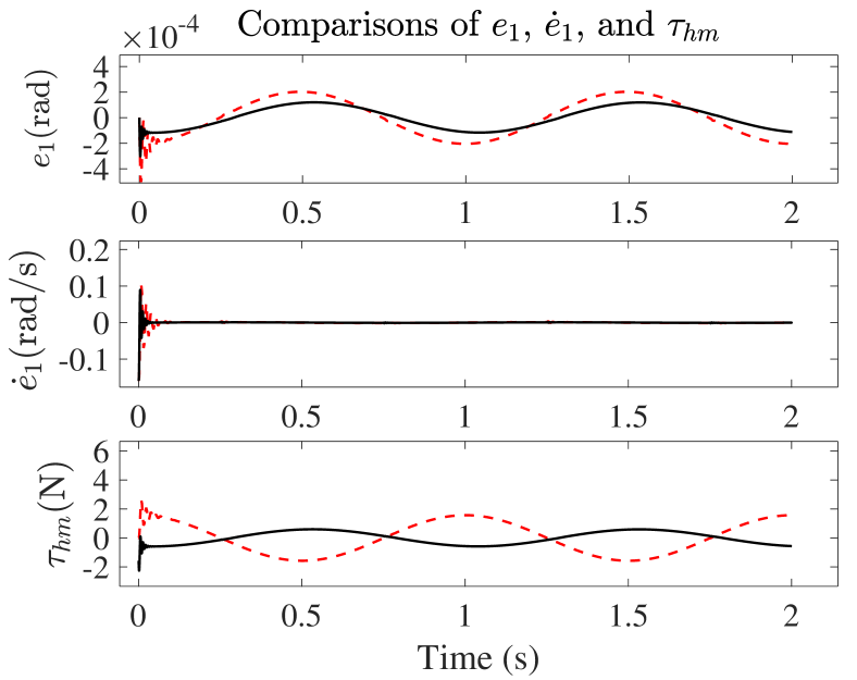
Figure 6: Comparison of $e_{1}$, $\dot{e}_{1}$, and $\tau_{hm}$: black solid lines represent the values computed with the proposed approach, while red dashed lines stand for the ones computed with PD controller.

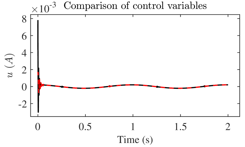
Figure 7: Comparison of control variable: black solid line is the values computed with the proposed approach, while red dashed line represent the one computed with PD controller..

In this section, simulation results are reported to show the performance of the hierarchical adaptive control algorithms previously described. The values of the key parameters of system (21) are listed in Table 1.

Table 1: Model parameters

Parameters	Values	Parameters	Values
$m$ ($kg$)	70	$C_{in}+C_{ex}$ ($m^{3}/s\cdot Pa$)	$2\times 10^{-14}$
$P_{p}$ ($MPa$)	5	$k_{s}$ (m/A)	0.0146
$b$ ($N\cdot s/m$)	5000	$A_{1}$ ($m^{2}$)	$3.25\times 10^{-4}$
$F_{C}$ ($N$)	8	$A_{2}$ ($m^{2}$)	$2.10^{-4}$
$\tau$ ($N\cdot s/m$)	0.0015	$l_{0}($m$)$	0.28
$K_{c}$ ($m^{3}s/Pa$)	$8.8\times 10^{-16}$	$K_{q}$ ($m^{3}s\cdot A$)	0.52
$x_{c0}(m)$	0.07	$l_{0}$ ($m$)	0.1

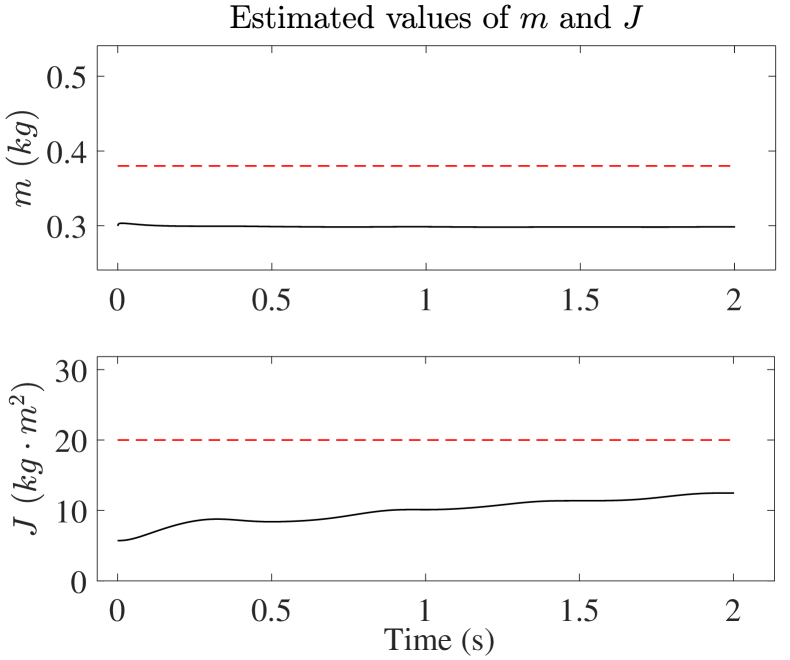
Figure 8: Estimated values of $m$ and $J$: black solid lines are the estimated values, while red dashed lines are the true ones.

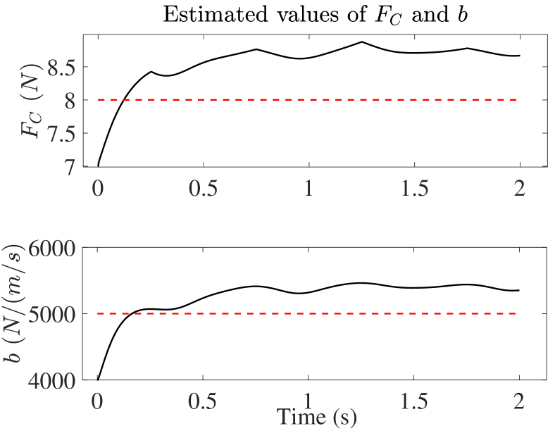
Figure 9: Estimated values of $F_{c}$ and $b$: black solid lines represent the estimated values, while red dashed lines stand for the true ones.

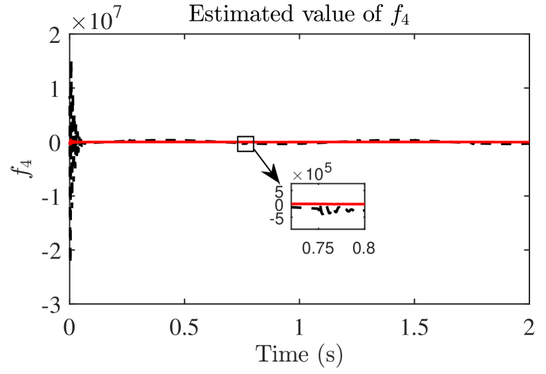
Figure 10: Estimated values of $f_{4}$: black solid lines is the estimated value, while red dashed line is the true one.

In the simulation experiment, the value of the reference joint angle has been set to $\phi_{d}=0.025sin(2\pi t)$ and the sampling time has been selected as $0.001$ $s$. The maximal value of the control variable is $u_{max}=2.5\times 10^{-2}$ $A$. The parameters in (13) are $k_{\varphi}=5000$ and $k_{\dot{\varphi}}=10$. The high-level regulator has been designed with $k_{1}=500$, $k_{2}=200$, and $\rho_{1}=\rho_{2}=1$. The corresponding adaptation algorithm has been devised with $q_{J}=1000$, $q_{m}=0.01$, $q_{1}=0.007$, and $q_{2}=0.0005$. The low-level controller has been implemented with $k_{3}=1000$, $\rho_{3}=1$. The parameter in (38) is selected as $\epsilon_{0}=0.001$, In neural network (45), the continuous RBF contains $n_{1}=3^{3}$ nodes with centers of $Z$ evenly spaced in the domain $[-4,\,4]\times[-1,\,1]\times[-4,\,4]$, and the values of the variance is chosen as $\upsilon=20000$. Also the nodes for the jump approximation function centered at $c_{1}$ and $c_{2}$ are $n_{2}=8\times 4$. The parameter for the updating law (47) is $\Gamma=100000I_{n_{1}+n_{2}+n_{3}}$ and the robust term is $\sigma=0.2I_{n_{1}+n_{2}+n_{3}}$. The simulation experiment has been run with null initial conditions. For comparison, a PD controller is designed with proportional gain $k_{P}=-1$ and derivative gain $k_{D}=-0.01$. The evolution of the states and control variables with the proposed approach and the PD algorithm, are reported in Figure. 6-7. From Figure. 6, it can be seen that after an initial transient, the proposed control algorithm shows satisfactory tracking performance, while the tracking error and the interaction torque computed with the proposed algorithm are smaller than that with the PD algorithm. Also, the estimations of the uncertain parameters and the nonlinear function $f_{4}$ of the system with the proposed algorithm are reported in Fig. 8-10, which shows that, the estimated values are close to their true values. Note that, some of the estimated values are not converging to their actual value. To further show the convergence properties of the estimated values, their true values must be known a-priori, which is usually nontrivial for practical reasons.

7 Conclusion

In this paper, a hierarchical Lyapunov-based adaptive cascade control scheme of a lower-limb exoskeleton with control saturation has been developed for joint angle position tracking objective. Adaptation algorithms have been proposed to estimate unknown model parameters at the both layers. At the lower layer, the neural network with continuous and discontinuous basis function has been used to approximate piecewise discontinuous nonlinear function. Thanks to the estimating techniques prescribed, the proposed approach allows to use imprecise models, which is much more reasonable for practical reasons. Moreover, with suitable control parameters design, this approach can also minimize the interaction torque between machine and human. The robustness of the closed-loop system has been discussed under control saturation. Simulation experiments including a comparison with PD have been reported, showing that the proposed approach is satisfactory in tracking performance and in interaction torque reduction, and outperforms PD controller in these respects. Future work will consider the use of learning based algorithms at the lower layer so as to optimize the switching condition between Mode1 and Mode2.

References

- [1] F. Abdollahi, H. A. Talebi, and R. V. Patel. A stable neural network-based observer with application to flexible-joint manipulators. IEEE Transactions on Neural Networks, 17(1):118–129, 2006.
- [2] N. Aliman, R. Ramli, and S. M. Haris. Design and development of lower limb exoskeletons: A survey. Robotics and Autonomous Systems, 95:102–116, 2017.
- [3] A. Alleyne and R. Liu. A simplified approach to force control for electro-hydraulic systems. Control Engineering Practice, 8(12):1347–1356, 2000.
- [4] K. Anam and A. Al-Jumaily. Active exoskeleton control systems: State of the art. Procedia Engineering, 2012.
- [5] A. Astolfi, D. Karagiannis, and R. Ortega. Nonlinear and adaptive control with applications. Springer Science & Business Media, 2007.
- [6] Robert Bogue. Robotic exoskeletons: a review of recent progress. Industrial Robot: An International Journal, 42(1):5–10, 2015.
- [7] H. Cao, J. Zhu, C. Xia, H. Zhou, X. Chen, and Y. Wang. Design and control of a hydraulic-actuated leg exoskeleton for load-carrying augmentation. In International Conference on Intelligent Robotics and Applications, pages 590–599. Springer, 2010.
- [8] S. Chantranuwathana and H. Peng. Adaptive robust force control for vehicle active suspensions. International Journal of Adaptive Control and Signal Processing, 18(2):83–102, 2004.
- [9] C. Chen. Backstepping control design and its applications to vehicle lateral control in automated highway systems. University of California at Berkeley, 1996.
- [10] M. Chen, S. S. Ge, and B. Ren. Adaptive tracking control of uncertain MIMO nonlinear systems with input constraints. Automatica, 47(3):452–465, 2011.
- [11] S. Chen, Z. Chen, B. Yao, X. Zhu, S. Zhu, Q. Wang, and Y. Song. Cascade force control of lower limb hydraulic exoskeleton for human performance augmentation. In Industrial Electronics Society, IECON 2016-42nd Annual Conference of the IEEE, pages 512–517. IEEE, 2016.
- [12] Mario di Bernardo, Umberto Montanaro, Romeo Ortega, and Stefania Santini. Extended hybrid model reference adaptive control of piecewise affine systems. Nonlinear Analysis: Hybrid Systems, 21:11–21, 2016.
- [13] Mario di Bernardo, Umberto Montanaro, and Stefania Santini. Hybrid model reference adaptive control of piecewise affine systems.
- [14] Luca Dieci and Luciano Lopez. Sliding motion on discontinuity surfaces of high co-dimension. a construction for selecting a filippov vector field. Numerische Mathematik, 117(4):779–811, 2011.
- [15] S. S. Ge and C. Wang. Direct adaptive nn control of a class of nonlinear systems. IEEE Transactions on Neural Networks, 13(1):214–221, 2002.
- [16] W. He, Y. Dong, and C. Sun. Adaptive neural impedance control of a robotic manipulator with input saturation. IEEE Transactions on Systems, Man, and Cybernetics: Systems, 46(3):334–344, 2016.
- [17] J. Huang, C. Wen, W. Wang, and Z. Jiang. Adaptive stabilization and tracking control of a nonholonomic mobile robot with input saturation and disturbance. Systems & Control Letters, 62(3):234–241, 2013.
- [18] R. Jimenez-Fabian and O. Verlinden. Review of control algorithms for robotic ankle systems in lower-limb orthoses, prostheses, and exoskeletons. Medical engineering & physics, 34(4):397–408, 2012.
- [19] H. Kazerooni, J. Racine, L. Huang, and R. Steger. On the control of the berkeley lower extremity exoskeleton (bleex). In Robotics and Automation, 2005. ICRA 2005. Proceedings of the 2005 IEEE international conference on, pages 4353–4360. IEEE, 2005.
- [20] H. Kim, Y.J. Shin, and J. Kim. Design and locomotion control of a hydraulic lower extremity exoskeleton for mobility augmentation. Mechatronics, 46:32–45, 2017.
- [21] Joseph LaSalle. Some extensions of liapunov’s second method. IRE Transactions on circuit theory, 7(4):520–527, 1960.
- [22] Z. Li, W. Ma, Z. Yin, and H. Guo. Tracking control of time-varying knee exoskeleton disturbed by interaction torque. ISA transactions, 71:458–466, 2017.
- [23] B. Llanas, S. Lantarón, and F. J. Sáinz. Constructive approximation of discontinuous functions by neural networks. Neural Processing Letters, 27(3):209–226, 2008.
- [24] M.J. Nandor. DESIGN AND FABRICATION OF AN ADVANCED EXOSKELETON FOR GAIT RESTORATION. PhD thesis, Case Western Reserve University, 2012.
- [25] Y Orlov, L Aguilar, and JC Cadiou. Switched chattering control of electrical servo-motors and backlash/friction attenuation. In Physics and Control, 2003. Proceedings. 2003 International Conference, volume 4, pages 1336–1341. IEEE, 2003.
- [26] X. Ouyang, S. Ding, B. Fan, P.Y. Li, and H. Yang. Development of a novel compact hydraulic power unit for the exoskeleton robot. Mechatronics, 38:68–75, 2016.
- [27] J. C. Racine. Control of a lower extremity exoskeleton for human performance amplification. 2003.
- [28] V. Santibañez, K. Camarillo, J. Moreno-Valenzuela, and R. Campa. A practical pid regulator with bounded torques for robot manipulators. International Journal of Control, Automation and Systems, 8(3):544–555, 2010.
- [29] Rastko Selmic and Frank L Lewis. Neural network approximation of piecewise continuous functions: application to friction compensation. In Intelligent Control, 1997. Proceedings of the 1997 IEEE International Symposium on, pages 227–232. IEEE, 1997.
- [30] Daniel Shevitz and Brad Paden. Lyapunov stability theory of nonsmooth systems. IEEE Transactions on automatic control, 39(9):1910–1914, 1994.
- [31] S. Song, X. Zhang, and Z. Tan. RBF neural network based sliding mode control of a lower limb exoskeleton suit. Strojniški vestnik-Journal of Mechanical Engineering, 60(6):437–446, 2014.
- [32] X. Wang, X. Li, J. Wang, X. Fang, and X. Zhu. Data-driven model-free adaptive sliding mode control for the multi degree-of-freedom robotic exoskeleton. Information Sciences, 327:246–257, 2016.
- [33] J. Xu, Y. Tan, and T. Lee. Iterative learning control design based on composite energy function with input saturation. Automatica, 40(8):1371–1377, 2004.
- [34] T. Yan, M. Cempini, C. M. Oddo, and N. Vitiello. Review of assistive strategies in powered lower-limb orthoses and exoskeletons. Robotics and Autonomous Systems, 64:120–136, 2015.
- [35] B. Yao, F. Bu, J. Reedy, and G. Chiu. Adaptive robust motion control of single-rod hydraulic actuators: theory and experiments. IEEE/ASME Transactions on Mechatronics, 5(1):79–91, 2000.
- [36] F. Zhao, S. S. Ge, F. Tu, Y. Qin, and M. Dong. Adaptive neural network control for active suspension system with actuator saturation. IET Control Theory & Applications, 10(14):1696–1705, 2016.
- [37] J. Zhou, M. J. Er, and J. M. Zurada. Adaptive neural network control of uncertain nonlinear systems with nonsmooth actuator nonlinearities. Neurocomputing, 70(4):1062–1070, 2007.
- [38] A. B. Zoss, H. Kazerooni, and A. Chu. Biomechanical design of the berkeley lower extremity exoskeleton (bleex). IEEE/ASME Transactions On Mechatronics, 11(2):128–138, 2006.