Solving the Grad-Shafranov equation using spectral elements for tokamak equilibrium with toroidal rotation
Abstract
The Grad-Shafranov equation is solved using spectral elements for tokamak equilibrium with toroidal rotation. The Grad-Shafranov solver builds upon and extends the NIMEQ code [Howell and Sovinec, Comput. Phys. Commun. 185 (2014) 1415] previously developed for static tokamak equilibria. Both geometric and algebraic convergence are achieved as the polynomial degree of the spectral-element basis increases. A new analytical solution to the Grad-Shafranov equation is obtained for Solov’ev equilibrium in presence of rigid toroidal rotation, in addition to a previously obtained analytical solution for a defferent set of equilibrium and rotation profiles. The numerical solutions from the extended NIMEQ are benchmarked with the analytical solutions, with good agreements. Besides, the extended NIMEQ code is benchmarked with the FLOW code [L. Guazzotto, R. Betti, et al., Phys. Plasma 11(2004)604].
keywords:
Magnetohydrodynamic equilibrium, Grad-Shafranov equation, NIMEQ, NIMROD, toroidal rotation, tokamak1 Introduction
For the static equilibrium, the magnetohydrodynamic (MHD) equations yield nonlinear second order differential equation known as Grad-Shafranov equation[1, 2]. The steady state equilibria defined by the solutions of Grad-Shafranov (GS)[1, 2] equation act as the foundation for evaluating the MHD stability of tokamak plasma. Numerical codes have been developed based on different algorithms to solve nonlinear GS equation for given plasma density, temperature and magnetic field profiles directly from experiment[3, 4]. However, most of these codes have only considered the static tokamak equilibrium where plasma flow such as the toroidal rotation is absent.
Toroidal rotation plays significant roles in many tokamak plasma processes. For example, plasma flow and flow shear above certain threshold may lead to the formations of H-mode and internal transport barrier (ITB)[5, 6, 7]. Meanwhile, plasma flow and flow shear can also directly affect plasma stability and transport[8, 9, 10, 11, 12, 13]. In particular, flow shear may have stabilizing effects on neoclassical tearing modes(NTMs)[14, 15], tearing modes (TMs)[16, 17, 18, 19] and edge localized modes(ELMs)[20, 12, 21, 22]. It is found that sufficient toroidal flow opens up a stability window for resistive wall mode (RWM)[23, 24, 25, 26, 11]. On the other hand, plasma flow and shear can also directly modify plasma equilibrium due to the centrifugal effect.
There is a rich history of analytic solution to the GS equation[27, 28, 29, 30, 31, 32, 33]. For example, the solution of the GS homogeneous equation is given by S. B. Zheng[27]. The inhomogeneous GS equation with linear source function and known as Solov′ev equilibrium can be solved analytically for any two parameters[27, 28]. The solution to the GS equation with parabolic source functions has been also reported, which allow independent specifications of plasma current density, pressure ratio and one shape moment such as the internal inductance[29, 30]. Besides tokamak, equilibria of other configurations also haved been obtained analytically, such as those of the field-reversed configuration (FRC)[31, 32].
However, the equilibriums that can be described using analytic solutions of GS equation are limited. GS equation often has to be solved numerically, based on the choice of either the flux along boundary or the source functions. Fixed-boundary solvers specify the flux value along the boundary of computation domain. Free-boundary solvers self-consistantly calculate the flux value along the boundary of computation, combining the contribution from external magnetic coils and the contribution from internal plasma current. Various numerical methods have been applied to solving the GS equation, for example, finite difference[34], spectral methods[35], Green’s functions[36], linear finite elements[37, 38], and Hermite cubic finite elements[39]. Consequently, many numerical toroidal equilibrium codes have been developed, such as EFIT[4], CHEASE[3], ESC[40], NIMEQ[41], etc.
In addition, several codes are able to solve for toroidal equilibrium in presence of flow, such as FLOW[8], CLIO[42] and FINESSE[43]. But these codes are often designed for topologically toroidal domains and do not consider the regularity issues associated with the singularity, where is the major radius. This issuse would arise in topologically cylindrical domains, which include the geometric axis .
Previously, a Grad-Shafranov solver NIMEQ[41] was developed for static toroidal equilibrium within the framework of NIMROD[44]. In this work, we extend the Grad-Shafranov solver NIMEQ[41] to solution of the toroidal equilibrium in presence of toroidal rotation. A new analytical solution of the modified Grad-Shafranov equation is found. The extended NIMEQ is benchmarked with the new analytical solution and the analytical solution by Maschke and Perrine[45]. The convergence of the extended NIMEQ is tested with h-refinement and p-refinement methods. Furthermore, the extended NIMEQ is benchmarked with FLOW in a convergence study.
The rest of this paper is organized as follows. Section (2) reviews the Grad-Shafranov equation with toroidal rotation. Section (3) shows a new analytical solution to the modified Grad-Shafranov equation along with the analytical solution obtained by Maschke and Perrin[45]. Section (4) presents the numerical algorithm of the extended NIMEQ. Benchmarking and convergence studies are performed with these two equilibria in section (5). Finally, section (6) gives conclusion and discussion.
2 Grad-Shafranov equation with toroidal rotation
Tokamak equilibria with toroidal rotation are governed by four equations: the force balance equation, magnetic divergence constraint, Ampere’s law and state equation of ideal gas[46]
| (1) | |||
| (2) | |||
| (3) | |||
| (4) |
where denotes the toroidal flow velocity, the frequency of toroidal rotation, the plasma pressure, the plasma current density, the magnetic field and the permeability of vacuum. Besides, denotes the mass density, defined as , and denotes the plasma temperature defined as , where (), () and are the ion (electron) mass, number density and temperature.
The magnetic field is expressed as and the plasma current is expressed as in the cylindrical coordinate system and is a flux function [41]. From the curl of Ohm’s law, it is observed that the frequency of toroidal rotation is a flux function . Substituting these above expressions for , and into Eq.(1) yields:
| (5) | |||
| (6) |
where the Grad-Shafranov operator is defined as
| (7) |
For fusion plasma the thermal conduction along magnetic field lines is fast compared to the heat transport perpendicular to a magnetic surface. Thus, plasma temperature can be considered as a flux function, namely . From Eq.(5), the pressure is integrated as:
| (8) |
Substituting into Eq.(6), we have
| (9) |
where denotes the position of magnetic axis. when . In the limit , the static equilibrium pressure can be recovered as a flux function. Meanwhile, Eq.(9) will reduce to the static GS equation.
3 Analytical solutions
3.1 Solov’ev equilibrium with toroidal rotation
We obtain a new analytical solution to Eq.(9) for Solov’ev equilibrium in presence of toroidal rotation. In Solov’ev equilibrium, we assume that:
| (10) | |||
| (11) |
where and are constants[47]. Furthermore, the plasma temperature and frequency of toroidal rotation are assumed to be constants and respectively, i.e. ,
The Grad-Shafranov equation Eq.(9) is reduced to
| (12) |
where denotes the Mach number at .
The solution of Eq.(12) is of the form , where is the particular solution and is the homogeneous solution[47, 27].
| (13) |
where these constants are determined by boundary condition. Then, for a particular solution:
| (14) |
We obtain a new analytical solution of Grad-shafranov equation for the Solov’ev equilibrium with toroidal rotation:
| (15) | |||
This solution reduces to the solution of static Solov’ev equilibrium when or .
3.2 Maschke-Perrin Equilibrium
| (18) | |||
| (19) | |||
| (20) |
where is the ratio of specific heats and , , , are constants.
In case of , the analytical solution takes the form
where is a constant, is a constant related to the ellipticity of the plasma cross-section, denotes the ratio between the position of magnetic axis and the chosen scale length .
4 Numerical algorithm
NIMEQ solves the Grad-Shafranov equation in weak form using Galerkin formulation[41]. Defining one scalar field , the Grad-Shafranov operator can be transformed into a divergence of a vector, . The scalar field can be spilt into two parts: and where satisfies the specified inhomogeneous boundary condition for and satisfies the boundary condition . The is expended onto a series of spectral element basis functions .The weak form of Grad-Shafranov equation is obtained as:
| (22) |
For compactness, Eq.(22) is written as . The modified Picard iterations in Eq.(23), has been applied to solve the Grad-Shafranov equation in NIMEQ, where denotes the relaxation parameter to achieve convergence.
| (23) |
After iteration, these equilibrium fields are calculated from the converged solution for . The pressure, temperature, toroidal flow velocity and values are calculated from the prescribed , , , using the converged solution through Eq.(8) and . The poloidal magnetic field is expressed as Eq.(24) in terms of .
| (24) |
where and represent the unit vectors in the and directions respectively.
The poloidal current is calculated directly from the magnetic field through the relation . And the toroidal current density is calculated using Eq.(25)
| (25) |
5 Benchmark and Convergence
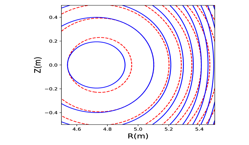
The analytic solutions in section 3.1 are plotted in a domain of rectangular poloidal cross section with and (Fig.1). Parameters are set as , , and the poloidal flux along the boundary is prescribed using Eq.(15), with , , and . The equilibrium poloidal flux contours for Solov’ev equilibrium with toroidal rotation and without toroidal rotation presented in Fig.1 show modification induced by toroidal rotation.
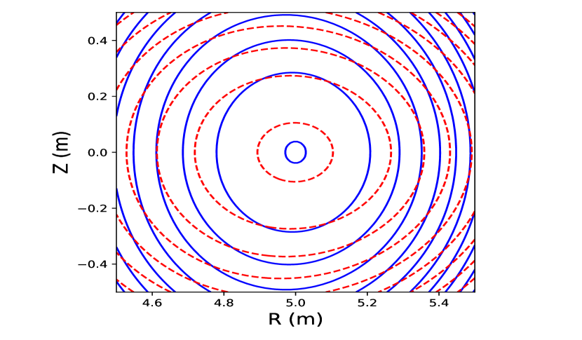
Similarly, the equilibrium poloidal flux contours for Maschke and Perrin’s equilibrium in section 3.2 are plotted in a domain of rectangular poloidal cross section with and (Fig.2). In this case, we choose , , , , , and . Distortion of flux surfaces due to toroidal rotation is also apparent.
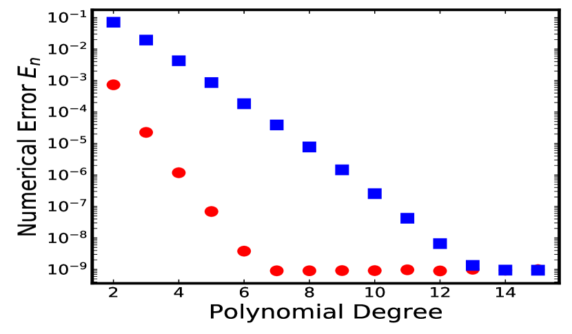
Both benchmark and convergence studies are performed for Solov’ev equilibrium and Maschke and Perrin’s equilibrium by comparing the numerical and analytical solutions. The numerical error of equilibrium poloidal flux is defined as , where is the numerical solution from the extended NIMEQ and is the analytic solution from Eq.(15) and Eq.(3.2). And the summation is performed over all of the finite-element nodes.
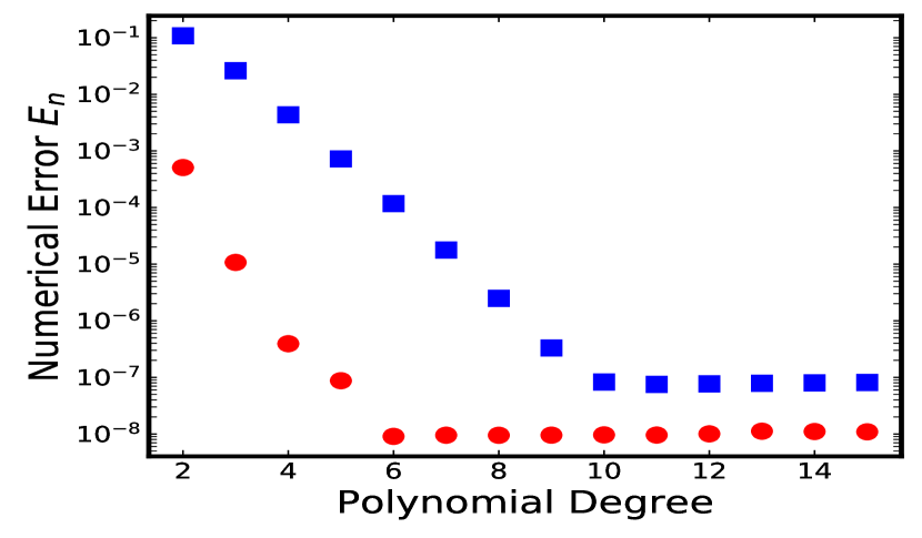
Two methods, i.e. h-refinement and p-refinement, are applied to checking the convergence of the extended NIMEQ in both equilibria. In the p-refinement method, the polynomial degree of each element is increased whereas the number of elements is kept constant. H-refinement maintains the polynomial degree of the elements while increasing the number of elements. The decaying rate of the error for a smooth solution of a second order differential equation is bounded by the asymptotic rate of convergence for sufficiently smooth solutions, where is a characteristic element length of calculation region and p is the polynomial degree[49].
We use meshes with equal numbers of elements in the radial and vertical directions. In the p-refinement study, the polynomial degree of elements is scanned from 2 to 15 when keeping the and element meshes fixed for both equilibria. In both equilibrium cases, the numerical errors decay linearly to a minimum value, which indicates geometric convergence in Fig.3 and Fig.5 [49]. The numerical error in element meshes decays faster than that in element meshes in both equilibria.
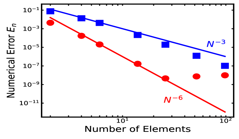
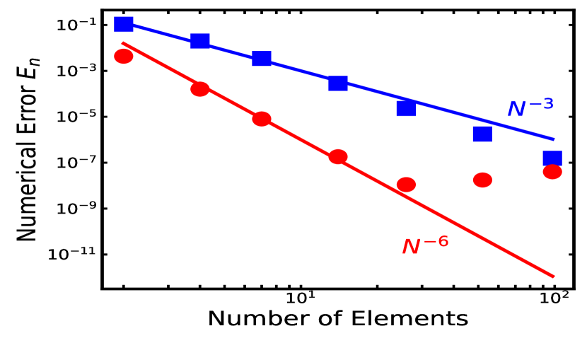
In h-refinement study, the number of elements are scanned from 4 to 94 when polynomial degree of elements keeps 2 and 4. In h-refinement studies of both equilibrium cases, the numerical errors decay linearly to a minimum value, indicating algebraic convergence in Fig.4 and Fig.6[49]. The decay rate of numerical erros with polynomial degree fixed 4 is larger than that with polynomial degree fixed 2. The blue lines in both figures stand for the scaling and fitted from the decaying numerical errors, where denotes the number of elements. Both figures show that the decay rates of numerical error in are between and .
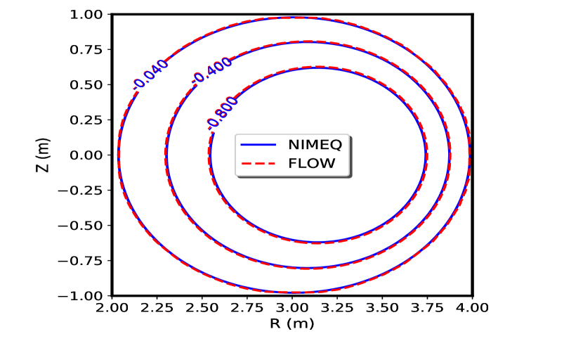
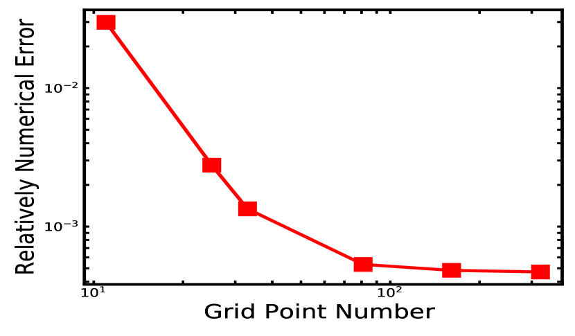
FLOW is a finite difference code, which solves the Bernoulli-Grad-Shafranov equations for tokamak the equilibriums with flow[8]. The extended NIMEQ is benchmarked with the FLOW code here. The comparison is performed in a poloidal domain of and . The and are chosen as constants. And the pressure profile is specified as one quadratic function of the normalized , . The number density profile is similar to the pressure profile, since , where and denote the pressure and number density on magnetic axis. This number density profile is thus chosen so as to obatain a consatnt temperature. The Mach number is constant and equals 0.3. The overlay of form the extended NIMEQ and FLOW is shown in Fig.7. For comparison, the relatively numerical error is defined as where denotes the numerical solution from NIMEQ and denotes the numerical solution from FLOW. Because the computation grids are different in NIMEQ and FLOW, the bi-cubic spline interpolation is applied to calculation of relatively numerical error. The relative numerical error decreases with the computation grid point number (Fig.8).
6 Conclusion and discussion
We have extended NIMEQ by solving the modified Grad-Shafranov equation that self-consistently takes into account of the effects of toroidal rotation. A new analytic solution to the modified Grad-Shafranov equation is obtained for the Solov’ev equilibrium in presence of a rigid toroidal rotation. Both the new analytical solution and the Maschke-Perrin equilibrium are used in benchmark and convergence studies. High accuracy solution with numerical error to the order of or smaller is achieved. The extended NIMEQ is also successfully benchmarked with the FLOW code.
Next we plan to extend the modified Grad-Shafranov equation to include free boundary condition, and to study the effects on equilibrium profiles due to toroidal rotation. Meanwhile, the poloidal flow can be also included in the extended NIMEQ to calculate equilibrium in presence of arbitrary flows.
Acknowledgments
This work was supported by the Fundamental Research Funds for the Central Universities at Huazhong University of Science and Technology Grant No. 2019kfyXJJS193, the National Natural Science Foundation of China Grant No. 11775221, the National Magnetic Confinement Fusion Science Program of China Grant No. 2015GB101004, and U.S. Department of Energy Grant Nos. DE-FG02-86ER53218 and DE-SC0018001. This research used the computing resources from the Supercomputing Center of University of Science and Technology of China.
References
- Grad and Rubin [1958] H. Grad, H. Rubin, Hydromagnetic equilibria and force-free fields, Journal of Nuclear Energy (1954) 7 (1958) 284–285.
- Shafranov [1958] V. Shafranov, On magnetohydrodynamical equilibrium configurations, Soviet Physics JETP 6 (1958) 1013.
- Lütjens et al. [1996] H. Lütjens, A. Bondeson, O. Sauter, The CHEASE code for toroidal MHD equilibria, Computer physics communications 97 (1996) 219–260. 00000.
- Lao et al. [2005] L. L. Lao, H. E. S. John, Q. Peng, J. R. Ferron, E. J. Strait, T. S. Taylor, W. H. Meyer, C. Zhang, K. I. You, MHD equilibrium reconstruction in the DIII-D tokamak, Fusion Science and Technology 48 (2005) 968–977.
- Ding et al. [2017] S. Ding, A. M. Garofalo, J. Qian, L. Cui, J. T. McClenaghan, C. Pan, J. Chen, X. Zhai, G. McKee, Q. Ren, X. Gong, C. T. Holcomb, W. Guo, L. Lao, J. Ferron, A. Hyatt, G. Staebler, W. Solomon, H. Du, Q. Zang, J. Huang, B. Wan, Confinement improvement in the high poloidal beta regime on DIII-D and application to steady-state H-mode on EAST, Physics of Plasmas 24 (2017) 056114.
- Sakamoto et al. [2001] Y. Sakamoto, Y. Kamada, S. Ide, T. Fujita, H. Shirai, T. Takizuka, Y. Koide, T. Fukuda, T. Oikawa, T. Suzuki, K. Shinohara, R. Yoshino, JT-60 Team, Characteristics of internal transport barriers in JT-60U reversed shear plasmas, Nuclear Fusion 41 (2001) 865–872.
- de Vries et al. [2009] P. de Vries, E. Joffrin, M. Brix, C. Challis, K. Crombé, B. Esposito, N. Hawkes, C. Giroud, J. Hobirk, J. Lönnroth, P. Mantica, D. Strintzi, T. Tala, I. Voitsekhovitch, Internal transport barrier dynamics with plasma rotation in JET, Nuclear Fusion 49 (2009) 075007.
- Guazzotto et al. [2004] L. Guazzotto, R. Betti, J. Manickam, S. Kaye, Numerical study of tokamak equilibria with arbitrary flow, Physics of Plasmas 11 (2004) 604–614.
- Shi et al. [2011] Y. Shi, G. Xu, F. Wang, M. Wang, J. Fu, Y. Li, W. Zhang, W. Zhang, J. Chang, B. Lv, J. Qian, J. Shan, F. Liu, S. Ding, B. Wan, S.-G. Lee, M. Bitter, K. Hill, Observation of cocurrent toroidal rotation in the east tokamak with lower-hybrid current drive, Phys. Rev. Lett. 106 (2011) 235001.
- Hegna [2016] C. C. Hegna, The effect of sheared toroidal rotation on pressure driven magnetic islands in toroidal plasmas, Physics of Plasmas 23 (2016) 052514.
- Wang and Ma [2015] S. Wang, Z. W. Ma, Influence of toroidal rotation on resistive tearing modes in tokamaks, Physics of Plasmas 22 (2015) 122504.
- Aiba et al. [2009] N. Aiba, S. Tokuda, M. Furukawa, P. Snyder, M. Chu, MINERVA: Ideal MHD stability code for toroidally rotating tokamak plasmas, Computer Physics Communications 180 (2009) 1282 – 1304.
- Yan et al. [2017] X. Yan, P. Zhu, Y. Sun, Neoclassical toroidal viscosity torque in tokamak edge pedestal induced by external resonant magnetic perturbation, Physics of Plasmas 24 (2017) 082510.
- Haye and Buttery [2009] R. J. L. Haye, R. J. Buttery, The stabilizing effect of flow shear on m/n=3/2 magnetic island width in DIII-D, Physics of Plasmas 16 (2009) 022107.
- Buttery et al. [2008] R. J. Buttery, R. J. L. Haye, P. Gohil, G. L. Jackson, H. Reimerdes, E. J. Strait, the DIII-D Team, The influence of rotation on the threshold for the 2∕1 neoclassical tearing mode in DIII-D, Physics of Plasmas 15 (2008) 056115.
- Wessen and Persson [1991] K. P. Wessen, M. Persson, Tearing-mode stability in a cylindrical plasma with equilibrium flows, Journal of Plasma Physics 45 (1991) 267–283.
- Haye et al. [2011] R. L. Haye, C. Petty, P. Politzer, the DIII-D Team, Influence of plasma flow shear on tearing in DIII-D hybrids, Nuclear Fusion 51 (2011) 053013.
- Sen et al. [2013] A. Sen, D. Chandra, P. Kaw, Tearing mode stability in a toroidally flowing plasma, Nuclear Fusion 53 (2013) 053006.
- Haye et al. [2010] R. J. L. Haye, D. P. Brennan, R. J. Buttery, S. P. Gerhardt, Islands in the stream: The effect of plasma flow on tearing stability, Physics of Plasmas 17 (2010) 056110.
- Cheng et al. [2017] S. Cheng, P. Zhu, D. Banerjee, Enhanced toroidal flow stabilization of edge localized modes with increased plasma density, Physics of Plasmas 24 (2017) 092510.
- Xia et al. [2013] T. Xia, X. Xu, P. Xi, Six-field two-fluid simulations of peeling-ballooning modes using BOUT++, Nuclear Fusion 53 (2013) 073009.
- Fenstermacher et al. [2013] M. Fenstermacher, X. Xu, I. Joseph, M. Lanctot, C. Lasnier, W. Meyer, B. Tobias, L. Zeng, A. Leonard, T. Osborne, Fast pedestal, SOL and divertor measurements from DIII-D to validate BOUT++ nonlinear ELM simulations, Journal of Nuclear Materials 438 (2013) S346 – S350. Proceedings of the 20th International Conference on Plasma-Surface Interactions in Controlled Fusion Devices.
- Chu et al. [1995] M. S. Chu, J. M. Greene, T. H. Jensen, R. L. Miller, A. Bondeson, R. W. Johnson, M. E. Mauel, Effect of toroidal plasma flow and flow shear on global magnetohydrodynamic MHD modes, Physics of Plasmas 2 (1995) 2236–2241.
- Ward and Bondeson [1995] D. J. Ward, A. Bondeson, Stabilization of ideal modes by resistive walls in tokamaks with plasma rotation and its effect on the beta limit, Physics of Plasmas 2 (1995) 1570–1580.
- Gerhardt et al. [2009] S. Gerhardt, D. Brennan, R. Buttery, R. L. Haye, S. Sabbagh, E. Strait, M. Bell, R. Bell, E. Fredrickson, D. Gates, B. LeBlanc, J. Menard, D. Stutman, K. Tritz, H. Yuh, Relationship between onset thresholds, trigger types and rotation shear for the m/n = 2/1 neoclassical tearing mode in a high-β spherical torus, Nuclear Fusion 49 (2009) 032003.
- Betti [1998] R. Betti, Beta limits for the n=1 mode in rotating-toroidal-resistive plasmas surrounded by a resistive wall, Physics of Plasmas 5 (1998) 3615–3631.
- Zheng et al. [1996] S. B. Zheng, A. J. Wootton, E. R. Solano, Analytical tokamak equilibrium for shaped plasmas, Physics of Plasmas 3 (1996) 1176–1178.
- Atanasiu et al. [2004] C. Atanasiu, S. Günter, K. Lackner, I. Miron, Analytical solutions to the Grad-Shafranov equation, Physics of Plasmas 11 (2004) 3510–3518.
- Mc Carthy [1999] P. J. Mc Carthy, Analytical solutions to the Grad-Shafranov equation for tokamak equilibrium with dissimilar source functions, Physics of Plasmas 6 (1999) 3554–3560.
- Šesnić et al. [2014] S. Šesnić, D. Poljak, E. Slišković, A review of some analytical solutions to the Grad-Shafranov equation, in: 2014 22nd International Conference on Software, Telecommunications and Computer Networks (SoftCOM), IEEE, 2014, pp. 24–27.
- Parks and Schaffer [2003] P. Parks, M. Schaffer, Analytical equilibrium and interchange stability of single-and double-axis field-reversed configurations inside a cylindrical cavity, Physics of Plasmas 10 (2003) 1411–1423.
- Berk et al. [1981] H. L. Berk, J. H. Hammer, H. Weitzner, Analytic field-reversed equilibria, Physics of Fluids 24 (1981) 1758–1759.
- Wang [2004] S. Wang, Theory of tokamak equilibria with central current density reversal, Phys. Rev. Lett. 93 (2004) 155007.
- Johnson et al. [1979] J. Johnson, H. Dalhed, J. Greene, R. Grimm, Y. Hsieh, S. Jardin, J. Manickam, M. Okabayashi, R. Storer, A. Todd, D. Voss, K. Weimer, Numerical determination of axisymmetric toroidal magnetohydrodynamic equilibria, Journal of Computational Physics 32 (1979) 212 – 234.
- Ling and Jardin [1985] K. Ling, S. Jardin, The princeton spectral equilibrium code: PSEC, Journal of Computational Physics 58 (1985) 300 – 335.
- Lao et al. [1985] L. Lao, H. S. John, R. Stambaugh, A. Kellman, W. Pfeiffer, Reconstruction of current profile parameters and plasma shapes in tokamaks, Nuclear Fusion 25 (1985) 1611–1622.
- Blum et al. [1981] J. Blum, J. L. Foll, B. Thooris, The self-consistent equilibrium and diffusion code sced, Computer Physics Communications 24 (1981) 235 – 254.
- Gruber et al. [1987] R. Gruber, R. Iacono, F. Troyon, Computation of MHD equilibria by a quasi-inverse finite hybrid element approach, Journal of Computational Physics 73 (1987) 168 – 182.
- Lütjens et al. [1992] H. Lütjens, A. Bondeson, A. Roy, Axisymmetric MHD equilibrium solver with bicubic Hermite elements, Computer Physics Communications 69 (1992) 287 – 298.
- Zakharov and Pletzer [1999] L. E. Zakharov, A. Pletzer, Theory of perturbed equilibria for solving the Grad-Shafranov equation, Physics of Plasmas 6 (1999) 4693–4704.
- Howell and Sovinec [2014] E. Howell, C. Sovinec, Solving the Grad-Shafranov equation with spectral elements, Computer Physics Communications 185 (2014) 1415 – 1421.
- Semenzato et al. [1984] S. Semenzato, R. Gruber, H. Zehrfeld, Computation of symmetric ideal MHD flow equilibria, Computer Physics Reports 1 (1984) 389 – 425.
- Beliën et al. [2002] A. Beliën, M. Botchev, J. Goedbloed, B. van der Holst, R. Keppens, FINESSE: Axisymmetric MHD equilibria with flow, Journal of Computational Physics 182 (2002) 91 – 117.
- Sovinec et al. [2004] C. Sovinec, A. Glasser, T. Gianakon, D. Barnes, R. Nebel, S. Kruger, D. Schnack, S. Plimpton, A. Tarditi, M. Chu, Nonlinear magnetohydrodynamics simulation using high-order finite elements, Journal of Computational Physics 195 (2004) 355 – 386.
- Maschke and Perrin [1980] E. K. Maschke, H. Perrin, Exact solutions of the stationary MHD equations for a rotating toroidal plasma, Plasma Physics 22 (1980) 579.
- Masaru et al. [2000] F. Masaru, A. Yuji, A. Satoshi, W. Masahiro, Tokamak equilibria with toroidal flows, Journal of Plasma and Fusion Research 76 (2000) 937–948.
- Solov’ev [1968] L. Solov’ev, The theory of hydromagnetic stability of toroidal plasma configurations, Sov. Phys. JETP 26 (1968).
- Chu et al. [2018] M. S. Chu, Y. Hu, W. Guo, Generalization of Solovev’s approach to finding equilibrium solutions for axisymmetric plasmas with flow, Plasma Science and Technology 20 (2018) 035101.
- Boyd [2000] J. P. Boyd, Chebyshev and Fourier Spectral Methods, Second Edition ed., DOVER Publications, Inc., 2000.