The Hi Velocity Function: a test of cosmology or baryon physics?

Abstract

Accurately predicting the shape of the Hi velocity function of galaxies is regarded widely as a fundamental test of any viable dark matter model. Straightforward analyses of cosmological $N$-body simulations imply that the $\Lambda$CDM model predicts an overabundance of low circular velocity galaxies when compared to observed Hi velocity functions. More nuanced analyses that account for the relationship between galaxies and their host haloes suggest that how we model the influence of baryonic processes has a significant impact on Hi velocity function predictions. We explore this in detail by modelling Hi emission lines of galaxies in the Shark semi-analytic galaxy formation model, built on the surfs suite of $\Lambda$CDM $N$-body simulations. We create a simulated ALFALFA survey, in which we apply the survey selection function and account for effects such as beam confusion, and compare simulated and observed Hi velocity width distributions, finding differences of $\lesssim 50$%, orders of magnitude smaller than the discrepancies reported in the past. This is a direct consequence of our careful treatment of survey selection effects and, importantly, how we model the relationship between galaxy and halo circular velocity - the Hi mass-maximum circular velocity relation of galaxies is characterised by a large scatter. These biases are complex enough that building a velocity function from the observed Hi line widths cannot be done reliably.

1 Introduction

The $\Lambda$ Cold Dark Matter (hereafter $\Lambda$CDM) model is well established as the Standard Cosmological Model, naturally predicting the structure of the Universe on intermediate-to-large scales and explaining a swathe of observational data, from the formation and evolution of large scale structure, to the state of the Early Universe, to the cosmic abundance of different types of matter (e.g. Bull et al. 2016).

Despite its numerous successes, however, the $\Lambda$CDM model faces a number of challenges on small scales. Cold dark matter (hereafter CDM) haloes form cuspy profiles (i.e. the dark matter density rises steeply at small radii Navarro et al., 1995), whereas observational inferences suggest that low mass dark matter (hereafter DM) dominated galaxies have constant-density DM cores (Duffy et al., 2010; Oman et al., 2015; Dutton et al., 2018), leading to the so-called “cusp-core" problem. CDM haloes are also predicted to host thousands of subhaloes, which has led to the conclusion that the Milky Way suffers from a “missing satellites” problem because it should host many more satellite galaxies than the $\sim 50$ that are observed (Bullock & Boylan-Kolchin, 2017). While the inefficiency of galaxy formation in low-mass haloes - because of feedback processes such as e.g. cosmological reionization, supernovae, etc… - may lead to many subhaloes to be free of baryons and dark, the “too big to fail” problem (Boylan-Kolchin et al., 2011) suggests that the central density of CDM subhaloes are too high; in dissipationless $\Lambda$CDM simulations of Milky Way mass haloes, the most massive subhaloes, which are large enough to host galaxy formation and so “too big to fail”, have typical circular velocities  1.5 times higher ($\sim 30$  km s^-1) than that observed at the half-light radii of the Milky Way satellite. This indicates that there are problems with both the predicted abundances and internal structures of CDM subhaloes (Dutton et al., 2016).

Interestingly, with the emergence of observational surveys sensitive enough to detect statistical samples of faint galaxies in the nearby Universe, it has become clear that there is a consistent deficit in the observed abundance of low mass galaxies when compared to predictions from the $\Lambda$CDM model (e.g. Tollerud et al., 2008; Hargis et al., 2014). This suggests that the “missing satellite” problem is more generically a “missing dwarf galaxy” problem. This is most evident in measurements of the velocity function (VF) - the abundance of galaxies as a function of their circular velocity. The observed VF is assumed to be equivalent to the VF of DM subhaloes (Gonzalez et al., 2000), and so its measurement should provide a potentially powerful test of the Standard Cosmological Model.

The utility of the VF as a test of DM is already evident in the results of the Hi VF measured by ALFALFA (The Arecibo Legacy Fast ALFA: Giovanelli et al., 2005); focusing on galaxies with rotational velocities of $\sim 25$  km s^-1, the ALFALFA VF found approximately an order of magnitude fewer galaxies than expected from cosmological CDM simulations (Klypin et al., 2014; Brooks et al., 2017). Trujillo-Gomez et al. (2018) attempted to correct the measured Hi velocities by including the effects of pressure support and derive a steeper VF, though still shallower than the $\Lambda$CDM prediction. This has prompted interest in Warm Dark Matter (hereafter WDM) models, which predict significantly less substructure within haloes (Macciò et al., 2012; Zavala et al., 2009). The linear matter power spectrum in WDM cosmologies is characterised by a steep cutoff at dwarf galaxy scales, which results in the suppression of low-mass structure formation and a reduction in the number of dwarf galaxies such that the VF predicted by the WDM model is more consistent with observations (Schneider et al., 2012). While the WDM model has the potential to provide a better description of the observed VF, there is a tension between the range of WDM particle masses required ($<$ 1.5 keV; cf. Schneider et al., 2017) and independent observational constraints from the Lyman-$\alpha$ forest at high redshifts, which rule out such low WDM particle masses (Klypin et al., 2014).

An alternative solution that has been recently discussed to alleviate the discrepancy between the observed and predicted VF is the effect of baryonic physics. Brooks et al. (2017) and Macciò et al. (2016) used cosmological zoom-in hydrodynamical simulations of a small number of galaxies (typically ranging from $30$ to $100$) to produce Hi emission lines for their galaxies. They measured $W_{50}$ (width of the Hi emission line at $50$% of the maximum peak flux), which is used as a proxy in observations to estimate the Hi velocity of the galaxy, and then compared them with the rotational velocity, $V_{\rm\textsc{dmo}}$, of the haloes from the dark matter only (DMO) simulations. They found that due to the effect of baryons, $W_{50}$ and $V_{\rm\textsc{dmo}}$ are non-linearly correlated, in a way that $W_{50}$ tends to underestimate $V_{\rm\textsc{dmo}}$ in low mass haloes, while the opposite happens at the high-mass end. They propose that a DM density profile that varies with stellar-to-halo mass ratio can be used to reconcile the differences with the observations. Trujillo-Gomez et al. (2018), however, showed that including the feedback-induced deviations from the $\Lambda$CDM VF predicted by the hydrodynamical simulations above were insufficient to reproduce the observed VF.

Although the work of Brooks et al. (2017) and Macciò et al. (2016) present a compelling solution to the apparent missing dwarf galaxy problem, their sample is statistically limited. Obreschkow et al. (2013) approached this problem from a different perspective, with much better statistics (going into a million of simulated galaxies). They attempted to see how the selection biases of the surveys might contribute to this problem. Their solution was to make a mock-survey using DMO $N$-body simulations combined with semi-analytic models of galaxy formation, and then compare its results with the actual observations via producing a lightcone (see $\S$ 2.1) with all the required selection effects. They did this for the HIPASS survey (Hi Parkes All-Sky Survey: Meyer et al., 2004), as their simulation was limited in resolution to moderate halo masses, and hence was more directly comparable to HIPASS. HIPASS is the first blind Hi survey in the Southern Hemisphere with a velocity range of $-1280$ to $12700$  km s^-1, identifying over $5317$ Hi sources in total (including both Northern and Southern Hemispheres). Obreschkow et al. (2013) found that the observed Hi linewidths were consistent with $\Lambda$CDM at the resolution of the Millennium simulation (Springel et al., 2005), though they could not comment on haloes of lower mass, in which the largest discrepancies have been reported.

The main limitations of the works above have been either statistics or limited resolution. Here, we approach this problem with the surfs suite (Elahi et al., 2018) of $N$-body simulations, which covers a very large dynamic range, from circular velocities of $20$  km s^-1 to $>500$  km s^-1, and combine it with the state-of-the-art semi-analytic model Shark (Lagos et al., 2018), which includes a sophisticated multi-phase interstellar medium modelling. We use these new simulations and model to build upon the work of Obreschkow et al. (2013), and present a thorough comparison with the $100\%$-data release of ALFALFA (Haynes et al., 2018). We focus on the ALFALFA survey as it is a blind Hi survey and covers a greater cosmological volume with a better velocity and spatial resolution than other previous Hi surveys. We show that our simulated ALFALFA lightcone produces a $W_{50}$ distribution in very good agreement with the observations, even down to the smallest galaxies detected by ALFALFA, and discuss the physics behind these results and their implications.

This paper is organised as follows. $\S$ 2 describes the galaxy formation model used in this study and the construction of the mock ALFALFA survey. In $\S$ 3, the modelling of the Hi emission lines is described along with its application on the mock-sky built in the previous section. $\S$ 4, we compare our results with ALFALFA observations and discuss our results in the context of previous work. $\S$ 5 summarises our main results. In the Appendix A we compare our model for the Hi emission line of galaxies with the more complex Hi emission lines obtained from the cosmological hydrodynamical simulations apostle (Oman et al., 2019).

2 The simulated galaxy catalogue

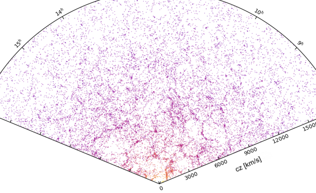
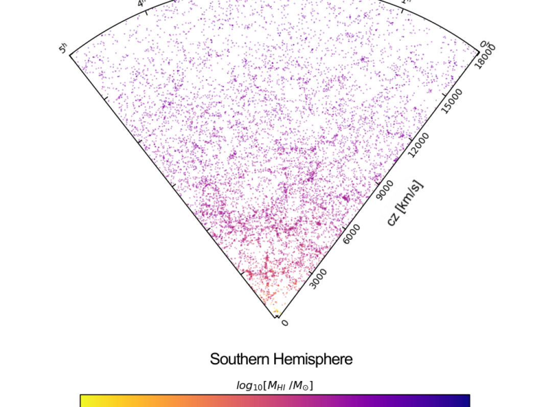
Figure 1: Mock sky of the ALFALFA survey, created with the outputs of Shark and processed with Stingray to create the observable sky. Symbols show individual galaxies and colours show their Hi mass, as labelled by the colour bar at the bottom. Low Hi mass galaxies are only detected in the very nearby universe.

Our simulated galaxy catalogue is constructed using the Shark semi-analytic model (Lagos et al., 2018) that was run on the surfs $N$-body simulations suite (Elahi et al., 2018). Here, we describe briefly Shark and surfs.

Hierarchical galaxy formation models, such as Shark, require three basic pieces of information about DM haloes : (i) the abundance of haloes of different masses; (ii) the formation history of each halo; and in some cases (iii) the internal structure of the halo including their radial density and their angular momentum (Baugh, 2006). These fundamental properties are now well established, thanks to the $N$-body simulations like surfs (used in this study).

The surfs suite consists of $N$-body simulations of differing volumes, from $40\,h^{-1}$ cMpc to $210\,h^{-1}$ cMpc on a side, and particle numbers, from $\sim\!130$ million up to $\sim\!8.5$ billion particles, using the $\Lambda$CDM Planck cosmology (Planck Collaboration XIII 2016). The latter has a total matter, baryon and dark energy densities of $\Omega_{\rm m}=0.3121$, $\Omega_{\rm b}=0.0491$ and $\Omega_{\rm L}=0.6751$, and a dimensionless Hubble parameter of $h=0.67512$. The surfs suite is able to resolve DM haloes down to $8.3\times 10^{8}\,h^{-1}$ $\rm{M}_{\odot}$. For this analysis, we use the L40N512 and L210N1536 runs, referred to as micro-surfs and medi-surfs  respectively hereafter, whose properties are given in Table 1. Merger trees and halo catalogues were constructed using the phase-space finder velociraptor (Elahi et al., 2019a; Welker et al., 2018) and the halo merger tree code TreeFrog (Poulton et al., 2018; Elahi et al., 2019b).

Shark was introduced by Lagos et al. (2018), and is an open source, flexible and highly modular cosmological semi-analytic model of galaxy formation, which is hosted in GitHub. It models key physical processes that shape the formation and evolution of galaxies, including (i) the collapse and merging of DM haloes; (ii) the accretion of gas onto haloes, which is governed by the DM accretion rate; (iii) the shock heating and radiative cooling of gas inside DM haloes, leading to the formation of galactic discs via conservation of specific angular momentum of the cooling gas; (iv) the formation of a multi-phase interstellar medium and star formation in galaxy discs; (v) the suppression of gas cooling due to photo-ionisation; (vi) chemical enrichment of stars and gas; (vii) stellar feedback from the evolving stellar populations; (viii) the growth of supermassive black holes via gas accretion and merging with other black holes; (ix) heating by active galactic nuclei (AGN); (x) galaxy mergers driven by dynamical friction within common DM haloes which can trigger bursts of star formation (SF) and the formation and/or growth of spheroids; and (xi) the collapse of globally unstable discs that also lead to the bursts of SF and the formation and/or growth of bulges. Shark includes several different models for gas cooling, AGN feedback, stellar and photo-ionisation feedback, and star formation. The model also numerically evolves the exchange of mass, metals and angular momentum between the key gas reservoirs of haloes and galaxies: halo hot and cold gas, galaxy stellar and gaseous’ disc and bulge (and within discs between the atomic and molecular gas), central black hole, and the ejected gas component (outside haloes).

Table 1: surfs simulation parameters of the runs being used in this paper. We refer to L40N512 and L210N1536 as micro-surfs and medi-surfs, respectively.

Name	Box size	Number of	Particle Mass	Softening Length
	$L_{\rm box}[\rm cMpc/h]$	Particles $N_{\rm p}$	$m_{\rm p}$ [$\rm{M}_{\odot}$/h]	$\epsilon[\rm ckpc/h]$
L40N512	$40$	$512^{3}$	$4.13\times 10^{7}$	2.6
L210N1536	$210$	$1536^{3}$	$2.21\times 10^{8}$	4.5

Halo gas in Shark is assumed to be in two phases: cold, which is expected to cool within the duration of a halo’s dynamical time; and hot, which remains at the virial temperature of the halo. Cold gas is assumed to settle onto the disc and follows an exponential profile of half-mass radius $r_{\rm gas,disc}$. In our model $r_{\rm gas,disc}$ can differ from the stellar half-mass radius as stars form only from the molecular hydrogen (H₂) and not the total gas. Surface densities of Hi and H₂ are calculated using the pressure relation of Blitz & Rosolowsky (2006), described in detail in $\S$ 3.1.

Models and parameters used in this study are the defaults of Shark as described in Lagos et al. (2018), which were calibrated to reproduce the $z=0,\,1,\,2$ stellar mass functions (SMFs); the $z=0$ black hole-bulge mass relation; and the disc and bulge mass-size relations. In addition, the model reproduces well observational results that are independent of those used in calibration, including the total neutral, atomic and molecular hydrogen-stellar mass scaling relations at $z=0$; the cosmic star formation rate (SFR) density evolution up to $z\approx 4$; the cosmic density evolution of the atomic and molecular hydrogen at $z\lesssim 2$ or higher in the case of the latter; the mass-metallicity relations for the gas and stars; the contribution to the stellar mass by bulges and the SFR-stellar mass relation in the local Universe. Davies et al. (2018) show that Shark also reproduces the scatter around the main sequence of star formation in the SFR-stellar mass plane, while Martindale et al. (in preparation) show that Shark reproduces the Hi content of groups as a function of halo mass. Of particular importance for this study is Shark’s success in recovering the observed gas abundances of galaxies.

2.1 A mock ALFALFA sky

To ensure a fair comparison with available Hi surveys, we first estimate how predicted galaxy properties are likely to be influenced by the choice of selection criterion. Here, mock galaxy catalogues are a particularly powerful tool, and so we begin by constructing a “mock ALFALFA" survey. We do this by generating a galaxy population with Shark and embed them within a cosmological volume by applying the survey’s angular and radial selection functions (e.g. Merson et al., 2013).

We use the code stingray, which is an extended version of the lightcone of Obreschkow et al. (2009c), to build our lightcones from the Shark outputs. Rather than forming a single chain of replicated simulation boxes, stingray tiles boxes together to build a more complex 3D field along the line-of-sight of the observer. Galaxies are drawn from simulation boxes which correspond to the closest look-back time, which ranges over the redshift range $z=0$ to $z=0.06$ (corresponding to the ALFALFA limit); in the Shark simulations, this corresponds to the last 7 snapshots. Properties of each galaxy in the lightcone are obtained from the closest available time-step, resulting in the formation of spherical shells of identical redshifts. A possible issue would be the same galaxy appearing once in every box, but due to cosmic evolution might display different intrinsic properties. In order to avoid this problem, galaxy positions are randomised by applying a series of operations consisting of $90$ deg-rotations, inversions, and continuous translations. We build the lightcones with all the galaxies in Shark that have a stellar or cold gas mass (atomic plus molecular) $\geq 10^{6}\,\rm M_{\odot}$. Any additional selection (in this case the one specific to ALFALFA) are applied later, directly to the lightcone galaxies. The end result of the whole process is that we get a mock-observable sky as shown in Figure 1 which is as near to the real sky as possible and with minimum repetition of the large-scale structure. The two portions of the sky shown correspond to the north and south ALFALFA regions.

stingray also computes an inclination for each galaxy with respect to the observer. The latter are constructed assuming galaxies to have an angular momentum vector of the same direction as of its subhalo angular momentum vector (as measured by velociraptor ), in the case of central galaxies and satellites galaxies type =1. For type=2 satellite galaxies we assume random orientations. Satellites type=1 correspond to those hosted by satellite subhalos that are identified by velociraptor, while satellites type=2 correspond to those that were hosted by subhalos that have ceased to be identified by velociraptor. The latter usually happens when subhalos become too low mass to be robustly identified (see Poulton et al. 2018 for a detailed analysis of satellite subhalo orbits). The overall effect of inclinations is to reduce $W_{50}$.

A limitation of any observational survey is finite velocity and spatial resolution, which for a survey like ALFALFA can lead to 2 or more galaxies falling inside the same beam and then overlapping in frequency, more commonly known as “beam confusion”. To mimic the effect of confusion in our analysis, we merge simulated galaxies whose centroids are separated by less than a projected 3.8’ (the full-width-half-max for the ALFALFA beam) and whose Hi lines overlap in frequency. In the case of galaxies being confused, the common Hi mass is taken as the sum of the individual Hi masses of the galaxies, and the $W_{50}$ (the full-width at half of the peak flux of the line)is measured for the combined line formed due to the overlapping Hi lines. Obreschkow et al. (2013) found that “confused" galaxies typically have high Hi-mass and $W_{50}$, with $M_{\rm HI}>10^{10}$$\rm{M}_{\odot}$ and $W_{50}>300$ km s^-1, albeit for the HIPASS survey, which has a larger beam than ALFALFA; we find fewer confused galaxies lying in this range in our sample. By including confusion, we reduce the total number of galaxies by $<1$%, throughout the whole dynamical range of galaxies.

To ensure that we have the dynamical range in circular velocity in our sample of galaxies required to test the “missing satellite problem”, we make two lightcones using the micro- and medi-surfs; micro-surfs gives us better mass resolution to probe down to dwarf galaxies, with $M_{\rm HI}\lesssim 10^{9}M_{\odot}$, while medi-surfs provides us with a much larger volume and better statistics at the high-mass end, $M_{\rm HI}\gtrsim 10^{9}M_{\odot}$. Results for these lightcones are presented in § 4.2.

3 Modelling Hi emission lines in Galaxy Formation Models

In this section, we describe the steps required to build an Hi emission line for each Shark galaxy. $\S$ 3.1 and $\S$ 3.2 provide details of the surface density and velocity profile calculations, respectively. The way we combine them to create the Hi emission line is described in $\S$ 3.3.

3.1 Gas mass and profile

For the calculation of the Hi surface density profile, we adopt the empirical model described in Blitz & Rosolowsky (2004, 2006) (Equation 1). In their model, the ratio of molecular to atomic hydrogen gas surface density in galaxies is a function of hydro-static pressure in the mid-plane of the disc, with a power-law index close to $1$,

$$R_{\rm mol}(r)=\left[P_{\rm ext}(r)/P_{\star}\right]^{\alpha},$$ (1)

where $R_{\rm mol}\equiv\Sigma_{\rm H_{2}}/\Sigma_{\rm HI}$, with $\Sigma_{\rm H_{2}}$ and $\Sigma_{\rm HI}$ being the surface density of molecular and atomic hydrogen, respectively. The parameters $P_{\star}$ and $\alpha$ are measured in observations, and in Shark we adopt $P_{\star}=34,673{\rm\,Kcm^{-3}}$ and $\alpha=0.92$, which correspond to the best fit values in Blitz & Rosolowsky (2006).

Blitz & Rosolowsky (2006) adopted the Elmegreen (1989) estimate of $P_{\rm ext}$ for disc galaxies, which corresponds to the mid-plane pressure in an infinite, two-fluid disc with locally isothermal stellar and gas layers,

$$P_{\rm ext}(r)=\frac{\pi}{2}G\Sigma_{\rm g}\left[\Sigma_{\rm g}+\left(\frac{\sigma_{\rm gas}}{\sigma_{\star}}\right)\Sigma_{\star}\right],$$ (2)

where $P_{\rm ext}(r)$ is the kinematic mid-plane pressure outside molecular clouds, and the input for Equation 1. $G$ is the gravitational constant, $\Sigma_{g}$ is the total gas surface density (atomic plus molecular), $\Sigma_{\star}$ is the stellar surface density, and $\sigma_{\rm gas}$ and $\sigma_{\star}$ are the gas and stellar vertical velocity dispersion, respectively.

The stellar and gas surface densities are assumed to follow exponential profiles with a half-gas and half-stellar mass radii of $r_{\rm gas,disc}$ and $r_{\star,\rm disc}$, respectively. We adopt $\sigma_{\rm gas}=10\,\rm km\,s^{-1}$ (Leroy et al., 2008) and calculate $\sigma_{\star}=\sqrt{\pi\,G\,h_{\star}\,\Sigma_{\star}}$. Here, $h_{\star}$ is the stellar scale height, and we adopt the observed relation $h_{\star}=r_{\rm\star,disc}/7.3$ (Kregel et al., 2002), with $r_{\rm\star,disc}$ being the half-stellar mass radius.

Figure 2 shows the radial surface density profile for an example galaxy in Shark  with a stellar and Hi mass of $10^{9}$ $\rm{M}_{\odot}$ and $10^{8}$ $\rm{M}_{\odot}$, respectively. The inner radius is dominated by H₂, with Hi forming a core there. The latter is due to the saturation of Hi at high column densities, above which the gas is converted into H₂. The sum of both gas components is exponential, however, the individual ones can deviate from that assumption. Hi typically dominates at the outer radius.

Previous work by Obreschkow et al. (2009a) and Obreschkow et al. (2013) assumed the total gas disc to have an exponential profile with a scale length that was larger than the stellar one by a factor $>1$. They determined the Hi/H₂ ratio locally in post-processing using the Blitz & Rosolowsky (2006) model, with updated empirical parameters obtained from THINGS (The HI Nearby Galaxy Survey Walter et al., 2008). Thus, our work improves on this by (i) allowing the Hi to have a more complex profile, such as the example of Figure 2, though still axisymmetric, and (ii) by calculating the multi-phase nature of galaxies self-consistently within the galaxy formation calculation. The latter directly impacts galaxy evolution as stars can only form from molecular hydrogen in Shark. In our model, Hi can also exist in the bulges of galaxies, which in general allows the models to reproduce the observed gas content of early-type galaxies (Lagos et al., 2014; Serra et al., 2010; Lagos et al., 2018).

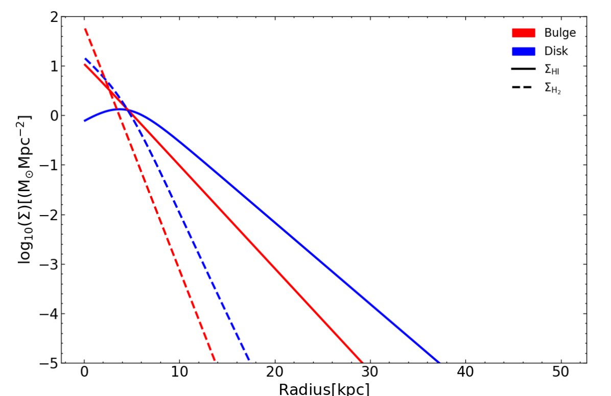
Figure 2: Surface density radial profiles of Hi in the disc and bulge, as labelled, for an example Shark galaxy, used to model the Hi emission lines. The solid and dashed lines represents the Hi and H₂ surface density of the galaxy, respectively. As it can be seen, there is a presence of Hi in the bulge of the galaxy, which drops down steeply in the beginning, but the Hi in the disc extends much further, and dominates beyond $\gtrsim 4$ kpc. There is a significant amount of H₂ present in the bulge, though it declines much more rapidly than the extended Hi disc.

3.2 Circular velocity profile

The circular velocity profiles are constructed following Obreschkow et al. (2009a), which we briefly describe in this section. We assume a Navarro-Frenk-White (NFW; Navarro et al., 1995) halo radial profile, which describes the DM halo density profiles not as isothermal (i.e. $\rho\propto r^{-2}$) but with a radially varying logarithmic slope

$$\rho_{\rm halo}(r)\ =\ \rho_{0}\left[(r/r_{\rm s})(1\ +\ r/r_{s})^{2}\right]^{-1},$$ (3)

where $\rho_{0}$ is a normalization factor and $r_{s}$ is the characteristic scale radius of the halo (where the profile has a logarithmic slope of $-2$). The virial radius, $r_{\rm vir}$  is calculated using the virial velocity of the haloes, $V_{\rm vir}$, following the relation,

$$r_{\rm vir}\ =\ \frac{GM_{\rm vir}}{V_{\rm vir}^{2}},$$ (4)

where $M_{\rm vir}$ is the virial mass of the halo. Here, we define the virial mass as the mass enclosed within the halo when the overdensity is $200$ times that of critical density. The scale radius, $r_{s}$, is defined as $r_{s}\ =\ r_{\rm vir}/c_{\rm halo}$, where $c_{\rm halo}$ is the concentration parameter, which in Shark is estimated using the Duffy et al. (2008) relation.

For a spherical halo, the circular velocity profile will be $V_{c}^{\rm halo^{2}}\ =\ \frac{GM_{\rm halo}(r)}{r}$, where $M_{\rm halo}(r)$ is the mass enclosed within the radius $r$. Therefore, the circular velocity profile of the halo is,

$$V_{c}^{\rm halo^{2}}(x)=\left(\frac{GM_{\rm vir}}{r_{\rm vir}}\right)\ \times\ \frac{{\rm ln}(1+c_{\rm halo}x)-\frac{c_{\rm halo}x}{1+c_{\rm halo}x}}{x\left[{\rm ln}(1+c_{\rm halo})-\frac{c_{\rm halo}}{1+c_{\rm halo}}\right]},$$ (5)

where $x\ \equiv\ r/r_{\rm vir}$. For larger radii, the circular halo velocity approaches the point mass velocity profile $V_{c}^{\rm halo^{2}}\ \approx\ GM_{\rm vir}/r$.

For the velocity profile of the disc, we use the stellar and gas surface densities calculated with SharkṠtellar and gas surface density profiles are assumed to follow an exponential form with a distinct half mass radius for stellar and gas components. We calculate velocity profiles for stars and gas separately and then combine them to give $V_{\rm c}^{\rm disc}$. Following Obreschkow et al. (2009a), we define the circular velocity for the stellar disc, $V_{\rm c}^{\rm\star,disc}$, as

$$\begin{multlined}V_{\rm c}^{\rm\star,disc^{2}}(x)\approx\frac{G\,M^{\rm\star,disc}}{r_{\rm vir}}\ \times\\ \frac{c_{\rm\star,disc}+4.8\,c_{\rm\star,disc}\,{\rm exp}[-0.35\,c_{\rm\star,disc}\,x-3.5/(c_{\rm\star,disc}\,x)]}{c_{\rm\star,disc}\,x+\left(c_{\rm\star,disc}\,x\right)^{-2}+2\left(c_{\rm\star,disc}\,x\right)^{-1/2}},\end{multlined}V_{\rm c}^{\rm\star,disc^{2}}(x)\approx\frac{G\,M^{\rm\star,disc}}{r_{\rm vir}}\ \times\\ \frac{c_{\rm\star,disc}+4.8\,c_{\rm\star,disc}\,{\rm exp}[-0.35\,c_{\rm\star,disc}\,x-3.5/(c_{\rm\star,disc}\,x)]}{c_{\rm\star,disc}\,x+\left(c_{\rm\star,disc}\,x\right)^{-2}+2\left(c_{\rm\star,disc}\,x\right)^{-1/2}},$$ (6)

where $c_{\rm\star,disc}\equiv r_{\rm vir}/r_{\rm s,disc}$ is the stellar disc concentration parameter, where $r_{\rm s,disc}=r_{\rm\star,disc}/1.67$ is the scale radius of the stellar disc. $M^{\rm\star,disc}$ is the total mass of the stellar disc. We then calculate the contribution to the circular velocity from gas, $V_{\rm c}^{\rm gas}$, which we also describe as an exponential disc, and thus can be calculated as,

$$\begin{multlined}V_{\rm c}^{\rm gas^{2}}(x)\approx\frac{GM^{\rm gas}}{r_{\rm vir}}\ \times\\ \frac{c_{\rm gas}+4.8c_{\rm gas}exp[-0.35c_{\rm gas}x-3.5/(c_{\rm gas}x)]}{c_{\rm gas}x+(c_{\rm gas}x)^{-2}+2(c_{\rm gas}x)^{-1/2}},\end{multlined}V_{\rm c}^{\rm gas^{2}}(x)\approx\frac{GM^{\rm gas}}{r_{\rm vir}}\ \times\\ \frac{c_{\rm gas}+4.8c_{\rm gas}exp[-0.35c_{\rm gas}x-3.5/(c_{\rm gas}x)]}{c_{\rm gas}x+(c_{\rm gas}x)^{-2}+2(c_{\rm gas}x)^{-1/2}},$$ (7)

where $c_{\rm gas}\equiv r_{\rm vir}/r_{\rm s,gas}$ is the concentration parameter for the gas disc, where $r_{\rm s,gas}=r_{\rm gas}/1.67$. $M^{\rm gas}$ is the total cold gas mass (atomic plus molecular) of the galaxy.

We note that Eqs. 6 and 7 are an approximate solution for an exponential profile provided by Obreschkow et al. (2009b).

We describe bulges as spherical structures following a density profile according to the Plummer Model (Plummer, 1911),

$$\rho_{\rm bulge}(r)\approx\frac{3M^{\rm bulge}}{4\pi r_{\rm Plummer}^{3}}\left[1+\left(\frac{r}{r_{\rm Plummer}}\right)^{2}\right]^{-5/2},$$ (8)

with $r_{\rm Plummer}\ \approx\ 1.7r_{\rm bulge}$, and $r_{\rm bulge}$ is the half-mass radius of the bulge. The contribution to the total circular velocity profile by the bulge is thus follows,

$$V_{\rm c}^{\rm bulge^{2}}(x)=\frac{GM^{\rm bulge}}{r_{\rm vir}}\times\frac{(c_{\rm bulge}x)^{2}c_{\rm bulge}}{[1+(c_{\rm bulge}x^{2})]^{3/2}}$$ (9)

where $c_{\rm bulge}\equiv r_{\rm vir}/r_{\rm s,bulge}$ is the bulge concentration parameter, where $r_{\rm s,bulge}=r_{\rm bulge}/1.67$. Unlike the $V_{\rm c}^{\rm disc}$ calculation, where we calculate gas and stellar terms separately, we assume gas and stars within the bulge to follow the same profile with the same scale radius when computing $V_{\rm c}^{\rm bulge}$; we combine their masses and calculate a single bulge contribution to the circular velocity profile. The latter was done as during the development of this model, we noted that the bulge gas and stellar radius were generally very similar and so we simply combined stellar and gas masses and used only the stellar bulge radius for our calculations.

Now that we have all our components calculated, we can estimate the total circular velocity profile, $V_{\rm c}$ as,

$$V_{\rm c}^{2}(x)\ =\ V_{\rm c}^{\rm halo^{2}}(x)+V_{\rm c}^{\rm\star,disc^{2}}(x)+V_{\rm c}^{\rm gas^{2}}(x)+V_{\rm c}^{\rm bulge^{2}}(x),$$ (10)

which we use to construct the Hi emission line profiles.

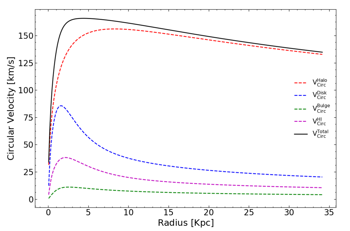
Figure 3: Radial circular velocity profile of the same galaxy showed in Figure 2 (solid line), highlighting the contribution of all the components: stellar and gaseous disc, bulge and halo of the galaxy of, as labelled (see $\S$ 3.2 for details). The velocity profile of this galaxy is dominated by DM at all radii.

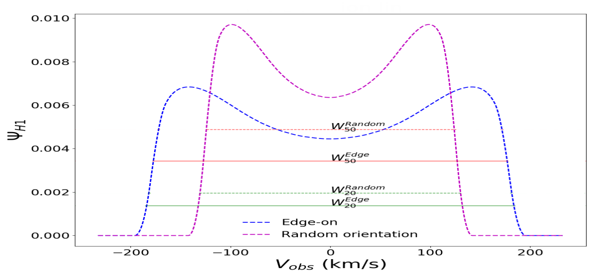
Figure 4: Normalised Hi emission line profile for the same example galaxy of Figs. 2 and 3, with edge-on and intrinsic inclination of the randomly selected galaxy (in this case, $\rm cos\Theta\sim 60^{\circ}$), as labelled. The two top and the two bottom horizontal lines mark the $W_{50}$ and $W_{20}$ of the two orientations respectively. $W_{50}$ and $W_{20}$ are maximal at edge-on orientations.

3.3 Emission Line Profile

To construct the Hi emission line associated with any circular velocity profile, we consider the line profile of a flat ring with constant circular velocity $V_{\rm c}$ and a normalized flux.

After imposing the normalization condition $\int dV_{\rm obs}\tilde{\psi}(V_{\rm obs})\equiv 1$, the edge-on line profile of a ring is,

$$\tilde{\psi}(V_{\rm obs},V_{\rm c})=\begin{cases}\frac{1}{\pi\sqrt{V_{\rm c}^{2}-V_{\rm obs}^{2}}}\hskip 30.00005pt\text{if}|V_{\rm obs}|<V_{\rm c}\\ 0,\hskip 65.00009pt\text{otherwise.}\end{cases}$$ (11)

This profile diverges as $|V_{\rm obs}|\rightarrow V_{\rm c}$, but the resulting singularity is smoothed by introducing a constant velocity dispersion for gas of $\sigma_{\rm gas}=10{\rm km}\,{\rm s^{-1}}$ throughout the disc, which mimics the effect of random Hi motions. This assumption is supported by observations of the gas velocity dispersion seen in the nearby galaxies (Leroy et al., 2008). The smoothed normalized velocity profile is then given by

$$\psi(V_{\rm obs},V_{\rm c})=\frac{\sigma^{-1}}{\sqrt{2\pi}}\int dV\ \text{exp}\left[\frac{(V_{\rm obs}-V_{\rm c})^{2}}{-2\sigma^{2}}\right]\ \tilde{\psi}(V_{\rm obs},V_{\rm c}).$$ (12)

From the edge-on line profile $\psi(V_{\rm obs},V_{\rm c})$ of a single ring and the surface density of atomic hydrogen, $\Sigma_{\rm HI}$, which has been calculated as described in $\S$ 3.1, we can construct the edge-on profile of the Hi emission line for the entire Hi disc, by using the following equation,

$$\Psi_{\rm HI}(V_{\rm obs})=\frac{2\pi}{M_{\rm HI}}\int_{0}^{\infty}dr\ r\Sigma_{\rm HI}(r)\psi(V_{\rm obs},V_{\rm c}(r)).$$ (13)

An example of the resulting Hi emission lines is shown in Figure 4, where we can see the signature double-horned profile. We include the effect of inclinations by using the inclination provided by stingray for every galaxy in the lightcone.

To construct the Hi emission lines we assume a constant Hi velocity dispersion. Observations have found the latter to be remarkably constant, with values typically ranging from $8-12$ km s^-1 (Leroy et al., 2008), and approximately independent of galaxy properties. This has been suggested to be caused by thermal motions setting the Hi velocity dispersion, and the Hi abundance being largely dominated by the warm, neutral interstellar medium. Hence, we decide to keep this value constant, but note that increasing (decreasing) $\sigma_{\rm gas}$ has an effect of slightly increasing (decreasing) the number of low $W_{\rm 50}$ galaxies, $\lesssim 40$ km s^-1 in Figure 9.

3.4 Flux calculation

The lines described in $\S$ 3.3 are normalized, and so need to multiply by the integrated flux of the Hi line to approximate an observed Hi emission line, which we do by using the relation of Catinella et al. (2010a),

$$\frac{M_{\rm HI}}{\rm M_{\odot}}=\frac{2.356\times 10^{5}}{1+z}\left[\frac{d_{\rm L}(z)}{\rm Mpc}\right]^{2}\left(\frac{\int\rm Sd\Omega}{\rm Jy\ \rm kms^{-1}}\right);$$ (14)

here $M_{\rm HI}$ is the Hi mass, $d_{L}(z)$ is the luminosity distance of the galaxy at redshift $z$, and $\int\rm Sd\Omega$ is the integrated flux. The luminosity distance and redshift information were obtained from the ALFALFA lightcone produced in the $\S$ 2.1 and the Hi mass is directly output by Shark.

3.5 How well does the Hi velocity width trace $V_{\rm max}$

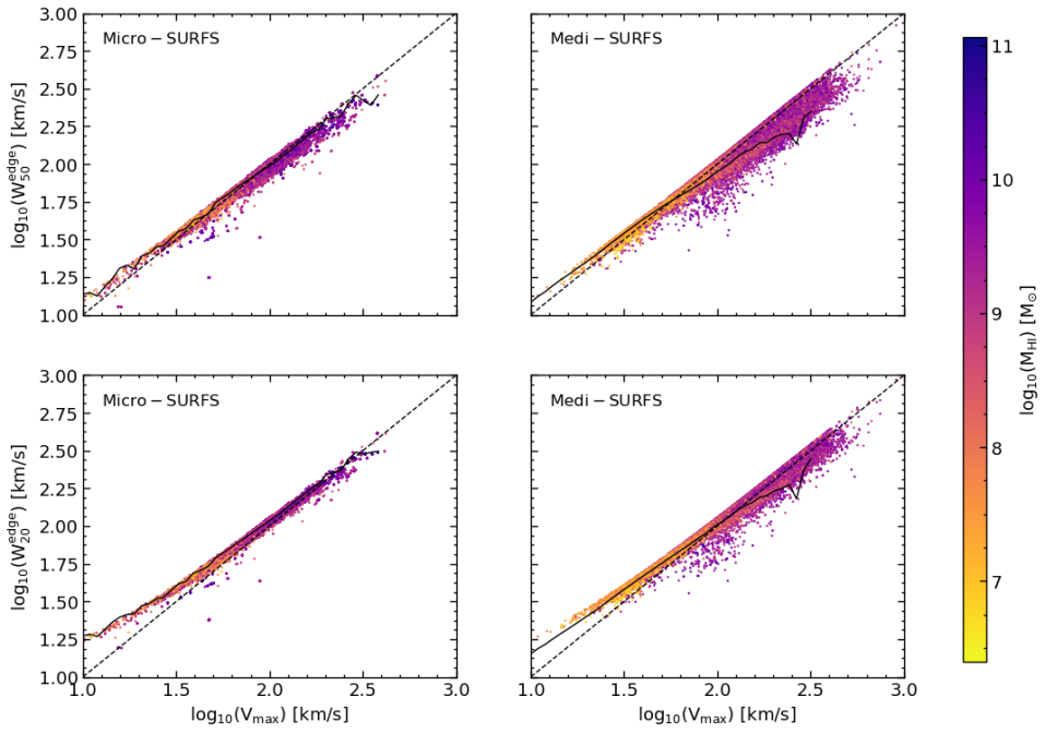
Figure 5: Comparison of the intrinsic maximum circular velocities of Shark galaxies with that derived from our mock observations of the galaxies, using the width at $50$% (top row) and $20$% (bottom row) of the peak flux of the Hi emission lines of the simulated galaxies. The dashed and solid lines represent the 1:1 line and median of the values, respectively, with each scatter point being an individual galaxy in the simulation, and coloured by their Hi mass, as shown in the colour bar at the right of the figure. A slight tendency to deviate up from the 1:1 relation is seen at $V_{\rm mas}\lesssim 30\,$ km s^-1, which is caused by the fact that the Hi velocity dispersion and rotational velocity become comparable at such low velocities. As $W_{20}$ is measured at a lower level than $W_{50}$ it gets affected more by the dispersion than $W_{50}$.

Figure 5 compares $V_{\rm{max}}$ and the $50^{\rm th}$ percentile, $W_{50}$, and $20^{\rm th}$ percentile, $W_{20}$, widths of the Hi emission lines in the case of edge-on orientations, for all galaxies in the ALFALFA lightcone (see $\S$3.2 for a description of $V_{\rm{max}}$); $W_{50}$ and $W_{20}$ are widely used in the observations to estimate rotational velocities of galaxies.

Figure 5 shows that there is good agreement between the true maximum circular velocities and the simulated Hi $W_{50}$ and $W_{20}$ at the higher velocity regime, $V_{\rm max}\gtrsim 100\,$ km s^-1, but there are systematic deviations at lower velocities, $V_{\rm max}\lesssim 35\,$ km s^-1. These deviations can be understood as the effect of non-circular motions modelled via the inclusion of the random Hi velocity component to the Hi emission lines. As stated in $\S$ 3.3, we incorporate a velocity dispersion of $10$  km s^-1 throughout the Hi disc. When we reach the low velocity range ($\lesssim 35$  km s^-1), this velocity dispersion is comparable to these circular velocity of the disc and skews the Hi linewidths. We should also note that the direction of this skewness is the opposite to what Brooks et al. (2017) found in their cosmological hydrodynamical zoom simulations of dwarf to MW galaxies. In spite of this effect, however, we can recover the observed Hi velocity and mass distributions $\S$ 4.2.

3.6 Hi line profiles: Idealised models vs. Hydrodynamical simulations

As discussed in $\S$ 3, we assume profiles for our dark matter, gas and stellar components when modelling the Hi emission lines of all Shark galaxies. In addition, we also assume axis-symmetry that leads to perfect double-horned Hi emission line profiles for our Shark galaxies. Observations show that asymmetries in the Hi  emission line profiles are common (Catinella et al., 2010b) and hence we would like to test how much our assumptions affect our ability to predict a distribution of $W_{50}$ and $W_{20}$.

With this aim, we use a suite of 13 dwarf and 2 Milky-Way sized galaxies from the APOSTLE cosmological hydrodynamical simulations suite (Sawala et al., 2016) as a test-bed, and use the MARTINI (Oman et al., 2019) software to produce Hi  emission lines for all these galaxies (see Appendix A for details). We find that our idealised model reproduces very well the $W_{20}$  measurements of the APOSTLE simulations. However, the $W_{50}$ measurements show more discrepancies driven by the asymmetry of the Hi emission lines in the APOSTLE simulations. These deviations are typically within $\approx 25$% in the case of dwarf galaxies $V_{\rm max}\lesssim 100$  km s^-1, while being larger for the $2$ Milky-Way galaxies. Because we are interested primarily in the dwarf regime, we conclude that our idealised HI emission line model produces a good enough representation of dwarf galaxies even in hydrodynamical simulations.

4 Reproducing the Hi masses and velocities of observed galaxies in a $\Lambda$CDM  framework

We compare Shark predictions with Hi observations to highlight the conclusions one could draw in such case. We then go onto comparing our simulated ALFALFA survey with the real one and discuss our findings.

4.1 A raw comparison between Shark and the observed Hi masses and velocities of galaxies

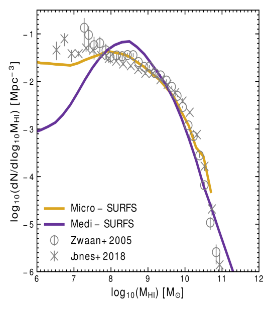
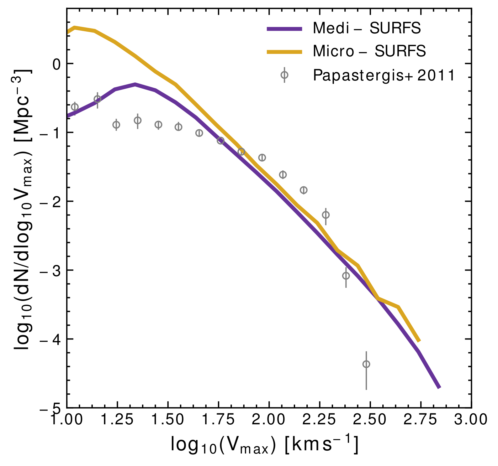
Figure 6: The Hi mass function (left panel) and Hi velocity function (right panel) of all the Shark galaxies at $z=0$, produced using the medi-surfs and micro-surfs, as labelled in each panel. We also show as symbols the observational estimates from Zwaan et al. (2005); Jones et al. (2018) in the case of the Hi mass function, and from Papastergis et al. (2011) for the Hi velocity function. There is good agreement between the Shark and the observations of the Hi mass function, while there is a clear tension with the observations of the Hi velocity function at $V_{\rm mas}\lesssim 100\,$ km s^-1

.

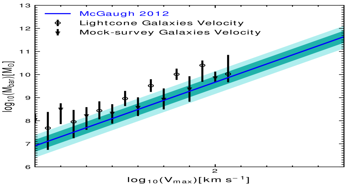
Figure 7: The baryonic Tully-Fisher relation of all the galaxies in the lightcone compared to those that we flag as “ALFALFA-selected” in the lightcone. We also show the best fit to the observed relation from McGaugh (2011). We show the results from the micro-surfs box only as there was little difference in the values from medi-surfs. The figure shows that the entire galaxy population follows a Tully-Fisher relation in tension with the observations, while the more fair comparison with the “ALFALFA-selected” simulated galaxies shows much better agreement, showing that Shark galaxies reproduce the Tully-Fisher relation very well.

The traditional way in which simulations are compared to observations is by taking the predicted galaxy population in the simulated box and comparing directly with derived properties of galaxies in observational surveys. The drawback of such an approach is that there may be important selection biases that are not taken into consideration. This could lead us to conclude that the simulation fails to reproduce an observable when in fact it reflects a mismatch in the different selections and biases that are present in simulation and observational data. This hampers interpretation of the shortcomings of simulations and our understanding of galaxy formation.

In this context, we examine the raw Shark predictions with the derived ALFALFA Hi mass and velocity functions, which should illustrate the importance of accounting for selection effects. We do the comparison using both the micro-surfs and medi-surfs (see $\S$ 2 for details) simulations, and perform a raw comparison with ALFALFA. This assumes that observations are able to sample an unbiased portion of the galaxy population across the probed dynamic range and hence, a reliable volume correction can be applied to take the observed distributions to convert them into functions.

In the left panel of Figure 6, we compare the Hi mass function at $z=0$ that we derive from Shark, running over the two simulation boxes described in $\S$ 1, with the observed Hi  mass function at $z=0$ from Jones et al. (2018) and Zwaan et al. (2005), and find overall agreement between the predictions and observations. Micro-surfs agrees better with the observations across the whole dynamic range of masses observed, while medi-surfs agrees well with the observations at $M_{\rm HI}\gtrsim 10^{9}\,\rm M_{\odot}$, while deviating at lower Hi masses. This difference is simply a resolution effect, in which the haloes that host central galaxies with $M_{\rm HI}\lesssim 10^{9}\,\rm M_{\odot}$ are not well resolved in medi-surfs, but they are in micro-surfs. The median halo mass for central galaxies of $M_{\rm HI}\lesssim 10^{9}\,\rm M_{\odot}$ is $M_{\rm Halo}\lesssim 10^{11.4}\,\rm M_{\odot}$ in the medi-surfs, which would comprise of $\sim 1100$ particles in them. On the other hand, micro-surfs has a similar median halo mass for central galaxies below $M_{\rm\textsc{Hi}}\lesssim 10^{9}\,\rm M_{\odot}$, but because of better mass resolution such halo masses ae made of $\approx 6000$ particles, and so is able to better resolve the haloes over the dwarf galaxy mass range. The agreement between Shark and observations is not surprising because Lagos et al. (2018) used the Hi mass function as a guide to find a suitable set of values for the free parameters in Shark.

In the right panel of Figure 6, we show the comparison between the $40$% ALFALFA data release global Hi velocity function at $z=0$ as calculated by Papastergis et al. (2011) and the “raw” Hi  velocity functions of the circular velocities of the galaxies at $z=0$ in Shark, again for our two simulations, medi-surfs and micro-surfs. This allows us to determine whether or not Shark over-predicts the number of low dynamical mass systems as reported in Zavala et al. (2009), Schneider et al. (2017), Papastergis et al. (2011) and Obreschkow et al. (2013). We find that more galaxies are predicted than are observed by more than an order of magnitude at circular velocities $<100\,\rm km\,s^{-1}$. The peak of the velocity function for micro-surfs is shifted towards a lower velocity ($\sim 20$ km s^-1) due to its higher mass resolution, which enables us to better sample the low dynamical mass galaxies at the cost of producing a smaller number of massive galaxies. The latter is due to the smaller volume. This problem is remedied by including medi-surfs, which allows us to access much larger cosmological volumes and hence higher dynamical masses. The downside is that its resolution is coarser and hence does not go down to the low halo masses that we have access to with micro-surfs. The two simulations in combination allow us to fully sample the velocity and Hi mass range of interest, $\approx 20$  km s^-1 to $800$  km s^-1. We confirm previous results that have reported an over-abundance of low-dynamical mass galaxies in $\Lambda$CDM compared to observations, even after accounting for the complexity of how galaxies populate haloes through the modelling of Shark.

Because we are investigating the masses and velocities of galaxies, it is natural to extend the comparison to the Tully-Fisher relation (Tully & Fisher, 1977), which is an empirical relation between the optical luminosity and the $W_{50}$ of Hi emission lines. The Tully-Fisher relation has been used to place tight constraints on galaxy formation models and is used as a test for the robustness of those models (e.g. Fontanot et al., 2017). McGaugh (2011) extended the classic Tully-Fisher relation to the baryonic Tully-Fisher relation (BTFR), which relates the total baryonic mass of galaxies (gas plus stars) with the observed rotational velocities. In Figure 7, we compare the predicted BTFR of all disc-dominated (bulge-to-total ratio $<0.5$) Shark galaxies (open symbols) with the observed BTFR of (McGaugh, 2011). Here, we only show the micro-surfs because the medi-surfs results are similar, albeit lacking the lowest $V_{\rm circ}$ galaxies. We find that the simulated galaxies tend to be $\approx 0.2-0.3$ dex more Hi massive at fixed circular velocity compared to observations. If instead we use the edge-on Hi $W_{50}$ of galaxies that are present in our mock survey, we find that they follow the BTFR more closely. This result further strengthens our confidence in that the Hi $W_{50}$ measurements done in this study are a closer representation of the observed Hi $W_{50}$ than raw circular velocity.

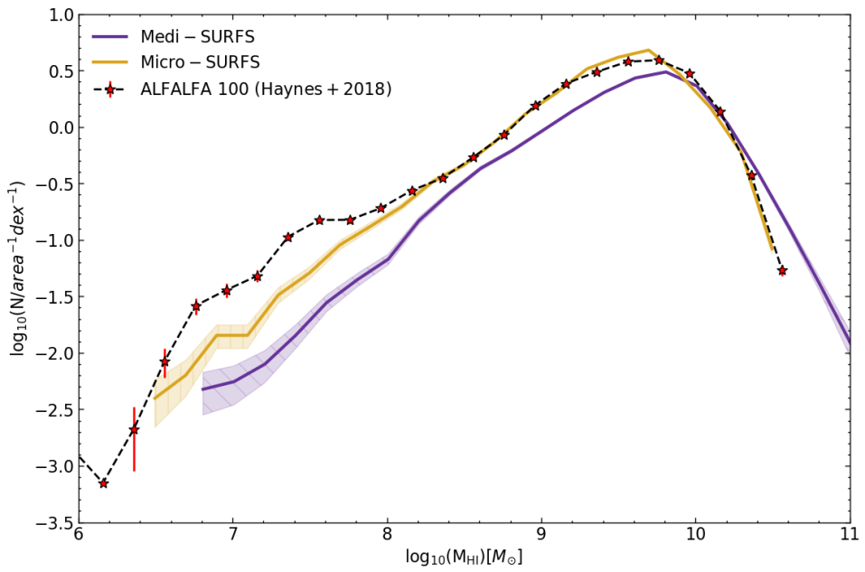
Figure 8: Comparison of the Hi mass distribution as obtained from our mock ALFALFA survey with the observations of Haynes et al. (2018). The purple and yellow solid lines represent the results of the lightcones constructed with Shark, using the medi-surfs and micro-surfs $N$-body simulations, respectively. The shaded region is representative of the poisson noise in the data. Our mock survey’s Hi mass distribution, in both resolution boxes, is in reasonable agreement with the observations.

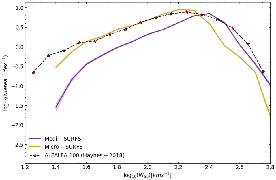
Figure 9: The Hi velocity distribution obtained by our mock ALFALFA survey, with the purple and yellow solid lines representing the Shark model run over the medi- and micro-surfs simulations, respectively, with the shaded regions representing the poisson noise. Because micro-surfs has a higher resolution than medi-surfs, it traces the lower velocity end better, while the medi-surfs is able to track down the galaxies at higher velocity end. By combining the results from these two boxes and applying the selection function of ALFALFA, we are able to obtain a velocity function that is in agreement with the observations.

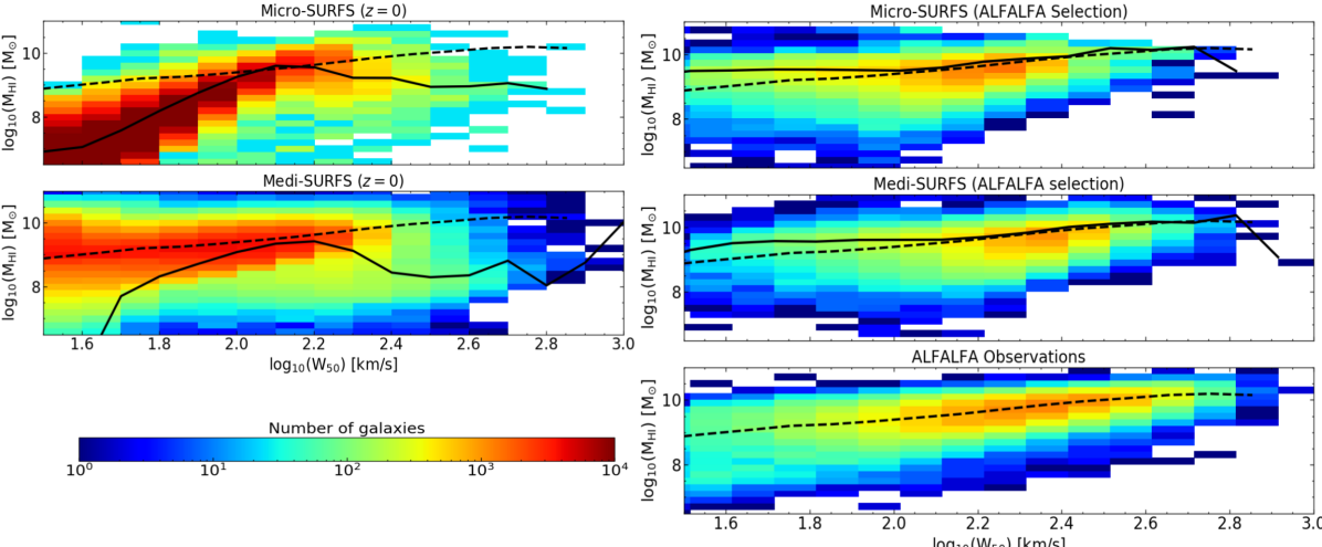
Figure 10: 2D histograms showing the number of galaxies in the plane of Hi mass and $W_{50}$ for the Shark galaxies obtained by running the model in the medi-surfs and micro-surfs, as labelled. The left-hand panels show all the galaxies in the simulation at $z=0$, which we scale accordingly to match the volume of ALFALFA, whereas the right-hand panels show only the galaxies that are comply with the ALFALFA selection in our mock survey. The bottom, right-hand panel shows the actual observed Hi mass-$W_{50}$ relation of the ALFALFA survey as released in Haynes et al. (2018). The colour bar indicates the number of galaxies present in each bin. Solid lines show the running median for that respective panel whereas the dashed line is the running median for the ALFALFA observations. Most galaxies in the model are below the ALFALFA selection criterion which is why the relations look so different between the left and right panels. Anyhow, the similarity to the actual observations gives us the confidence that we are detecting similar galaxies in our mock survey.

Figure 11: Half-gas mass disc radius (left panel) and Hi-to-stellar mass ratio (right) as a function of stellar mass of the galaxies at $z=0$ in Shark. The lines and colours represent our two simulations medi- and micro-surfs, as labelled. Shaded regions show the $16^{\rm th}-84^{\rm th}$ percentiles. For clarity, the latter are shown only for the medi-surfs. A clear selection effect is seen as galaxies with larger gas discs and higher gas-to-star ratio are preferentially selected by ALFALFA.

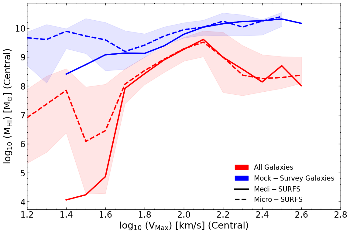
Figure 12: Left: Hi content of galaxies as a function of the maximum circular velocity of the galaxy (which is used as a proxy for dynamical mass). Due to the limited resolution of medi-surfs, we only shown the latter down to ${\rm log}_{10}(V_{\rm max}/{\rm km\,s^{-1}})=1.4$. Resolution is the likely driver of the difference seen between medi- and micro-surfs below ${\rm log}_{10}(V_{\rm max}/{\rm km\,s^{-1}})\approx 1.7$. Here, we show the $16^{\rm th}-84^{\rm th}$ percentiles for micro-surfs as it goes down to lower circular velocities. Right: As Figure 11 but for the star-formation rate (SFR) as a function of the stellar mass. In both panels a clear bias is seen as the ALFALFA mock-survey is preferentially selecting galaxies with higher Hi content, albeit a smaller bias is seen for the star formation rate.

4.2 A mock-to-real comparison between Shark and ALFALFA

The Arecibo Legacy Fast ALFA (ALFALFA) survey is a ‘blind’ Hi survey that has mapped nearly $7000$ deg² area in the velocity range $-2000<cz<18,000$  km s^-1, where $c$ is the speed of light and $z$ is the redshift. The survey has identified $\sim 31,500$ extragalactic Hi line sources (Haynes et al., 2018). The detection limit of the survey as described by Papastergis et al. (2011) is a function of the integrated Hi line flux,$S_{\rm int,lim}$, and velocity width $S_{\rm int,lim}/{\rm Jy}~{}{\rm kms}^{-1}=0.06~{}(W_{50}^{0.51}/{\rm kms}^{-1})$.

For our analysis, we apply the same selection of Papastergis et al. (2011) to our lightcones (see $\S$ 2.1 for details) to select ALFALFA-like galaxies; this results in our mock “ALFALFA” survey. We remind the reader that our lightcone has the same survey area and redshift coverage as ALFALFA. We also apply beam confusion to the lightcone prior to applying the selection criterion above.

We construct the Hi mass distribution from the released catalogue of Haynes et al. (2018), and present this as number per unit deg². The resulting observed distribution is shown in Figure 8 as symbols. We perform the same measurement in our mock ALFALFA survey (one for each surfs simulation being used here), which we also show in Figure 8. We find that there is very good agreement between the simulated and observed Hi mass distributions, which is particularly striking for the lightcone based on micro-surfs. This is not surprising, because Figure 8 shows that the predicted Hi mass function agrees well with the measurements of Jones et al. (2018). There is a slight tension between Hi masses of $10^{7}$$\rm{M}_{\odot}$ and $10^{8}$$\rm{M}_{\odot}$, where Shark predicts a slightly lower number of galaxies. Lagos et al. (2018) showed that the abundance of galaxies below the break of the Hi mass function was very sensitive to the adopted parameters in the photo-ionisation model. Lower velocity thresholds, below which haloes are not allowed to cool gas to mimic the impact of a UV background, has the effect of producing a higher abundance of low Hi mass galaxies (see their Appendix A).

In this work we do not attempt to calibrate Shark to reproduce the low-mass end of the Hi mass function but simply to show how our default model performs compared to Hi observations, and to put constraints on the magnitude of the discrepancy (if any) between the predictions and the observations of Hi masses and velocity widths.

We now turn our attention to the Hi $W_{50}$ distribution. We take the Hi $W_{50}$ measurements from Haynes et al. (2018) (which are as observed, and hence there is no attempt to correct by inclination effects), and construct the Hi $W_{50}$ distribution (shown as symbols in Figure 9). We also take our modelled Hi $W_{50}$ (assuming the stingray inclinations for our simulated galaxies) and construct the Hi $W_{50}$ distribution for those that pass the ALFALFA selection criterion for our two lightcones created running Shark on the medi- and micro-surfs (lines in Figure 9, as labelled). We find that the model and the observations agree remarkably well. We remind the reader that the observationally derived Hi velocity function and the $V_{\rm max}$ function of Shark displayed differences of factor $\gtrsim 20$ at velocities $\lesssim 30$  km s^-1 (see Figure 6), while in Figure 9, differences are $\lesssim 50$%. In other words, the “missing dwarf galaxy problem” is not evident. Using the medi- and micro-surfs allow us to probe the entire range of the observations with the micro-surfs simulation probing the lower velocity end $\lesssim 30$ km s^-1, while the medi-surfs allows us to improve significantly the statistics at the high Hi $W_{50}$ end $\gtrsim 100$ km s^-1. With Shark applied to these two simulations, we are able to reproduce the observed Hi $W_{50}$ distribution. The large differences seen between Figure 6 and Figure 9 suggests that there are important selection biases which cannot be easily corrected in the process of taking the observed Hi $W_{50}$ distribution and inferring from there an Hi $W_{50}$ function, which prevent us from making a one-to-one comparison between the predicted $V_{\rm max}$ function from DMO simulations and observations. This highlights the fact that building lightcones to reproduce observational surveys is essential to tackle this problem, and, in their absence, erroneous conclusions could be drawn.

We have so far shown that Shark produces galaxies with the correct Hi mass and $W_{50}$ distributions, but that does not necessarily mean that galaxies of a given Hi mass have the right Hi $W_{50}$. To test this, Figure 10 shows 2D histograms of galaxies in the Hi mass-$W_{50}$ plane. The left panel shows all the galaxies in the simulation at $z=0$, whose numbers are scaled accordingly to match the ALFALFA volume, whereas the right panel shows the galaxies which pass the ALFALFA selection criterion applied to our lightcones. We also show the same 2D histograms of galaxies for the real ALFALFA survey in the bottom, right panel of Figure 10. Going from left to right panels of Figure 10 show that the majority of galaxies that were originally present in simulation box do not satisfy the ALFALFA selection. Large differences are seen between the 2D distributions of the galaxies in the $z=0$ simulated boxes and the mock ALFALFA lightcones. Most of the galaxies in both micro- and medi-surfs with masses $M_{\rm HI}\lesssim 10^{9}\,\rm M_{\odot}$ are selected out, producing a narrower relation between Hi mass and $W_{50}$ than the one followed by the underlying population of simulated galaxies. Our simulated ALFALFA lightcone reproduces well the observed Hi mass and $W_{50}$ relation of ALFALFA. However, there is some tension in the medians as Shark tends to produce $0.1-0.4$ dex too much HI mass at ${\rm log}_{10}(W_{\rm 50}/{\rm km\,s^{-1}})\lesssim 2.1$. This difference is also seen in Figure 8, as the number of galaxies in the simulations is less than the observed one in the regime of ${\rm M_{\rm HI}}\lesssim 10^{8}{\rm M_{\odot}}$.

In Figures 11 and 12, we show the biases the selection criterion of ALFALFA introduces in the galaxy population; in other words, how do ALFALFA-like galaxy properties compare to the underlying galaxy population? In both figures, the red and the blue colours represent all galaxies in the lightcone (prior to any selection) and the ALFALFA mock-survey galaxies (after applying the ALFALFA selection), respectively.

Figure 11 and the right panel of Figure 12 show the half-gas mass disc radius, Hi-to-stellar mass ratio and star-formation rate (SFR) as a function of the galaxy stellar mass, for all galaxies in Shark and selected by the ALFALFA criteria (i.e. those that make up the distributions of Figures 8 and 9). The left panel of Figure 12 compares the Hi content of the galaxies with its dark matter halo circular velocity, for the sub-sample of central galaxies in both Shark and in those selected as ALFALFA-like. When comparing the gas radii (see left panel in Figure 11), we see that the median of the ALFALFA mock survey galaxies is always higher than the overall median of galaxies in Shark (i.e. the underlying galaxy population), with our simulated ALFALFA galaxies having a half-gas mass radius of the disc $\approx 0.5-0.7$ dex larger than Shark galaxies of the same stellar mass at $M_{\star}\lesssim 10^{10.3}$$\rm{M}_{\odot}$. A drop in the half-gas mass radii of galaxies at stellar masses higher than $10^{10.3}$ $\rm{M}_{\odot}$is seen for the overall median of the Shark galaxies (red). The latter is due to this mass range being dominated by passive elliptical galaxies which tend to be gas poor. This drop is not seen in the median of the ALFALFA mock survey galaxies (blue), thus showing that ALFALFA preferentially picks out gas-rich galaxies, avoiding early-type galaxies that are affected by AGN feedback. This preference is clear when we compare the $\frac{M_{\rm HI}}{M_{\star}}$ ratio for both observed and all galaxies in the Shark (see right panel in Figure 11), with the mock ALFALFA survey galaxies, which continue to be systematically gas richer than the overall median, even at the dwarf galaxy regime.

We also see a strong preference for gas-rich galaxies when we compare the maximum circular velocity of central galaxies with their Hi content (see left panel in Figure 12), with the mock observed galaxies median (blue) staying in the range of $10^{8}\rm M_{\odot}\lesssim M_{\rm HI}\lesssim 10^{10}M_{\odot}$, even when the overall median (red) is orders of magnitude below ($M_{\rm HI}\sim 10^{6}-10^{8}\,\rm M_{\odot}$). Even though both ALFALFA and our mock ALFALFA survey detect galaxies with Hi content as low as $10^{6}$$\rm{M}_{\odot}$, the number of those detections are fairly low ($\sim 20-30$ galaxies), making the higher Hi mass galaxies more dominant and skewing the median towards those values even at the low circular velocity end.

When analysing the overall central galaxy population, there is a clear peak in the $M_{\rm HI}-V_{\rm max}$ relation, which is related to the peak of the baryon collapse efficiency in galaxies (e.g. Eckert et al. 2017). Baugh et al. (2019) using the GALFORM semi-analytic model of galaxy formation (Cole et al., 2000; Lacey et al., 2016; Lagos et al., 2014) also found a sharp break in the Hi mass-halo mass relation at $\gtrsim 10^{11.5}\,\rm M_{\odot}$. This is the approximate halo mass scale at which AGN feedback starts to suppress gas cooling in both models, leading to the decline in Hi mass. The width and prominence of the peak is therefore expected to be very sensitive to the AGN feedback model and hence a useful relation to constrain from observations.

When comparing the star formation rate (SFR) with the stellar mass (see right panel in Figure 12), we see only a small tendency for the ALFALFA mock survey galaxies to have slightly higher SFRs than the underlying galaxy population, again across the whole stellar mass range studied here. The most probable reason for this effect is that in Shark the SFR is calculated from the H₂ content of the galaxies, which in turn depends on the total gas mass and radius. Because gas masses are larger in the ALFALFA mock survey galaxies compared to the underlying population, that tends to drive a smaller H₂/HI ratio, which is why the SFRs in Figure 12 are close to the median of Shark despite the higher Hi abundance in Figure 11. The main sequence of star formation of the entire sample of lightcone galaxies shows a clear break at $\sim 10^{10}$$\rm{M}_{\odot}$, driven by the mass above which AGN feedback starts to be important (typically overcoming the gas cooling luminosity). This break is not seen in the ALFALFA mock survey galaxies, showing the strong bias against gas poor, low star-forming galaxies.

These biases are to be expected because ALFALFA is a blind survey and is limited by the integrated Hi flux and velocity width, which in turn depends on the Hi mass content of galaxies. What is unexpected is that these biases are important even at the dwarf galaxy regime, where most galaxies are star-forming and gas-rich; our ALFALFA mock survey galaxies are more gas-rich and more star-forming. This also raises concerns regarding how best to correct for the galaxies that are not detected by ALFALFA, and how to account for the fact that the observed population is not representative even at the dwarf galaxy regime. Thus, we can see that selection bias plays a very important role in our understanding of the intrinsic galaxy properties and are crucial even at dwarf galaxy scales.

4.3 Implications for $\Lambda$CDM and comparisons with previous studies

Brooks et al. (2017) used a suite of $33$ cosmological zoom hydrodynamical simulations, covering a wide dynamic range from dwarfs to MW-like galaxies, and suggested that the dearth of observed galaxies with low circular velocities was caused by the Hi line-width (used as the dynamical mass tracer) not tracing the full potential well in dwarf galaxies. The reason for this was because in their simulated dwarf galaxies, the bulk of HI is in the rising part of the rotation curve, which means that the integrated HI line width does not reflect the maximum circular velocity of the galaxy. This results in a relation between the effective circular velocity of Hi ($V_{\rm HI}=W_{\rm 50}/2$ for a galaxy observed edge-on) and the maximum circular velocity which significantly deviates from the 1:1 relation at the dwarf galaxy regime, in a way that in the latter $V_{\rm HI}$ is much smaller than $V_{\rm max}$. By applying the relation $V_{\rm HI}-V_{\rm max}$ obtained from their zoom simulations to the dark matter halos of a large cosmological volume, DM-only simulation, they were able to reproduce the observed galaxy velocity function. This therefore offers an attractive solution to the tension seen in Figure 6, which is also supported by the fact that there have been reports from observations in some nearby dwarfs that the bulk of HI is indeed in the rising part of the rotation curve e.g. Catinella et al. (2006); Swaters et al. (2009); Oman et al. (2019).

Macciò et al. (2016) arrived at a similar conclusion, but using mock-observed galaxies from the NIHAO simulations suite(a suite of 100 cosmological hydrodynamical simulations zooms, again covering a wide dynamic range from dwarfs to MW-like galaxies Wang et al., 2015). They obtained similar deviations of the $V_{\rm HI}-V_{\rm max}$ relation from the 1:1 line at the dwarf galaxy regime as Brooks et al. Two reasons were given by Macciò et al. (2016) to explain this, one was again the fact that Hi is not extended enough to reach the flat part of the rotation curve, and the second was that the non-circular motions of the gas seem to become significant at the dwarf galaxy regime (also seen in other cosmological zoom simulations; e.g. Oman et al. 2019). Despite this impressive progress, an important limitation remains. Both studies, Macciò et al. (2016) and Brooks et al. (2017), assume their suite of simulated galaxies to be representative of all the galaxies of the same $V_{\rm max}$. The main question is then whether $33$ or $100$ galaxies is sufficient to make a statement about the main drivers of the tension seen in Figure 6.

To address this question we turn to our ALFALFA lightcones and quantify the fraction of galaxies at two maximum circular velocities, $V_{\rm max}=100$  km s^-1 and $V_{\rm max}=30$  km s^-1 that would be selected by ALFALFA (given their selection criteria) in a fixed cosmological volume. These $V_{\rm max}$ values are chosen because the deviations of the $V_{\rm HI}-V_{\rm max}$ relation from the 1:1 line in Macciò et al. (2016); Brooks et al. (2017) appear at $V_{\rm max}\lesssim 100$  km s^-1. In Shark, we find that $\approx 22$% of the galaxies with $V_{\rm max}=100$  km s^-1 would be detectable by ALFALFA, while that number reduces to $\approx 1.4$% for galaxies with $V_{\rm max}=30$  km s^-1. In the context of the simulated samples of Macciò et al. (2016); Brooks et al. (2017), a few galaxies with $V_{\rm max}=100$ km s^-1and $<1$ (or $\sim 0.462$) galaxy with $V_{\rm max}=30$  km s^-1 would be detectable by ALFALFA. In addition, the small fraction of dwarf galaxies that would be detectable by ALFALFA is far from representative of the galaxies that have on average the same stellar or halo mass. This strongly argues for the need of large statistics to assess the tension between $\Lambda$CDM and the observed galaxy velocity function of Figure 6.

Our work therefore differs from previous ones in two fundamental ways. The first is that we use a statistically significant population of galaxies; with each simulated box having $\sim 1.3$ million galaxies, each of which have their own star formation, gas accretion and assembly histories, and so we are capable of simulating the entire ALFALFA survey volume. The second is that is that we obtain a $V_{\rm HI}-V_{\rm max}$ relation that is very close to the 1:1 line even at the dwarf galaxy regime. Hence, we are able to reproduce the observed Hi $W_{50}$ distribution without the need to invoke significant deviations in the $V_{\rm HI}-V_{\rm max}$ relation. That is not to say these deviations do not exist but simply that observations can be reproduced without them. The fact that our model does not obtain the deviations discussed above is likely due to the simplistic physics that is inherent to semi-analytic models, which are much better captured with hydrodynamical simulations, and therefore likely reflects a limitation of our model. In the Appendix, we applied our idealized model to galaxies in the APOSTLE hydrodynamical simulation suite, and found that in dwarf galaxies our method overestimates $W_{50}$ by $\approx 20-30$%. If we were to correct out $W_{50}$ distribution of Figure 9 by these differences, our predicted number of dwarf galaxies would slightly decrease, making the number of dwarfs smaller than the observed one - indicating that the observed abundance of low $W_{50}$ galaxies is very sensitive to baryon physics.

Our work suggests that the main effect in the apparent discrepancies between the predicted $V_{\rm max}$ function from DMO simulations and the recovered one from observations are selection effects, which are complex because of how non-linearly galaxy properties correlate with their halo properties. Hence, the Hi velocity distribution is not a cosmological test, but more appropriately a baryon physics test. This also strongly suggests that for a complete and unbiased understanding of Hi galaxy surveys, it is necessary to mock-observe our simulated galaxy population and compare with observations in a like-to-like fashion.

5 Conclusions

The abundance of galaxies of different maximum circular velocities (the velocity function) is a fundamental prediction of our concurrent cosmological paradigm and hence, of uttermost important to test against observations. In this work, we have used the Shark semi-analytic galaxy formation model to simulate the ALFALFA Hi survey, the largest blind Hi survey to date, to investigate the well-known discrepancy between the observed and predicted galaxy Hi velocity function. Our goal was to determine whether this tension is a true failure of $\Lambda$CDM, or simply a reflection of the complexity of baryon physics.

We have presented how we model Hi emission lines in Shark  taking into account halo, gas and stellar radial profiles of galaxies, and tested our idealised approach against more complex models derived from the cosmological hydrodynamical APOSTLE simulations by comparing our derived Hi line widths with theirs and find good agreement. We used this new modelling to build a mock ALFALFA survey, and in the process, we combined simulation boxes spanning a range of mass resolutions and cosmological volumes, to ensure a good coverage over the full dynamical range probed by the observations. By applying the ALFALFA selection function to our simulated galaxies, we were able to recover the observed Hi velocity and mass distributions to within $30$%, which shows that a physically motivated model of galaxy formation in the $\Lambda$CDM paradigm is able to reproduce the observed Hi velocity width distribution of galaxies. We highlight that these are true predictions of our Shark model, as gas properties are a natural outcome of the model and were not included in fine tuning of the free parameters of the model.

Our key results can be summarised as follows -

• Survey selection plays a major role in explaining the discrepancy between predictions and observations of the HI velocity function. We see an over-prediction of galaxies in the Hi velocity function of more than an order-of-magnitude at the low velocity end only when we make an “out-of-the-box” comparison of the predicted and observed galaxy populations, while a careful comparison accounting for the survey selection criteria reveals discrepancies of less than $50$%. On applying the ALFALFA selection criteria, we get the desired Hi $W_{50}$ distribution even at low circular velocities, alleviating the missing dwarf galaxy problem.

• Our predicted galaxy population agrees well with the observed Hi mass function. We compare the Hi-$W_{50}$ 2D distribution obtained from the $100$% data release of ALFALFA with our mock survey, and find agreement at an acceptable level. This strengthens our belief that the discrepancy between the predicted Hi velocity distribution with the observed one is due to the selection biases inherent in the survey.

• Previous simulations found that the effective HI velocity ($V_{\rm HI}=$$W_{50}$$/2$ for an edge-on galaxy) significantly underestimates $V_{\rm max}$, which has been invoked as a plausible explanation for the discrepancies described above in the velocity function. We find that our HI emission line modelling produces a $V_{\rm HI}-V_{\rm max}$ relation that is very close to the 1:1 line even at the dwarf galaxy regime. Despite this, we are able to reproduce the Hi $W_{50}$ distributions; these deviations may still happen, but we argue that they are not necessary to reproduce the observed Hi $W_{50}$ distribution.

• A clear selection bias is seen when the mock is compared with the total galaxies that are presented in Shark, shown in Figures 11 and 12. The mock ALFALFA survey is biased towards galaxies with a higher Hi gas content, larger Hi sizes and slightly higher SFRs. We find that at fixed $V_{\rm max}$ the mock ALFALFA galaxies are very strongly biased towards high Hi masses, with a difference in the typical Hi mass of up to two orders of magnitude at $V_{\rm max}\approx 30-50$ km s^-1. This selection bias, in turn, affects our understanding of the distribution of galaxies in our local universe. Thus in order to fully understand galaxy evolution, a clear understanding of these biases is required.

• By comparing our simple model of HI emission lines with the more complex HI lines obtained in the cosmological hydrodynamical simulation APOSTLE, we find that $W_{20}$ is less affected by the asymmetry that is seen in the Hi emission lines than $W_{50}$, the more commonly used velocity estimator. Thus, robust observational measurements of $W_{20}$ would be extremely useful to constrain the simulations and uncover any tension with the simulations.

Our study suggests that the primary reason for the discrepancy between the Hi velocity function in observations and $\Lambda$CDM simulations are selection effects in HI surveys, which are highly non-trivial to correct for. The latter is due to the fact that the typical galaxy with low circular velocity detected in ALFALFA is far from representative of galaxies of the same stellar or halo mass, particularly at $V_{\rm max}\lesssim 100$  km s^-1, according to our predictions. The observed Hi velocity distribution is therefore an excellent test for the baryon physics included in our cosmological galaxy formation models and simulations rather than a cosmological one.

A new generation of HI surveys is underway in telescopes such as The Australian Square Kilometer Array Pathfinder (ASKAP; Johnston et al. 2008). Examples of those are the Widefield ASKAP L-band Legacy All-sky Blind surveY (WALLABY: Staveley-Smith, 2008) and the Deep Investigation of Neutral Gas Origins (DINGO: Meyer, 2009). The depth of these surveys will certainly lead to improvements over previous HI surveys; however, a careful consideration of systematic effects such as those described here will be necessary to make measurements that can be robustly compared with simulation predictions. Similarly, the exercise of simulating the selection effects of surveys to the detail presented here, will be equally important to identify the areas in which our understanding of galaxy formation and perhaps cosmology need improvement.

Appendix A Assessment of our HI emission line model against the APOSTLE cosmological hydrodynamical simulations

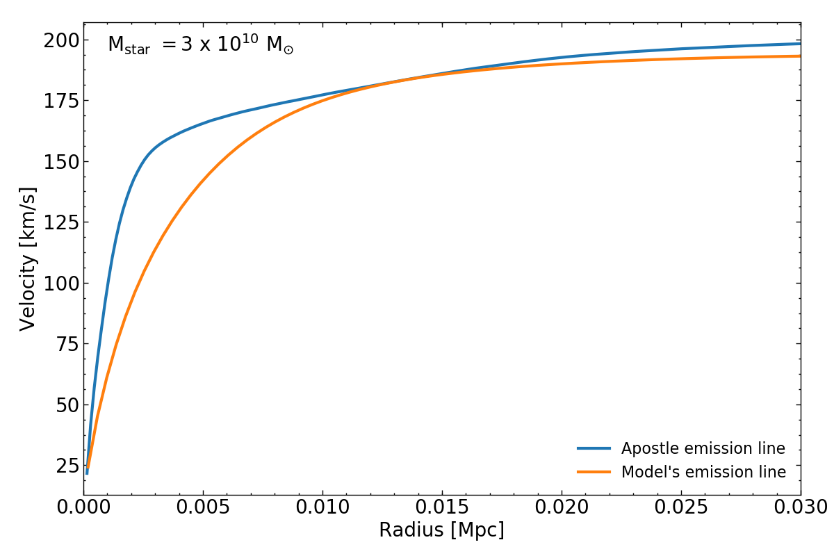
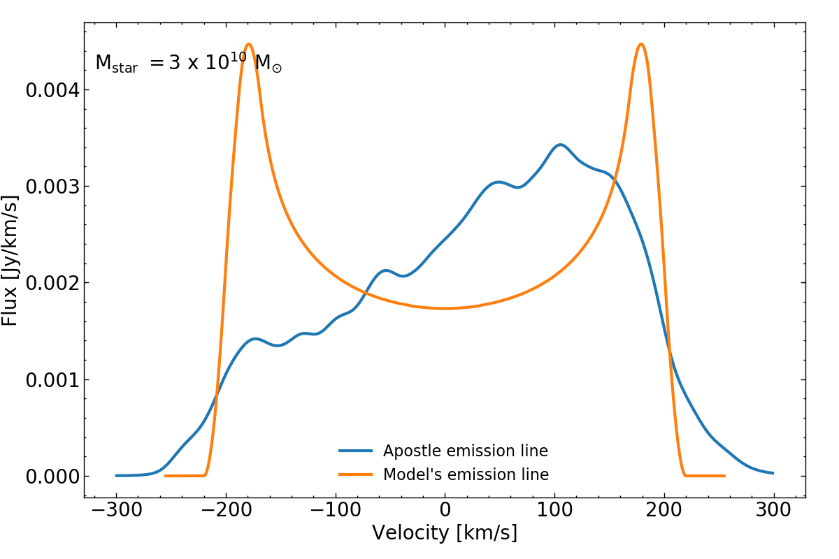
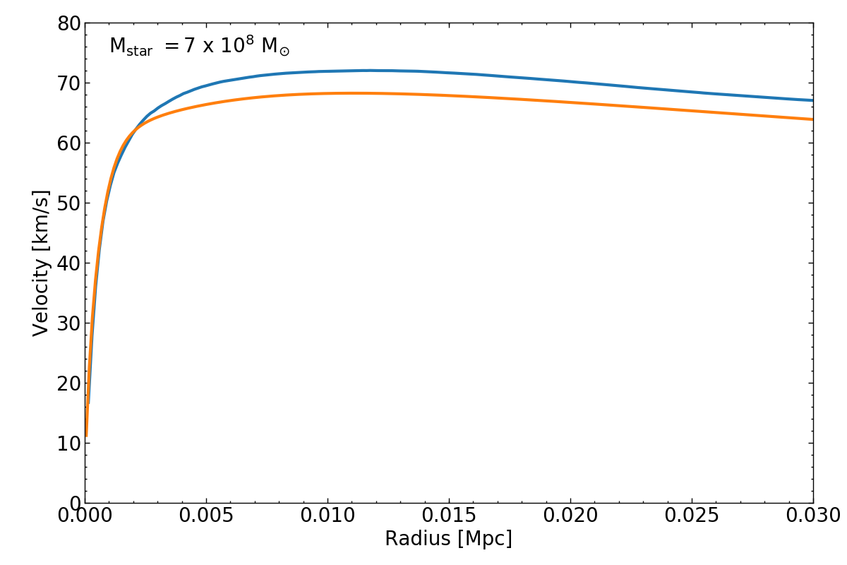
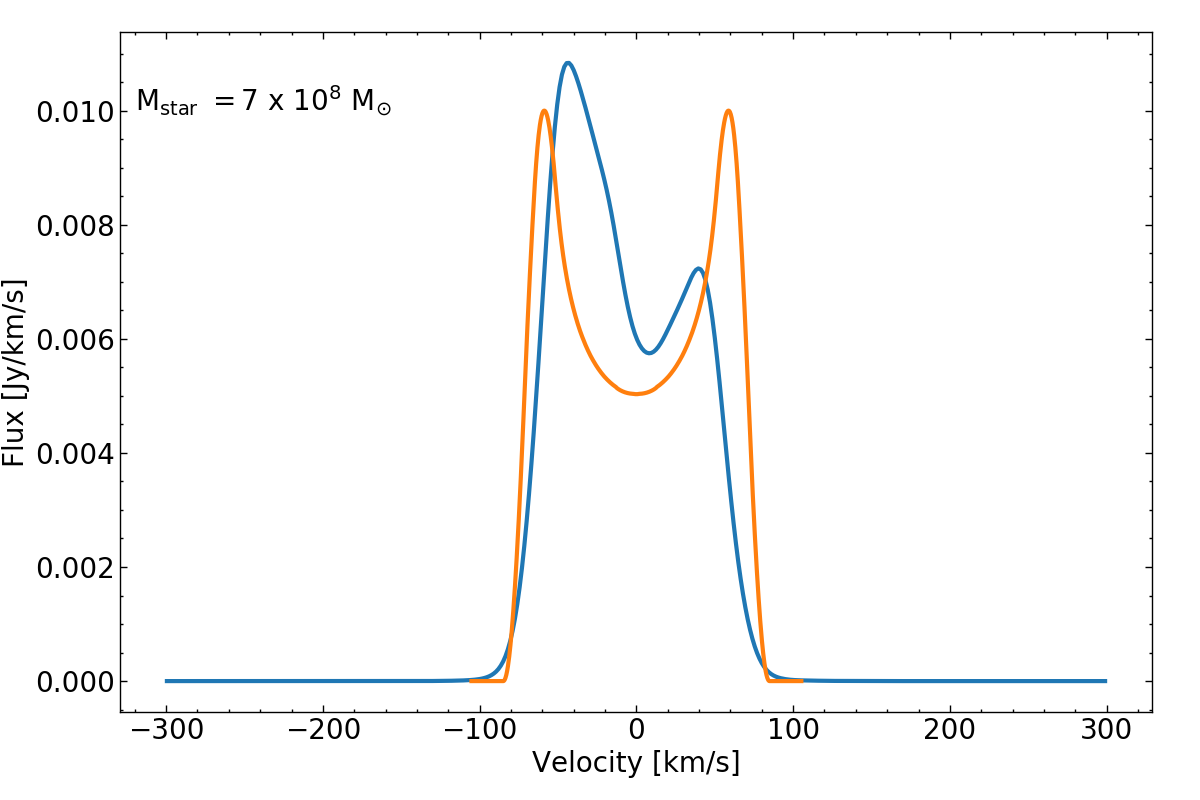
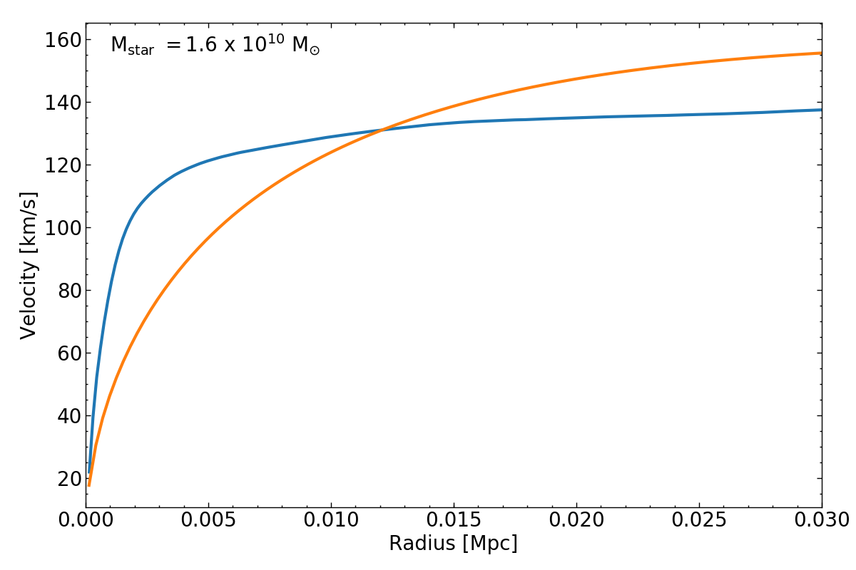
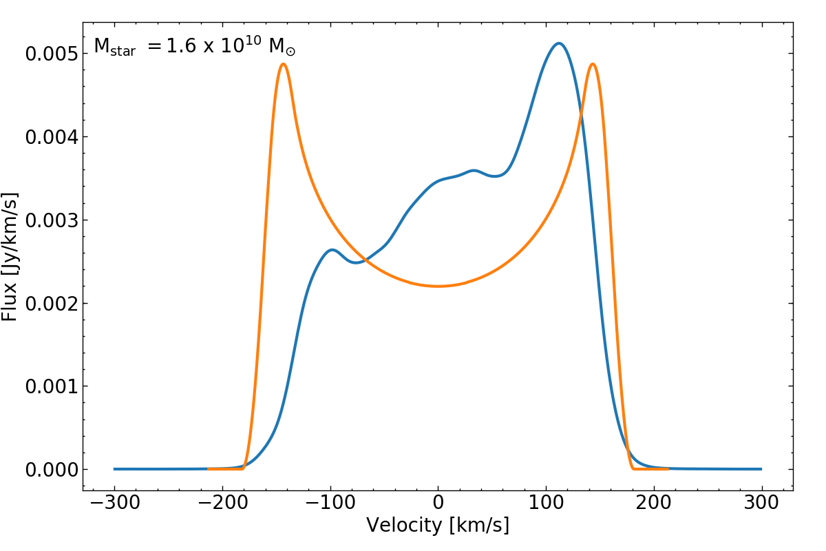
Figure 13: Rotational Velocity curves (left panel) and corresponding Hi emission line profiles (right panel) from the APOSTLE simulations compared to our model. The blue and orange lines correspond to Apostle and our model results, respectively, with the stellar mass of the galaxies as labelled. We show three examples of a galaxy in which our model does poorly (top panel), does well (middle) and an intermediate case (bottom panel).

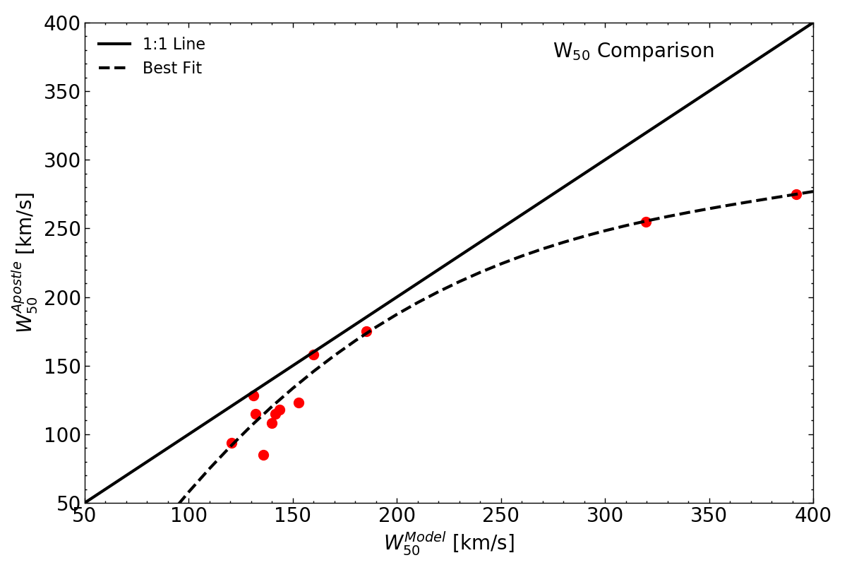
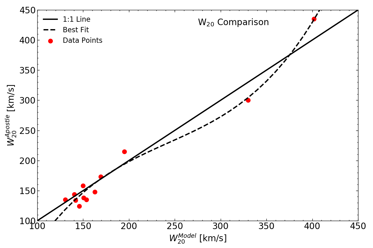
Figure 14: Comparison of the $W_{20}$ and $W_{50}$ measurements taken for the Hi emission lines in APOSTLE and that produced by our idealised model, with the points being individual galaxies, the solid line being the 1:1 ratio and dashed line being the best spline fit. It should be noted that $W_{20}$ measurements agree better between the hydrodynamical simulations and our idealised model than for $W_{50}$. This is because most of the Hi emission line spectra in APOSTLE are asymmetric, which affects $W_{50}$more than $W_{20}$.

The APOSTLE cosmological hydrodynamical simulations (Sawala et al., 2016) are a suite of twelve ‘zoom-in’ volumes evolved with the code and models developed and calibrated for the EAGLE project (Schaye et al., 2015; Crain et al., 2015). The volumes are selected to resemble the Local Group of galaxies in terms of the masses of two central objects – analogous to the Milky Way and M 31, their separation, relative velocity, and relative isolation from other massive systems. Each volume is evolved at 3 resolution levels. The lowest level L3 is similar to the fiducial EAGLE resolution (e.g. L0025N0376 in the nomenclature of Schaye et al., 2015), with a gas particle resolution of $\sim 10^{6}\,{\rm M}_{\odot}$ and gravitational softening of $\sim 700\,{\rm pc}$. The two higher resolution levels each decrease the particle resolution by a factor of $\sim 8$, for a gas particle mass at maximum resolution L1 of $\sim 10^{4}\,{\rm M}_{\odot}$, and a gravitational softening of $\sim 130\,{\rm pc}$. The code uses the ANARCHY implementation Schaller et al. (2015) of pressure-entropy smoothed particle hydrodynamics (Hopkins, 2013), and includes prescriptions for radiative cooling (Wiersma et al., 2009a), an ionizing background (Haardt & Madau, 2001), star formation (Schaye, 2004; Schaye & Dalla Vecchia, 2008), supernovae and stellar mass loss (Wiersma et al., 2009b), energetic feedback from star formation (Dalla Vecchia & Schaye, 2012) and AGN (Booth & Schaye, 2009; Rosas-Guevara et al., 2015). Full details of the model and calibration are available in Schaye et al. (2015); Crain et al. (2015), and of the APOSTLE simulations in Sawala et al. (2016); Fattahi et al. (2016). APOSTLE uses the REFERENCE calibration of the EAGLE model (see Schaye et al., 2015), and the WMAP7 cosmological parameters (Komatsu et al., 2011).

The code martini was used to produce neutral hydrogen (H i) emission line profiles for a selection of galaxies from the APOSTLE simulations. A detailed description of an earlier version is available in Oman et al. (2019). The hydrogen ionization fraction of each simulation particle is estimated following Rahmati et al. (2013); the neutral hydrogen is further partitioned into atomic and molecular gas following Blitz & Rosolowsky (2006). Each particle contributes flux to the spectrum distributed as a Gaussian centered at the particle velocity, with a width specified by $\sqrt{k_{B}T/m_{p}}$, where $k_{B}$ is Boltzmann’s constant, $T$ is the particle temperature, and $m_{p}$ is the particle mass, and an amplitude proportional to the neutral hydrogen mass of the particle. The galaxies are placed edge-on ($i=90^{\circ}$) at a fiducial distance of $D=10\,{\rm Mpc}$, with a systemic velocity of $H_{0}D$, with $H_{0}=70\,{\rm km}\,{\rm s}^{-1}\,{\rm Mpc}^{-1}$. The galaxies are selected morphologically to host gas discs, and to span a range in total (dynamical) mass, with $14$ between $60<V_{\rm max}/{\rm km}\,{\rm s}^{-1}<120$ and $2$ with $V_{\rm max}\sim 200\,{\rm km}\,{\rm s}^{-1}$, where $V_{\rm max}$ is the maximum of the circular velocity curve. Other quantities required as inputs for our model were measured directly from the simulation particle properties – specifically, virial mass of the halo,Hi and stellar mass of galaxy and half-mass stellar and gas radii for the galaxy.

We build Hi emission lines following the procedure described in $\S$ 3 using the input global properties specified above. On the other hand, the Hi emission lines from APOSTLE make full use of the complex geometry and non-circular motions that are predicted by the simulation. We compare our idealised model with the Hi emission lines predicted by APOSTLE with the aim of understanding the systematic effects introduced by our assumptions with respect to more realistic Hi line profiles. We used $13$ dwarf galaxies and $2$ Milky way sized galaxies to compare our models.

In Figure 13, we compare the Hi emission for 3 example galaxies, highlighting cases in which our idealised model provided a poor and a good representation of the Hi emission line (top and middle panels, respectively), with the bottom panel showing an intermediate case.

We find that for some galaxies the estimates of our model and the Hi generated by the simulation show comparable widths and rotation curves but for others our model produces a rotation curve that flattens are smaller radii. When we compare the $W_{50}$ and $W_{20}$ (see Figure 14), we notice that for galaxies with a higher mass or higher velocity and symmetric double-horned profile shape, we produce measurements that are close to the APOSTLE ones. We find better agreement in our $W_{20}$ values than the $W_{50}$ estimates. The cause for this is the asymmetry of the lines in the APOSTLE simulated galaxies, which leads to systematically different $W_{50}$ estimates (due to the heights of the lines), which play a lesser role on $W_{20}$. This suggests that $W_{20}$ should be a more stable, reliable estimate of the dynamical mass, in agreement with the inferences of McGaugh (2011).

The reason why the Hi emission lines in APOSTLE are so asymmetric and whether that agrees with observations is unclear. Oman et al. (2019) studied the velocity profiles of APOSTLE dwarf galaxies, finding significant contribution from non-circular motions in addition to the purely circular velocity. Sales et al. (2017) found that APOSTLE dwarf galaxies may be significantly deviating from the measured Tully-Fisher relation of Papastergis et al. (2016). The latter may be an indication that feedback effects are too strong in APOSTLE. However, further research on the Hi line profiles of APOSTLE galaxies is required before we can make draw robust conclusion.

Equations 15 and 16 show spline fits to the relations shown in Figure 14. These equations could be used as an approximation to the deviations of $W_{50}$ and $W_{20}$ from our idealised model.

$$\begin{multlined}W_{\rm 50_{\rm Apostle}}=6.02\times 10^{-6}\times W_{\rm 50_{\rm Model}}^{3}-7.04\times 10^{-3}\times W_{\rm 50_{\rm Model}}^{2}\\ +2.98\times W_{\rm 50_{\rm Model}}-176.04\end{multlined}W_{\rm 50_{\rm Apostle}}=6.02\times 10^{-6}\times W_{\rm 50_{\rm Model}}^{3}-7.04\times 10^{-3}\times W_{\rm 50_{\rm Model}}^{2}\\ +2.98\times W_{\rm 50_{\rm Model}}-176.04$$ (15)

$$\begin{multlined}W_{\rm 20_{\rm Apostle}}=2.40\times 10^{-5}\times W_{\rm 20_{\rm Model}}^{3}-1.75\times 10^{-2}\times W_{\rm 20_{\rm Model}}^{2}\\ -4.93\times W_{\rm 20_{\rm Model}}-280.69\end{multlined}W_{\rm 20_{\rm Apostle}}=2.40\times 10^{-5}\times W_{\rm 20_{\rm Model}}^{3}-1.75\times 10^{-2}\times W_{\rm 20_{\rm Model}}^{2}\\ -4.93\times W_{\rm 20_{\rm Model}}-280.69$$ (16)

References

- Baugh (2006) Baugh C. M., 2006, Reports on Progress in Physics, 69
- Baugh et al. (2019) Baugh C. M., et al., 2019, MNRAS, 483, 4922
- Blitz & Rosolowsky (2004) Blitz L., Rosolowsky E., 2004, ApJ, 612, L29
- Blitz & Rosolowsky (2006) Blitz L., Rosolowsky E., 2006, ApJ, 650, 933
- Booth & Schaye (2009) Booth C. M., Schaye J., 2009, MNRAS, 398, 53
- Boylan-Kolchin et al. (2011) Boylan-Kolchin M., Bullock J. S., Kaplinghat M., 2011, MNRAS, 415, L40
- Brooks et al. (2017) Brooks A. M., Papastergis E., Christensen C. R., Governato F., Stilp A., Quinn T. R., Wadsley J., 2017, ApJ, 850, 97
- Bull et al. (2016) Bull P., et al., 2016, Physics of the Dark Universe, 12, 56
- Bullock & Boylan-Kolchin (2017) Bullock J. S., Boylan-Kolchin M., 2017, Annual Review of Astronomy and Astrophysics, 55, 343
- Catinella et al. (2006) Catinella B., Giovanelli R., Haynes M. P., 2006, ApJ, 640, 751
- Catinella et al. (2010a) Catinella B., et al., 2010a, MNRAS, 403, 683
- Catinella et al. (2010b) Catinella B., et al., 2010b, MNRAS, 403, 683
- Cole et al. (2000) Cole S., Lacey C., Baugh C., Frenk C., 2000, MNRAS
- Crain et al. (2015) Crain R. A., et al., 2015, MNRAS, 450, 1937
- Dalla Vecchia & Schaye (2012) Dalla Vecchia C., Schaye J., 2012, MNRAS, 426, 140
- Davies et al. (2018) Davies L. J. M., et al., 2018, MNRAS
- Duffy et al. (2008) Duffy A. R., Schaye J., Kay S. T., Dalla Vecchia C., 2008, MNRAS: Letters, 390, L64
- Duffy et al. (2010) Duffy A. R., Schaye J., Kay S. T., Vecchia C. D., Battye R. A., Booth C. M., 2010, MNRAS, 405, no
- Dutton et al. (2016) Dutton A. A., et al., 2016, MNRAS, 461, 2658
- Dutton et al. (2018) Dutton A. A., Macciò A. V., Buck T., Dixon K. L., Blank M., Obreja A., 2018, arXiv e-prints
- Eckert et al. (2017) Eckert K. D., et al., 2017, ApJ, 849, 20
- Elahi et al. (2018) Elahi P. J., Welker C., Power C., Lagos C. d. P., Robotham A. S. G., Cañas R., Poulton R., 2018, MNRAS, 475, 5338
- Elahi et al. (2019b) Elahi P. J., Poulton R. J. J., Tobar R. J., Lagos C. d. P., Power C., Robotham A. S. G., 2019b, arXiv e-prints
- Elahi et al. (2019a) Elahi P. J., Cañas R., Tobar R. J., Willis J. S., Lagos C. d. P., Power C., Robotham A. S. G., 2019a, arXiv e-prints
- Elmegreen (1989) Elmegreen B. G., 1989, ApJ
- Fattahi et al. (2016) Fattahi A., et al., 2016, MNRAS, 457, 844
- Fontanot et al. (2017) Fontanot F., Hirschmann M., De Lucia G., 2017, ApJ, 842, L14
- Giovanelli et al. (2005) Giovanelli R., et al., 2005, AJ, 130, 2613
- Gonzalez et al. (2000) Gonzalez A. H., Williams K. A., Bullock J. S., Kolatt T. S., Primack J. R., 2000, ApJ, 528, 145
- Haardt & Madau (2001) Haardt F., Madau P., 2001, in Neumann D. M., Tran J. T. V., eds, Clusters of Galaxies and the High Redshift Universe Observed in X-rays. p. 64 (arXiv:astro-ph/0106018)
- Hargis et al. (2014) Hargis J. R., Willman B., Peter A. H. G., 2014, ApJ, 795, L13
- Haynes et al. (2018) Haynes M. P., et al., 2018, ApJ, 861, 49
- Hopkins (2013) Hopkins P. F., 2013, MNRAS, 428, 2840
- Johnston et al. (2008) Johnston S., et al., 2008, Experimental Astronomy, 22, 151
- Jones et al. (2018) Jones M. G., Haynes M. P., Giovanelli R., Moorman C., 2018, MNRAS, 477, 2
- Klypin et al. (2014) Klypin A., Karachentsev I., Makarov D., Nasonova O., 2014, MNRAS
- Komatsu et al. (2011) Komatsu E., et al., 2011, ApJS, 192, 18
- Kregel et al. (2002) Kregel M., Van Der Kruit P. C., Grijs R. d., 2002, MNRAS, 334, 646
- Lacey et al. (2016) Lacey C. G., et al., 2016, MNRAS, 462, 3854
- Lagos et al. (2014) Lagos C. d. P., et al., 2014, MNRAS, 443
- Lagos et al. (2018) Lagos C. d. P., Tobar R. J., Robotham A. S. G., Obreschkow D., Mitchell P. D., Power C., Elahi P. J., 2018, MNRAS, 481, 3573
- Leroy et al. (2008) Leroy A. K., Walter F., Brinks E., Bigiel F., de Blok W. J. G., Madore B., Thornley M. D., 2008, AJ
- Macciò et al. (2012) Macciò A. V., Paduroiu S., Anderhalden D., Schneider A., Moore B., 2012, MNRAS, 424, 1105
- Macciò et al. (2016) Macciò A. V., Udrescu S. M., Dutton A. A., Obreja A., Wang L., Stinson G. R., Kang X., 2016, Monthly Notices of the Royal Astronomical Society: Letters
- McGaugh (2011) McGaugh S., 2011, AJ
- Merson et al. (2013) Merson A. I., et al., 2013, MNRAS, 429, 556
- Meyer (2009) Meyer M., 2009, in Panoramic Radio Astronomy: Wide-field 1-2 GHz Research on Galaxy Evolution. p. 15 (arXiv:0912.2167)
- Meyer et al. (2004) Meyer M. J., et al., 2004, MNRAS, 350, 1195
- Navarro et al. (1995) Navarro J. F., Frenk C. S., White S. D. M., 1995, MNRAS, 275, 720
- Obreschkow et al. (2009a) Obreschkow D., Croton D., De Lucia G., Khochfar S., Rawlings S., 2009a, ApJ
- Obreschkow et al. (2009b) Obreschkow D., Heywood I., Klöckner H. R., Rawlings S., 2009b, ApJ, 702, 1321
- Obreschkow et al. (2009c) Obreschkow D., Klöckner H. R., Heywood I., Levrier F., Rawlings S., 2009c, ApJ, 703, 1890
- Obreschkow et al. (2013) Obreschkow D., Ma X., Meyer M., Power C., Zwaan M., Staveley-Smith L., Drinkwater M. J., 2013, ApJ
- Oman et al. (2015) Oman K. A., et al., 2015, MNRAS, 452, 3650
- Oman et al. (2019) Oman K. A., Marasco A., Navarro J. F., Frenk C. S., Schaye J., Benítez-Llambay A., 2019, MNRAS, 482, 821
- Papastergis et al. (2011) Papastergis E., Martin A. M., Giovanelli R., Haynes M. P., 2011, ApJ, 739, 38
- Papastergis et al. (2016) Papastergis E., Adams E. A. K., van der Hulst J. M., 2016, A&A, 593, A39
- Planck Collaboration et al. (2016) Planck Collaboration et al., 2016, A&A, 594, A13
- Plummer (1911) Plummer H. C., 1911, MNRAS, 71, 460
- Poulton et al. (2018) Poulton R. J. J., Robotham A. S. G., Power C., Elahi P. J., 2018, Publ. Astron. Soc. Australia, 35
- Rahmati et al. (2013) Rahmati A., Pawlik A. H., Raičević M., Schaye J., 2013, MNRAS, 430, 2427
- Rosas-Guevara et al. (2015) Rosas-Guevara Y. M., et al., 2015, MNRAS, 454, 1038
- Sales et al. (2017) Sales L. V., et al., 2017, MNRAS, 464, 2419
- Sawala et al. (2016) Sawala T., et al., 2016, MNRAS, 457, 1931
- Schaller et al. (2015) Schaller M., Dalla Vecchia C., Schaye J., Bower R. G., Theuns T., Crain R. A., Furlong M., McCarthy I. G., 2015, MNRAS, 454, 2277
- Schaye (2004) Schaye J., 2004, ApJ, 609, 667
- Schaye & Dalla Vecchia (2008) Schaye J., Dalla Vecchia C., 2008, MNRAS, 383, 1210
- Schaye et al. (2015) Schaye J., et al., 2015, MNRAS, 446, 521
- Schneider et al. (2012) Schneider A., Smith R. E., Macciò A. V., Moore B., 2012, MNRAS, 424, 684
- Schneider et al. (2017) Schneider A., Trujillo-Gomez S., Papastergis E., Reed D. S., Lake G., 2017, MNRAS, 470, 1542
- Serra et al. (2010) Serra P., et al., 2010, in Verdes-Montenegro L., Del Olmo A., Sulentic J., eds, Astronomical Society of the Pacific Conference Series Vol. 421, Galaxies in Isolation: Exploring Nature Versus Nurture. p. 49
- Springel et al. (2005) Springel V., et al., 2005, Nature, 435, 629
- Staveley-Smith (2008) Staveley-Smith L., 2008, Astrophysics and Space Science Proceedings, 5, 77
- Swaters et al. (2009) Swaters R. A., Sancisi R., van Albada T. S., van der Hulst J. M., 2009, A&A, 493, 871
- Tollerud et al. (2008) Tollerud E. J., Bullock J. S., Strigari L. E., Willman B., 2008, ApJ, 688, 277
- Trujillo-Gomez et al. (2018) Trujillo-Gomez S., Schneider A., Papastergis E., Reed D. S., Lake G., 2018, MNRAS, 475, 4825
- Tully & Fisher (1977) Tully R. B., Fisher J. R., 1977, A&A, 54, 661
- Walter et al. (2008) Walter F., Brinks E., de Blok W. J. G., Bigiel F., Kennicutt R. C., Thornley M. D., Leroy A., 2008, AJ, 136, 2563
- Wang et al. (2015) Wang L., Dutton A. A., Stinson G. S., Macciò A. V., Penzo C., Kang X., Keller B. W., Wadsley J., 2015, MNRAS, 454, 83
- Welker et al. (2018) Welker C., Power C., Lagos C. d. P., Elahi P. J., Cañas R., Pichon C., Dubois Y., 2018, MNRAS, 482, 2039
- Wiersma et al. (2009a) Wiersma R. P. C., Schaye J., Smith B. D., 2009a, MNRAS, 393, 99
- Wiersma et al. (2009b) Wiersma R. P. C., Schaye J., Theuns T., Dalla Vecchia C., Tornatore L., 2009b, MNRAS, 399, 574
- Zavala et al. (2009) Zavala J., Jing Y. P., Faltenbacher A., Yepes G., Hoffman Y., Gottlöber S., Catinella B., 2009, ApJ, 700, 1779
- Zwaan et al. (2005) Zwaan M. A., Meyer M. J., Staveley-Smith L., Webster R. L., 2005, MNRAS, 359, 30