Drawing Order Diagrams Through Two-Dimension Extension

Abstract

Order diagrams are an important tool to visualize the complex structure of ordered sets. Favorable drawings of order diagrams, i.e., easily readable for humans, are hard to come by, even for small ordered sets. Many attempts were made to transfer classical graph drawing approaches to order diagrams. Although these methods produce satisfying results for some ordered sets, they unfortunately perform poorly in general. In this work we present the novel algorithm DimDraw to draw order diagrams. This algorithm is based on a relation between the dimension of an ordered set and the bipartiteness of a corresponding graph.

1 Introduction

Order diagrams, also called line diagrams or Hasse diagrams, are a great tool for visualizing the underlying structure of ordered sets. In particular they enable the reader to explore and interpret complex information. In such diagrams every element is visualized by a point on the plane. Each edge of the covering relation is visualized as an ascending line connecting its points. These lines are not allowed to touch other points. These strong requirements are often complemented with further soft conditions to improve the readability of diagrams. For example, minimizing the number of crossing lines or the number of different slopes. Another desirable condition is to draw as many chains as possible on straight lines. Lastly, the distance of points to (non-incident) lines should be maximized.

Experience shows that in order to obtain (human) readable drawings one has to balance those criteria. Based on this notion, there are algorithms that produce drawings of order diagrams optimizing towards some of the criteria mentioned above. Drawings produced by such algorithms are sufficient to some extent. However, they may not compete with those created manually by an experienced human. However, such an expert is often not available, too expensive, or not efficient enough to create a large number of order diagrams. Hence, finding efficient algorithms that draw diagrams at a suitable quality is still an open task. An exemplary requiring such algorithms is Formal Concept Analysis (FCA) [10], a theory that can be used to analyze and cluster data through ordering it.

In this work we present a novel approach which does not employ the optimization techniques as described above. For this we make use of the structure and its properties that are already encapsulated in the ordered set. We base our idea on the observation that ordered sets of order dimension two can be embedded into the plane in a natural way. Building up on this we show a procedure to embed the ordered sets of order dimension three and above by reducing them to the two-dimensional case. To this end we prove an essential fact about inclusion-maximal bipartite induced subgraphs in this realm. Based on this we link the naturally emerging $\mathcal{NP}$-hard computation problem to a formulation as a SAT problem instance. Our main contribution with respect to this is Theorem 5.2.

We investigate our theoretical result on different real-world data sets using the just introduced algorithm DimDraw. Furthermore, we note how to incorporate heuristical approaches replacing the SAT solver for faster computations. Finally, we discuss in part surprising observations and formulate open questions.

2 Related Work

Order diagrams can be considered as acyclic (intransitive) digraphs that are drawn upward in the plane, i.e., every arc is a curve monotonically increasing in $y$-direction. A lot of research has been conducted for such upward drawings. A frequently employed algorithm-framework to draw such graphs is known as Sugiyama Framework [22]. This algorithm first divides the set of vertices of a graph into different layers, then embeds each layer on the same $y$-coordinate and minimizes crossings between consecutive layers. Crossing minimization can be a fundamental aesthetic for upward drawings. However the underlying decision problem is known to be $\mathcal{NP}$-hard even for the case of two-layered graphs [6]. A heuristic for crossing reduction can be found in [5]. The special case for drawing rooted trees can be solved using divide-and-conquer algorithms [19]. Such divide-and-conquer strategies can also be used for non-trees as shown in [18]. Several algorithms were developed to work directly on order diagrams. Relevant for our work is the dominance drawing approach. There, comparable elements of the order relation are placed such that both Cartesian coordinates of one element are greater than the ones of the other [12]. Weak dominance drawings allow a certain number of elements that are placed as if they were comparable [13] even when they aren’t. Our approach is based on this idea. Previous attempts to develop heuristics are described in [14]. If an ordered set is a lattice there are algorithms that make use of the structure provided by this. The authors in [21] make use of geometrical representations for drawings of lattices. In [8] a force directed approach is employed, together with a rank function to guarantee the “upward property” is preserved. A focus on additive diagrams is laid out in [9].

3 Notations and Definitions

We start by recollecting notations and notions from order theory [23]. In this work we call a pair $(X,R)$ an ordered set, if $R\subseteq X\times X$ is an order relation on a set $X$, i.e., $R$ is reflexive, antisymmetric and transitive. In this setting $X$ is called the ground set of $(X,R)$. In some cases, we write $(X,{\leq})$ instead of $(X,R)$ throughout this paper. We then use the notations $(a,b)\in{\leq}$, $a\leq b$ and $b\geq a$ interchangeably. We write $a<b$ iff $a\leq b$ and $a\neq b$. Alike, if $b\geq a$ and $b\neq a$, write $b>a$. We say that a pair $(a,b)\in X\times X$ is comparable, if $a\leq b$ or $b\leq a$, otherwise it is incomparable. An order relation on $X$ is called linear (or total) if all elements of $X$ are pairwise comparable. For $(X,{\leq})$ the order relation $L$ on $X$ is called a linear extension of $\leq$, iff $L$ is a linear order and ${\leq}\subseteq L$. If $\mathcal{R}$ is a family of linear extensions of $\leq$ and ${\leq}=\bigcap_{L\subseteq\mathcal{R}}L$, we call $\mathcal{R}$ realizer of $\leq$. The minimal $d$ such that there is a realizer of cardinality $d$ for $(X,{\leq})$ is called its order dimension. We use the denotation of order dimension for ordered sets and order relations interchangeably. For a set $X$ and $\mathcal{C}\subseteq X\times X$ we denote $\mathcal{C}^{-1}:=\{(a,b)\mid(b,a)\in\mathcal{C}\}$. The transitive closure of $R$ is denoted by $R^{+}$.

For our work we consider simple graphs denoted by $(V,E)$, where $E\subseteq\binom{V}{2}$. For an ordered set $(X,{\leq})$, its comparability graph is defined as the graph $(X,E)$, such that $\{a,b\}\in E$, if and only if $a,b\in X$ are comparable. Similary the cocomparability graph (sometimes called incomparability graph) is the graph on $X$ where $\{a,b\}$ is an edge if and only if $a,b\in X$ are incomparable. Two order relations on the same ground set are called conjugate to each other, if the comparability graph of one is the cocomparability graph of the other. We refrain from a formal definition of a drawing of $(X,{\leq})$. However we need to discuss the elements of such drawings used in our work. Each element of the ground set is drawn as a point on the plane. The cover relation is defined as ${\operatorname{cr}(X,{\leq})\coloneqq\{(a,b)\in{\leq}\mid\nexists c\in X:a<c<b\}}$. Each element of the cover relation is drawn as a monotonically increasing curve connecting the points.

From here on some definitions are less common. For $(X,{\leq})$ we denote the set of incomparable elements by $\operatorname{inc}(X,{\leq})$. Two elements $(a,b),(c,d)\in\operatorname{inc}(X,{\leq})$ are called incompatible, if their addition to $\leq$ creates a cycle in the emerging relation, i.e., if there is some sequence of elements $c_{1},\ldots,c_{n}\in X$, such that each pair ${(c_{i},c_{i+1})\in{\leq}\cup(a,b)\cup(c,d)}$ with $i\in\{1,\ldots,n\}$ and $c_{n+1}=c_{1}$. We call the graph $((\operatorname{inc}(X,{\leq}),E)$ with $\{(a,b),(c,d)\}\in E$, iff $(a,b)$ and $(c,d)$ are incompatible the transitive incompatibility graph. Denote this graph by $\operatorname{tig}(X,{\leq})$. We say a pair $(a,b)\in\operatorname{inc}(X,{\leq})$ enforces another pair $(c,d)\in\operatorname{inc}(X,{\leq})$, iff $(c,d)\in({\leq}\cup(a,b))^{+}$. If and $(a,b)$ enforces $(c,d)$ in $\leq$, we write $(a,b)\rightarrow(c,d)$.

4 Drawing Ordered Sets of Dimension Two

Ordered sets of order dimension 2 have a natural way to be visualized using a realizer by their dominance drawings [12]. Let $(X,{\leq})$ be an ordered set of dimension two. First define the position for each $x\in X$ in a linear extension $L$ as the number of vertices that are smaller, i.e., $\operatorname{pos}_{L}(x)\coloneqq\{y\in X\mid y<x\}$.

Now let $\mathcal{R}=|\{{\leq_{1}},{\leq_{2}}\}|$ be a realizer consisting of two linear extensions of $\leq$. Each element is embedded into a two-dimensional grid at the pair of coordinates $(\operatorname{pos}_{\leq_{1}}(x),\operatorname{pos}_{\leq_{2}}(x))$. Embedding this grid into the plane is done using the generating vector $(-1,1)$ for $x_{1}$ and $(1,1)$ for $x_{2}$. Each point now divides the plane into four quadrants using the two lines that are parallel to $x_{1}$ and $x_{2}$. It holds that $a<b$, if and only if the point $b$ is in the quadrant above the point $a$ by construction. Draw the elements of the cover relation as straight lines. This guarantees that all elements of the cover relation are drawn as monotonically increasing curves. In order to compute such drawings, a preliminary check of the two-dimensionality of the ordered set is required. If so computing a realizer in polynomial time is possible as a result of the following theorem.

Theorem 4.1 (Dushnik and Miller, 1941 [3])

The dimension of an ordered set $(X,{\leq})$ is at most 2, if and only if there is a conjugate order $\leq_{C}$ on $X$. A realizer of $P$ is given by $\leq$ given by $\mathcal{R}=\{{\leq}\cup{\leq_{C}},{\leq}\cup{\geq_{C}}\}$.

In 1977, Golumbic gave an algorithm [11] to check whether a graph is transitive orientable, i.e., whether there is an order on its vertices, such that the graph is exactly the comparability graph of this order. It computes such an order, if it exists. This algorithm runs in $\mathcal{O}(n^{3})$, with $n$ being the number of vertices of the graph. Combining this with Theorem 4.1 provides an algorithm to compute whether an ordered set is two-dimensional. Furthermore, it also returns a realizer, in the case of two-dimensionality. For the sake of completeness, note that there are faster algorithms (as fast as linear) [17]) for computing transitive orientations. However those only work if the graph is actually transitive orientable and return erroneous results otherwise. On a final note, deciding dimension $3$ or larger is known to be $\mathcal{NP}$-complete as shown by Yannakis in 1982 [24]. This is in contrast to the just stated fact about two-dimensional orders.

5 Drawing Ordered Sets of Higher Dimensions

The idea of embedding two-dimensional orders does generalize in a natural way to higher dimensions, i.e., gives us a nice way to embed $n$-dimensional ordered sets into $n$-dimensional space (Euclidean space) by using an $n$-dimensional realizer. However, projecting an ordered set from a higher dimension into the plane turns out to be hard. See, for example, the projections of an ordered set in example Figure 1. For this reason our algorithm makes use of a different method to compute drawings of order diagrams for higher dimensions.

Figure 1: A three-dimensional ordered set embedded – based on its realizer – into three dimensional Euclidean space and then projected into the plane using a parallel projection from multiple angles. Even though the structure of the ordered set is recognizable, the drawings are all not satisfactory.

In short, the main idea of this section is the following: for a given order relation we want to insert some number of additional pairs in order to make it two-dimensional. This allows the resulting order to be drawn using the algorithm for the two-dimensional case described in the previous section. Afterwards we once again remove all the inserted pairs. By construction, the property that if $a<b$, the point $a$ is inserted below $b$ is still preserved. Such drawings are sometimes called weak dominance drawings [13]. However, for each inserted pair $(a,b)$, we obtain two points in the drawing that are drawn as if $a$ and $b$ were comparable. This poses the question for minimizing the number of inserted pairs.

Definition 1

Let $(X,{\leq})$ be an ordered set. A set $\mathcal{C}\subseteq\operatorname{inc}(X)$ is called a two-dimension-extension of $(X,{\leq})$, iff ${\leq}\cup\mathcal{C}$ is an order on $X$ and the ordered set $(X,{\leq}\cup\mathcal{C})$ is two-dimensional.

Such an extension always exists: a linear extension of dimension one always exists. If an order contains exactly one incomparable pair it has dimension two.

It is known to be $\mathcal{NP}$-complete to decide whether an ordered set can be altered to be two-dimensional by inserting $k$ pairs [1]. Hence, we propose an algorithm that tackles the problem for approximating the corresponding optimization problem. The idea of the algorithm is based on the following theorem.

Theorem 5.1 (Doignon et.al., 1984 [2])

The ordered set $(X,{\leq})$ has order-dimension two if and only if $\operatorname{tig}(X,{\leq})$ is bipartite.

Thus, for $(X,{\leq})$ of dimension greater than two, $\operatorname{tig}(X,{\leq})$ is non-bipartite. We want to find a maximal induced bipartite subgraph of $\operatorname{tig}(X,{\leq})$.

Lemma 1

Let $(X,{\leq})$ be an ordered set and $(a,b),(c,d)\in\operatorname{inc}(X,{\leq})$. Then the following are equivalent:

1. $d\leq a$ and $b\leq c$.

2. $(a,b)\rightarrow(d,c)$.

3. $(c,d)\rightarrow(b,a)$.

4. $(a,b)$ and $(c,d)$ are incompatible.

5. $(b,a)$ and $(d,c)$ are incompatible.

Proof

$(i)\Rightarrow(iv)$. Consider the relation $\prec\coloneqq{\leq}\cup(a,b)\cup(c,d)$. This yields $d\prec a\prec b\prec c\prec d$, i.e, $\prec$ contains a cycle. Analogously $(i)\Rightarrow(v)$.
$(iv)\Rightarrow(ii)$. The assumption directly implies that $(d,c)\in({\leq}\cup(a,b))^{+}$ due to the cycle generated by $(a,b)$ and $(c,d)$. By the same argument $(v)\Rightarrow(iii)$.
$(ii)\Rightarrow(i)$. Assume $d\not\leq a$ or $b\not\leq c$. Since $(d,c)\in({\leq}\cup(a,b))^{+}$ it follows $(d,c)\in{\leq}$ which contradicts $(c,d)\in\operatorname{inc}(X,\leq)$. Similarly follows $(iii)\Rightarrow(i)$. $\square$

Recall the definition of $\operatorname{tig}(X,{\leq})$ defined on $\operatorname{inc}(X,{\leq})$ with incompatible pairs being connected. Call a cycle in $\operatorname{tig}(X,{\leq})$ strict, iff for each two adjacent pairs $(a,b)$ and $(c,d)$ it holds that $d<a$ and $b<c$. A strict path is defined analogously.

Lemma 2 (Doignon et al., [2])

Let $(X,{\leq})$ be an ordered set and let the pair $v\in\operatorname{inc}(X,{\leq})$. Then the following statements are equivalent:

1. $v$ is in contained in an odd cycle in $\operatorname{tig}(X,{\leq})$.

2. $v$ is contained in a strict odd cycle in $\operatorname{tig}(X,{\leq})$.

Remark 1

This is stated implicitly in their proof of Proposition 2, verifying the equality between the two chromatic numbers of a hypergraph corresponding to our cycles and a hypergraph corresponding to our strict cycles.

Theorem 5.2

Let $(X,{\leq})$ an ordered set. Let $\mathcal{C}\subseteq\operatorname{inc}(X,{\leq})$ be minimal with respect to set inclusion, such that $\operatorname{tig}(X,{\leq})\backslash\mathcal{C}^{-1}$ is bipartite. Then $(X,{\leq}\cup\mathcal{C})$ is an ordered set.

Proof

Refer to the bipartition elements of $\operatorname{tig}(X,{\leq})\backslash\mathcal{C}^{-1}$ with $P_{1}$ and $P_{2}$.

Claim

The arrow relation is transitive, i.e., if $(a,b)\rightarrow(c,d)$ and $(c,d)\rightarrow(e,f)$ then $(a,b)\rightarrow(e,f)$. If $(a,b)\rightarrow(c,d)$ then $c\leq a$ and $b\leq d$ by definition. Similarly $(c,d)\rightarrow(e,f)$ implies $e\leq c$ and $d\leq f$. By transitivity of $\leq$ this yields that $e\leq a$ and $b\leq f$ which in turn implies that $(a,b)\rightarrow(d,f)$.

Claim ($\star$)

Let $(a,b),(c,d)\in\operatorname{inc}(X,{\leq})$ with $(a,b)\not\in\mathcal{C}^{-1}$ and $(a,b)\rightarrow(c,d)$, then $(c,d)\not\in\mathcal{C}^{-1}$. Assume the opposite, i.e., $(c,d)\in\mathcal{C}^{-1}$. Without loss of generality let $(a,b)\in P_{1}$. As $(c,d)\in\mathcal{C}^{-1}$ there has to be a pair $(e,f)\in P_{1}$ that is incompatible to $(c,d)$, i.e., $(e,f)\rightarrow(d,c)$, otherwise $(c,d)$ can be added to $P_{1}$ without destroying the independet set. However $(a,b)\to(c,d)$ is equivalent to $(d,c)\rightarrow(b,a)$ and yields together with the transitivity of the arrow relation $(e,f)\rightarrow(b,a)$. But than $(e,f)$ and $(a,b)$ are incompatible, a contradiction since both are in the independent set $P_{1}$.

Claim ($\star\star$)

If $(x,y)\in\mathcal{C}$, then $(y,x)\not\in\mathcal{C}$. As $(y,x)\in\mathcal{C}^{-1}$, there is a pair $(a,b)$ in $P_{1}$, such that $(a,b)$ and $(y,x)$ are incompatible, i.e., $(a,b)\rightarrow(x,y)$, otherwise $(y,x)$ can be added to $P_{1}$. However, since $(a,b)\not\in\mathcal{C}^{-1}$ follows $(x,y)\not\in\mathcal{C}^{-1}$ by Claim ($\star$).

Reflexivity: $\forall x\in X$ we have $(x,x)\in{\leq}\subseteq{\leq}\cup\mathcal{C}$.

Antisymmetry: assume $(x,y)\in{\leq}\cup\mathcal{C}$ and $(y,x)\in{\leq}\cup\mathcal{C}$. We have to consider three cases. First, $(x,y)\in{\leq}$ and $(y,x)\in{\leq}$. Then $x=y$, as $\leq$ is an order relation. Secondly, $(x,y)\in{\leq}$ and $(y,x)\in\mathcal{C}$. If $(x,y)\in{\leq}$, then $x$ and $y$ are comparable, i.e., the pair $(y,x)$ can’t be in $\operatorname{inc}(P,{\leq})$. Then $(y,x)\not\in\mathcal{C}$, a contradiction. Thirdly, $(x,y)\in\mathcal{C}$ and $(y,x)\in\mathcal{C}$. This may not occur by Claim $(\star\star)$.

Transitivity: let $(x,y)\in{\leq}\cup\mathcal{C}$ and $(y,z)\in{\leq}\cup\mathcal{C}$ we show $(y,z)\in{\leq}\cup\mathcal{C}$. We have to consider four cases. First, $(x,y)\in{\leq}$ and $(y,z)\in{\leq}$ implies $(x,z)\in{\leq}$. Secondly, $(x,y)\in{\leq}$ and $(y,z)\in\mathcal{C}$ and assume that $(x,z)\not\in({\leq}\cup\mathcal{C})$. Then $(z,x)\not\in\mathcal{C}^{-1}$, but $(z,x)\rightarrow(z,y)$, as $(x,y)\in{\leq}$. From Claim $(\star)$ follows that $(z,y)\not\in\mathcal{C}^{-1}$, a contradiction to $(y,z)\in\mathcal{C}$. The case $(x,y)\in\mathcal{C}$ and $(y,z)\in{\leq}$ is treated analogously. Lastly, $(x,y)\in\mathcal{C}$ and $(y,z)\in\mathcal{C}$ and assume $(x,z)\not\in\mathcal{C}$, i.e., $(z,x)\in\mathcal{C}^{-1}$. There has to be an odd cycle in $P_{1}\cup P_{2}$ together with $(y,z)$, otherwise $(y,z)$ can be added to $P_{1}\cup P_{2}$ to create a larger biparite graph. By Lemma 2, there also hast to be a strict odd cycle. Let the neighbors of $(y,z)$ in $P_{1}\cup P_{2}$ be $(a,b)$ and $(c,d)$. Then $a<z$, $c<z$, $y<b$ and $y<d$, and the pairs $(a,b)$ and $(c,d)$ are connected by a strict path on an even number of vertices through the strict odd cycle. By the same argument there are pairs $(e,f)$ and $(g,h)$ with $e<y$, $g<y$, $x<f$ and $x<h$ and $(e,f)$ and $(g,h)$ connected by a strict odd path. We now show, that $(z,x)$ is in an odd cycle with $P_{1}\cup P_{2}$ to yield a contradiction. For this consider the following paths $A=(c,f)(z,x)(h,a)$, $B=(d,h)(h,g)$ and $C=(f,e)(e,b)$. Each of those is a path in $\operatorname{tig}(P,{\leq})$ by definition.

Claim

Between $(h,a)$ and $(d,h)$ there is a path on an even number of vertices in $P_{1}\cup P_{2}$. To show this, let $(a_{1},b_{1}),\ldots,(a_{2k},b_{2k})$ be the strict path on an even number of vertices connecting $(a,b)$ and $(d,c)$ such that $(a_{1},b_{1})$ = $(a,b)$ and $(a_{2k},b_{2k})=(d,c)$. This implies $a_{2i+1}<b_{2i+2}$, $a_{2i}<b_{2i+1}$, $b_{2i+1}>a_{2i+2}$ and $a_{2i}>b_{2i+1}$ and for each $i\in\{0,\ldots,k-1\}$. However, this yields the path $(h,a)=(h,a_{1})(b_{2},h)(h,a_{3})\cdots(b_{2k},h)=(d,h)$ which is even and connecting $(h,a)$ and $(d,h)$ in $P_{1}\cup P_{2}$, as required.

Analogously we obtain a path between $(c,f)$ and $(b,f)$ on an even number of vertices. Moreover $(h,g)$ and $(f,e)$ are also connected by a path on an even number of vertices in $P_{1}\cup P_{2}$, since $(g,h)$ and $(e,f)$ are connected by an even path. Reversing all pairs of this path yields the required path. Combining the segments $A$, $B$ and $C$ with the paths connecting them yields an odd cycle in $P_{1}\cup P_{2}\cup\{(z,x)\}$, a contradiction. $\square$

5.1 The Importance of Inclusion-Maximality

Consider the standard example $S_{3}=(X,{\leq})$ where the ground set is defined as $X=\{a_{1},a_{2},a_{3},b_{1},b_{2},b_{3}\}$ and $a_{i}\not\leq a_{j}$ for $i\neq j$, $b_{i}\not\leq b_{j}$ for $i\neq j$ and $a_{i}\leq a_{j}$ if and only if $i\neq j$. This example is well known to be a three-dimensional ordered set. However, it becomes two-dimensional by inserting a single pair $(a_{i},b_{i})$ into the order relation $\leq$ for some index $i\in\{1,2,3\}$, i.e., the transitive incomparability graph becomes bipartite if we remove for example the pair $(b_{1},a_{1})$. Now assume we do not require to removing a set minimal with respect to set inclusion, take for example both pairs $(a_{1},b_{1})$ and $(b_{1},a_{1})$. However the set $(X,{\leq}\cup\{(a_{1},b_{1}),(b_{1},a_{1})\})$ is not an ordered set, as both pairs $(a_{1},b_{1})$ and $(b_{1},a_{1})$ are in ${\leq}\cup\{(a_{1},b_{1}),(b_{1},a_{1})\}$. This is a conflict with $a_{1}\neq b_{1}$, i.e., we do not preserve the order property as the resulting relation is not antisymmetric.

5.2 Bipartite Subgraph is not Sufficient

From Theorem 5.2 one might conjecture that finding an inclusion-minimal bipartite subgraph of $\operatorname{tig}(X,{\leq})$ is sufficient to find a two-dimensional extension of $(X,{\leq})$. However, it may occur that two pairs are not incompatible in $\operatorname{tig}(X,{\leq})$ and are incompatible in $\operatorname{tig}(X,{\leq}\cup\mathcal{C})$ with $\mathcal{C}$ being an inclusion-minimal set such that $\operatorname{tig}(X,{\leq})\backslash\mathcal{C}^{-1}$ is bipartite. This can arise in particular, if the following pattern occurs: the ordered set contains the elements $a,b,c$ and $d$, such that all elements are pairwise incomparable, except $b<d$ and $(c,a)\in\mathcal{C}$ exhibits this observation, see Figure 3. Then $(a,b)$ and $(c,d)$ are not incompatible in $\operatorname{tig}(X,{\leq})$, but they become incompatible with the relation ${\leq}\cup\mathcal{C}$. An example for this is provided by the ordered set in Figure 3. The transitive incomparability graph of this ordered set has 206 vertices. By removing pairs

Figure 2: An example how new incompatibilities can arise. $\leq$ is the continous line, $\mathcal{C}$ is the dashed line. $(a,b)$ and $(c,d)$ are not incompatible in $\leq$ and incompatible in ${\leq}\cup\mathcal{C}$.

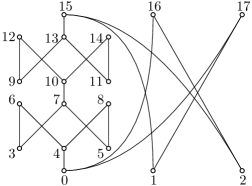
Figure 3: An example for an ordered set that has a transitive incompatibility graph with an inclusion-minimal bipartite subgraph of the transitive incompatibility graph that does not give rise to a two-dimension extension.

(5,9), (3,13), (6,15), (17,15), (5,15), (5,13), (11,10), (9,6), (5,6),
 (4,15), (1,8), (3,15), (11,12), (2,8), (11,7), (0,15), (1,16),

the transitive incomparability graph of this ordered set becomes bipartite. However, if we once again compute the transitive incomparability graph of the new ordered set, we see that it is not bipartite, i.e., the new ordered set is once again not two-dimensional. We have to add the additional pair (17,8) to make the graph two-dimensional. It may be remarked at this point that it is in fact possible to make the transitive incomparability graph bipartite by adding only eleven pairs (in contrast to the seventeen added in this particular example), see Figure 6. Those pairs give rise to a two-dimension extension.

6 Algorithm

Building up on the ideas and notions from the previous sections we propose the Algorithm DimDraw as depicted in Algorithm 1. Given an ordered set $(X,{\leq})$, one calls Compute_Coordinates. Until this procedure identifies a conjugate order using the Comupte_Conjugate_Order (and in turn the algorithm of Golumbic [11]), it computes bipartite subgraphs of the transitive incompatibility graphs. Furthermore it adds the so-computed pairs to the $\leq$. For finite ground sets the algorithm terminates after finitely many steps.

Algorithm 1 DimDraw

Execute Compute_Coordinates on the ordered set that is to be drawn.  

⬇

Input: Ordered set ($P$,$\leq$)

Output: Conjugate order of ($P$,$\leq$)

def Compute_Conjugate_Order($P$,$\leq$):

$C$ $\coloneqq$ Cocomparability_Graph($P$,$\leq$)

if Has_Transitive_Orientation($C$):

($P$,$\leq_{C}$) $\coloneqq$ Transitive_Orientation($C$)

return $\leq_{C}$

else:

return $\perp$

 

⬇

Input: Ordered set ($P$,$\leq$)

Output: Coordinates of the drawing of ($P$,$\leq$)

def Compute_Coordinates($P,\leq$):

$\leq_{C}$ $\coloneqq$ Compute_Conjugate_Order($P,\leq)$

$\mathcal{C}$ $\coloneqq$ $\emptyset$

while $\leq_{C}$ $=$ $\perp$:

$I$ $\coloneqq$ Transitive_Incomparability_Graph($P,{\leq}\cup\mathcal{C}$)

$B$ $\coloneqq$ Maximum_Bipartite_Subgraph($I$)

$\mathcal{C}$ $=$ $\mathcal{C}\cup V(I\backslash B)^{-1}$

$\leq_{C}$ $\coloneqq$ Compute_Conjugate_Order($P$,${\leq}\cup\mathcal{C}$)

$\leq_{1}$ $\coloneqq$ ${\leq}\cup{\leq_{C}}$

$\leq_{2}$ $\coloneqq$ ${\leq}\cup{\geq_{C}}$

for $x$ in $P$:

Coord($x$,1) $\coloneqq$ $|\{k\mid k\leq_{1}x\}|-1$

Coord($x$,2) $\coloneqq$ $|\{k\mid k\leq_{2}x\}|-1$

return Coord

6.1 Postprocessing

The algorithm does not prevent a point from being placed on top of lines connecting two different points. This however is not allowed in order diagrams. Possible strategies to deal with this problem are the following. One strategy is to modify the coordinate system, such that the marks of different integers are not equidistant. Another one is to perturb the points on lines slightly. A third way is to use splines for drawing the line in order to avoid crossing the point.

7 Finding large induced bipartite subgraphs

Our algorithm has to compute an inclusion-minimal set of vertices, such that removing those vertices from the transitive incompatibility graph results in a bipartite graph. Deciding for a graph whether it is possible to make it bipartite by removing a set of cardinality $k$ is known to be $\mathcal{NP}$-complete [15]. Even approximations are known to be in this complexity class [16]. Therefore we propose different approaches.

7.1 Exact solution using a reduction to SAT

Even for small example, i.e., orders on less than 30 elements, a naive approach is infeasible. As we will see in Section 8 the question for computing $\mathcal{C}$ results in $\binom{182}{5}$ tests for an example on $19$ elements (Figure 4) and $\binom{294}{29}$ tests for example (Figure 5) on 24 elements. Therefore we need a more sophisticated solution for the problem. We reduce the problem for finding biparite subgraphs to a SAT problem and then solve this problem with a SAT-Solver, in our case MiniSat [7] in version 2.2. In other words we want to know for some graph $G=(V,E)$ on $n$ vertices and $m$ edges whether by deleting $k$ vertices we can make the graph bipartite. Solving is done by finding a partition of $V$ into the three sets $P_{1},P_{2},\mathcal{C}^{-1}$, such that $P_{1}$ and $P_{2}$ are independent sets and $|\mathcal{C}^{-1}|\leq k$. For this we construct a conjugative normal form as follows: for each vertex $v_{i}$ we have three variables, call them $V_{i,1},V_{i,2},V_{i,3}$. The first two variables indicate, whether the vertex is placed in $P_{1}$ or $P_{2}$, respectively and the third variable indicates, whether the vertex is placed in $\mathcal{C}^{-1}$. For each vertex we have to guarantees, that it is placed in at least one of $P_{1}$, $P_{2}$ or $\mathcal{C}^{-1}$, i.e., at least one of $V_{i,1},V_{i,2},V_{i,3}$ is true for each $i$. We achieve this with the clause $V_{i,1}\vee V_{i,2}\vee V_{i,3}$ for all $i\in\{1,\ldots,n\}$. Also we want to guarantee that $P_{1}$ and $P_{2}$ are independent sets, i.e., no two vertices in $P_{1}$ or $P_{2}$ are connected by an edge. We achive this by adding the two clauses $\neg V_{i,1}\vee\neg V_{j,1}$ and $\neg V_{i,2}\vee\neg V_{j,2}$ for each edge $\{v_{i},v_{j}\}\in E$. This ensures that no two vertices connected by an edge are placed in set $P_{1}$ or $P_{2}$. Finally we have to guarantee, that there are at most $k$ vertices in $P_{3}$, i.e., that at most $k$ of the variables $\{V_{1,3},V_{2,3},\ldots,V_{n,3}\}$ are true. There are multiple ways to achieve this. We employ the method as described in [20]. This results in an additional $(n-1)\cdot k$ auxiliary variables and $2nk+n-3k-1$ clauses. Altogether our SAT instance has in total $(n-1)(k+3)+3$ variables and $2m+2nk+2n-3k-1$ clauses. For this CNF the following holds by construction.

Theorem 7.1

The SAT instance as constructed above is satisfiable if and only if $G$ has an induced bipartite subgraph on $n-k$ vertices.

Now we build this SAT instance for $k$ increasing from 1 until it is satisfiable. Then the set $\{v_{i}\mid V_{i,3}=\text{true}\}$ is exactly the subset of vertices we have to remove to make the graph bipartite. Obviously methods like binary search may be applied here. Furthermore, we may also plug heuristic procedures into our algorithm to find an inclusion-minimal set $\mathcal{C}$. We experimented on this with a greedy algorithm, a simulated annealing approach and a genetic algorithm with promising results, especially for the genetic algorithm. However, it is preferred to use the SAT algorithm as long as there is enough computational power and the problem instances are not too large.

8 Experimental evaluation

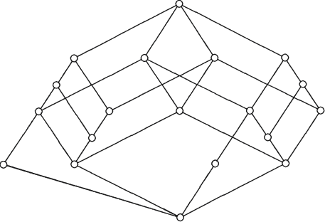
Figure 4: Two drawings of the “Living Beings and Water” lattice, by hand (left) and with our algorithm (right).

Figure 5: The “Drive concepts for motorcars” lattice. Drawn by an expert (left) and two drawings of our algorithm (middle and right).

The DimDraw algorithm was originally designed with the idea in mind to draw the order diagram of lattices. Those are employed in a particular in Formal Concept Analysis (FCA), a mathematical theory for analyzing data. Note that any complete lattice can be represented by a concept lattice in FCA. We tested our algorithm on all lattice examples from a standard literature book on FCA [10]. In all those cases the quality of the produced drawings came close to examples hand drawn by experts. For example, consider the lattice that arises from “Living Beings and Water” [10, p.18]. In Figure 4 we compare the hand-drawn example (left) to the result drawn by our algorithm (right). For Figure 5 [10, p.40] there are two different solutions depicted, both having the minimal number of pairs inserted, note that the algorithm stops after it finds a single solution.

Because of the importance of drawings in FCA we tested the algorithm on every lattice with eleven or less vertices. The reader might want to have a look at the document containing all 44994 drawings on 7499 pages [4].

Concluding the experiments we want to present an example that our algorithm also works on non-lattices. Consider the ordered set from Figure 3. While the hand-drawn version of this order diagram makes use of splines, our algorithm-generated version Figure 6 uses exclusively straight lines.

An interesting observation during the experiments was the following: for all examples of that we are aware, even including those not presented in this work, one pass of the SAT solver was sufficient for reducing the order dimension to two. This is surprising, in particular in light of Figure 3 from Section 5.2.

Figure 6: A non-lattice example drawing produced by the algorithm. See Figure 3 for a hand-drawn version.

9 Conclusion and Outlook

We presented in this work a novel approach for drawing diagrams of order relations. To this end we employed an idea by Doignon et al. relating order dimension and bipartiteness of graphs and proved an extension. Furthermore, we linked the naturally emerging problem to SAT. Finally, we demonstrated various drawings in an experimental evaluation. The drawings produced by the algorithm were, in our opinion, satisfying. We would have liked to compare our algorithm (exact and heuristic type) to the heuristics developed in [14]. Unfortunately, we were not able to reproduce their results based on the provided description.

A notable observation is the fact that in all our experiments the SAT-Solver blend of DimDraw was able to produce a solution in the first pass, i.e., the algorithm found a truly minimal two-dimension extension. This raises the natural question, whether the maximal induced bipartite subgraph approach does always result in a minimal two-dimension extension. Further open questions are concerned with employing heuristics and to improve the postprocessing stage. The SAT-solver version of DimDraw is included in the software conexp-clj. At a later time we also want to include heuristic versions.

Acknowledgement

The authors would like to thank Torsten Ueckerdt for pointing out the research about diametral pairs and Maximilian Stubbemann for helpful discussions.

Appendix 0.A Additional Drawings

In this section we provide some additional drawings generated by DimDraw.

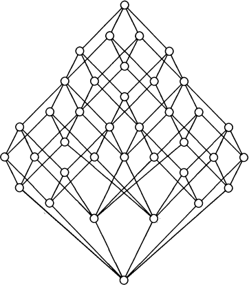
Figure 7: An example from [10, p.53]. The hand-drawn version is on the left, the algorithm-generated version on the right.

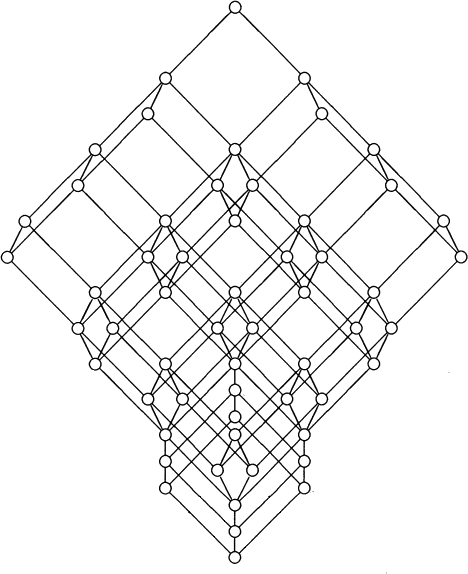
Figure 8: An example from [10, p.35]. The hand-drawn version is on the left, the algorithm-generated version on the right.

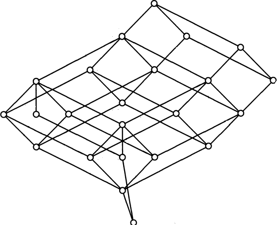
Figure 9: An example from [10, p.30]. The hand-drawn version is on the left, the algorithm-generated version on the right.

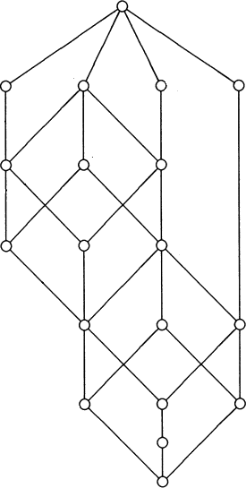
Figure 10: An example from [10, p.45]. The hand-drawn version is on the left, the algorithm-generated version on the right.

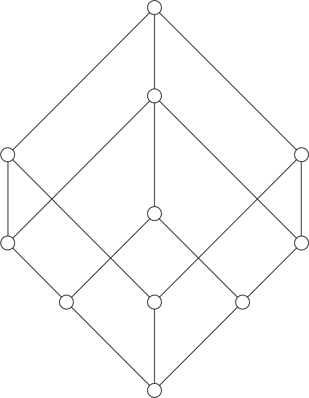
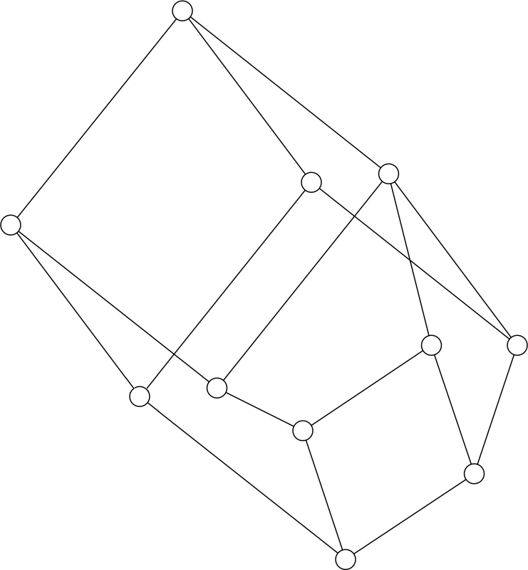
Figure 11: Order diagram of the lattice used in [9]. From left to right: Hand drawn, Ganter’s algorithm, our algorithm.

Figure 12: Order diagrams for boolean lattices of dimension 2, 3, 4 and 5 drawn by our algorithm

References

- [1] Brightwell, G., Massow, M.: Diametral pairs of linear extensions. SIAM Journal on Discrete Mathematics 27(2), 634–649 (Jan 2013)
- [2] Doignon, J.P., Ducamp, A., Falmagne, J.C.: On realizable biorders and the biorder dimension of a relation. Journal of Mathematical Psychology 28(1), 73–109 (1984)
- [3] Dushnik, B., Miller, E.W.: Partially ordered sets. American journal of mathematics 63(3), 600–610 (1941)
- [4] Dürrschnabel, D., Hanika, T., Stumme, G.: Experimental evaluation of dimdraw (Jun 2019), https://doi.org/10.5281/zenodo.3242627
- [5] Eades, P., Wormald, N.: The Median Heuristic for Drawing 2-layered Networks. Technical report, University of Queensland, Department of Computer Science (1986)
- [6] Eades, P., McKay, B.D., Wormald, N.C.: On an edge crossing problem. In: Proc. 9th Australian Computer Science Conference. vol. 327, p. 334 (1986)
- [7] Eén, N., Sörensson, N.: An extensible sat-solver. In: Giunchiglia, E., Tacchella, A. (eds.) Theory and Applications of Satisfiability Testing. pp. 502–518. Springer Berlin Heidelberg, Berlin, Heidelberg (2004)
- [8] Freese, R.: Automated lattice drawing. In: Eklund, P. (ed.) Concept Lattices, LNCS, vol. 2961, pp. 112–127. Springer, Berlin/Heidelberg (2004)
- [9] Ganter, B.: Conflict avoidance in additive order diagrams. Journal of Universal Computer Science, 10(8), 955–966 (2004)
- [10] Ganter, B., Wille, R.: Formal Concept Analysis: Mathematical Foundations. Springer-Verlag, Berlin (1999)
- [11] Golumbic, M.C.: The complexity of comparability graph recognition and coloring. Computing 18(3), 199–208 (1977)
- [12] Kelly, D., Rival, I.: Planar lattices. Canadian Journal of Mathematics 27(3), 636–665– (1975)
- [13] Kornaropoulos, E.M., Tollis, I.G.: Weak dominance drawings and linear extension diameter. CoRR abs/1108.1439 (2011)
- [14] Kornaropoulos, E.M., Tollis, I.G.: Weak dominance drawings for directed acyclic graphs. In: Didimo, W., Patrignani, M. (eds.) Graph Drawing. Lecture Notes in Computer Science, vol. 7704, pp. 559–560. Springer (2012)
- [15] Lewis, J.M., Yannakakis, M.: The node-deletion problem for hereditary properties is np-complete. Journal of Computer and System Sciences 20(2), 219 – 230 (1980)
- [16] Lund, C., Yannakakis, M.: The approximation of maximum subgraph problems. In: Lingas, A., Karlsson, R., Carlsson, S. (eds.) Automata, Languages and Programming. pp. 40–51. Springer Berlin Heidelberg, Berlin, Heidelberg (1993)
- [17] Mcconnell, R.M.: Linear-time transitive orientation. In: In Proceedings of the Eighth Annual ACM-SIAM Symposium on Discrete Algorithms (1997)
- [18] Messinger, E., Rowe, L.A., Henry, R.R.: A divide-and-conquer algorithm for the automatic layout of large directed graphs. IEEE Trans. Systems, Man, and Cybernetics 21(1), 1/2 (1991)
- [19] Reingold, E.M., Tilford, J.S.: Tidier drawings of trees. IEEE Trans. Software Eng. 7(2), 223–228 (1981)
- [20] Sinz, C.: Towards an optimal cnf encoding of boolean cardinality constraints. In: van Beek, P. (ed.) CP. Lecture Notes in Computer Science, vol. 3709, pp. 827–831. Springer (2005)
- [21] Stumme, G., Wille, R.: A geometrical heuristic for drawing concept lattices. In: Tamassia, R., Tollis, I. (eds.) Graph Drawing. LNCS, vol. 894, pp. 452–459. Springer, Heidelberg (1995)
- [22] Sugiyama, K., Tagawa, S., Toda, M.: Methods for visual understanding of hierarchical system structures. IEEE Transactions on Systems, Man & Cybernetics 11(2), 109–125 (1981)
- [23] Trotter, W.T.: Combinatorics and partially ordered sets: Dimension theory, vol. 6. JHU Press (1992)
- [24] Yannakakis, M.: The complexity of the partial order dimension problem. SIAM Journal on Algebraic Discrete Methods 3(3), 351–358 (1982)