Boundary Conditions for Continuum Simulations of Wall-bounded Kinetic Plasmas

Abstract

Continuum kinetic simulations of plasmas, where the distribution function of the species is directly discretized in phase-space, permits fully kinetic simulations without the statistical noise of particle-in-cell methods. Recent advances in numerical algorithms have made continuum kinetic simulations computationally competitive. This work presents the first continuum kinetic description of high-fidelity wall boundary conditions that utilize the readily available particle distribution function. The boundary condition is realized through a reflection function that can capture a wide range of cases from simple specular reflection to more involved first principles models. Examples with detailed discontinuous Galerkin implementation are provided for secondary electron emission using phenomenological and first-principles quantum-mechanical models. Results presented in this work demonstrate the effect of secondary electron emission on a classical plasma sheath.

1 Introduction

Kinetic models of plasmas are necessary to capture processes that occur at small spatial and temporal scales and depend on the shape of a particle distribution. An example of such a process is collisionless Landau damping where an electromagnetic wave is damped in a plasma resulting in a flattening of the particle distribution around its phase velocity. Kinetic simulations are most commonly performed using particle-in-cell (PIC) methods [2]. However, continuum kinetic methods, which involve a direct discretization of the particle distribution function in phase space, are becoming more popular. Continuum kinetic methods are not affected by statistical noise and, with advances in numerical algorithms, are becoming computationally competitive.

This work presents the first simulations of high-fidelity models for electron emission (SEE) in wall-bounded plasmas using a continuum kinetic method. In wall-bounded plasmas, the formation and dynamics of plasma sheaths is an important consideration to study plasma-material interactions. Plasma sheaths are narrow regions of net space charge that occur where electrons and ions come into contact with a solid surface. The process of sheath formation results from significant differences in electron and ion masses and, consequently, their thermal flows. The faster outflow of electrons gives rise to a potential barrier, which equalizes electron and ion fluxes to the wall [27]. This behaviour can be reproduced in the simplest case by setting the particle distribution function to zero for both species, ions and electrons, at the edge of the domain [8, 10] representing an ideal sink.

Despite the small spatial scales associated with plasma sheaths, they play an important role in particle momentum, energy, and heat transfer and on surface erosion, which can have global effects on the plasma. Furthermore, field-accelerated ions and hot electrons are known to cause emission from the solid surface that can further alter the system. One way to include SEE is a constant gain function [12]; however, this technique does not account for the dynamic role of the incoming distribution on the SEE. In reality, the incident particles can be reflected back, penetrate the material and then be rediffused with lower energy, or the electrons originally in the material can gain energy from the incoming particles and be released into the plasma. Plasma sheaths and SEE can influence material and plasma properties in any device where a surface contacts a plasma such as in plasma thrusters [14], fusion devices [34], dielectric barrier and RF discharges [22], to name a few applications.

While there are many models addressing the SEE, they are often based on complex coupling of different tools and/or a Monte-Carlo technique. In this work, a generalized boundary condition implementation for continuum kinetic methods is defined which directly utilizes the information about the particle distribution functions and enables straightforward implementation of various boundary models. Examples using this boundary condition description are tested on simplified boundary conditions and extended for high-fidelity electron emission boundary conditions using a phenomenological model [15] as well as a first-principles based model [4]. The boundary conditions and infrastructure to incorporate electron emission can be extended for other general boundary conditions allowing for computationally efficient solutions of physics-relevant surface models. The SEE boundary conditions and results described in this work are presented using a discontinuous Galerkin (DG) scheme that is extendable to arbitrarily high order, however, the boundary condition descriptions are independent of the numerical method.

The paper is organized as follows. Following the introduction, a brief descriptions of plasma sheath physics and electron emission are provided in Sec. 2 and Sec. 3 respectively. Section 4 presents the description of a continuum kinetic model and the general boundary conditions. Specific examples showing applications of a phenomenological and first-principles models are in Sec. 5 with implementation details for the discontinuous Galerkin continuum kinetic model in the Gkeyll framework (https://gkeyll.rtfd.org/). Results are presented for the first continuum-kinetic plasma sheath simulations using high-fidelity first-principles SEE boundary conditions.

2 Wall-bounded Plasmas & Plasma Sheaths

Interaction of plasma with a solid surface is typically governed by a narrow region near the wall called a plasma sheath. Inside a sheath, otherwise quasi-neutral plasma has a non-zero space charge. The charge is usually positive but inverse sheaths with negative charge have been predicted in theory [11]. The size of a sheath is typically on the order of tens of Debye lengths with a Debye length defined as,

$$\lambda_{\mathrm{D}}=\sqrt{\frac{\varepsilon_{0}\mathrm{k_{B}}T_{\mathrm{e}}}{n_{\mathrm{e}}q_{\mathrm{e}}^{2}}},$$

where $\varepsilon_{0}$ is vacuum permittivity, $T_{\mathrm{e}}$ is electron temperature in energetic units, $n_{\mathrm{e}}$ is electron number density, and $q_{\mathrm{e}}$ is the electron charge.

Plasma sheaths form near a wall due to discrepancy in masses of plasma species. With comparable temperatures, this difference results in different thermal velocities/fluxes. Electrons, as the lightest species in a plasma, are quickly absorbed into the wall [27]. The charge then gives rise to a potential barrier, which works to equalize fluxes to the wall. Despite the microscopic nature of a sheath, it plays an important role in transfer of particles, momentum, energy, and heat transfer and in surface erosion, all of which can have global effects on the plasma. Furthermore, field-accelerated ions and hot electrons are known to cause an emission from the solid surface that can further alter the system [21].

Formation of a sheath is strongly affected by boundary conditions at the wall, such as electron emission, which is the main topic of this paper. For simplicity, an ideally absorbing wall is considered to describe sheath and plasma behavior. For this simplified model, the domain is divided into a quasi-neutral part where $n_{\mathrm{e}}=n_{\mathrm{i}}=n_{0}$ and the non-neutral sheath with monotonically decreasing potential, $\phi$, [19, 26]. The cold ions are assumed to enter the sheath region with a non-zero velocity $u_{\mathrm{i},0}$ and then ”free-fall” through the potential. The ion density inside the non-neutral region is then obtained from the conservation of mass and energy,

$$n_{\mathrm{i}}(x)=n_{0}\left(1-\frac{2q_{\mathrm{i}}\phi(x)}{m_{\mathrm{i}}u_{\mathrm{i},0}^{2}}\right)^{-\frac{1}{2}}.$$ (1)

Electrons are assumed to instantly follow the electric potential,

$$n_{\mathrm{e}}(x)=n_{0}\exp\left(-\frac{q_{\mathrm{e}}\phi}{\mathrm{k_{B}}T_{\mathrm{e}}}\right).$$ (2)

These densities are substituted into Poisson’s equation,

$$\frac{\partial^{2}\phi(x)}{\partial x^{2}}=-\frac{n_{\mathrm{e}}(x)q_{\mathrm{e}}+n_{\mathrm{i}}(x)q_{\mathrm{i}}}{\varepsilon_{0}}=-\frac{n_{0}}{\varepsilon_{0}}\left[q_{\mathrm{e}}\exp\left(-\frac{q_{\mathrm{e}}\phi}{\mathrm{k_{B}}T_{\mathrm{e}}}\right)+q_{\mathrm{i}}\left(1-\frac{2q_{\mathrm{i}}\phi(x)}{m_{\mathrm{i}}u_{\mathrm{i},0}^{2}}\right)^{-\frac{1}{2}}\right].$$ (3)

Even though this equation cannot be solved analytically to obtain sheath profiles, it leads to the classical Bohm sheath criterion [3],

$$u_{\mathrm{i},0}\geq u_{\mathrm{B}}=\sqrt{\frac{Z\mathrm{k_{B}}T_{\mathrm{e}}}{m_{\mathrm{i}}}},$$ (4)

where $Z$ is ion ionization state. In this work, ions are assumed to be singly ionized but have a non-zero temperature. Therefore, the Bohm velocity used here has a slightly different form [35],

$$u_{\mathrm{i},0}\geq u_{\mathrm{B}}=\sqrt{\frac{\mathrm{k_{B}}T_{\mathrm{e}}+\upgamma\mathrm{k_{B}}T_{\mathrm{i}}}{m_{\mathrm{i}}}},$$ (5)

where $\upgamma$ is the heat capacity ratio, which can be defined through the number of degrees of freedom, $N$, as $\upgamma=(N+2)/N$.

Further physical insight into the Bohm criterion can be obtained from Fig. 1. This figure presents a single electron density profile (blue line) in the non-neutral sheath region together with three ion densities based on $M=u_{0}/u_{\mathrm{B}}$. If the ions are not accelerated to the Bohm velocity in the presheath (red dashed line denoting $M<1$), there is a point inside the sheath where the charge density changes sign which contradicts the original assumption of a monotonic potential drop. This is further emphasized by the red highlighted region in the plot. It is worth noting that this behavior is significantly altered by presence of magnetic fields [20] and by ionization inside the sheath and emission from the wall [11].

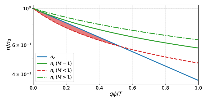
Figure 1: Electron (blue) and ion (green and red) densities inside the non-neutral sheath region as a function of sheath potential for different ion Mach numbers. The ion densities are depicted based on the ratio of the ion velocity at the sheath entrance to the Bohm velocity. When the ions are not accelerated sufficiently in the presheath (red dashed line for $M<1$), the charge density changes sign inside the sheath, thus violating the original assumption as shown by the highlighted region. The figure is adapted from a Ph.D. dissertation [10]

A simplified model for sheath profiles including a uniform volumetric source term, $S$, is described by Robertson [27]. Solutions to this simplified model are presented in Fig. 2 for normalized electron and ion densities, electric field, potential, and ion bulk velocities. Ions, accelerated by the presheath electric field, reach the Bohm velocity around $8\,\lambda_{\mathrm{D}}$ from the wall. The charge non-neutrality becomes visually apparent around the same point as well.

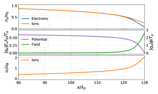
Figure 2: Simulated profiles of electron and ion densities, electric field and potential, and ion drift velocity obtained from a simplified sheath model by Robertson [27]. An ideally absorbing wall is located on the right side of the domain. Ions are accelerated by the presheath electric field and reach the Bohm velocity around $8\,\lambda_{\mathrm{D}}$ from the wall. At the same point, the charge non-neutrality becomes apparent. The figure is adapted from a Ph.D. dissertation [10].

3 Electron Emission from a Wall

The treatment of a wall as an ideal absorber is often an unphysical approximation. In reality, some incoming particles are reflected from the wall and some particles originating in the wall may enter the plasma. The particles originating from the wall need to gain energy to cross the surface potential barrier of the material. One pathway is by direct [15] or indirect [5] energy transfer from the incoming particles. Alternatively, the particles can gain energy by wall heating or incoming electromagnetic radiation.

A common way to quantify the electron emission is through emission yield, $\gamma$, which is defined as a ratio between the outgoing and incoming fluxes. Yields depend on material and incoming particle energy. For example, incoming particles with energy below $600\text{\,}\mathrm{e}\mathrm{V}$ have a maximum yield of 0.56 for lithium, 0.97 for aluminum, and 1.27 for copper [7].

Particle emission from a wall can have significant effects on the sheath and consequently on global plasma behavior. With emission yields above zero, $\gamma>0$, the sheath can reach a space-charge limitation [29, 32, 30]. For $\gamma>1$, there are predictions that sheath potential can reverse entirely [11].

4 General Boundary Conditions for Kinetic Plasmas

The models presented in Section 2 do not properly account for velocity distributions of particles. When the plasma satisfies a Maxwellian distribution, fluid models are often sufficient to describe the dynamics. However, the distribution inside a sheath is non-Maxwellian [33, 18] and fully kinetic models are needed.

A fully kinetic model can be derived from a continuous description of discrete particles,

$$N_{s}(t,\bm{x},\bm{v})=\sum_{i}\delta\big{(}\bm{x}-\bm{X}_{i}(t)\big{)}\delta\big{(}\bm{v}-\bm{V}_{i}(t)\big{)},$$ (6)

where the sum is performed over all the particles of the same species $s$. The vectors $\bm{X}_{i}$ and $\bm{V}_{i}$ are positions and velocities for all the particles $i$. Taking a time derivative of $N$ and substituting the definition of velocity $\bm{\dot{X}}_{i}(t)=\bm{V}_{i}(t)$ and Newton’s second law with the Lorentz force,

$$m_{s}\bm{\dot{V}}_{i}=q_{s}\bm{E}^{m}\big{(}t,\bm{X}_{i}(t)\big{)}+q_{s}\bm{V}_{i}(t)\times\bm{B}^{m}\big{(}t,\bm{X}_{i}(t)\big{)},$$ (7)

leads to the Klimontovich equation [23],

$$\frac{\partial N_{s}(t,\bm{x},\bm{v})}{\partial t}+\bm{v}\cdot\nabla_{\bm{x}}N_{s}+\frac{q_{s}}{m_{s}}\left(\bm{E}^{m}+\bm{v}\times\bm{B}^{m}\right)\cdot\nabla_{\bm{v}}N_{s}=0.$$ (8)

Knowing the electromagnetic field, Eq. (7) fully describes a collection of particles in continuous phase space. However, the density, $N$, is still a sum of Dirac $\delta$-functions. It can be approximated by a smooth function by taking an ensemble average, $f_{s}(\bm{x},\bm{v},t)\mathrel{\mathop{\ordinarycolon}}=\left\langle N_{s}(\bm{x},\bm{v},t)\right\rangle$, [23]. $f$ is referred to as the particle distribution function. The Klimontovich equation (Eq. 8) then transforms into the Boltzmann equation,

$$\frac{\partial f_{s}}{\partial t}+\bm{v}\cdot\nabla_{\bm{x}}f_{s}+\frac{q_{s}}{m_{s}}\left(\bm{E}+\bm{v}\times\bm{B}\right)\cdot\nabla_{\bm{v}}f_{s}=\underbracket{-\frac{q_{s}}{m_{s}}\big{\langle}\left(\delta\bm{E}+\bm{v}\times\delta\bm{B}\right)\cdot\nabla_{\bm{v}}\delta N_{s}\big{\rangle}}_{\sum\left(\frac{\partial f_{s}}{\partial t}\right)_{c}},$$ (9)

where $\delta N_{s}(\bm{x},\bm{v},t)=N_{s}(\bm{x},\bm{v},t)-f_{s}(\bm{x},\bm{v},t)$, etc. The term on the right-hand-side of Eq. (9) corresponds to the intrinsically discrete nature of particles like collisions [28]. When the RHS is zero, the equation is referred to as the Vlasov equation. Note that the individual species, $s$, are evolved separately. They are coupled with electrostatic or electromagnetic fields and aforementioned collisions.

Fig. 3 presents the distribution functions for ions and electrons constructed from the density and momentum in Fig. 2 assuming a Maxwellian distribution with constant temperature across the domain. The green line in the bottom panel marks the bulk velocity of the ions and the dashed white line represents the Bohm speed. Note that the point where the ion bulk velocity reaches the Bohm speed is consistent with Fig. 2.

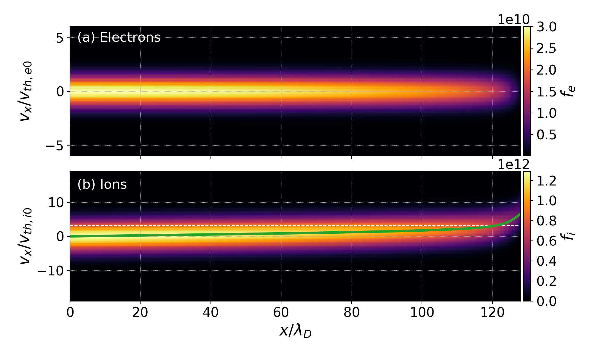
Figure 3: Electron (top) and ion (bottom) distribution functions constructed from the density and momentum presented in Fig. 2. An absorbing wall is on the right side of the domain. The green line in the bottom panel marks the bulk velocity of the ions and the dashed white line represents the Bohm speed.

As shown in previous work [8], classical sheath results using ideally absorbing walls as boundaries (mentioned in Section 2) can be reproduced by setting the outgoing distribution to zero at the wall, $f_{\mathrm{out}}(t,\,\bm{x}=\bm{x}_{\mathrm{wall}},\,\bm{v})=0$. These results also confirm, that the electron distribution function near the wall is not Maxwellian. Furthermore, the availability of full particle distribution functions, which are not contaminated by statistical noise, near a wall can be used for more complex boundary conditions when the particles are not simply absorbed.

Following is a general formulation of a boundary condition for a distribution function near a wall assuming the entire incoming (incoming implies to the wall) distribution function is known. The definition also includes a source term for effects like thermionic emission which are not directly functions of the incoming distribution but rather parameters of the wall, e.g., its temperature. These terms will be addressed in future work.

Definition 1.

Distribution function of particles coming out of a wall, $f_{\mathrm{out}}$, is given by the incoming distribution function, $f_{\mathrm{in}}$ and a reflection function, $R$,

$$f_{\mathrm{out}}(t,\,\bm{x}=\bm{x}_{\mathrm{wall}},\,\bm{v})=\iiint_{\mathcal{V}_{\mathrm{in}}}R(\bm{v},\,\bm{v}^{\prime})f_{\mathrm{in}}(t,\,\bm{x}^{\prime}=\bm{x}_{\mathrm{wall}},\,\bm{v}^{\prime})\,\operatorname{d\!}\bm{v}^{\prime}+f_{\mathrm{source}}(T_{\mathrm{wall}},...),\quad\forall\bm{v}\in\mathcal{V}_{\mathrm{out}}$$ (10)

where the integration is performed over the velocities coming to the wall, $\bm{v}\in\mathcal{V}_{\mathrm{in}}$. $f_{\mathrm{source}}$ is a source term including effects like thermionic emission, which are generally functions of the wall conditions.

Usage of this boundary condition can be demonstrated on specular reflection. Without loss of generality, the wall is assumed perpendicular to the $x$-direction. The reflection function is then defined using Dirac $\delta$-functions,

$$R_{\mathrm{x}}(\bm{v},\bm{v}^{\prime})=\delta(v_{\mathrm{x}}+v_{\mathrm{x}}^{\prime})\delta(v_{\mathrm{y}}-v_{\mathrm{y}}^{\prime})\delta(v_{\mathrm{z}}-v_{\mathrm{z}}^{\prime}).$$ (11)

For this reflection function, the integral Eq. (10) can be calculated analytically and the boundary condition gives the expected result,

$$f_{\text{out}}(v_{\mathrm{x}},v_{\mathrm{y}},v_{\mathrm{z}}) =\iiint_{\mathcal{V}_{\text{in}}}\delta(v_{\mathrm{x}}+v_{\mathrm{x}}^{\prime})\delta(v_{\mathrm{y}}-v_{\mathrm{y}}^{\prime})\delta(v_{\mathrm{z}}-v_{\mathrm{z}}^{\prime})f_{\text{in}}(v_{\mathrm{x}}^{\prime},v_{\mathrm{y}}^{\prime},v_{\mathrm{z}}^{\prime})\,\operatorname{d\!}v_{\mathrm{x}}^{\prime}\operatorname{d\!}v_{\mathrm{y}}^{\prime}\operatorname{d\!}v_{\mathrm{z}}^{\prime},$$

$$=f_{\text{in}}(-v_{\mathrm{x}},v_{\mathrm{y}},v_{\mathrm{z}}).$$

This example is included here to demonstrate the approach. The reflection function, $R$, can be replaced by more complex models using the same framework. Presented below are two special cases of a reflection function for electron emission using a phenomenological model and a first-principles quantum mechanical model.

Electron Emission Boundary Condition: Furman & Pivi (2002) model

Furman & Pivi [15] describe a widely used and referenced phenomenological model, which uses analytical descriptions for three populations of electron emission – elastically reflected electrons, rediffused electrons, and true-secondary electrons. These species are assumed to be produced by a mono-energetic (cold) beam of incoming electrons. For each incident beam with current $I_{\text{in}}$, the model defines energetic distribution of electron yield, $\gamma=I_{\text{out}}/I_{\text{in}}$,

$$\frac{\partial\gamma}{\partial E}=\frac{\partial\gamma_{\mathrm{e}}}{\partial E}+\frac{\partial\gamma_{\mathrm{r}}}{\partial E}+\frac{\partial\gamma_{\mathrm{ts}}}{\partial E},$$ (12)

where $\gamma_{\mathrm{e}}$, $\gamma_{\mathrm{r}}$, and $\gamma_{\mathrm{ts}}$ correspond to the three aforementioned populations. An analytical profile for each population is determined based on underlining physical properties and experimental data.

The first described group consists of primary electrons semi-elastically reflected from the material surface. Since they are assumed not to lose any energy or only a small amount, the model approximates this population with a narrow half-Gaussian centered around the incoming energy. Note that since the secondary electrons cannot have higher energy than the incident ones (unless additional energy is provided, for example, by heating), the distribution is cropped at the incoming energy. The contribution of the reflected electrons is given as,

$$\frac{\partial\gamma_{\mathrm{e}}}{\partial E}(E,E^{\prime}\mu^{\prime})=\theta(E)\theta(E^{\prime}-E)\,\gamma_{\mathrm{e}0}(E^{\prime})\left[1+e_{1}\left(1-\mu^{\prime e_{2}}\right)\right]\frac{2\exp\big{(}-(E-E^{\prime})^{2}/2\sigma_{\mathrm{e}}^{2}\big{)}}{\sqrt{2\pi}\sigma_{\mathrm{e}}\mathrm{erf}\left(E^{\prime}/\sqrt{2}\sigma_{\mathrm{e}}\right)},$$ (13)

$$\gamma_{\mathrm{e}0}(E^{\prime})=P_{1,\mathrm{e}}(\infty)+\left[\hat{P}_{1,\mathrm{e}}-P_{1,\mathrm{e}}(\infty)\right]\exp\left[\left(|E^{\prime}-\hat{E}_{\mathrm{e}}|/W\right)^{p}/p\right],$$

where $\theta(\cdot)$ is the Heaviside step function ensuring that the incoming energy is higher than the outgoing. $e_{1}$, $e_{2}$, $\sigma_{e}$, $P_{1,\mathrm{e}}(\infty)$, $\hat{P}_{1,\mathrm{e}}$, $W$, $\hat{E}_{\mathrm{e}}$, and $p$ are fitting parameters. $\mu$ and $\mu^{\prime}$ are direction cosines for the outgoing and incoming angles, respectively.

The rest of the incident electrons are assumed to penetrate the material. As they interact with the material, they lose energy. A part of them eventually penetrate through the material potential barrier again and return to the plasma. These rediffused electrons can have a wide range of energies between zero and the incident energy,

$$\frac{\partial\gamma_{\mathrm{r}}}{\partial E}(E,E,\mu^{\prime})=\theta(E)\theta(E^{\prime}-E)\gamma_{\mathrm{r}0}(E^{\prime})\left[1+r_{1}\left(1-\mu^{\prime r_{2}}\right)\right]\frac{(q+1)E^{q}}{E^{\prime q+1}},$$ (14)

$$\gamma_{\mathrm{r}0}(E^{\prime})=P_{1,\mathrm{r}}(\infty)\left[1-\exp\big{(}-(E^{\prime}/E_{\mathrm{r}})^{r}\big{)}\right],$$

where $r$, $r_{1}$, $r_{2}$, $q$, $P_{1,\mathrm{r}}(\infty)$, and $E_{\mathrm{r}}$ are fitting constants.

The third group consists of the true-secondary electrons from the material. Since the energy of the primary beam is transferred to the secondary electrons through a cascade, their distribution peaks at lower energy. However, unlike the back-scattered and rediffused electrons, a single incoming electron can produce multiple secondaries. As a result, the contribution of the true secondary electrons is more involved compared to the other populations and is

$$\frac{\partial\gamma_{\mathrm{ts}}}{\partial E}(E,E,\mu^{\prime})=\sum_{n=1}^{M}\frac{nP_{n,\mathrm{ts}}(E^{\prime},\mu^{\prime})(E/\epsilon_{n})^{p_{n}-1}\exp(-E/\epsilon_{n})}{\epsilon_{n}\Gamma(p_{n})P(np_{n},E^{\prime}/\epsilon_{n})}P\big{(}(n-1)p_{n},(E^{\prime}-E)\epsilon_{n}\big{)},$$ (15)

$$P_{n,\mathrm{ts}}(E^{\prime},\mu^{\prime})=\binom{M}{n}\left(\frac{\hat{\gamma}(\mu^{\prime})D\left[E^{\prime}/\hat{E}(\mu^{\prime})\right]}{M}\right)^{n}\left(1-\frac{\hat{\gamma}(\mu^{\prime})D\left[E^{\prime}/\hat{E}(\mu^{\prime})\right]}{M}\right)^{M-n},$$

$$\hat{\gamma}(\mu^{\prime})=\hat{\gamma}_{\mathrm{ts}}\left[1+t_{1}\left(1-\mu^{\prime t_{2}}\right)\right],\quad\hat{E}(\mu^{\prime})=\hat{E}_{\mathrm{ts}}\left[1+t_{3}\left(1-\mu^{\prime t_{4}}\right)\right],$$

$$D(x)=\frac{sx}{s-1+x^{s}},$$

where $t_{1}$, $t_{2}$, $t_{3}$, $t_{4}$, $p_{n}$, $\epsilon_{n}$, $\hat{\gamma}_{\mathrm{ts}}$, $\hat{E}_{\mathrm{ts}}$ and $s$ are fitting variables. $\Gamma(\cdot)$ is the gamma function and $P(\cdot,\cdot)$ is the normalized incomplete gamma function. Note that the summation in Eq. (15) should theoretically go to infinity, but error from limiting it to $M=10$ is negligible [15].

An example of secondary electron distributions emitted by a single $200\text{\,}\mathrm{e}\mathrm{V}$ electron beam calculated from Eq. (13), Eq. (14), and Eq. (15) using parameters from Tab. I and Tab. II of Ref. [15] are in Fig. 4. Integrating the area under the curves of individual populations yields the total gains $\gamma_{\mathrm{e}}=0.1241$ for back-scattered electrons, $\gamma_{\mathrm{r}}=0.7350$ for rediffused, and $\gamma_{\mathrm{ts}}=1.1283$ for true-secondary electrons for stainless steel. Note that $\gamma_{\mathrm{e}}+\gamma_{\mathrm{r}}<1$ is required but, for this case, $\gamma_{\mathrm{ts}}>1$. Note that even though more particles are returned to the system, their total kinetic energy is lower than the energy of the incoming beam.

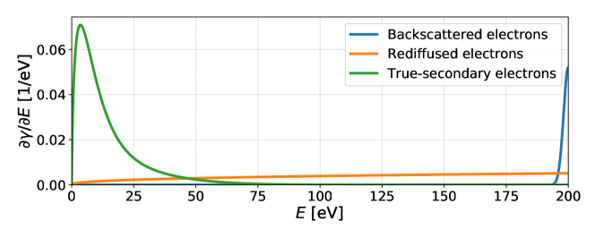
Figure 4: The energetic distribution of the three particle populations emitted by a single $200\text{\,}\mathrm{e}\mathrm{V}$ electron mono-energetic beam with normal incidence for stainless steel based on the phenomenological model fits [15]. Figure taken from a Ph.D dissertation [10].

The gain, $\partial\gamma/\partial E$, is required as an intermediate step to obtain emission probabilities for Monte-Carlo SEE codes. However, $\partial\gamma/\partial E^{\prime}(E,E^{\prime},\mu)$ resembles the reflection function in Eq. (10) since

$$\int_{0}^{\infty}\frac{\partial\gamma}{\partial E}\,\operatorname{d\!}E=\gamma(E^{\prime}).$$

The dependence on the outgoing angle is the only missing part. Experimental measurements show that the dependence is a cosine function for the true-secondary electrons [6], i.e., the incoming and outgoing angles are completely uncorrelated. While this is not quite true for the other two populations, Furman & Pivi [15] make this assumption as well. In other words, this model can be directly used as a reflection function, $R$, in Eq. (10),

$$f_{\text{out}}(E,\mu)=\int_{0}^{1}\int_{0}^{\infty}\mu\frac{\partial\gamma}{\partial E}(E,E^{\prime},\mu^{\prime})f_{\text{in}}(E^{\prime},\mu^{\prime})\,\operatorname{d\!}E^{\prime}\operatorname{d\!}\mu^{\prime}.$$

The integral can be seen as a “summation” over all incoming cold beams in order to extend the mono-energetic formulation for thermal populations. Finally, the expression needs to be correctly transformed from energetic units, typical for surface physics, to phase space velocity coordinates. Noting that

$$\frac{\partial\gamma}{\partial v_{\mathrm{x}}}=\frac{\partial\gamma}{\partial E}\frac{\partial E}{\partial v_{\mathrm{x}}}=\frac{\partial\gamma}{\partial E}mv_{\mathrm{x}},$$

the boundary condition 1D ($\mu\equiv 1$) becomes

$$f_{\text{out}}(v_{\mathrm{x}})=\int\mu(v_{\mathrm{x}})\frac{\partial\gamma}{\partial E}\big{(}E(v_{\mathrm{x}}),E(v_{\mathrm{x}}^{\prime}),\mu(v_{\mathrm{x}}^{\prime})\big{)}mv_{\mathrm{x}}f_{\text{in}}(v_{\mathrm{x}}^{\prime})\,\operatorname{d\!}v_{\mathrm{x}}^{\prime}.$$ (16)

The behavior of this reflection function can be tested on a synthetic Maxwellian distribution function. Fig. 5 presents the results with colors of the populations corresponding to those in Fig. 4. Note that the reflected electrons have the largest population when using a distribution, even though their gain in Fig. 4 is the smallest. Fig. 4 depicts a case where incoming particles have enough energy to penetrate the material, limiting the contribution of the back-scattered electrons. As the energy decreases, the back-scattered electrons become the dominant species. This is the case for electron populations with temperatures on the order of an electron volt with bulk velocity comparable to thermal velocity.

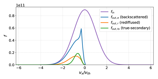
Figure 5: Application of the reflection function from [15] on a Maxwellian distribution function. The violet line represents a simulated incoming distribution function at the right wall boundary and blue, orange, and green are distributions of the reflected populations (colors correspond to Fig. 4). Figure taken from a Ph.D. dissertation [10].

Fig. 6 provides further insight into the individual secondary populations based on the incoming beam energy. It extends Fig. 4 to include multiple incoming beam energies, i.e., the $y$-axis of Fig. 6 corresponds to $x$-axis of Fig. 4. However, since the outgoing energies are limited by the incoming energy, the $y$-axis of Fig. 6 is normalized to the incoming energy for better visualization. Analogously, the values of $\partial\gamma/\partial E$ are multiplied by $E^{\prime}$ to allow for comparison of magnitudes. This reveals a gradually decreasing relative contribution of the true-secondary emission, while the rediffused electron contribution remains approximately constant for a larger range of energies prior to decreasing for $E^{\prime}<$20\text{\,}\mathrm{e}\mathrm{V}$$. On the other hand, as the incoming energy decreases, the backscattered electron population becomes more significant which is consistent with results in Fig. 5.

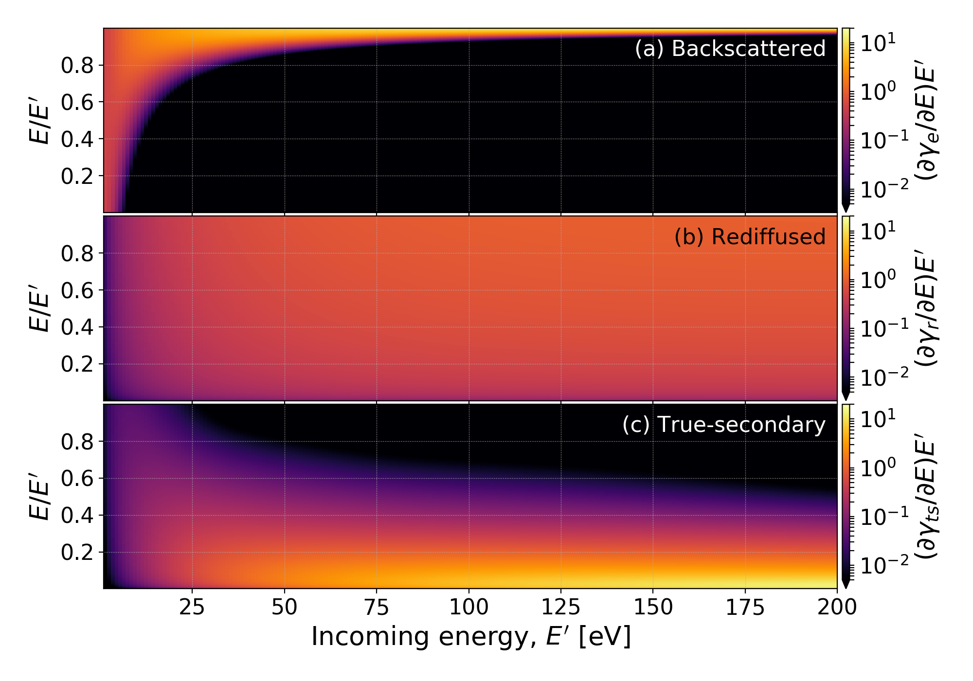
Figure 6: Contributions of the secondary populations from the phenomenological model [15], based on the incoming energy. Both the values and the $y$-axis are normalized to the incoming energy to allow for better comparison of the relative contributions. From top to bottom the figure captures backscattered (elastically reflected) electrons, rediffused electrons, and true-secondary electrons. Figure taken from a Ph.D. dissertation [10].

Furthermore, note that although the model is mathematically sound for incoming energies all the way to zero, the values at the lower energy range, which are crucial as described above, are from an extrapolation of higher energy beam data. Therefore, for simulating $\sim$10\text{\,}\mathrm{e}\mathrm{V}$$ electron distributions in contact with a wall, a different model specifically tailored for these energies might be preferred. Another disadvantage of the model is its dependency on a significant number of fitting parameters which do not necessarily correspond to physical quantities. This limits the materials that this model extends to.

Electron Emission Boundary Condition: Bronold & Fehske (2015) model

Bronold & Fehske [4] present a model for electron absorption by a dielectric wall, which is based on first principles from quantum mechanics. In comparison to the previous model, it has fewer fitting parameters and most of them have physical relevance. As a result, it is applicable to a wide range of materials based on standard physical parameters that can be obtained from material databases. The disadvantage of this model is that it is accurate only up to incoming energies comparable to the electron band gap $E_{\mathrm{g}}\sim$10\text{\,}\mathrm{e}\mathrm{V}$$ ($E_{\mathrm{g}}=$7.8\text{\,}\mathrm{e}\mathrm{V}$$ for MgO used for examples here).

Here, the reflection function is defined directly,

$$R(E,\mu,E^{\prime},\mu^{\prime})=\underbracket{R(E^{\prime},\mu^{\prime})\delta(E-E^{\prime})\delta(\mu-\mu^{\prime})}_{\text{backscattered}}+\underbracket{\delta R(E,\mu,E^{\prime},\mu^{\prime})}_{\text{rediffused}}.$$ (17)

Note that the model assumes specular reflection for the back-scattered electrons, i.e., the energy and angles are conserved with variable probability $R(E^{\prime},\mu^{\prime})$, which is a function only of the incoming properties. It is given as $R(E^{\prime},\mu^{\prime})=1-\mathcal{T}(E^{\prime},\mu^{\prime})$, where $\mathcal{T}(E^{\prime},\mu^{\prime})$ is the probability of a quantum-mechanical reflection,

$$\mathcal{T}(E^{\prime},\mu^{\prime})=\frac{4\overline{m}_{\mathrm{e}}kp}{(\overline{m}_{\mathrm{e}}k+p)^{2}},\quad k=\sqrt{E^{\prime}-\chi}\mu^{\prime},\quad p=\sqrt{\overline{m}_{\mathrm{e}}E^{\prime}}\nu^{\prime}.$$

$\overline{m}_{\mathrm{e}}$ is the relative mass of a conduction band electron and $\chi$ is the electron affinity of the dielectric. $k$ and $p$ are components of momentum perpendicular to the wall where $\nu$ is the cosine angle inside the wall. $\nu$ is connected with $\mu$ through conservation of energy and lateral momentum,

$$1-\nu^{\prime 2}=\frac{E^{\prime}-\chi}{\overline{m}_{\mathrm{e}}E^{\prime}}(1-\mu^{\prime 2}).$$ (18)

The probability of reflection, $R(E^{\prime},\mu^{\prime})$ is captured in Fig. 7. Note the region of $R(E^{\prime},\mu^{\prime})=1$ for $E^{\prime}<$1\text{\,}\mathrm{e}\mathrm{V}$$. This region contains electrons with energy below the affinity of the material. These electrons cannot penetrate the potential barrier and are all reflected. As a direct consequence of the conservation of energy and lateral momentum (Eq. 18), there is a critical angle given as $\mu_{\mathrm{c}}=\sqrt{1-\overline{m}_{\mathrm{e}}E^{\prime}/(E^{\prime}-\chi)}$. Particles entering under this angle have the momentum vector perpendicular to the surface after penetrating the material; particles that hit the wall with $\mu^{\prime}<\mu_{\mathrm{c}}$ are reflected. Note that particles with $\mu^{\prime}>\mu_{\mathrm{c}}$ and $E^{\prime}>$2\text{\,}\mathrm{e}\mathrm{V}$$ generally do penetrate the material and would be lost from the plasma if back-scattering was the only effect taken into account. They can, however, return to the plasma through rediffusion.

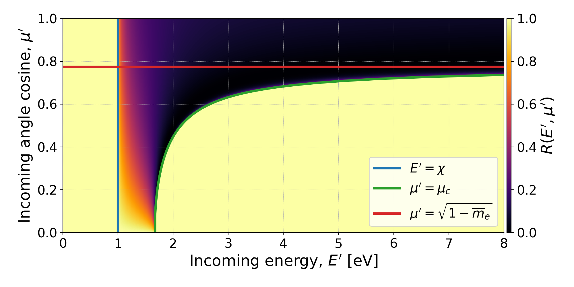
Figure 7: Probability of back-scattering, $R(E^{\prime},\mu^{\prime})$, from the quantum mechanics based model [4] as a function of incoming angle and energy. Highlighted are $E^{\prime}=\chi$ (blue line) below which all particles are reflected, and the critical angle $\mu_{\mathrm{c}}$ (green line) given by the conservation laws, (Eq. 18). The red line marks the angle above which rediffusion is possible, (Eq. 19). Used parameters are for MgO, $\chi=$1\text{\,}\mathrm{e}\mathrm{V}$$ and $\overline{m}_{\mathrm{e}}=0.4$. Figure adapted from a Ph.D. dissertation [10].

Description of rediffusion is more involved in comparison to back-scattered electrons [5],

$$\delta R(E,\mu,E^{\prime},\mu^{\prime})=\frac{\partial\nu}{\partial\mu}\mathcal{T}(E^{\prime},\mu^{\prime})\rho(E)\mathcal{B}(E,\mu,E^{\prime},\mu^{\prime})\mathcal{T}(E,\mu)\theta\big{(}\mu-\sqrt{1-\overline{m}_{\mathrm{e}}}\big{)},$$ (19)

where $\rho(E)=\sqrt{\overline{m}_{\mathrm{e}}^{3}E}/2(2\pi)^{3}$ is the conduction band density of states and

$$\mathcal{B}(E,\mu,E^{\prime},\mu^{\prime})=\frac{Q(E,\mu,E^{\prime},\mu^{\prime})}{\int_{0}^{1}\int_{0}^{E^{\prime}}\rho(E)Q(E,\mu,E^{\prime},\mu^{\prime})\,\operatorname{d\!}E\operatorname{d\!}\mu}$$

is the probability of rediffusion. $Q(E,\mu,E^{\prime},\mu^{\prime})$ is given by a recursive relation summed over the back-scattering events inside the material. Note the Heaviside step function in Eq. (19); the limiting $\mu$ is marked by the blue line in Fig. 7. The population with cosine angles above this line can return to the domain after penetrating the material, significantly influencing Eq. (17). True-secondary electrons excited by incoming electrons with energies considered here ($<$10\text{\,}\mathrm{e}\mathrm{V}$$) are neglected in this model.

This model can be implemented into the simulation in the same manner as the previous phenomenological model [15]. All the relations above are derived for ideally flat walls without any defects. To address effects of real walls, the authors modify the relations by adding a roughness parameter $C$ [31], which is proportional to the density scattering centers. With $C=1$ and $C=2$ the results match experimental data very well (see Fig. 3 in [4]; results are much better than for $C=0$). Furthermore, with increasing $C$, the effects of $\delta R(E,\mu,E^{\prime},\mu^{\prime})$ become less important. This presents an opportunity to develop reasonably accurate and computational inexpensive boundary conditions by neglecting the rediffusion and using the roughness-modified formula for the probability of a quantum-mechanical reflection (Eq. (13) in [4]),

$$\overline{\mathcal{T}}(E^{\prime},\mu^{\prime})=\frac{\mathcal{T}(E^{\prime},\mu^{\prime})}{1+C/\mu^{\prime}}-\frac{C/\mu^{\prime}}{1+C/\mu^{\prime}}\int_{\mu_{\mathrm{c}}}^{1}\mathcal{T}(E^{\prime},\mu^{\prime\prime})\,\operatorname{d\!}\mu^{\prime\prime}.$$ (20)

Calculating these integrals for the reflection function of each particle would still be quite expensive. However, as emphasized before, the energies and angles need to be treated as coordinates and the integrals can be precomputed substantially decreasing computational cost.

The reflection function, $R$, calculated with $\overline{\mathcal{T}}$ then significantly alters Fig. 7. The modified version is in Fig. 8. Particularly noticeable is the absence of regions with absolute reflection in the bottom-right sector (higher energies and oblique angles).

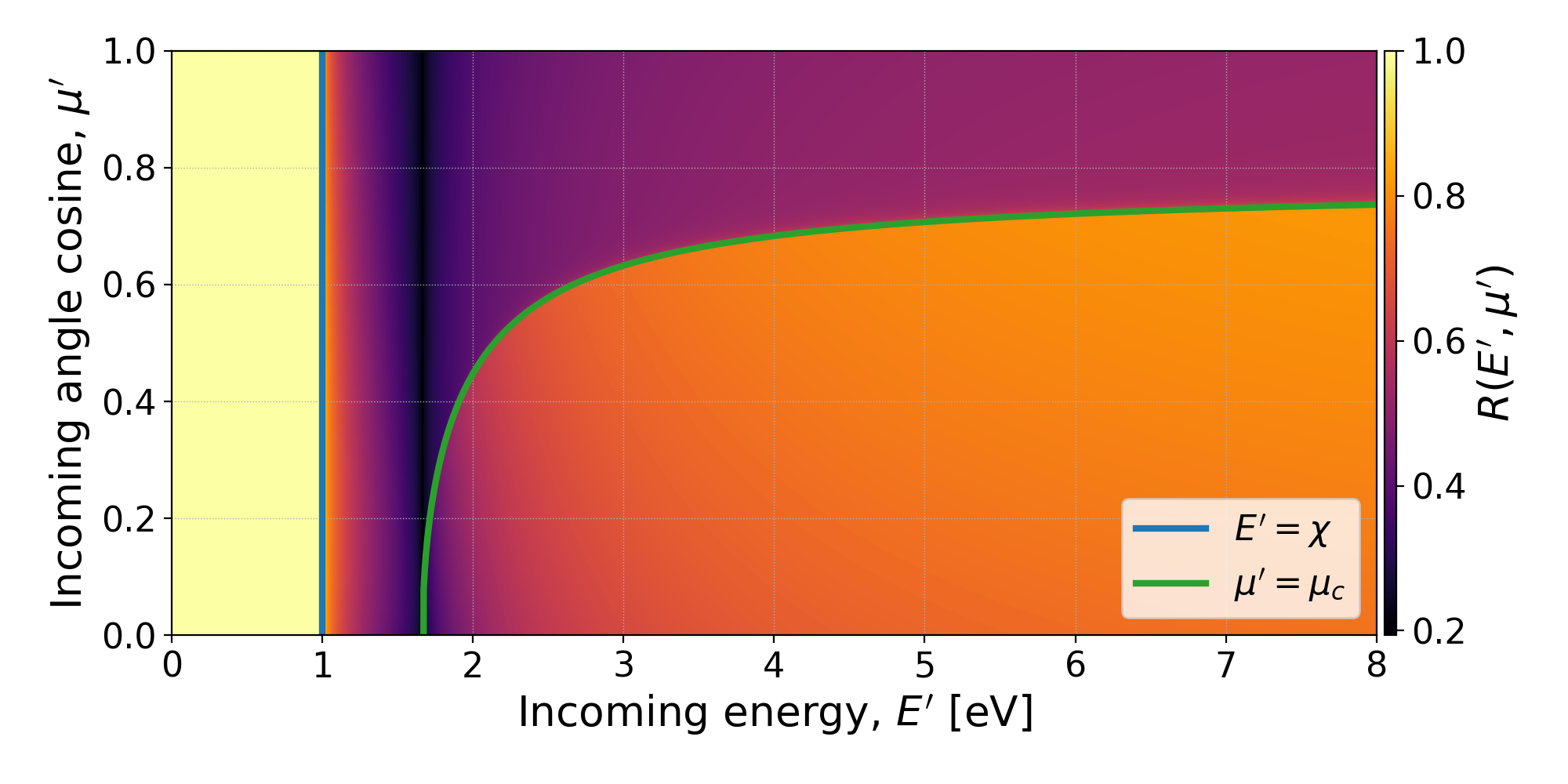
Figure 8: Probability of back-scattering, $R(E^{\prime},\mu^{\prime})$ [4] modified with the roughness coefficient $C$ (Eq. 20). Using $C=2$ and material parameters for MgO ($\chi=$1\text{\,}\mathrm{e}\mathrm{V}$$ and $\overline{m}_{\mathrm{e}}=0.4$). Figure taken from a Ph.D. dissertation [10].

The whole process can be performed as follows. The reflection function is defined as

$$R(E,\mu,E^{\prime},\mu^{\prime})=\left(1-\frac{\mathcal{T}(E^{\prime},\mu^{\prime})}{1+C/\mu^{\prime}}-\frac{C/\mu^{\prime}}{1+C/\mu^{\prime}}\int_{\mu_{c}}^{1}\mathcal{T}(E^{\prime},\mu^{\prime\prime})\,\operatorname{d\!}\mu^{\prime\prime}\right)\delta(E-E^{\prime})\delta(\mu-\mu^{\prime}).$$ (21)

Eq. (21) is converted from energetic to velocity coordinates and then substituted into the general formula in Eq. (10) and the integration over $\bm{v}^{\prime}$ is performed, which is made simple by the Dirac delta functions.

The following section (5) provides an example of implementation into the discontinuous Galerkin continuum kinetic model of the Gkeyll simulation framework.

5 Applications for Discontinuous Galerkin Simulations

The continuum kinetic boundary condition descriptions presented in this work are independent of the choice of the numerical method. Here, the discontinuous Galerkin (DG) scheme is used to develop and apply the boundary conditions described. The DG method is advantageous as it allows an arbitrarily high order representation of the solution and a small stencil size regardless of spatial order [25, 13, 16]. This section describes the implementation in the Gkeyll framework (see the A for instruction on how to get Gkeyll) and the first self-consistent continuum kinetic simulation results. DG discretization in Gkeyll is based on a novel matrix-free algorithm [publication in preparation], which makes it well suited for the implementation of phenomenological and first-principles models. The Vlasov-Maxwell solver has been used in previous work for various problems like plasma-material interactions [8, 10] and astrophysically relevant problems [9, 17, 24].

The DG scheme is developed using the principle of weak equality.

Definition 2.

Two functions, $f$ and $g$, are weakly equal if

$$\langle\psi,f-g\rangle=0,$$ (22)

where $\langle\cdot,\cdot\rangle$ is an inner product and $\psi$ is a test function. The weak equality will be denoted as $f\circeq g$.

In Gkeyll, the inner product is defined as

$$\langle\psi,f\rangle=\int_{I}f\psi\thinspace dz,$$ (23)

where $z$ corresponds to a general phase space coordinate.

The evolution equations, the Vlasov and Maxwell’s equations, need to be satisfied weakly for the DG scheme. An integration by parts is performed so the real solution can be replaced by a polynomial representation, $f_{\mathrm{h}}=\sum_{k}\hat{f}_{k}\psi_{k}$, where $\hat{f}_{k}$ are expansion coefficients corresponding to the basis function $\psi_{k}$. The Vlasov equation is then written as

$$\frac{\partial\widehat{f}_{n}^{j}(t)}{\partial t}=\left(\mathcal{M}^{j}_{nt}\right)^{-1}\Big{[}\underbracket{\widehat{f}_{m}^{j}(t)\int_{K^{j}}\bm{\alpha}_{\mathrm{h}}^{j}(\bm{z})\cdot\big{(}\psi_{m}(\bm{z})\nabla_{\bm{z}}\psi_{t}(\bm{z})\big{)}\,\operatorname{d\!}\bm{z}}_{\text{volume term}}-\underbracket{\oint_{\partial K^{j}}\bm{F}^{j}(t,\bm{z})\psi_{t}(\bm{z})\cdot\operatorname{d\!}\bm{A}}_{\text{surface term}}\Big{]},$$ (24)

where $\mathcal{M}$ is a mass matrix, $\mathcal{M}^{j}_{nt}=\int_{K^{j}}\psi_{n}\psi_{t}\,d\bm{z}$, and $\bm{\alpha}$ is a phase space vector, $\bm{\alpha}=(\bm{v},q/m(\bm{E}+\bm{v}\times\bm{B})$. Note that the integral in the volume term is only performed locally over cell $K^{j}$. The surface term is integrated over the edge of cell $K^{j}$ and includes the numerical flux function $\bm{F}$, which is a function of $f$ in the cell $K^{j}$ and $f$ in its neighbours. While the solution is allowed to be discontinuous at each cell edge, the surface term ties together an otherwise discontinuous representation.

At the domain boundaries, the surface terms could be used by prescribing the numerical flux directly at the boundaries or by including an additional layer of cells to calculate the flux in the same manner as inside the domain. These additional layers of cells are typically referred to as ghost cells. Gkeyll uses ghost cells at domain boundaries. To apply the described boundary conditions in the ghost cells, Eq. (10) becomes

$$f_{\mathrm{h}}^{g}(\bm{x}_{\text{wall}},\,\bm{v})=\sum_{s}\int_{\mathcal{V}_{\text{in}}^{s}}R^{gs}(\bm{v},\,\bm{v}^{\prime})f_{\mathrm{h}}^{s}(\bm{x}_{\text{wall}},\,\bm{v}^{\prime})\,\operatorname{d\!}\bm{v}^{\prime},$$ (25)

where the outgoing distribution function is set in the ghost layer, $f_{\mathrm{h}}^{g}$, through integration of the distribution function in the last layer of cells in the domain next to the wall, usually referred to as a skin layer, $f_{\mathrm{h}}^{s}$. Note that in the discrete case the integration is limited to one skin cell, $\mathcal{V}_{\text{in}}^{s}$, and the contributions of these integrals are added over the whole skin layer. The time dependence of the distribution functions is dropped for clarity.

Since Eq. (10) is defined only for $\bm{x}=\bm{x}^{\prime}=\bm{x}_{\text{wall}}$, the discrete representation is defined only in terms of surface basis functions $\varsigma$. Assuming, without loss of generality, that the boundary lies in the $x$-direction, incoming and outgoing distribution functions can be expressed as

$$f_{\mathrm{h}}^{g}(\bm{x},\,\bm{v})|_{x=x_{\text{wall}}}=\sum_{k}\widehat{f}_{k}^{g}\varsigma_{k}(y,z,\bm{v}),\quad f_{\mathrm{h}}^{s}(\bm{x},\,\bm{v}^{\prime})|_{x=x_{\text{wall}}}=\sum_{l}\widehat{f}_{l}^{s}\varsigma_{l}(y,z,\bm{v}^{\prime}).$$

In the discrete weak sense, Eq. (10) becomes

$$\sum_{k}\widehat{f}_{k}^{g}\varsigma_{k}(y,z,\bm{v})\circeq\sum_{s}\sum_{l}\widehat{f}_{l}^{s}\int_{\mathcal{V}_{\text{in}}^{s}}R_{\mathrm{x}}^{gs}(\bm{v},\,\bm{v}^{\prime})\varsigma_{l}(y,z,\bm{v}^{\prime})\,\operatorname{d\!}\bm{v}^{\prime}.$$

The full equality is

$$\sum_{k}\widehat{f}_{k}^{g}\int_{\partial_{x}K^{g}}\varsigma_{k}(y,z,\bm{v})\varsigma_{t}(y,z,\bm{v})\,\operatorname{d\!}y\operatorname{d\!}z\operatorname{d\!}\bm{v}=\\ =\sum_{s}\sum_{l}\widehat{f}_{l}^{s}\int_{\partial_{x}K^{s}}\int_{\mathcal{V}_{\text{in}}^{s}}R_{\mathrm{x}}^{gs}(\bm{v},\,\bm{v}^{\prime})\varsigma_{l}(y,z,\bm{v}^{\prime})\varsigma_{t}(y,z,\bm{v})\,\operatorname{d\!}\bm{v}^{\prime}\operatorname{d\!}y\operatorname{d\!}z\operatorname{d\!}\bm{v},$$ (26)

where the phase space integrals are performed over faces of the cells in the $x$-directions, $\partial_{x}K^{g,s}$. Eq. (26) is defined in the physical space and needs to be transformed into logical space for numerical implementation,

$$\sum_{k}\widehat{f}_{k}^{g}\int_{\partial_{x}I_{p}}\widehat{\varsigma}_{k}(\eta_{\mathrm{y}},\eta_{\mathrm{z}},\bm{\eta}_{\bm{v}})\widehat{\varsigma}_{t}(\eta_{\mathrm{y}},\eta_{\mathrm{z}},\bm{\eta}_{\bm{v}})\,\operatorname{d\!}\eta_{\mathrm{y}}\operatorname{d\!}\eta_{\mathrm{z}}\operatorname{d\!}\bm{\eta}_{\bm{v}}=\\ =\frac{\prod_{i=1}^{d_{v}}\Delta v_{i}}{2^{d_{v}}}\sum_{s,l}\widehat{f}_{l}^{s}\int_{\partial_{x}I_{p}}\int_{I_{v}}R_{\mathrm{x}}^{gs}\big{(}\bm{v}^{g}(\bm{\eta}_{\bm{v}}),\,\bm{v}^{s}(\bm{\eta}_{\bm{v}}^{\prime})\big{)}\widehat{\varsigma}_{l}(\eta_{\mathrm{y}},\eta_{\mathrm{z}},\bm{\eta}_{\bm{v}}^{\prime})\widehat{\varsigma}_{t}(\eta_{\mathrm{y}},\eta_{\mathrm{z}},\bm{\eta}_{\bm{v}})\,\operatorname{d\!}\bm{\eta}_{\bm{v}}^{\prime}\operatorname{d\!}\eta_{\mathrm{y}}\operatorname{d\!}\eta_{\mathrm{z}}\operatorname{d\!}\bm{\eta}_{\bm{v}},$$

where $\Delta v$ denotes the size of the cell in each dimension. For simplicity, the mesh is assumed to be uniform. For an arbitrary mesh, the Jacobian containing geometric information for each cell would be inside the summation operators. An orthonormal surface basis can be constructed, $\int_{\partial_{x}I_{p}}\tilde{\varsigma}_{k}(\eta_{\mathrm{y}},\eta_{\mathrm{z}},\bm{\eta}_{\bm{v}})\tilde{\varsigma}_{t}(\eta_{\mathrm{y}},\eta_{\mathrm{z}},\bm{\eta}_{\bm{v}})\,\operatorname{d\!}\eta_{\mathrm{y}}\operatorname{d\!}\eta_{\mathrm{z}}\operatorname{d\!}\bm{\eta}_{\bm{v}}=\delta_{kt}$. The relation simplifies to

$$\widehat{f}_{k}^{g}=\frac{\prod_{i=1}^{d_{v}}\Delta v_{i}}{2^{d_{v}}}\sum_{s,l}\widehat{f}_{l}^{s}\int_{\partial_{x}I_{p}}\int_{I_{v}}R_{\mathrm{x}}^{gs}\big{(}\bm{v}^{g}(\bm{\eta}_{\bm{v}}),\,\bm{v}^{s}(\bm{\eta}_{\bm{v}}^{\prime})\big{)}\widehat{\varsigma}_{l}(\eta_{\mathrm{y}},\eta_{\mathrm{z}},\bm{\eta}_{\bm{v}}^{\prime})\widehat{\varsigma}_{k}(\eta_{\mathrm{y}},\eta_{\mathrm{z}},\bm{\eta}_{\bm{v}})\,\operatorname{d\!}\bm{\eta}_{\bm{v}}^{\prime}\operatorname{d\!}\eta_{\mathrm{y}}\operatorname{d\!}\eta_{\mathrm{z}}\operatorname{d\!}\bm{\eta}_{\bm{v}}.$$ (27)

However, since $R^{gs}\big{(}\bm{v}^{g}(\bm{\eta}_{\bm{v}}),\,\bm{v}^{s}(\bm{\eta}_{\bm{v}}^{\prime})\big{)}$ can have a complicated dependence on $\bm{v}$ and $\bm{v}^{\prime}$, the integral on the right-hand-side of Eq. (27) cannot usually be precomputed in the logical space as can be done for volume and surface terms of the Vlasov equation. The integrals, however, do not change in time and, therefore, can be precomputed for each wall cell during the setup phase of a simulation.

Specular Reflection

As a proof of concept, the specular reflection from Eq. (11) is implemented. In the discrete case, the reflection function is limited only to cells with “opposite $x$-velocity”, symbolically denoted with Kronecker delta,

$$R_{\mathrm{x}}^{gs}(\bm{v},\bm{v}^{\prime})=\delta_{g(-s)}\delta(v_{\mathrm{x}}+v_{\mathrm{x}}^{\prime})\delta(v_{\mathrm{y}}-v_{\mathrm{y}}^{\prime})\delta(v_{\mathrm{z}}-v_{\mathrm{z}}^{\prime}).$$ (29)

Substituting this into Eq. (28) yields

$$\widehat{f}_{k}^{g}=\sum_{l}\widehat{f}_{l}^{-s}\int_{I_{p}}\widehat{\psi}_{l}(-\eta_{\mathrm{x}},\eta_{\mathrm{y}},\eta_{\mathrm{z}},-\eta_{v_{\mathrm{x}}},\eta_{v_{\mathrm{y}}},\eta_{v_{\mathrm{z}}})\widehat{\psi}_{k}(\eta_{\mathrm{x}},\eta_{\mathrm{y}},\eta_{\mathrm{z}},\eta_{v_{\mathrm{x}}},\eta_{v_{\mathrm{y}}},\eta_{v_{\mathrm{z}}})\,\operatorname{d\!}\bm{\eta}_{\bm{x}}\operatorname{d\!}\bm{\eta}_{\bm{v}}.$$ (30)

For a 1X1V (one dimension in configuration space and one dimension in velocity space) simulation with polynomial order 2, Gkeyll uses the following Serendipity [1] basis functions

$$\begin{aligned} \widehat{\psi}_{0}(\eta_{\mathrm{x}},\eta_{v_{\mathrm{x}}})&=\frac{1}{2}&\widehat{\psi}_{1}(\eta_{\mathrm{x}},\eta_{v_{\mathrm{x}}})&=\frac{\sqrt{3}\eta_{\mathrm{x}}}{2}\\ \widehat{\psi}_{2}(\eta_{\mathrm{x}},\eta_{v_{\mathrm{x}}})&=\frac{\sqrt{3}\eta_{v_{\mathrm{x}}}}{2}&\widehat{\psi}_{3}(\eta_{\mathrm{x}},\eta_{v_{\mathrm{x}}})&=\frac{3\eta_{\mathrm{x}}\eta_{v_{\mathrm{x}}}}{2}\\ \widehat{\psi}_{4}(\eta_{\mathrm{x}},\eta_{v_{\mathrm{x}}})&=\frac{\sqrt{5}(3\eta_{\mathrm{x}}^{2}-1)}{4}&\widehat{\psi}_{5}(\eta_{\mathrm{x}},\eta_{v_{\mathrm{x}}})&=\frac{\sqrt{5}(3\eta_{v_{\mathrm{x}}}^{2}-1)}{4}\\ \widehat{\psi}_{6}(\eta_{\mathrm{x}},\eta_{v_{\mathrm{x}}})&=\frac{\sqrt{15}(3\eta_{\mathrm{x}}^{2}-1)\eta_{v_{\mathrm{x}}}}{4}&\widehat{\psi}_{7}(\eta_{\mathrm{x}},\eta_{v_{\mathrm{x}}})&=\frac{\sqrt{15}\eta_{\mathrm{x}}(3\eta_{v_{\mathrm{x}}}^{2}-1)}{4}.\end{aligned}$$ (31)

Due to the orthonormality of the basis functions, the boundary condition is reduced to a simple matrix operation,

$$\mathcal{R}_{kl}=\int_{I_{p}}\widehat{\psi}_{l}(-\eta_{\mathrm{x}},-\eta_{v_{\mathrm{x}}})\widehat{\psi}_{k}(\eta_{\mathrm{x}},\eta_{v_{\mathrm{x}}})\,\operatorname{d\!}\eta_{x}\operatorname{d\!}\eta_{v_{\mathrm{x}}},$$

$$=\begin{pmatrix}1&0&0&0&0&0&0&0\\ 0&-1&0&0&0&0&0&0\\ 0&0&-1&0&0&0&0&0\\ 0&0&0&1&0&0&0&0\\ 0&0&0&0&1&0&0&0\\ 0&0&0&0&0&1&0&0\\ 0&0&0&0&0&0&-1&0\\ 0&0&0&0&0&0&0&-1\end{pmatrix}.$$

Fig. 9 presents a simple example when this boundary condition is used to let an originally Gaussian distribution of neutral particles bounce between two walls.

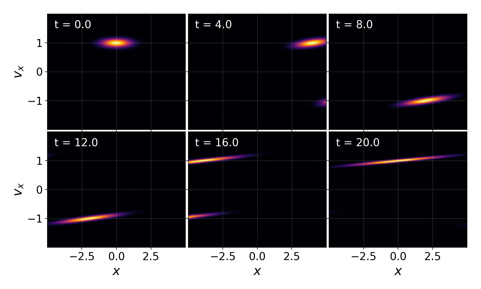
Figure 9: A test problem for the general boundary condition framework with implementation of specular reflection. An initially Gaussian distribution of neutral particles bounce between two walls in a 1D domain.

This boundary condition can be used to save computation time for symmetric problems. Plasma sheath simulations without magnetic fields where walls bound the plasma on both sides of the domain are an example of symmetric problems. Instead of simulating walls on both sides, the domain could be cut in half using a wall boundary on one side and a specular reflection to represent symmetry for the other boundary. To test this, a full domain simulation using two absorbing wall boundaries is compared with a half domain simulation which uses the specular boundary condition to capture the symmetries. The results are presented in Fig. 10. Note that the values of the distribution functions are directly subtracted and that the figure shows only the right half of the full domain simulation to allow direct calculation of the difference. Since there are regions where the distribution function is close to zero, the difference is normalized to the maximum value of the distribution. The relative difference on the order of $10^{-13}$ represents accumulated round-off error which verifies that this boundary condition implementation is correct.

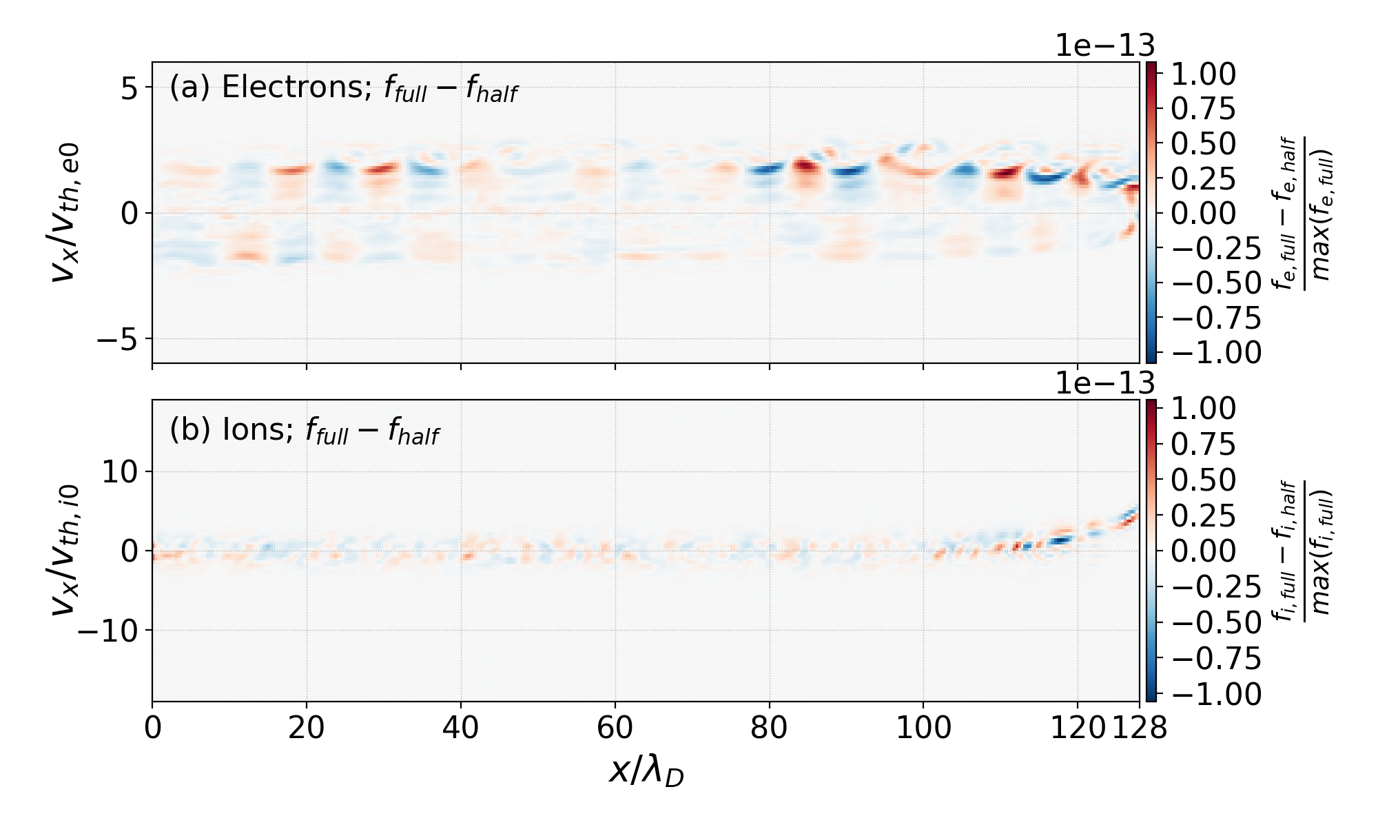
Figure 10: Normalized difference between distribution functions from the full domain (only right half is plotted) simulation using ideally absorbing walls on both sides and the half domain simulation with the specular boundary condition at the left edge replicating the symmetric behavior. Figure taken from a Ph.D. dissertation [10].

Dielectric Boundary Condition for Electrons

The boundary condition for electrons based on the model by Bronold & Fehske [4] is implemented. The integral which needs to be solved is given as

$$\mathcal{R}_{\mathrm{x},kl}^{g}=\int_{I_{p}}\left(1-\frac{\mathcal{T}\big{(}E^{g}(\bm{\eta}_{\bm{v}}),\mu^{g}(\bm{\eta}_{\bm{v}})\big{)}}{1+C/\mu^{g}(\bm{\eta}_{\bm{v}})}-\frac{C/\mu^{g}(\bm{\eta}_{\bm{v}})}{1+C/\mu^{g}(\bm{\eta}_{\bm{v}})}\int_{\mu_{\mathrm{c}}^{g}(\bm{\eta}_{\bm{v}})}^{1}\mathcal{T}(E^{g}(\bm{\eta}_{\bm{v}}),\mu^{\prime\prime})\,\operatorname{d\!}\mu^{\prime\prime}\right)\times\\ \widehat{\psi}_{l}(-\eta_{\mathrm{x}},\eta_{\mathrm{y}},\eta_{\mathrm{z}},-\eta_{v_{\mathrm{x}}},\eta_{v_{\mathrm{y}}},\eta_{v_{\mathrm{z}}})\widehat{\psi}_{k}(\eta_{\mathrm{x}},\eta_{\mathrm{y}},\eta_{\mathrm{z}},\eta_{v_{\mathrm{x}}},\eta_{v_{\mathrm{y}}},\eta_{v_{\mathrm{z}}})\,\operatorname{d\!}\eta_{\mathrm{x}}\operatorname{d\!}\eta_{\mathrm{y}}\operatorname{d\!}\eta_{\mathrm{z}}\operatorname{d\!}\eta_{v_{\mathrm{x}}}\operatorname{d\!}\eta_{v_{\mathrm{y}}}\operatorname{d\!}\eta_{v_{\mathrm{z}}}.$$ (32)

Due to the complexity of $R$ the boundary condition needs to be precomputed for each cell. As seen in Fig. 7, $R=1$ for low energies and decreases fairly rapidly as the energy increases. Therefore, it is important to be careful with constructing the velocity mesh. The electron mesh used for previous simulations [8] extends from $-6\,v_{th,e}$ to $6\,v_{th,e}$ and uses 32 cells. This puts the sharp transition at $E^{\prime}=\chi$ inside the second cell (counting from the center). As the polynomial approximation is not suited for such sharp transitions, projection of $R$ onto this mesh results in significant overshoot; see blue line in Fig. 11. However, noting the ability of the DG method to handle discontinuities and sharp gradients between the cells, the velocity mesh can be tailored for the purposes of the boundary condition. As seen by the orange line in Fig. 7, tailoring the mesh eliminates the overshoot at $v_{\mathrm{x}}\approx 0.5\,v_{th}$.

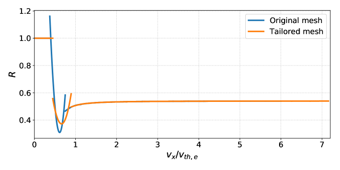
Figure 11: An example showing the projection of the reflection function given by Eq. (21) onto the simulation mesh. The same mesh is used as with previous simulations (blue line) resulting in an overshoot at $E=\chi$. The orange line shows the result when the mesh is specifically tailored for material-based boundary conditions eliminating the overshoot at $v_{\mathrm{x}}\approx 0.5\,v_{th}$. Figure taken from a Ph.D. dissertation [10].

This boundary condition can be precomputed and written as automatically generated code with expanded matrix multiplications to reduce computational cost significantly. However, because it changes based on the wall material and needs to be calculated for each cell, it is stored as an external file. As all the coefficients are precomputed and the matrix multiplication is expanded, the actual multiplication can be limited only to the non-zero terms, saving computational time substantially.

Sheath simulations are performed in 1X1V using the dielectric boundary conditions described in Sec. 4 and are compared to sheath simulations that use an ideally absorbing wall. Fig. 12 shows direct comparison (absolute difference in the electron and ion distribution functions) of the simulation with the dielectric boundary condition with the case that uses ideally absorbing walls. The solution is captured at $t\omega_{\mathrm{pe}}=500$ ($\omega_{\mathrm{pe}}$ being the electron plasma frequency) giving the simulations sufficient time to evolve from the same initial conditions. Note the periodic structure in the difference between the electron distribution functions that results due to the absence of Langmuir waves when using ideally absorbing walls. More importantly, note the higher electron density at the wall for the dielectric case due to electron emission from the wall. In the $v_{\mathrm{x}}<0$ half of the velocity domain, the acceleration of emitted electrons by the sheath electric field is visible. The ion distribution (Fig. 12b) shows that ions reach lower velocities in the sheath for a given distance from the wall with the dielectric boundary condition compared to the case with an absorbing wall.

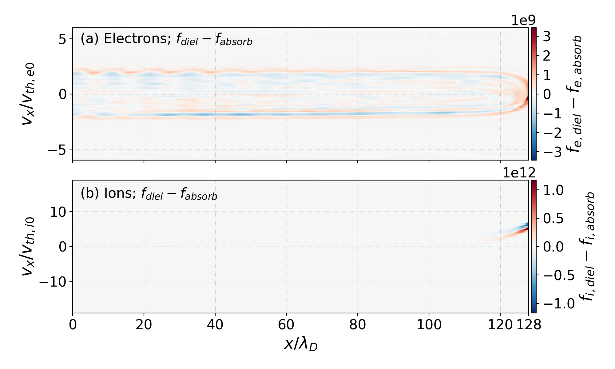
Figure 12: Direct comparison of electron and ion distribution functions from sheath simulations with absorbing and dielectric boundary conditions ($f_{diel}-f_{absorb}$). The red color denotes regions with higher particle phase space density as is the case with the dielectric wall boundary condition. The periodic structure is caused by the absence of Langmuir waves in the simulation that uses an ideally absorbing wall. Data are presented at $t\omega_{\mathrm{pe}}=500$. Figure taken from a Ph.D. dissertation [10].

Plots of electron and ion densities, ion bulk velocity, electron and ion temperatures, and electric fields are provided in Fig. 13. The simulation with the dielectric boundary condition shows roughly twice the electron density of the absorbing wall simulation in the region adjacent to the wall. Returning electrons from the dielectric wall decrease the overall outflow from the domain resulting in significantly smaller electric field needed to equalize the electron and ion fluxes as noted in Fig. 13(b). Also note that the dielectric wall reduces the potential difference between the wall and the plasma compared to the absorbing wall. The vertical solid black line in Fig. 13 marks the Bohm velocity crossing for both cases which can be considered an approximation for the sheath edge. Note that the differences between the solutions for the dielectric boundary condition and the ideally absorbing boundary condition are localized inside the sheath region. An exception is noted through the small differences in the presheath electric field caused by Langmuir waves in the absorbing wall simulations. As a result of the presheath generally being unaffected by the dielectric wall, ions have the same presheath acceleration profiles and reach the Bohm velocity at the same distance from the wall for both cases. The most significant difference is in the electron temperature (Fig. 13d) inside the sheath with lower gradients in thermal velocity for the dielectric wall compared to the absorbing wall.

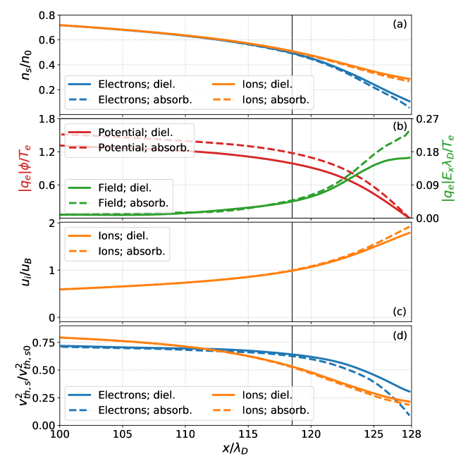
Figure 13: Comparison of profiles from sheath simulations with absorbing and dielectric wall boundary conditions. From top to bottom, panels show density (a), electric field and electrostatic potential (b), ion bulk velocity (c), and temperature (d). In each of the panels, the solid line marks simulations with the dielectric wall boundary condition based on Eq. (21) while the dashed lines corresponds to simulations with an ideally absorbing wall. Vertical dashed line marks the crossing of the Bohm velocity. Data are presented at $t\omega_{\mathrm{pe}}=500$. No collisions or ionization are included in these simulations. Figure adapted from a Ph.D. dissertation [10].

Higher moments of the distribution function are explored to understand the significant differences in the electron temperature inside the sheath between the dielectric and absorbing wall simulations. The 1X1V simulation of Fig. 13 produces a scalar value for the third moment of the distribution instead of the full heat flux tensor,

$$q_{\mathrm{e}}(x)=\frac{1}{2}m_{\mathrm{e}}\int_{-\infty}^{\infty}v_{\mathrm{x}}^{3}f_{\mathrm{e}}(x,v_{\mathrm{x}})\,\operatorname{d\!}v_{\mathrm{x}}.$$

Normalized profile of $q_{\mathrm{e}}$ in the region near the wall is shown in Fig. 14a. Due to the $v_{\mathrm{x}}^{3}$ term, the third moment is particularly sensitive to oscillations of the distribution function like the Langmuir waves discussed in previous work [10]. Therefore, the results in Fig. 14 are averaged over $\Delta t\omega_{\mathrm{pe}}=1000$.

Fig. 14a shows that the heat flux to the wall is higher for the case with the dielectric wall, which might seem to contradict the lower temperature gradients shown in Fig. 13d. However, $q_{\mathrm{e}}$ describes an energy flux, i.e., it includes the local particle density which is much higher for the case with the dielectric wall. The quantity plotted in Fig. 14a is normalized to the initial number density in the center of the domain so the result is dimensionless. Alternatively, the third moment can be normalized to the local number density, $q_{\mathrm{e}}(x)/n_{\mathrm{e}}(x)$. Fig. 14b shows this quantity compared for the dielectric and absorbing wall cases. The lower flux in the dielectric case is in agreement with the higher electron temperature and lower electron temperature gradients inside the sheath (Fig. 13d).

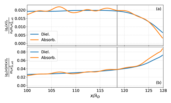
Figure 14: A comparison of heat flux profiles from the sheath simulations with absorbing and dielectric wall boundary conditions. The top panel (a) shows the third moment of the distribution function, $q_{\mathrm{e}}=\frac{1}{2}m_{\mathrm{e}}\int v_{\mathrm{x}}^{3}f_{e}\operatorname{d\!}v_{\mathrm{x}}$, normalized to initial temperature and density, while the bottom panel (b) presents $q_{\mathrm{e}}$ normalized to local density, $n_{\mathrm{e}}(x)$. The profiles are averaged over the whole course of the simulation, $\Delta t\omega_{\mathrm{pe}}=1000$.

6 Conclusions

A novel, self-consistent way to formulate boundary conditions through general reflection functions for continuum kinetic simulations is presented and its usage is demonstrated on simple specular reflection. The same framework is then used for more complex electron surface emission models—a phenomenological model [15] and a quantum mechanics based model [4].

While the formulation of the boundary condition is general, it is developed and presented using the discontinuous Galerkin method. A benchmark of a specular reflection boundary condition is implemented to reproduce central symmetry of a plasma sheath simulation with absorbing walls on both sides and no magnetic field. After letting the simulations evolve for $1000/\omega_{\mathrm{pe}}$, maximum relative differences between the full-domain case with two walls and the half-domain case with reflecting boundary conditions are on the order or $10^{-13}$, which corresponds to accumulated round-off error.

Finally, the quantum mechanics based model [4] is self-consistently implemented for simulations of classical sheaths with electron emission and is compared with an ideally absorbing wall. The results show a significant impact on electron and ion profiles as well as the electrostatic potential even for the simplest case of a one-dimensional sheath in each of the configuration and velocity space dimensions. With the novel boundary condition, electron density at the wall is doubled and electric field magnitude is roughly 40% lower in comparison to the case with ideally absorbing walls. This work presents the first description and implementation of a generalized framework to incorporate high-fidelity electron emission and surface physics boundary conditions into a continuum-kinetic plasma code.

Appendix A Getting Gkeyll and reproducing the results

To allow interested readers to reproduce our results and also use Gkeyll for their applications, this Appendix provides instructions to get the code (in both binary and source format). Full installation instructions for Gkeyll are provided on the Gkeyll website (http://gkeyll.readthedocs.io). The code can be installed on Unix-like operating systems (including Mac OS and Windows using the Windows Subsystem for Linux) either by installing the pre-built binaries using the conda package manager (https://www.anaconda.com) or building the code via sources. Input files for the simulations presented here will be made available upon request.

References

- Arnold and Awanou [2011] D.N. Arnold and G. Awanou. The Serendipity family of finite elements. Foundations of Computational Mathematics, 11(3):337–344, 2011.
- Birdsall and Langdon [2004] C.K. Birdsall and A.B. Langdon. Plasma physics via computer simulation. CRC press, 2004.
- Bohm [1949] D. Bohm. The Characteristics of Electric Discharges in Magnetic Fields. MacGraw-Hill, New York, 1949.
- Bronold and Fehske [2015] F.X. Bronold and H. Fehske. Absorption of an electron by a dielectric wall. Physical review letters, 115(22):225001, 2015.
- Bronold et al. [2018] F.X. Bronold, H. Fehske, M. Pamperin, and E. Thiessen. Electron kinetics at the plasma interface. The European Physical Journal D, 72(5):88, 2018.
- Bruining [1954] H. Bruining. Physics and Applications of Secondary Electron Emission. McGraw-Hill Book Co., 1954.
- Bruining and De Boer [1938] H Bruining and JH De Boer. Secondary electron emission: Part i. Secondary electron emission of metals. Physica, 5(1):17–30, 1938.
- Cagas et al. [2017a] P. Cagas, A. Hakim, J. Juno, and B. Srinivasan. Continuum kinetic and multi-fluid simulations of classical sheaths. Physics of Plasmas, 24(2):022118, 2017a.
- Cagas et al. [2017b] P. Cagas, A. Hakim, W. Scales, and B. Srinivasan. Nonlinear saturation of the Weibel instability. Physics of Plasmas, 24(11):112116, 2017b.
- Cagas [2018] Petr Cagas. Continuum Kinetic Simulations of Plasma Sheaths and Instabilities. PhD thesis, Virginia Tech, 2018.
- Campanell and Umansky [2016] M.D. Campanell and M.V. Umansky. Strongly emitting surfaces unable to float below plasma potential. Physical review letters, 116(8):085003, 2016.
- Campanell et al. [2012] M.D. Campanell, A.V. Khrabrov, and I.D. Kaganovich. General cause of sheath instability identified for low collisionality plasmas in devices with secondary electron emission. Phys. rev. let., 108(23):235001, 2012. doi: 10.1103/PhysRevLett.108.235001.
- Cockburn and Shu [2001] B. Cockburn and C.-W. Shu. Runge-Kutta discontinuous Galerkin methods for convection-dominated problems. Journal of scientific computing, 16(3):173–261, 2001.
- Dunaevsky et al. [2003] A. Dunaevsky, Y. Raitses, and N.J. Fisch. Secondary electron emission from dielectric materials of a Hall thruster with segmented electrodes. Physics of Plasmas, 10(6):2574–2577, 2003. doi: 10.1063/1.1568344.
- Furman and Pivi [2002] M.A. Furman and M.T.F. Pivi. Probabilistic model for the simulation of secondary electron emission. Physical Review Special Topics-Accelerators and Beams, 5(12):124404, 2002.
- Hesthaven and Warburton [2004] J.S. Hesthaven and T. Warburton. High-order nodal discontinuous Galerkin methods for the Maxwell eigenvalue problem. Philosophical Transactions of the Royal Society of London A: Mathematical, Physical and Engineering Sciences, 362(1816):493–524, 2004.
- Juno and Hakim [2018] J. Juno and A. Hakim. Generating a quadrature and matrix-free discontinuous Galerkin algorithm for (plasma) kinetic equations. in preparation, 2018.
- Kaganovich et al. [2007] I.D. Kaganovich, Y. Raitses, D. Sydorenko, and A. Smolyakov. Kinetic effects in a Hall thruster discharge. Physics of Plasmas, 14(5):057104, 2007. doi: 10.1063/1.2709865.
- Langmuir [1923] I. Langmuir. The effect of space charge and initial velocities on the potential distribution and thermionic current between parallel plane electrodes. Phys. Rev., 21:954, 1923. doi: 10.1103/PhysRev.21.419.
- Loizu et al. [2012] J. Loizu, P. Ricci, F.D Halpern, and S. Jolliet. Boundary conditions for plasma fluid models at the magnetic presheath entrance. Physics of Plasmas, 19(12):122307, 2012.
- Mikellides et al. [2013] Ioannis G Mikellides, Ira Katz, Richard R Hofer, and Dan M Goebel. Magnetic shielding of walls from the unmagnetized ion beam in a Hall thruster. Applied Physics Letters, 102(2):023509, 2013.
- Mutsukura et al. [1990] Nobuki Mutsukura, Kenji Kobayashi, and Yoshio Machi. Plasma sheath thickness in radio-frequency discharges. Journal of Applied Physics, 68(6):2657–2660, 1990.
- Nicholson [1983] D.R. Nicholson. Introduction to plasma theory. John Wiley and Sons, Inc., 1983. ISBN 0-471-09045-X.
- Pusztai et al. [2018] Istvan Pusztai, Jason M TenBarge, Aletta N Csapó, James Juno, Ammar Hakim, Longqing Yi, and Tünde Fülöp. Low Mach-number collisionless electrostatic shocks and associated ion acceleration. Plasma Physics and Controlled Fusion, 60(3):035004, 2018.
- Reed and Hill [1973] W.H. Reed and T.R. Hill. Triangular mesh methods for the neutron transport equation. Technical report, Los Alamos Scientific Lab., N. Mex.(USA), 1973.
- Riemann [1991] K.-U. Riemann. The Bohm criterion and sheath formation. J. Phys. D: Appl. Phys., 24:493–518, 1991. doi: 10.1088/0022-3727/24/4/001.
- Robertson [2013] S. Robertson. Sheaths in laboratory and space plasmas. Plasma Phys. Control. Fusion, 55:93001, 2013. doi: 10.1088/0741-3335/55/9/093001.
- Rosenbluth et al. [1957] Marshall N Rosenbluth, William M MacDonald, and David L Judd. Fokker-planck equation for an inverse-square force. Physical Review, 107(1):1, 1957.
- Schwager [1993] LA Schwager. Effects of secondary and thermionic electron emission on the collector and source sheaths of a finite ion temperature plasma using kinetic theory and numerical simulation. Physics of Fluids B: Plasma Physics, 5(2):631–645, 1993.
- Sheehan et al. [2013] JP Sheehan, N Hershkowitz, ID Kaganovich, He Wang, Y Raitses, EV Barnat, BR Weatherford, and D Sydorenko. Kinetic theory of plasma sheaths surrounding electron-emitting surfaces. Physical review letters, 111(7):075002, 2013.
- Smith et al. [1998] D.L. Smith, E.Y. Lee, and V. Narayanamurti. Ballistic electron emission microscopy for nonepitaxial metal/semiconductor interfaces. Physical review letters, 80(11):2433, 1998.
- Stangeby [2000] P.C. Stangeby. The Plasma Boundary of Magnetic Fusion Devices. Institute of Physics Publishing, Bristol and Philadelphia, 2000. ISBN 0 7503 0559 2.
- Sydorenko et al. [2006] D. Sydorenko, A. Smolyakov, I. Kaganovich, and Y. Raitses. Kinetic simulation of secondary electron emission effects in Hall thrusters. Phys. of Plas., 13(1):014501, 2006. doi: 10.1063/.2158698.
- Takamura et al. [2004] S. Takamura, N. Ohno, M.Y. Ye, and T. Kuwabara. Space-charge limited current from plasma-facing material surface. Contributions to Plasma Physics, 44(1-3):126–137, 2004. doi: 10.1002/ctpp.200410017.
- Tang and Guo [2017] Xian-Zhu Tang and Zehua Guo. Bohm criterion and plasma particle/power exhaust to and recycling at the wall. Nuclear Materials and Energy, 12:1342–1347, 2017.
- Tang [2011] X.Z. Tang. Kinetic magnetic dynamo in a sheath-limited high-temperature and low-density plasma. Plasma Physics and Controlled Fusion, 53(8):082002, 2011.