Friedel oscillations of one-dimensional correlated fermions from perturbation theory and density functional theory

Abstract

We study the asymptotic decay of the Friedel density oscillations induced by an open boundary in a one-dimensional chain of lattice fermions with a short-range two-particle interaction. From Tomonaga-Luttinger liquid theory it is known that the decay follows a power law, with an interaction dependent exponent, which, for repulsive interactions, is larger than the noninteracting value $-1$. We first investigate if this behavior can be captured by many-body perturbation theory for either the Green function or the self-energy in lowest order in the two-particle interaction. The analytic results of the former show a logarithmic divergence indicative of the power law. One might hope that the resummation of higher order terms inherent to the Dyson equation then leads to a power law in the perturbation theory for the self-energy. However, the numerical results do not support this. Next we use density functional theory within the local-density approximation and an exchange-correlation functional derived from the exact Bethe ansatz solution of the translational invariant model. While the numerical results are consistent with power-law scaling if systems of $10^{4}$ or more lattice sites are considered, the extracted exponent is very close to the noninteracting value even for sizeable interactions.

1 Introduction

The elementary excitations of one-dimensional (1d), metallic Fermi systems with a two-particle interaction are not given by fermionic quasi-particles, but are instead of collective, bosonic nature Schoenhammer05 ; Giamarchi03 . Such quantum many-body systems can thus not be described by Fermi liquid theory. For short-ranged, i.e. screended, two-particle interactions, on which we focus here, Tomonaga-Luttinger liquid theory is applicable instead Haldane81 . One of the characteristics of Tomonaga-Luttinger liquids is the power-law decay of correlation functions at large times or spatial distances with exponents which, in spinless models, can be expressed in terms of a single parameter $K$. This Tomonaga-Luttinger liquid parameter depends on the band structure and filling as well as on the amplitude and range of the two-particle interaction of the model Hamiltonian. For repulsive interactions $0<K<1$ while $K>1$ for attractive ones; $K=1$ corresponds to noninteracting fermions.

To exemplify the Tomonaga-Luttinger liquid behavior let us focus on the observable of interest to us, which is the density $n(x)$. Depending on the model considered the spatial variable $x$ might be continuous or given by a lattice site index $x\to j=1,2,\ldots,L$ and $L$ being the system size (the lattice spacing is set to 1). We consider a system with open boundary conditions in which translational invariance is broken. Generically, $n(x)$ shows oscillations which decay from the boundaries towards the middle, the bulk part of the chain, at which the average density $\nu$ is reached. From Tomonaga-Luttinger liquid theory it is known that $n(x)-\nu$ decays as $x^{-K}$ and oscillates with (spatial) frequency $2k_{\rm F}$, with the Fermi momentum $k_{\rm F}$ ($\hbar=1$) Fabrizio95 ; Egger95 . For a single-band lattice model $k_{\rm F}=\nu\pi$. These are the famous Friedel oscillations with an exponent which, however, is modified by the interaction as compared to the noninteracting value $-1$ ($-d$ in $d$ dimensions). For repulsive interactions the oscillations decay slower while they decay faster for attractive ones.

For the lattice model of spinless fermions with nearest-neighbor hopping $t$ and nearest-neighbor density-density interaction $U$ considered here, in the thermodynamic limit $K(\nu,U/t)$ can be expressed in terms of a set of coupled integral equations derived from the Bethe ansatz solution of this model Haldane80 . At half-filling, $\nu=1/2$, a closed-form expression for $K(\nu,U/t)$ can be derived. For $-2<U/t<2$ the model is in a metallic Tomonaga-Luttinger liquid phase while for $|U|/t>2$ insulating phases are found. Away from half-filling the model is a Tomonaga-Luttinger liquid for all $U/t>-2$. However, the integral equations can only be solved numerically (with high precision) and accordingly $K(\nu,U/t)$ is only known numerically. We will refer to this as the exact Tomonaga-Luttinger liquid parameter.

It is generally believed that approximate approaches to the quantum many-body problem which lead to an effective fermionic single-particle picture, such as, e.g., lowest order perturbation theory, will generically fail to capture Tomonaga-Luttinger liquid behavior of correlation functions. Such approaches appear to be at odds with the absence of fermionic quasi-particles in Tomonaga-Luttinger liquids. An exception to this is the local single-particle spectral function as a function of frequency on lattice sites close to an open boundary. For this the lowest order perturbation theory in $U$ for the self-energy, i.e. the non-self-consistent Hartree-Fock approximation, leads to a power-law suppression in accordance with Tomonaga-Luttinger liquid theory Meden00 . Motivated by this we investigate if the same holds for the decay of the density oscillations away from an open boundary and into the bulk of the chain. Lowest order perturbation theory for the Green function shows a logarithmic position dependence consistent with the power law. However, the numerical non-self-consistent Hartree-Fock data do not support that the resummation of higher-order terms inherent to the Dyson equation does elevate this logarithmic term to a power law.

Next, we study if the power-law decay of the density with an interaction dependent exponent can be obtained within (lattice Gunnarsson86 ; Schoenhammer95 ; Lima03 ; Schmitteckert_Evers_2008 ) density functional theory (DFT) Hohenberg64 , an approach which also builds on an effective single-particle picture. We employ the local density approximation extracted from the ground-state energy obtained from the Bethe ansatz (BALDA) solution of the lattice model. For a different lattice model this approach was first suggested in Ref. Schoenhammer95 .

In Ref. Schenk08 BALDA-DFT was used to investigate the static and dynamic response of the translational invariant (periodic boundary conditions) lattice model described above as well as the behavior of this model if a single impurity is introduced. The authors concluded that Tomonaga-Luttinger liquid behavior is not captured. However, they did not search for the characteristic power-law scaling of correlation functions and were bound to systems of only a few hundred lattice sites (see below).

The two observables which are most directly accessible within a DFT approach are the ground-state energy and the ground-state density. Here, we study the latter for systems of up to $10^{6}$ lattice sites; the former does not contain any Tomonaga-Luttinger liquid power laws Schoenhammer05 ; Giamarchi03 . The characteristic Tomonaga-Luttinger liquid behavior induced by an open boundary is much less involved than the one resulting from a localized impurity (renormalization group flow of the impurity towards an open boundary) Luther74 ; Apel82 ; Kane92 ; Egger95 . Posing the question if BALDA-DFT can correctly describe the decay of the Friedel oscillations due to an open boundary, as we do here, thus constitutes less of a challenge to this method as compared to the problems investigated in Ref. Schenk08 . With a different emphasize to ours the perspectives of using Hartree-Fock and DFT to study Friedel oscillations in 1d correlated fermions were also investigated in Ref. Sch

With the hard wall boundary replaced by a local impurity Friedel oscillations were investigated for the 1d (spinful) Hubbard model in Ref. Lima03 employing BALDA-DFT. The density for lattices of a few hundred lattice sites was computed. For the local single-particle spectral function it is well established that to unambiguously observe asymptotic Tomonaga-Luttinger liquid power-law behavior much larger system sizes (of the order of $10^{4}$ to $10^{5}$ sites) are required even in the most simple case of spinless fermions with open boundaries; see e.g. Ref. Andergassen04 . The same is expected to hold for the decay of the density oscillations; see below for explicit results on this. For smaller systems the asymptotics is completely masked by finite size effects. The study of Ref. Lima03 faces two additional challenges: (1) Due to the logarithmically slow vanishing of the two-particle backscattering of particles with opposite spin for increasing system size Solyom79 , even larger systems than for spinless models are required to observe power laws in the Hubbard model, see e.g. Refs. Andergassen06 ; Soeffing13 . (2) The finite local impurity of Ref. Lima03 requires larger systems to observe the asymptotic density decay than the open boundary, see e.g. Refs. Kane92 ; Egger95 ; Andergassen04 ; Andergassen06 . It was thus premature to fit the density decay obtained in Ref. Lima03 by a power law. Not surprisingly, the exponents obtained for repulsive interactions are smaller than $-1$ and, therefore, contradict Tomonaga-Luttinger liquid theory.

Our numerical BALDA-DFT data for the density decay away from the open boundary for the above lattice model of spinless fermions turn out to be consistent with power-law scaling if system sizes of $10^{4}$ or more lattice sites are considered. However, the exponent extracted is very different from the exact Tomonaga-Luttinger liquid parameter. Even for sizeable interactions the data appear to be consistent with the noninteracting value $-1$.

The remainder of this paper is organized as follows. In Sect. 2 we present our model and give basics on the methods used to compute the density. Our results obtained by the three approaches, i.e. lowest order perturbation theory for the Green function, the non-self-consistent Hartree-Fock approximation as well as the BALDA-DFT, are presented in the three subsections of Sect. 3. Details on the analytical calculations for the Green function perturbation theory are given in the Appendix. We conclude in Sect. 4.

2 The model and methods

2.1 Spinless lattice fermions

We study the 1d model of spinless fermions with nearest-neighbor hopping $t>0$ and nearest-neighbor interaction $U$ between particles occupying the Wannier states with lattice site index $j$. It is given by the Hamiltonian

$$H=-t\sum_{j=1}^{L-1}\left(c_{j+1}^{\dagger}c_{j}^{\phantom{{\dagger}}}+\mbox{H.c.}\right)+U\sum_{j=1}^{L-1}n_{j}n_{j+1}$$ (1)

in standard second quantized notation, where $n_{j}=c_{j}^{\dagger}c_{j}^{\phantom{{\dagger}}}$ is the density operator on site $j$ and $L$ denotes the number of lattice sites. Note the open boundary conditions.

In the noninteracting case, $U=0$, the single-particle eigenfunctions $\left|n\right>$, with $n\in\{1,2,...,L\}$ are given by

$$\langle j|n\rangle=\sqrt{\frac{2}{L+1}}\sin{(k_{n}j)},\quad k_{n}=\frac{n\pi}{(L+1)}.$$ (2)

The single-particle energies are $\epsilon(k)=-2t\cos{k}$. The many-body ground state for band filling $\nu=N/L$ is given by the Slater determinant build out of the first $N$ single-particle states.

The ground-state expectation value of the density can, for arbitrary $U$, be computed from the (zero temperature) Matsubara Green function $G_{j,j^{\prime}}(\omega)$ as

$$n(j)=\langle n_{j}\rangle=\frac{1}{2}+\frac{1}{\pi}\int\limits_{0}^{\infty}d\omega\,{\rm Re}\,G_{j,j}(i\omega).$$ (3)

For $U=0$ the Green function in the single-particle eigenbasis $\left\{\left|n\right>\right\}$ is given by

$$G^{0}_{n,n^{\prime}}=[i\omega-\xi(k_{n})]^{-1}\delta_{n,n^{\prime}},$$ (4)

where $\xi(k)=\epsilon(k)-\mu$, with the chemical potential $\mu$. Changing to this basis and inserting $G^{0}$, the integral in Eq. (3) can be performed leading to ($j=1,2,\ldots,L$)

$$n^{0}(j)=\frac{2N+1}{2(L+1)}-\frac{1}{2(L+1)}\frac{\sin{\left(\frac{\pi}{L+1}j\left[2N+1\right]\right)}}{\sin{\left(\frac{\pi}{L+1}j\right)}}.$$ (5)

In the thermodynamic limit $L,N\rightarrow\infty$, $\nu=N/L$ fixed, the noninteracting density reduces to

$$n^{0}(j)=\nu-\frac{\sin{(2k_{{\rm F}}j)}}{2\pi j}.$$ (6)

These are the well known Friedel oscillations with wave vector $2k_{\rm F}$ which, in a noninteracting 1d system, decay as $1/j$.

Note that for half filling, $\nu=1/2$, of the lattice the oscillatory part of the density vanishes in both the finite system result Eq. (5) as well as in the $L\to\infty$ result Eq. (6) and $n^{0}(j)=1/2$. The same holds for $U\neq 0$ Kitanine08 .

2.2 The Bethe ansatz solution and Tomonaga-Luttinger liquid properties

For $U\neq 0$ the model Eq. (1) with periodic boundary conditions is Bethe ansatz solvable (see e.g. Ref. Giamarchi03 ). In the thermodynamic limit this allows one to formulate a closed set of integral equations from which the ground-state energy and other quantities of interest can be obtained. The results derived along this line are consistent with the assumption that the model falls into the Tomonaga-Luttinger liquid universality class for $\nu\neq 1/2$ and all $U/t>-2$ as well as for $-2<U/t<2$ at half filling $\nu=1/2$ Haldane80 . We focus on this Tomonaga-Luttinger liquid regime.

The solvability by Bethe ansatz does, however, not imply that explicit analytic expressions for correlation functions showing the characteristic Tomonaga-Luttinger liquid power laws can be derived. Computing correlation functions by numerical methods (for particularly convincing results, see Ref. Karrasch12 ) as well as renormalization group approaches (see e.g. Refs. Giamarchi03 ; Solyom79 ; Andergassen04 ; Schmitteckert_Eckern_1996 ) it was still unambiguously confirmed that, for the above parameter regime, the model is a Tomonaga-Luttinger liquid. The corresponding asymptotic decay of the Friedel oscillations off an open boundary

$$\left|n^{\rm TL}(j)-\nu\right|\sim\frac{\sin{(2k_{{\rm F}}j)}}{j^{K}},$$ (7)

as described in Sect. 1, was explicitely confirmed for the present model in Ref. Andergassen04 .

For $\nu\neq 1/2$ results for the Tomonaga-Luttinger liquid parameter $K(\nu,U/t)$ can be obtained from numerically solving the Bethe ansatz integral equations Haldane80 . To leading order in $U/t$ one finds Meden00 ; Giamarchi03

$$K=1-\frac{U}{\pi v_{\rm F}}\left[1-\cos\left(2k_{\rm F}\right)\right]+{\mathcal{O}}\left([U/t]^{2}\right),$$ (8)

with the Fermi velocity $v_{\rm F}=2t\sin k_{\rm F}$. For $\nu=1/2$ a closed analytical expression for $K(1/2,U/t)$ can be derived even beyond the leading order. However, as already indicated by the absence of Friedel oscillations for $U=0$ [see Eqs. (5) and (6)], half-filling is nongeneric if it comes to density oscillations and thus of minor interest to us.

2.3 The Bethe ansatz solution and LDA-DFT

The Bethe ansatz integral equations for the translational invariant model can also be used within a Bethe ansatz (BA)LDA-DFT approach to derive an exchange-correlation functional.

In a practical implementation of the DFT idea one constructs an auxiliary, noninteracting Kohn-Sham Hamiltonian Sham66

$$H^{\rm KS}=-t\sum_{j=1}^{L-1}\left(c_{j+1}^{\dagger}c_{j}^{\phantom{{\dagger}}}+\mbox{H.c.}\right)+\sum_{j=1}^{L-1}v_{j}n_{j},$$ (9)

with the onsite potential $v_{j}$ chosen such that it leads to the same density $n(j)$ as in the interacting problem. The single-particle potential is written as $v_{j}=v_{j}^{\rm H}+v_{j}^{\rm xc}$ with the Hartree potential $v_{j}^{\rm H}=U\left[n(j+1)+n(j-1)\right]$ and the exchange-correlation potential on site $j$

$$v_{j}^{{\rm xc}}=\frac{\partial}{\partial n}\Big{[}e^{{\rm BA}}(n,U)-e^{{\rm H}}(n,U)\Big{]}_{n=n(j)}$$ (10)

where $e^{{\rm BA}}(n,U)$ is the Bethe ansatz ground-state energy per site of the homogeneous system with density $n$ and interaction strength $U$. The other term is the Hartree energy given by $e^{{\rm H}}(n,U)=-\frac{2t}{\pi}\sin{(k_{{\rm F}})}+Un^{2}$. The exchange-correlation potential is computed numerically solving the Bethe ansatz integral equations. The derivative in Eq. (10) is approximated by centered differences. For a plot of $v^{{\rm xc}}$ as a function of the density at different $U/t$ for our model, see Fig. 1 of Ref. Schenk08 .

When numerically solving the DFT self-consistency problem, instead of following the standard procedure of diagonalizing the single-particle Kohn-Sham Hamiltonian Eq. (9) and subsequently computing the density from the Kohn-Sham single-particle eigenstates, we here proceed differently. To compute the $(j,j)$ matrix element of the Green function of the Kohn-Sham system, from which $n^{\rm DFT}(j)$ can be obtained by Eq. (3), we only have to determine the diagonal part of the inverse of the tri-diagonal matrix associated to $H^{\rm KS}$. As described in Appendix C of Ref. Andergassen04 this can be achieved in ${\mathcal{O}}(L)$ time ($L$ is the system size and thus the size of the resolvent matrix) and is thus much faster and requires less memory as compared to a diagonalization. We note that we implement the integration of Eq. (3) as the solution of a differential equation (for more details see Odavic19 ). All this allows us to study systems of up to $10^{6}$ lattice sites (at sizeable filling) not accessible following the standard procedure. In particular, we are able to study much larger systems as compared to the ones investigated in Refs. Schenk08 (spinless fermions) and Lima03 (Hubbard model). We believe that this approach might also be useful in other DFT applications. The self-consistency cycle of DFT was stopped when the change of the density summed over all lattice sites was less than $10^{-5}$. The convergence is achieved in about 10 to 20 cycles, when performing the usual linear mixing of the density.

Results for the density profile obtained along these lines are presented in Sect. 3.3.

2.4 Perturbation theory

Many-body perturbation theory in lowest order in $U/t$ provides an alternative way to obtain approximate results for the density. We compute the self-energy $\Sigma$ to first order in $U/t$ (non-self-consistent Hartree-Fock approximation). To this order it becomes (Matsubara-) frequency independent. Within the Wannier basis $\Sigma^{\rm 1PT}$ is a tri-diagonal matrix with the diagonal (Hartree term) given by

$$\Sigma_{j,j}^{\rm 1PT}\!=\!-U\!\!\times\!\!\left\{\begin{array}[]{ll}\!\!n^{0}(2)&\!\mbox{for}\,j=1\\ \!\!\left[n^{0}(j-1)+n^{0}(j+1)\right]&\!\mbox{for}\,j=2,\ldots,L-1\\ \!\!n^{0}(L-1)&\!\mbox{for}\,j=L,\end{array}\right.$$ (11)

with $n^{0}(j)$ stated in Eq. (5). The upper first off-diagonal (Fock term) reads

$$\Sigma_{j,j+1}^{\rm 1PT}= \frac{U}{2(L+1)}\left\{\frac{\sin{\left[\frac{\pi}{L+1}\left(N+\frac{1}{2}\right)\right]}}{\sin\left[\frac{\pi}{2(L+1)}\right]}\right.$$

$$-\left.\frac{\sin{\left[\frac{\pi}{L+1}\left(N+\frac{1}{2}\right)\left(2j+1\right)\right]}}{\sin\left[\frac{\pi}{2(L+1)}(2j+1)\right]}\right\},$$ (12)

with $j=1,2,\ldots,L-1$. The lower first off-diagonal follows from $\Sigma^{\dagger}=\Sigma$. To obtain the non-self-consistent Hartree-Fock approximation for the Green function

$$G^{\rm HF}=\left[\left(G^{0}\right)^{-1}-\Sigma^{\rm 1PT}\right]^{-1}$$ (13)

and from this $n^{\rm HF}(j)$ employing Eq. (3), we thus have to solve a noninteracting single-particle problem with an effective bond-dependent nearest-neighbor hopping $t-\Sigma^{\rm 1PT}_{j,j+1}$ and the effective site-dependent onsite energy $\Sigma^{\rm 1PT}_{j,j}$. Due to the involved $j$ dependence of the hopping and onsite energy, reflecting the Friedel oscillations of the noninteracting density $n^{0}(j)$, this cannot be achieved analytically. As in BALDA-DFT we refrain from numerically diagonalizing the effective single-particle Hamiltonian and instead exploit that to compute $n^{\rm HF}(j)$ we only need the diagonal part of the inverse of a tri-diagonal matrix which can be determined numerically in ${\mathcal{O}}(L)$ Andergassen04 . For results, see Sect. 3.2.

To gain analytical insights we expand Eq. (13) to first order in $U$ (first order perturbation theory for the Green function)

$$G^{\rm 1PT}=G^{0}+G^{0}\Sigma^{\rm 1PT}G^{0}$$ (14)

which, using Eq. (3), leads to a first order approximation for the density $n^{\rm 1PT}(j)$. For analytical calculations it is advantageous to work in the basis of the single-particle eigenfunctions $\left\{\left|n\right>\right\}$ of the noninteracting Hamiltonian Eq. (2) in which $G^{0}$ is diagonal; see Eq. (4). We thus have to compute $\Sigma^{\rm 1PT}$ in this basis instead of the Wannier basis as done in Eqs. (11) and (2.4). Details on this and the corresponding results for $n^{\rm 1PT}(j)$ are discussed in Sect. 3.1 and the Appendix (see also Ref. Meden00 ).

3 Results for the density decay

We next present our results for the density decay employing the three approximate approaches discussed in the last section. As mentioned in the Introduction it is commonly believed that Tomonaga-Luttinger liquid power laws, e.g. the one of Eq. (7) found for the decay of the Friedel oscillations, cannot be obtained by approaches based on effective fermionic single-particle pictures. We will show that the analytical results of the first order perturbation theory for the Green function $n^{\rm 1PT}(j)$ indicate the TLL power law by showing a logarithmic $j$ dependence. More cannot be expected within this approximation. The numerical results for the non-self-consistent Hartree-Fock approximation $n^{\rm HF}(j)$ do not support that the logarithmic behavior is elevated to a power law by the resummation inherent to the use of the Dyson equation (13). The numerical BALDA-DFT results for the density $n^{\rm DFT}(j)$ are consistent with power-law scaling, however, with an exponent which is very close to the noninteracting value $-1$ even for sizeable two-particle interactions.

3.1 Perturbation theory for the Green function

To see what to expect when computing $n^{\rm 1PT}(j)$ we first expand the Tomonaga-Luttinger liquid result Eq. (7) using the leading order expression for the Tomonaga-Luttinger liquid parameter $K$ Eq. (8). For $k_{\rm F}\neq\pi/2$, i.e. $\nu\neq 1/2$, this leads to

$$\!\!\!\!\!\!\left|n^{\rm TL}(j)-\nu\right| \sim\frac{\sin{(2k_{{\rm F}}j)}}{j}\left\{1+\frac{U}{\pi v_{\rm F}}\left[1-\cos\left(2k_{\rm F}\right)\right]\ln j\right\}$$

$$+{\mathcal{O}}(\left(\left[U/t\right]^{2}\right).$$ (15)

The appearance of a $\ln j$ term in $n^{\rm 1PT}(j)$, with a prefactor which corresponds to the negative of the leading order correction of $K$ Eq. (8), would thus provide an indication of Tomonaga-Luttinger liquid behavior. In lowest order perturbation theory for the Green function we strictly expand the density to first order in $U/t$ and thus cannot expect more, such as, e.g., a power law with a $U$ dependent exponent. The case of half-filling is excluded as the prefactor in front of the curly brackets on the right hand side of Eq. (3.1) would vanish. As already mentioned in Sect. 2.1 for a half-filled band nongeneric behavior of the density is found Kitanine08 and from now on we exclude this from our considerations. Results for $\nu=1/2$ are presented in Ref. Odavic19 .

Following Ref. Meden00 the self-energy in the basis of the single-particle eigenfunctions can be written as

$$\frac{(L+1)\Sigma^{{\rm 1PT}}_{n,n^{\prime}}}{U} =\!\Bigg{\{}2N-\sum\limits_{m=1}^{N}\Big{[}\cos{(k_{n}-k_{m})}+\cos{(k_{n}+k_{m})}\Big{]}\!\Bigg{\}}\delta_{n,n^{\prime}}-\Bigg{\{}\cos{(k_{n}-k_{n^{\prime}})}-\cos{\Bigg{(}\frac{k_{n}+k_{n^{\prime}}}{2}\Bigg{)}}\Bigg{\}}f\Bigg{(}\frac{|n-n^{\prime}|}{2}\Bigg{)}$$

$$+\Bigg{\{}\cos{(k_{n}+k_{n^{\prime}})}-\cos{\Bigg{(}\frac{k_{n}-k_{n^{\prime}}}{2}\Bigg{)}}\Bigg{\}}f\Bigg{(}\frac{n+n^{\prime}}{2}\Bigg{)}$$ (16)

with

$$f(x)\!=\!\!\left\{\begin{array}[]{ll}\!1&\quad\!\!{\rm for}\quad x\leq N\,\wedge\,x\in\mathbb{N}\\ \!0&\quad\!\!{\rm otherwise}\end{array}\right.$$ (17)

We here already neglected terms with an additional prefactor $1/L$ which are irrelevant as we later take the thermodynamic limit. Note that contributions from umklapp scattering, only present for $\nu=1/2$, are suppressed.

To illustrate the effect of the two-particle interaction we first consider the diagonal part $\Sigma^{{\rm 1PT}}_{n,n}$. For $L\to\infty$ it is given by

$$\Sigma^{{\rm 1PT}}_{k,k}=2U\nu-\frac{2U}{\pi}\sin{(\pi\nu)}\cos{k}.$$ (18)

The first addend is a $U$ dependent shift of the chemical potential. The second one can be combined with the noninteracting single-particle dispersion $\epsilon(k)=-2t\cos{k}$ to a $U$ dependent change of the hopping $\bar{t}=t+\frac{U}{\pi}\sin(\pi\nu)$. In a translational invariant setup (periodic boundary conditions) all other matrix elements of the self-energy vanish and on non-self-consistent Hartree-Fock level the effect of the interaction reduces to a shift of the chemical potential and a change of the band width from $4t$ to $4\bar{t}$ (broadening of the band for repulsive interactions $U>0$).

To obtain $n^{\rm 1PT}(j)$ we separate the noninteracting density $n^{0}(j)$ and the first order correction $\Delta n^{\rm 1PT}(j)\propto U/t$ such that $n^{\rm 1PT}(j)=n^{0}(j)+\Delta n^{\rm 1PT}(j)$. Employing Eqs. (14) as well as (3) and performing the integral over $\omega$ we obtain for $L\to\infty$

$$\Delta n^{{\rm 1PT}}(j)=\frac{U}{t\pi^{2}}\int_{0}^{k_{{\rm F}}}dk\int_{k_{{\rm F}}}^{\pi}dk^{\prime}\frac{\sin{(kj)}\sin{(k^{\prime}j)}}{\cos{(k^{\prime})}-\cos{(k)}}\sigma^{{\rm 1PT}}_{k,k^{\prime}},$$ (19)

with

$$\sigma^{{\rm 1PT}}_{k,k^{\prime}}\!=\! -\Bigg{\{}\!\cos{(k-k^{\prime})}-\cos{\Bigg{(}\frac{k+k^{\prime}}{2}\Bigg{)}}\!\Bigg{\}}\theta\Bigg{(}\!k_{{\rm F}}-\frac{k-k^{\prime}}{2}\!\Bigg{)}$$ (20)

$$+\Bigg{\{}\!\cos{(k+k^{\prime})}-\cos{\Bigg{(}\frac{k-k^{\prime}}{2}\Bigg{)}}\!\Bigg{\}}\theta\Bigg{(}\!k_{{\rm F}}-\frac{k+k^{\prime}}{2}\!\Bigg{)}.$$

In the Appendix we show how to analytically evaluate the double integral for large $j$. The final result for the leading $j$ dependence reads

$$\Delta n^{{\rm 1PT}}(j)=-\frac{\sin{(2k_{{\rm F}}j)}}{2\pi j}\frac{U}{2\pi t\sin(k_{\rm F})}\left[1-\cos\left(2k_{\rm F}\right)\right]\ln j.$$ (21)

Using $v_{\rm F}=2t\sin k_{\rm F}$ and Eq. (6) for $n^{0}(j)$ the perturbative calculation to leading order in $U/t$ agrees with our expectation from Tomonaga-Luttinger theory Eq. (3.1) in the limit $j\gg 1$. Perturbation theory for the Green function is thus consistent with Tomonaga-Luttinger liquid behavior. The total density $n^{\rm 1PT}(j)$ is expected to agree with the exact one as long as the absolute value of the correction Eq. (21) is much smaller than the noninteracting density $n^{0}(j)$. In particular, this implies that $U/t\ln j\ll 1$ must hold.

One might hope that the resummation of higher-order terms inherent to the Dyson equation (13) will lead to the Tomonaga-Luttinger liquid power law of Eq. (7) for $n^{\rm HF}(j)$ with the correct leading order (in $U/t$) exponent instead of the logarithmic behavior found for $n^{\rm 1PT}(j)$. This will be investigated next.

3.2 The non-self-consistent Hartree-Fock approximation

Due to the nontrivial spatial dependence of the self-energy Eqs. (11) and (2.4) we did not succeed in analytically performing the inversion inherent to Eq. (13). All non-self-consistent Hartree-Fock results $n^{\rm HF}(j)$ shown in this section were thus obtained by inserting the self-energy matrix elements Eqs. (11) and (2.4) into Eq. (13), determining the diagonal part of the inverse by the ${\mathcal{O}}(L)$ algorithm of Ref. Andergassen04 , and numerically performing the integral Eq. (3) (implemented as the solution of a differential equation).

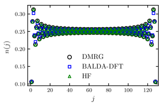
Figure 1: Density profile $n(j)$ for $L=128$ sites and interaction strength $U/t=0.5$ at quarter-filling $\nu=1/4$. Results obtained within the non-self-consistent Hartree-Fock approximation and the BALDA-DFT are compared to “numerically exact” ones computed using DMRG. The DMRG data were provided by C. Karrasch.

In Fig. 1 we compare $n^{\rm HF}(j)$ (and in addition $n^{\rm DFT}(j)$; see Sect. 3.3) with highly accurate (“numerical exact”) results obtained using the density-matrix renormalization group (DMRG). This numerical approach can be used for systems of up to $10^{3}$ lattice sites. In the figure we show data for $L=128$, $\nu=1/4$, and $U/t=0.5$. The overall agreement is acceptable. The data clearly show the $2k_{\rm F}$ periodicity. An analysis of the decay in the light of the asymptotic Tomonaga-Luttinger liquid power law Eq. (7) is meaningless as the overlap of the oscillations originating from the two boundaries of the chain prevents that the asymptotic behavior develops for such small systems. Therefore, larger systems have to be studied.

Using the ${\mathcal{O}}(L)$ algorithm discussed in Sect. 2.4 we can straightforwardly compute $n^{\rm HF}(j)$ for systems of up to $L=10^{6}$ sites. We believe that for a faithful and unbiased search for power-law scaling a corresponding fit of the numerical data is not sufficient. In particular, using perturbation theory we are bound to small interactions, for which the exact exponent is very close to the noninteracting value $-1$; see Eq. (8). In this case a power law might be barely distinguishable from the leading logarithmic behavior analytically found in perturbation theory for the Green function Eq. (21). We will thus perform a more stringent analysis of the data. To this end we focus on the upper envelope of the decaying data (compare Fig. 1), that is the $j$ for which a local maximum is taken. They have a mutual distance of $\nu^{-1}$. We then compute centered logarithmic differences

$$\alpha(j)=\frac{\ln\left[\tilde{n}\left(j+\nu^{-1}\right)\right]-\ln\left[\tilde{n}\left(j-\nu^{-1}\right)\right]}{\ln\left(j+\nu^{-1}\right)-\ln\left(j-\nu^{-1}\right)},$$ (22)

with $\tilde{n}(j)=n(j)-\nu$ , which should approach a constant value (the value of the exponent) for sufficiently large $j$ if the density decays according to a power law. In contrast to a power-law fit the logarithmic differences directly indicate any systematic deviation from power-law behavior. In addition, we compute the following semi-logarithmic centered differences

$$\beta(j)=2\pi\frac{\left(j+\nu^{-1}\right)\tilde{n}\left(j+\nu^{-1}\right)-\left(j-\nu^{-1}\right)\tilde{n}\left(j-\nu^{-1}\right)}{\ln\left(j+\nu^{-1}\right)-\ln\left(j-\nu^{-1}\right)}.$$ (23)

If also the non-self-consistent Hartree-Fock data only show the logarithmic correction Eq. (21) instead of a resummed power law, $\beta(j)$ should display a plateau at the value $\frac{U}{2\pi t\sin(k_{\rm F})}\left[1-\cos\left(2k_{\rm F}\right)\right]$. We then compare $\alpha(j)$ and $\beta(j)$ for a given parameter set to judge which of the two is more plateau-like and thus to judge if the data are more consistent with a power law or the logarithmic behavior Eq. (21). Note that taking the logarithmic differences Eq. (22) or semi-logarithmic ones Eq. (23) significantly enhances any small numerical error in $n(j)$.

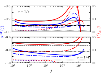
Figure 2: The apparent exponent $\alpha(j)$ Eq. (22) (blue) and the apparent prefactor of $\ln j$ Eq. (23) (red) of the decay of the density oscillations within the non-self-consistent Hartree-Fock approximation for a system with two open boundaries. The parameters are $\nu=1/8$ (upper panel) and $\nu=1/4$ (lower panel), $U/t=0.1$ (dotted), $U/t=0.4$ (dashed-dotted), and $U/t=0.7$ (solid). The horizontal lines indicate the corresponding prefactor of the $\ln j$ term from first order perturbation theory for the Green function Eq. (21). The horizontal dashed line shows this value with $t$ replaced by $\bar{t}$ (only shown for $\nu=1/4$ and $U/t=0.7$).

Figure 3: The same as in Fig. 3, but for a chain with one open boundary, which at $j=L$ is adiabatically connected to a semi-infinite noninteracting lead.

In Fig. 3 we show $\alpha^{\rm HF}(j)$ and $\beta^{\rm HF}(j)$ for $L=2^{20}$, the two fillings $\nu=1/4$ and $\nu=1/8$ as well as three interactions $U/t=0.1$, $U/t=0.4$, and $U/t=0.7$. While for small $U/t$ the numerical non-self-consistent Hartree-Fock data are consistent with both the power law and the logarithmic behavior Eq. (21), for larger $U/t$, $\beta^{\rm HF}(j)$ is more plateau-like as compared to $\alpha^{\rm HF}(j)$. Furthermore, the value of the plateau of $\beta^{\rm HF}(j)$ is close to $\frac{U}{2\pi t\sin(k_{\rm F})}\left[1-\cos\left(2k_{\rm F}\right)\right]$ which is shown as the horizontal lines in Fig. 3. However, due to the effect of the right boundary, at larger $j$ a deviation from the plateau is found already for $j\ll L$.

For $\nu=1/4$ and $U/t=0.7$ a deviation between the plateau value of the data and the expectation (solid horizontal line) from first order perturbation theory is found. This is due to higher order corrections (in $U/t$) appearing in the non-self-consistent Hartree-Fock approximation. For larger interactions those become sizable. One such correction originates from the changed band width $4t\to 4\bar{t}$ as discussed in Sect. 3.1. In fact, in the non-self-consistent Hartree-Fock approximation $t$ is replaced by $\bar{t}$ at any instance the hopping amplitude appears. For this reason the horizontal dashed line (only shown for $\nu=1/4$ and $U/t=0.7$) which indicates $\frac{U}{2\pi\bar{t}\sin(k_{\rm F})}\left[1-\cos\left(2k_{\rm F}\right)\right]$ fits better to the data.

To further investigate $n^{\rm HF}(j)$ we suppress the effect of the right boundary by adiabatically connecting the interacting chain to a semi-infinite noninteracting tight-binding chain at site $j=L$. This way the spatial region $j\approx L$ does not act as a source of any (significant) oscillations in the self-energy and thus not as a source of another decaying oscillation in the density. The technical details how to achieve this are described in Ref. Andergassen04 . In particular, the interaction has to be turned off smoothly over a sufficiently large spatial regime close to $j=L$. Figure 3 shows $\alpha^{\rm HF}(j)$ and $\beta^{\rm HF}(j)$ obtained this way for the same parameters as in Fig. 3. As expected, for most parameter sets the plateau in $\beta^{\rm HF}(j)$ extends towards larger $j$ if the oscillations originating from $j\approx L$ are suppressed. We generically gain between one half and one order of magnitude; compare Figs. 3 and 3. However, our conclusions drawn are the same as the ones from the setup with two open boundaries. Even with a noninteracting lead connected adiabatically deviations from the plateau value are found already at $j<L$. The information about the finiteness of the interacting part of the chain is still encoded in the data.

Based on these results we conclude that the resummation inherent to the Dyson equation (13) does not lead to a resummation of the logarithmic behavior Eq. (21) of first order perturbation theory to a power law. This has to be contrasted to the frequency dependence of the local single-particle spectral function in which this resummation was shown earlier Andergassen04 .

We note in passing, that a self-consistent Hartree-Fock approximation leads to Friedel oscillations with an amplitude which is much larger than the one found using DMRG. Increasing the system size $L$ a nondecaying density oscillation appears to develop; see Ref. Sch and Odavic19 . The self-consistency seemingly triggers a spurious charge-density wave instability. This is not surprising as the 1d system is highly susceptible towards $2k_{\rm F}$ instabilities. The self-consistent Hartree-Fock approximation is thus an inappropriate approach to study the problem at hand.

In our search for an approximate method, which is based on an effective fermionic single-particle picture, to capture the Tomonaga-Luttinger liquid power law Eq. (7), in the next section we use BALDA-DFT. As it is usually the case in a DFT approach the regime of validity given a certain exchange-correlation functional is not obvious a priori. In fact, this is one of our motivations to study the density within BALDA-DFT.

3.3 BALDA-DFT

We finally investigate whether or not the LDA-DFT with an exchange-correlation functional determined from the exact Bethe ansatz solution of the homogeneous system is able to produce the Tomonaga-Luttinger liquid power-law decay of the Friedel density oscillations.

Figure 1 shows $n^{\rm DFT}(j)$ in comparison to $n^{\rm DMRG}(j)$ and $n^{\rm HF}(j)$ for a small system with $L=128$, $\nu=1/4$, and $U/t=0.5$. The BALDA-DFT results are very close to the ones obtained within the non-self-consistent Hartree-Fock approximation.

In Fig. 4 we again consider a larger chain, $L=2^{20}$ and show the logarithmic derivative (the apparent exponent) $\alpha^{\rm DFT}(j)$ for the same parameters as in Fig. 3. Here, we directly study the chain with one open boundary which at $j=L$ is adiabatically connected to a semi-infinite noninteracting lead, a setup which turned out to be advantageous for the analysis of the non-self-consistent Hartree-Fock data. The data show a plateau at intermediate $j$ and are therefore consistent with power-law behavior, however, with an exponent which is far off from the exact one $-K(\nu,U/t)$ (horizontal lines). Based on these results one is tempted to conclude that the BALDA-DFT exponent agrees with the noninteracting value $-1$.

Obviously, the BALDA-DFT does not give a satisfying description of the Tomonaga-Luttinger liquid power-law scaling of the decay of the density away from an open boundary towards the bulk value $\nu$. It, however, does not lead to a spurious charge-density wave instability as found in self-consistent Hartree-Fock. We emphasize that the failure of BALDA-DFT to correctly describe the de- cay of the Friedel oscillations is entirely due to the use of the Bethe ansatz local density approximation. The ex- act functional, which is unknown, would reproduce the many-body density and hence describe the decay of the oscillations correctly.

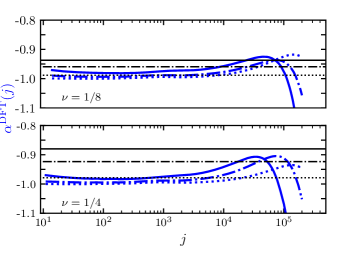
Figure 4: The apparent exponent $\alpha(j)$ Eq. (22) of the decay of the density oscillations within the BALDA-DFT approximation for a chain with one open boundary, which at $j=L$ is adiabatically connected to a semi-infinite noninteracting lead. The parameters are the same as in Fig. 3. Here, the horizontal lines indicate the exact exponent $-K(\nu,U/t)$, with $U/t=0.1$ (dotted), $U/t=0.4$ (dashed-dotted), and $U/t=0.7$ (solid).

4 Conclusion

In this paper we have provided strong numerical evidence that neither the non-self-consistent Hartree-Fock approximation nor a density functional theory approach within the Bethe-ansatz local density approximation are able to capture the Tomonaga-Luttinger liquid power-law decay of the Friedel density oscillations off an open boundary. We focused on the 1d lattice model of spinless fermions with nearest-neighbor hopping and (short-range) nearest-neighbor two-particle interaction.

As expected, first order many-body perturbation theory of the Green function (in the two-particle interaction) shows a logarithmic dependence of the density $n(j)$ on the position which is in accordance with Tomonaga-Luttinger liquid behavior. The numerical data of the non-self-consistent Hartree-Fock approximation indicate that the resummation of higher order terms inherent to the use of the Dyson equation within this approach does not elevate this logarithmic behavior to a power law. The data for the density are rather consistent with $\ln j$ behavior. This has to be contrasted to another observable, the local spectral function close to an open boundary as a function of frequency, for which such a resummation was observed when going from first order perturbation theory for the Green function to the non-self-consistent Hartree-Fock approximation Meden00 . We briefly mentioned that the self-consistent Hartree-Fock approximation is prone to a spurious $2k_{\rm F}$ charge-density wave instability Sch ; Odavic19 .

For the 1d (spinful) Hubbard model the decay of the Friedel density oscillations off an impurity was earlier investigated using BALDA-DFT Lima03 . Even before discussing our BALDA-DFT data for the density, we provided arguments which clearly indicate that the results of Ref. Lima03 were obtained for system sizes which are way to small to allow for a meaningful search for the asymptotic Tomonaga-Luttinger liquid power-law decay. Studying systems of up to $10^{6}$ lattice sites for a spinless model with open boundaries we are in a position to investigate if BALDA-DFT captures this power law. Our numerical data are consistent with a power-law decay of the density oscillations towards the bulk density, however, with the noninteracting exponent $-1$ instead of the interaction and filling dependent one $-K(\nu,U/t)$. We thus conclude that BALDA-DFT does not capture the Tomonaga-Luttinger liquid characteristics of $n(j)$. This result is in accordance with the conclusion reached in Ref. Schenk08 , in which the same model as studied here was investigated. In this paper observables other than the density were computed for systems of a few hundred lattice sites. We reiterate that besides the ground-state energy the density is the observable most directly accessible in a DFT approach. As such one can hope that future improvements to the BALDA functional will be able to describe the decay of the density oscillations correctly.

5 Acknowledgments

This work was supported by the Deutsche Forschungsgemeinschaft via RTG 1995. N.H. acknowledges additional funding from an Emmy-Noether grant of the Deutsche Forschungsgemeinschaft. We thank C. Karrasch for providing the DMRG data of Fig. 1, M. Pletyukhov for discussions on the asymptotic analysis presented in the Appendix, and Nicolai Kitanine for discussions on the Bethe ansatz solution.

Appendix A Details on the perturbation theory for the Green function

In this Appendix, we present details on the asymptotic analysis ($j\rightarrow\infty$) for the Fourier type integrals in Eq. (19). We separately discuss integrals over rectangular and triangular domains, which correspond to the terms that appear in the first and second line of Eq. (20), respectively.

A.1 Integrals over a rectangular domain

Integrals that appear take the following form (for $0<a<b\in\mathbb{R}$)

$$I^{{\rm R}}=\int\limits_{0}^{a}\mathrm{d}x\int\limits_{a}^{b}\mathrm{d}y\frac{\sin{(xj)}\sin{(yj)}}{\cos{(y)}-\cos{(x)}}f(x,y),$$ (24)

where $f(x,y)$ is assumed to be analytic, and symmetric under the exchange of the arguments for the following analysis to apply. These conditions are satisfied by the terms in the first line of Eq. (20). The integrand of Eq. (24) is singular at $x=y=a$. Hence, integration by parts cannot be employed to extract the asymptotics. Therefore, we rewrite the integral as

$$I^{{\rm R}}=\int\limits_{0}^{a}\mathrm{d}x\int\limits_{a}^{b}\mathrm{d}y\Big{(}e^{ixj}-e^{-ixj}\Big{)}\Big{(}e^{iyj}-e^{-iyj}\Big{)}g(x,y),$$ (25)

with $g(x,y)=-\frac{1}{4}\frac{f(x,y)}{\cos{(y)}-\cos{(x)}}$, and proceed by using the method of steepest descent. We deform the integration contour $\mathcal{C}$, which runs from $a$ to $b$ along the real $y$ axis as depicted in Fig. 5 (a), into $\mathcal{C}_{1}\cup\mathcal{C}_{2}\cup\mathcal{C}_{3}\cup\mathcal{C}_{4}\cup\mathcal{C}_{5}\cup\mathcal{C}_{6}$. The integral now reads

$$I^{{\rm R}}=\int\limits_{0}^{\infty}\mathrm{d}(iy)e^{-jy}\int\limits_{0}^{a}\mathrm{d}xh(x)\Big{(}e^{ixj}-e^{-ixj}\Big{)},$$ (26)

with $h(x)=e^{ija}g(x,a+iy)-e^{ijb}g(x,b+iy)+e^{-ija}g(x,a-iy)-e^{-ijb}g(x,b-iy)$. We apply the same steps to the integral over $x$ and deform the contour into three line segments for each of the two terms as before for the integration over $y$.

This time, however, two poles are located on the contour, which arise from the singularity. They were shifted away from the real axis as depicted in Fig. 5 (b). Following this second contour deformation the integral reads

$$I^{{\rm R}}=\int\limits_{0}^{\infty}\mathrm{d}(iy)e^{-yj}\Bigg{\{}i\pi{\rm Res}\Big{[}h(a+ix)e^{ij(a+ix)},x\rightarrow y\Big{]}+i\pi{\rm Res}\Big{[}h(a-ix)e^{-ij(a-ix)},x\rightarrow y\Big{]}$$

$$+\int\limits_{0}^{\infty}\mathrm{d}(ix)e^{-xj}\Big{(}2{\rm Re}\left[h(ix)\right]-e^{ija}h(a+ix)-e^{-ija}h(a-ix)\Big{)}\Bigg{\}},$$ (27)

where ${\rm Res}$ denotes the residue. The poles only contribute with half their residue as they lie on the contour. The integrals in the second line of Eq. (27) are either zero, because the domain of integration is symmetric under reflection with respect to the axis $x=y$, cancel each other under the exchange of arguments, or yield sub-leading contributions $\sim j^{-2}$. The integrals that produce the sub-leading contributions do not contain the pole and can be computed using integration by parts. The leading order contribution to the integral originates from the residues, which when evaluated, give

$$I^{{\rm R}} =\frac{\pi}{4}\int\limits_{0}^{\infty}\mathrm{d}ye^{-2jy}\Bigg{(}\frac{f(a+iy,a+iy)}{\sin{(a+iy)}}e^{2ija}$$

$$+\frac{f(a-iy,a-iy)}{\sin{(a-iy)}}e^{-2ija}\Bigg{)}+\mathcal{O}\big{(}j^{-2}\big{)}.$$ (28)

After substituting $y^{\prime}=jy$ and taking the limit $j\rightarrow\infty$ we obtain the leading order asymptotic contribution as

$$I^{{\rm R}}\approx\frac{\pi}{4j}\frac{f(a,a)}{\sin{(a)}}\cos{(2ja)}.$$ (29)

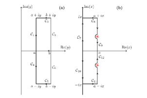
Figure 5: (a) Integration contour of the inner integral. (b) Integration contour of the outer integral. The poles are indicated by the red crosses.

A.2 Integrals over a triangular domain

The integrals we encounter on the triangular domains are of the following form

$$I^{{\rm T}}=\int\limits_{0}^{a}\mathrm{d}x\int\limits_{a}^{2a-x}\mathrm{d}y\frac{\sin{(xj)}\sin{(yj)}}{\cos{(y)}-\cos{(x)}}f(x,y).$$ (30)

The same constraints on $f(x,y)$ as for the integrals on rectangular domains hold. Rewriting the integrand in terms of exponential functions and using the transformation as $(x,y)\mapsto(a-x,a+y)$ we obtain

$$I^{{\rm T}} =\int\limits_{0}^{a}\mathrm{d}x\int\limits_{0}^{x}\mathrm{d}yg(a-x,a+y)\times\Big{(}e^{ij(a-x)}-e^{-ij(a-x)}\Big{)}\times$$

$$\Big{(}e^{ij(a+y)}-e^{-ij(a+y)}\Big{)}.$$ (31)

The transformation shifts the pole from $(a,a)$ to $(0,0)$ and simplifies the computation by fixing the singularity. Using contour extensions for the integral over $y$ we arrive at

$$\tilde{I}^{{\rm T}} =e^{ija}\int\limits_{0}^{a}\mathrm{d}x\int\limits_{0}^{\infty}\mathrm{d}(iy)e^{-jy}$$

$$\times\Bigg{\{}\Big{(}e^{ij(a-x)}-e^{-ij(a-x)}\Big{)}g(a-x,a+iy)$$

$$-\Big{(}e^{ija}-e^{-ij(a-2x)}\Big{)}g(a-x,a+x+iy)\Bigg{\}},$$ (32)

where $I^{{\rm T}}=2{\rm Re}\tilde{I}^{{\rm T}}$. $\tilde{I}^{{\rm T}}$ contains four integrals. Two of those can be evaluated to yield contributions to sub-leading order $\sim j^{-2}$. One contains the pole and computing the residue, as in the case of rectangular integration domains, we obtain to leading order

$$\tilde{I}^{{\rm T}}_{\rm pole}\approx\frac{\pi}{8j\sin{a}}f(a,a)e^{2ija}.$$ (33)

The remaining term reads

$$\frac{e^{2ija}}{4}\int\limits_{0}^{\infty}\mathrm{d}(iy)e^{-jy}\int\limits_{0}^{a}\mathrm{d}x\frac{f(a-x,a+x+iy)}{\cos{(a+x+iy)}-\cos{(a-x)}}.$$ (34)

At this point we need to specify the function $f$ to be able to proceed. As an example, we consider $f(x,y)=\cos{(x+y)}$; see Eq. (20). The integral over $x$ is $j$ independent and can evaluated straightforwardly. It yields

$$-\frac{ie^{2ija}}{8} \int\limits_{0}^{\infty}\mathrm{d}ye^{-jy}\frac{\cos{(2a+iy)}}{\sin{\Big{(}a+\frac{iy}{2}\Big{)}}}$$

$$\times\ln{\Bigg{[}\tan{\Big{(}a/2+iy/4\Big{)}}\cot{\Big{(}iy/4\Big{)}}\Bigg{]}}.$$ (35)

Taking the limit $j\rightarrow\infty$ and using that

$$\int\limits_{0}^{\infty}e^{-xj}\ln{(x)}dx=-\frac{\gamma+\ln{(j)}}{j},$$ (36)

where $\gamma\approx 0.577...$ is the Euler-Mascheroni constant, we obtain a logarithmic contribution to the integral. Combining this with the pole contribution of Eq. (33) we finally obtain for the leading order asymptotics

$$I^{{\rm T}} \approx\frac{\sin{(2ja)}\cos{(2a)}}{4j\sin{(a)}}\Big{\{}\ln{j}+\gamma+\ln{4\tan{(a/2)}}\Big{\}}$$

$$+\frac{\cos{(2ja)}\pi\cos{(2a)}}{8j\sin{(a)}}.$$ (37)

To verify that the analytical expressions Eqs. (29) and (37) for the asymptotic behavior of $I^{{\rm R}}$ and $I^{{\rm T}}$ are indeed correct, we performed numerical integrations for large $j$’s and found agreement. Due to the divergence of the integrand, a particular set of transformations to the integrals needs to be applied before it can reliably be computed numerically. For more details, see Ref. Odavic19 .

Appendix B Authors contributions

All the authors were involved in the preparation of the manuscript. All the authors have read and approved the final manuscript.

References

- (1) K. Schönhammer in Interacting Electrons in Low Dimensions ed. by D. Baeriswyl (Dordrecht: Kluwer Academic Publishers, 2005); arXiv:cond-mat/0305035.
- (2) T. Giamarchi, Quantum Physics in One Dimension (New York: Oxford University Press, 2003).
- (3) F.D.M. Haldane, J. Phys. C 14, 2585 (1981).
- (4) M. Fabrizio and A.O. Gogolin, Phys. Rev. B 51, 17827 (1995).
- (5) R. Egger and H. Grabert, Phys. Rev. Lett. 75, 3505 (1995).
- (6) F.D.M. Haldane, Phys. Rev. Lett. 45, 1358 (1980).
- (7) V. Meden, W. Metzner, U. Schollwöck, O. Schneider, T. Stauber, and K. Schönhammer, Eur. Phys. J. B 16, 631 (2000).
- (8) O. Gunnarsson and K. Schönhammer, Phys. Rev. Lett. 56, 1968 (1986).
- (9) K. Schönhammer, O. Gunnarsson, and R. M. Noack, Phys. Rev. B 52, 2504 (1995).
- (10) N.A. Lima, M.F. Silva, L.N. Oliveira, and K. Capelle, Phys. Rev. Lett. 90, 146402 (2003).
- (11) P. Schmitteckert and F. Evers, Phys. Rev. Lett. 100 086401 (2008).
- (12) P. Hohenberg and W. Kohn, Phys. Rev. 136, B864 (1964).
- (13) S. Schenk, M. Dzierzawa, P. Schwab, and U. Eckern, Phys. Rev. B 78,165102 (2008).
- (14) P. Schmitteckert, Phys. Chem. Chem. Phys. 20, 27600 (2018).
- (15) A. Luther and I. Peschel, Phys. Rev. B 9, 2911 (1974).
- (16) W. Apel and T.M. Rice, Phys. Rev. B 26, 7063 (1982).
- (17) C.L. Kane and M.P.A. Fisher, Phys. Rev. B 46, 15233 (1992).
- (18) S. Andergassen, T. Enss, V. Meden, W. Metzner, U. Schollwöck, and K. Schönhammer, Phys. Rev. B 70, 075102 (2004).
- (19) J. Sólyom, Adv. Phys. 28, 201 (1979).
- (20) S. Andergassen, T. Enss, V. Meden, W. Metzner, U. Schollwöck, and K. Schönhammer, Phys. Rev. B 73, 045125 (2006).
- (21) S. A. Söffing, I. Schneider, and S. Eggert, EPL 101, 56006 (2013).
- (22) N. Kitanine, K.K. Kozlowski, J.M. Maillet, G. Niccoli, N.A. Slavnov, and V. Terras, J. Stat. Mech. P07010 (2008).
- (23) C. Karrasch and J.E. Moore, Phys. Rev. B 86, 155156 (2012).
- (24) L.J. Sham and W. Kohn, Phys. Rev. 145, 561 (1966).
- (25) J. Odavić, PhD Thesis, RWTH Aachen University (2019).
- (26) P. Schmitteckert and U. Eckern, Phys. Rev. B 53, 15397 (1996) .