Is the Policy Gradient a Gradient?

Abstract.

The policy gradient theorem describes the gradient of the expected discounted return with respect to an agent’s policy parameters. However, most policy gradient methods drop the discount factor from the state distribution and therefore do not optimize the discounted objective. What do they optimize instead? This has been an open question for several years, and this lack of theoretical clarity has lead to an abundance of misstatements in the literature. We answer this question by proving that the update direction approximated by most methods is not the gradient of any function. Further, we argue that algorithms that follow this direction are not guaranteed to converge to a “reasonable” fixed point by constructing a counterexample wherein the fixed point is globally pessimal with respect to both the discounted and undiscounted objectives. We motivate this work by surveying the literature and showing that there remains a widespread misunderstanding regarding discounted policy gradient methods, with errors present even in highly-cited papers published at top conferences.

1. Introduction

Reinforcement learning (RL) is a subfield of machine learning in which computational agents learn to maximize a numerical reward signal through interaction with their environment. Policy gradient methods encode an agent’s behavior as a parameterized stochastic policy and update the policy parameters according to an estimate of the gradient of the expected sum of rewards (the expected return) with respect to those parameters. In practice, estimating the effect of a particular action on rewards received far in the future can be difficult, so almost all state-of-the-art implementations instead consider an exponentially discounted sum of rewards (the discounted return), which shortens the effective horizon considered when selecting actions. The policy gradient theorem Sutton et al. (2000) describes the appropriate update direction for this discounted setting. However, almost all modern policy gradient algorithms deviate from the original theorem by dropping one of the two instances of the discount factor that appears in the theorem. It has been an open question for several years as to whether these algorithms are unbiased with respect to a different, related objective Thomas (2014). In this paper, we answer this question and prove that most policy gradient algorithms, including state-of-the-art algorithms, do not follow the gradient of any function. Further, we show that for some tasks, the fixed point of the update direction followed by these algorithms is pessimal, regardless of whether the discounted or undiscounted objective is considered.

The analysis in this paper applies to nearly all state-of-the-art policy gradient methods. In Section 6, we review all of the policy gradient algorithms included in the popular stable-baselines repository Hill et al. (2018) and their associated papers, including A2C/A3C Mnih et al. (2016), ACER Wang et al. (2017), ACKTR Wu et al. (2017), DDPG Lillicrap et al. (2016), PPO Schulman et al. (2017), TD3 Fujimoto et al. (2018), TRPO Schulman et al. (2015a), and SAC Haarnoja et al. (2018). We motivate this choice in Section 6, but we note that all of these papers were published at top conferences and have received hundreds or thousands of citations. We found that all of the implementations of the algorithms used the “incorrect” policy gradient that we discuss in this paper. While this is a valid algorithmic choice if properly acknowledged, we found that only one of the eight papers acknowledged this choice, while three of the papers made erroneous claims regarding the discounted policy gradient and others made claims that were misleading. The purpose of identifying these errors is not to criticize the authors or the algorithms, but to draw attention to the fact that confusion regarding the behavior of policy gradient algorithm exists at the very core of the RL community and has gone largely unnoticed by reviewers. This has led to a proliferation of errors in the literature. We hope that by providing definitive answers to the questions associated with these errors we are able to improve the technical precision of the literature and contribute to the development of a better theoretical understanding of the behavior of reinforcement learning algorithms.

2. Notation

RL agents learn through interactions with an environment. An environment is expressed mathematically as a Markov decision process (MDP). An MDP is a tuple, $(\mathcal{S},\mathcal{A},P,R,d_{0},\gamma)$, where $\mathcal{S}$ is the set of possible states of the environment, $\mathcal{A}$ is the set of actions available to the agent, $P:\mathcal{S}\times\mathcal{A}\times\mathcal{S}\to[0,1]$ is a transition function that determines the probability of transitioning between states given an action, $R:\mathcal{S}\times\mathcal{A}\to[-R_{\text{max}},R_{\text{max}}]$ is the expected reward from taking an action in a particular state, bounded by some $R_{\text{max}}\in\mathbb{R}$, $d_{0}:\mathcal{S}\to[0,1]$ is the initial state distribution, and $\gamma\in[0,1]$ is the discount factor which decreases the utility of rewards received in the future. In the episodic setting, interactions with the environment are broken into independent episodes. Each episode is further broken into individual timesteps. At each timestep, $t$, the agent observes a state, $S_{t}$, takes an action, $A_{t}$, transitions to a new state, $S_{t+1}$, and receives a reward, $R_{t}$. Each episode begins with $t=0$ and ends when the agent enters a special state called the terminal absorbing state, $s_{\infty}$. Once $s_{\infty}$ is entered, the agent can never leave and receives a reward of 0 forever. We assume that $\lim_{t\to\infty}\Pr(S_{t}=s_{\infty})=1$, since otherwise, the episode may persist indefinitely and the continuing setting must be considered.

A policy, $\pi:\mathcal{S}\times\mathcal{A}\to[0,1]$, determines the probability that an agent will choose an action in a particular state. A parameterized policy, $\pi^{\theta}$, is a policy that is defined as a function of some parameter vector, $\theta$, which may be the weights in a neural network, values in a tabular representation, etc. The compatible features of a parameterized policy represent how $\theta$ may be changed in order to make a particular action, $a\in\mathcal{A}$, more likely in a particular state, $s\in\mathcal{S}$, and are defined as $\psi(s,a)\coloneqq\frac{\partial}{\partial\theta}\ln\pi^{\theta}(s,a)$. The value function, $V^{\theta}_{\gamma}:\mathcal{S}\to\mathbb{R}$, represents the expected discounted sum of rewards when starting in a particular state under policy $\pi^{\theta}$; that is, $\forall t,V^{\theta}_{\gamma}(s)\coloneqq\mathbb{E}[\sum_{k=0}^{\infty}\gamma^{k}R_{t+k}|S_{t}{=}s,\theta]$, where conditioning on $\theta$ indicates that $\forall t,A_{t}\sim\pi^{\theta}(S_{t},\cdot)$. The action-value function, $Q^{\theta}_{\gamma}:\mathcal{S}\times\mathcal{A}\to\mathbb{R}$, is similar, but also considers the action taken; that is, $\forall t,Q^{\theta}_{\gamma}(s,a)\coloneqq\mathbb{E}[\sum_{k=0}^{\infty}\gamma^{k}R_{t+k}|S_{t}{=}s,A_{t}{=}a,\theta]$. The advantage function is the difference between the action-value function and the (state) value function: $A^{\theta}_{\gamma}(s,a)\coloneqq Q^{\theta}_{\gamma}(s,a)-V^{\theta}_{\gamma}(s)$.

The objective of an RL agent is to maximize some function, $J$, of its policy parameters, $\theta$. In the episodic setting, the two most commonly stated objectives are the discounted objective, $J_{\gamma}(\theta)=\mathbb{E}[\sum_{t=0}^{\infty}\gamma^{t}R_{t}|\theta]$, and the undiscounted objective, $J(\theta){=}\mathbb{E}[\sum_{t=0}^{\infty}R_{t}|\theta]$. The discounted objective has some convenient mathematical properties, but it corresponds to few real-world tasks. Sutton and Barto (2018) have even argued for its deprecation. However, we will see in Section 6 that the discounted objective is commonly stated as a justification for the use of a discounted factor, even when the algorithms themselves do not optimize this objective.

3. Problem Statement

The formulation of the policy gradient theorem Williams (1992); Sutton et al. (2000); Baxter and Bartlett (2000) presented by Sutton et al. (2000) was given for two objectives: the average reward objective for the infinite horizon setting Mahadevan (1996) and the discounted objective, $J_{\gamma}$, for the episodic setting. The episodic setting considered in this paper is more popular, as it is better suited to the types of tasks that RL researchers typically use for evaluation (e.g., many classic control tasks, Atari games Bellemare et al. (2013), etc.). The discounted policy gradient, $\nabla J_{\gamma}(\theta)$, tells us how to modify the policy parameters, $\theta$, in order to increase $J_{\gamma}$, and is given by:

$$\nabla J_{\gamma}(\theta)=\mathbb{E}\left[\sum_{t=0}^{\infty}\gamma^{t}\psi^{\theta}(S_{t},A_{t})Q^{\theta}_{\gamma}(S_{t},A_{t})\bigg{|}\theta\right].$$ (1)

Because $\nabla J_{\gamma}$ is the true gradient of the discounted objective, algorithms that follow unbiased estimates of it are given the standard guarantees of stochastic gradient descent (namely, that given an appropriate step-size schedule and smoothness assumptions, convergence to a locally optimal policy is almost sure Bertsekas and Tsitsiklis (2000)). However, most conventional “policy gradient” algorithms instead directly or indirectly estimate the expression:

$$\nabla J_{?}(\theta)=\mathbb{E}\left[\sum_{t=0}^{\infty}\psi^{\theta}(S_{t},A_{t})Q^{\theta}_{\gamma}(S_{t},A_{t})\bigg{|}\theta\right].$$ (2)

Note that this expression includes the $\gamma^{t}$ contained in $Q^{\theta}_{\gamma}$, but differs from the true discounted policy gradient in that it drops the outer $\gamma^{t}$. We label this expression $\nabla J_{?}(\theta)$ because the question of whether or not it is the gradient of some objective function, $J_{?}$, was left open by Thomas (2014). Thomas (2014) was only able to construct $J_{?}$ in an impractically restricted setting where $\pi$ did not affect the state distribution. The goal of this paper is to provide answers to the following questions:

• Is $\nabla J_{?}(\theta)$ the gradient of some objective function?

• If not, does $\nabla J_{?}(\theta)$ at least converge to a reasonable policy?

4. $\nabla J_{?}(\theta)$ is Not a Gradient

In this section, we answer the first of our two questions and show that the update direction used by almost all policy gradient algorithms, $\nabla J_{?}(\theta)$, is not the gradient of any function using a proof by contraposition with the Clairaut-Schwarz theorem on mixed partial derivatives Schwarz (1873). First, we present this theorem (Theorem 4) and its contrapositive (Corollary 4). Next, we present Lemma 4, which allows us to rewrite $\nabla J_{?}(\theta)$ in a new form. Finally, in Theorem 4 we apply Corollary 4 and Lemma 4 and derive a counterexample proving that $J_{?}$ does not, in general, exist, and therefore that the “policy gradient” given by $\nabla J_{?}(\theta)$ is not, in fact, a gradient.

(Clairaut-Schwarz theorem): If $f:\mathbb{R}^{n}\to\mathbb{R}$ exists and is continuously twice differentiable in some neighborhood of the point $(a_{1},a_{2},\dots,a_{n})$, then its second derivative is symmetric:

$$\forall i,j:\frac{\partial f(a_{1},a_{2},\dots,a_{n})}{\partial x_{i}\partial x_{j}}=\frac{\partial f(a_{1},a_{2},\dots,a_{n})}{\partial x_{j}\partial x_{i}}.$$ (3)

Proof.

The first complete proof was given by Schwarz Schwarz (1873). English proofs can be found in many advanced calculus and analysis textbooks (Rudin et al., 1964, p. 236). ∎

Corollary

(Contrapositive of Clairaut-Shwarz): If at some point $(a_{1},a_{2},\dots,a_{n})$ $\in\mathbb{R}^{n}$ there exists an $i$ and $j$ such that

$$\frac{\partial f(a_{1},a_{2},\dots,a_{n})}{\partial x_{i}\partial x_{j}}\neq\frac{\partial f(a_{1},a_{2},\dots,a_{n})}{\partial x_{j}\partial x_{i}},$$ (4)

then $f$ does not exist or is not continuously twice differentiable in any neighborhood of $(a_{1},a_{2},\dots,a_{n})$.

Proof.

Contrapositive of Theorem 4. As a reminder, the contrapositive of a statement, $P\implies Q$, is $\neg Q\implies\neg P$. The contrapositive is always implied by the original statement. Additionally, recall that for any function $g$, $\neg\forall i:g(i)\implies\exists i:\neg g(i)$. ∎

If we can find an example where $\nabla^{2}J_{?}(\theta)$ is continuous but asymmetric, that is, $\exists i,j:\frac{\partial J_{?}(\theta)}{\partial\theta_{i}\partial\theta_{j}}\neq\frac{\partial J_{?}(\theta)}{\partial\theta_{j}\partial\theta_{i}}$, then we may apply Corollary 4 and conclude that $J_{?}$ does not exist. To this end, we present a new lemma that allows us to rewrite $\nabla J_{?}(\theta)$ in a form that is more amenable to computing the second derivatives by hand. The result of this lemma is of some theoretical interest in itself, but further interpretation is left as future work. We do not leverage it here for any purpose except to aid in our proof of Theorem 4.

Lemma

Let $d^{\theta}_{\gamma}$ be the unnormalized, weighted state distribution given by:

$$d^{\theta}_{\gamma}(s)\coloneqq d_{0}(s)+(1-\gamma)\sum_{t=1}^{\infty}\Pr(S_{t}=s|\theta).$$ (5)

Then:

$$\nabla J_{?}(\theta)=\sum_{s\in\mathcal{S}}d^{\theta}_{\gamma}(s)\frac{\partial}{\partial\theta}V^{\theta}_{\gamma}(s).$$ (6)

Proof.

See appendix. ∎

In this form, we begin to see the root of the issue: In the above expression, $d^{\theta}_{\gamma}(s)$ is not differentiated, meaning that $\nabla J_{?}(\theta)$ does not consider the effect updates to $\theta$ have on the state distribution. We will show that this is in fact the source of the asymmetry in $\nabla^{2}J_{?}(\theta)$. With this in mind, we present our main theorem.

Let $\mathcal{M}$ be the set of all MDPs with rewards bounded by $[-R_{\text{max}},R_{\text{max}}]$ satisfying $\forall\pi:\sum_{t=0}^{\infty}\Pr(S_{t}\neq s_{\infty})<\infty$. Then, for all $\gamma<1$:

$$\neg\exists J_{?}:\forall M{\in}\mathcal{M}:\nabla J_{?}(\theta)=\mathbb{E}\left[\sum_{t=0}^{\infty}\psi^{\theta}(S_{t},A_{t})Q^{\theta}_{\gamma}(S_{t},A_{t})\middle|\theta\right].$$

Proof.

Theorem 4 states that if $J_{?}$ is a twice continuously differentiable function, then its second derivative is symmetric. It is easy to show that this is not true informally using Lemma 4:

$$\frac{\partial^{2}J_{?}(\theta)}{\partial\theta_{i}\partial\theta_{j}} =\frac{\partial}{\partial\theta_{i}}\left(\sum_{s\in\mathcal{S}}d^{\theta}_{\gamma}(s)\frac{\partial}{\partial\theta_{j}}V^{\theta}_{\gamma}(s)\right)$$

$$=\underbrace{\sum_{s\in\mathcal{S}}d^{\theta}_{\gamma}(s)\frac{\partial^{2}}{\partial\theta_{i}\partial\theta_{j}}V^{\theta}_{\gamma}(s)}_{\text{symmetric}}+\underbrace{\sum_{s\in\mathcal{S}}\frac{\partial}{\partial\theta_{i}}d^{\theta}_{\gamma}(s)\frac{\partial}{\partial\theta_{j}}V^{\theta}_{\gamma}(s)}_{\text{asymmetric}}.$$

Therefore, we have by Corollary 4 that so long as $\nabla^{2}J_{?}(\theta)$ is continuous, $J_{?}$ does not exist. In order to rigorously complete the proof, we must provide as a counterexample an MDP for which the above asymmetry is present. We provide such a counterexample in Figure 1. While we defer the full proof to the appendix, we describe the intuition behind the counterexample below.

Assume that for the example given in Figure 1, $J_{?}$ exists and $\nabla J_{?}(\theta)$ is its gradient. Consider in particular the case where $\gamma=0$. In this case, $\nabla^{2}J_{?}(\theta)$ is asymmetric because $\theta_{1}$ affects the value function and the state distribution, whereas $\theta_{2}$ affects the value function but not the state distribution. Therefore, the second term in $\partial^{2}J_{?}(\theta)/\partial\theta_{i}\partial\theta_{j}$ (labeled “asymmetric” in the above equation) is non-zero when $i=1$ and $j=2$, and zero when $i=2$ and $j=1$. In the appendix, we show that the above expression is symmetric if and only if $\gamma=1$. Therefore, for $\gamma<1$, Corollary 4 applies and we may conclude that $J_{?}$ either does not exist or is not continuously twice differentiable. In this example, the $\nabla^{2}J_{?}(\theta)$ is continuous everywhere. Therefore, we conclude that $J_{?}$ does not exist. This completes the counterexample.

∎

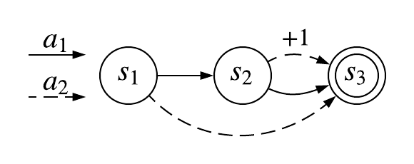
Figure 1. A counterexample wherein the derivative of $\nabla J_{?}(\theta)$ is asymmetric for all $\gamma<1$, necessary for the proof of Theorem 4. The agent begins in $s_{1}$, and may choose between actions $a_{1}$ and $a_{2}$, each of which produces deterministic transitions. The rewards are 0 everywhere except when the agent chooses $a_{2}$ in state $s_{2}$, which produces a reward of $+1$. The policy is assumed to be tabular over states and actions, with one parameter, $\theta_{1}$, determining the policy in $s_{1}$, and a second parameter, $\theta_{2}$, determining the policy in $s_{2}$ (e.g., the policy may be determined by the standard logistic function, $\sigma(x)=\frac{1}{1+e^{-x}}$, such that $\pi(s_{1},a_{1})=\sigma(\theta_{1})$).

5. The Fixed Point of $\nabla J_{?}(\theta)$ is Sometimes Pessimal

Having established that $\nabla J_{?}(\theta)$ is not the gradient of any function for choices of $\gamma<1$, we move on to the question of whether or not $\nabla J_{?}(\theta)$ converges to some reasonable policy in the general case. For instance, consider the case of temporal difference (TD) methods. While the expected update of TD is not a gradient update Sutton (2015), in the on-policy setting with a linear function approximator, TD has been shown to converge to a unique point close to the global optimum of the mean-squared projected Bellman error (MSPBE) Tsitsiklis and Van Roy (1997); Sutton et al. (2009); Sutton and Barto (2018), which is called the “TD fixed point.” Through the geometric interpretation of the MSPBE, it may be said that the TD fixed point is “reasonable” in that it is close to the best possible estimate of the mean squared Bellman error (MSBE) under a particular linear parameterization of the value function.

We ask the question of whether or not a similar reasonable fixed point exists in the case of the update given by $\nabla J_{?}(\theta)$. While it is not clear in what sense the fixed point should be “reasonable,” we propose a very minimal criterion: any reasonable policy fixed point should at least surpass the worst possible (pessimal) policy under either the discounted or undiscounted objective. That is, if the fixed point is pessimal under both objectives, this suggests that it will be difficult to come up with a satisfactory justification. Surprisingly, it can be shown that $\nabla J_{?}(\theta)$ fails to pass even this low bar.

To demonstrate this, we contrast two examples, given in Figures 3 and 3. In the former example, $\nabla J_{?}(\theta)$ behaves in a way that is (perhaps) expected: it converges to the optimal policy under the discounted objective, while failing to optimize the undiscounted objective. This is a well understood trade-off of discounting that can be explained as “short-sightedness” by the agent. The latter example, however, shows a case where an agent following $\nabla J_{?}(\theta)$ behaves in a manner that is apparently irrational: it achieves the smallest possible discounted return and undiscounted return, despite the fact that it is possible to maximize either within the given policy parameterization. We therefore suggest that for at least some MDPs, $\nabla J_{?}(\theta)$ may not be a reasonable choice.

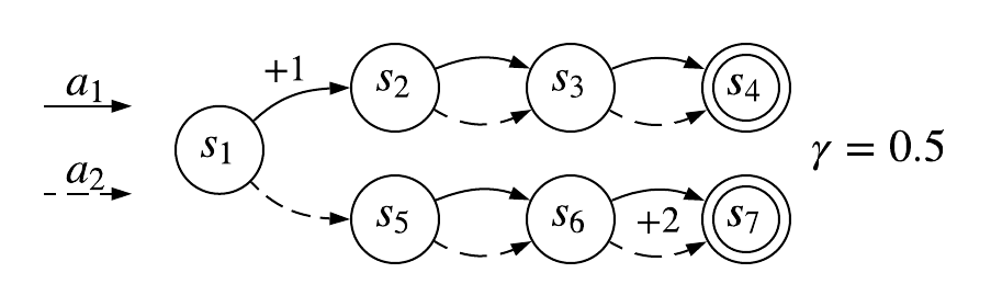
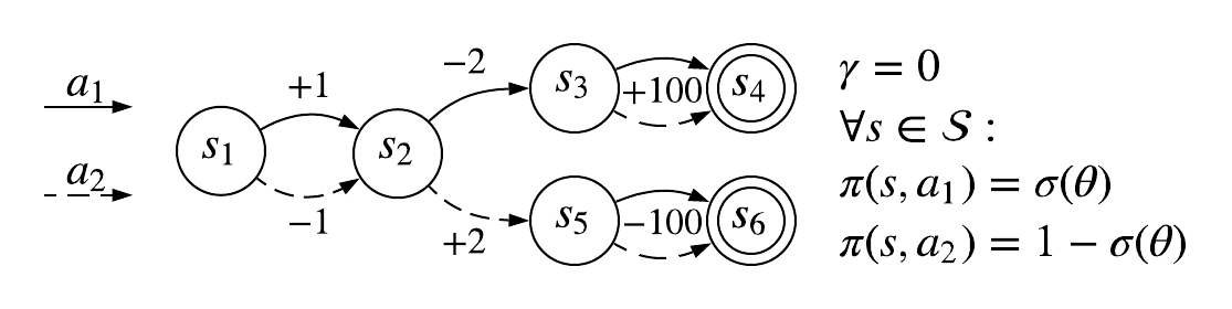
Figure 2. An example where the fixed point of $\nabla J_{?}(\theta)$ is optimal with respect to the discounted objective but pessimal with respect to the undiscounted objective. The agent starts in state $s_{1}$, and can achieve a reward of $+1$ by transitioning from $s_{1}$ to $s_{2}$, and a reward of $+2$ by transitioning from $s_{6}$ to $s_{7}$, regardless of the action taken. In order to maximize the undiscounted return, the agent should choose $a_{2}$. However, the discounted return is higher from choosing $a_{1}$. Only the return in $s_{1}$ will affect the policy gradient as the advantage is zero in every other state. Thus, algorithms following $\nabla J_{?}(\theta)$ methods will eventually choose $a_{1}$. If the researcher is concerned with the undiscounted objective, as is often the case, this result is problematic. Choosing a larger value of $\gamma$ trivially fixes the problem in this particular example, but for any value of $\gamma<1$, similar problems will arise given a sufficiently long horizon, and thus the problem is not truly eliminated. Nevertheless, this is well-understood as the trade-off of discounting.

Figure 3. An example where the fixed point of $\nabla J_{?}(\theta)$ is pessimal with respect to both the discounted and undiscounted objectives. In this formulation, there is a single policy parameter, $\theta$, so the agent must execute the same policy in every state. It is difficult to justify any solution other than to always choose $a_{1}$. If the agent is completely myopic, then $a_{1}$ gives the superior immediate reward of $+1$ in the starting state. If the agent is somewhat farther-sighted, then always choosing $a_{1}$ will eventually result in the $+100$ reward. Choosing $a_{2}$ provides no benefit with respect to either view. Following $\nabla J_{?}(\theta)$, however, will result in a policy that always chooses $a_{2}$. This results from the fact that the advantage of $a_{2}$ in state $s_{2}$ is greater than the advantage of $a_{1}$ in state $s_{1}$, while the advantages in states $s_{3}$ and $s_{5}$ are zero. Because $\nabla J_{?}(\theta)$ ignores the change in the state distribution, the net update always increases the probability of choosing $a_{2}$. Again, while we chose $\gamma=0$ for simplicity, similar examples can be produced in long-horizon problems with “reasonable” settings of $\gamma$, such as $0.99$ or higher. One may ask if the sharing of a policy between states is contrived, but such a situation occurs reliably under partial observability or when a function approximator is used.

6. Literature Review

We previously claimed that $\nabla J_{?}(\theta)$ is the direction followed by state-of-the-art policy gradient methods and that the lack of theoretical clarity on the behavior of algorithms following $\nabla J_{?}(\theta)$ has resulted in a multiplicity of errors in the literature. In this section, we substantiate this point by surveying a subset of popular policy gradient algorithms and their associated papers. We show that the majority of them include erroneous or misleading statements directly relating to arguments made in this paper. We emphasize that we do not pose this as a criticism of the authors, but rather a symptom of the ambiguity in the literature that we hope to address with this paper.

6.1. Methodology

Rather than manually selecting which papers to review, which may have introduced an unacceptable degree of bias, we chose to review the papers associated with every policy gradient algorithm included in stable-baselines Hill et al. (2018), a fork of the popular OpenAI baselines Dhariwal et al. (2017) library. We chose this particular subset of algorithms because inclusion in the library generally indicates that the algorithms have achieved a certain level of popularity and relevance. The papers corresponding to these algorithms have received hundreds or thousands of citations each, and, with the exception of PPO Schulman et al. (2017), were published at top machine learning conferences. It therefore seems reasonable to claim that the papers were impactful in the field and are representative of high-quality research. While we acknowledge that this sampling of algorithms is heavily biased towards the subfield of “deep” RL, we argue that this is not unreasonable given the immense popularity of this area and its impact on the broader field.

For each algorithm, we examined the psuedocode for the algorithm itself, the background and theoretical sections of the associated paper, and several publicly available implementations, including the implementation created by the authors where available. We tried to answer the following three questions for each algorithm:

1. Does the algorithm use $\nabla J_{?}(\theta)$ rather than an unbiased estimator?

2. If so, did the authors note that $\nabla J_{?}(\theta)$ is not an unbiased estimator of the policy gradient?

3. Did the paper include any erroneous or misleading claims about $\nabla J_{?}(\theta)$?

For questions (2) and (3), we support our evaluation of the papers with quotations from the text in cases where there were errors or ambiguities. While this approach is verbose, we felt that paraphrasing the original papers would not allow the readers understand the errors in their appropriate context. For 5 out of 8 of the algorithms, the original authors or organizations provided code, allowing us to directly answer (1). For all eight papers, we examined the stable-baselines Hill et al. (2018) implementation as well as several other implementations including tf-agents Sergio Guadarrama, Anoop Korattikara, Oscar Ramirez, Pablo Castro, Ethan Holly, Sam Fishman, Ke Wang, Ekaterina Gonina, Neal Wu, Efi Kokiopoulou, Luciano Sbaiz, Jamie Smith, Gábor Bartók, Jesse Berent, Chris Harris, Vincent Vanhoucke, Eugene Brevdo (2018), garage garage contributors (2019), spinning-up Achiam (2018), and the autonomous-learning-library Nota (2020). Finally, for each paper we note the conference, year, and citation count estimated by Google Scholar on February 23, 2020.

6.2. Results

Eight policy gradient algorithms are included in stable-baselines. Our high-level results to each question are as follows:

1. All eight of the algorithms use $\nabla J_{?}(\theta)$ instead of an unbiased estimator, both in their psuedocode and implementations.

2. Only one out of the eight papers calls attention to the fact that $\nabla J_{?}(\theta)$ is a biased estimator.

3. Three out of the eight papers included claims that are clearly erroneous. Two additional papers made misleading claims in that they presented the discounted policy gradient ($\nabla J_{\gamma}(\theta)$), and then proposed an algorithm that uses $\nabla J_{?}(\theta)$, without making note of this discrepancy. A sixth paper included claims that we argue are misleading, but not strictly false.

We reproduce the three explicitly erroneous claims below in order to give the reader a sense of common misunderstandings. Notice that the quotations sometimes use slightly different notation than this paper. We try to supply the appropriate context such that the meaning intended by the authors can be understood. Additional analysis can be found in the appendix.

A3C (ICML 2016, 2859 citations)

Asynchronous Advantage Actor-Critic (A3C) Mnih et al. (2016) is an actor-critic method that generates sample batches by running multiple actors in parallel. The original version of the algorithm achieved state-of-the-art performance on many Atari games when it was published. The background section of the main paper includes the text:

The return $R_{t}=\sum_{k=0}^{\infty}\gamma^{k}r_{t+k}$ is the total accumulated return from time step $t$ with discount factor $\gamma\in(0,1]$. The goal of the agent is to maximize the expected return from each state $s_{t}$.

[…]

In contrast to value-based methods, policy based methods directly parameterize the policy $\pi(a|s;\theta)$ and update the parameters $\theta$ by performing, typically approximate, gradient ascent on $\mathbb{E}[R_{t}]$. One example of such a method is the REINFORCE family of algorithms due to Williams (1992). Standard REINFORCE updates the policy parameters $\theta$ in the direction $\nabla_{\theta}\log\pi(a_{t}|s_{t};\theta)R_{t}$, which is an unbiased estimate of $\nabla_{\theta}\mathbb{E}[R_{t}]$. It is possible to reduce the variance of this estimate while keeping unbiased by subtracting a learned function of the state $b_{t}(s_{t})$, known as a baseline Williams (1992), from the return. The resulting gradient is $\nabla_{\theta}\log(a_{t}|s_{t};\theta)(R_{t}-b_{t}(s_{t}))$.

It is falsely claimed that $\nabla_{\theta}\pi(a_{t}|s_{t};\theta)R_{t}$ (which is an unbiased sample estimate of $\nabla J_{?}(\theta)$) is an unbiased estimate of $\nabla_{\theta}\mathbb{E}[R_{t}]$, where $R_{t}$ is the discounted return at timestep $t$ rather than the individual reward. We showed that this is not the case.

ACKTR (ICLR 2017, 235 citations)

Actor Critic using Kronecker-Factored Trust Region (ACKTR) Wu et al. (2017) is a variation of A3C that attempts to efficiently estimate the natural policy gradient, which uses an alternate notion of the direction of steepest ascent. The resulting algorithm is considerably more sample efficient than A3C. The background section contains:

The goal of the agent is to maximize the expected $\gamma$-discounted cumulative return $J(\theta)=\mathbb{E}_{\pi}[R_{t}]=\mathbb{E}_{\pi}[\sum_{i\geq 0}^{\infty}\gamma^{i}r(s_{t+i},a_{t+i})]$ with respect to the policy parameters $\theta$. Policy gradient methods directly parameterize a policy $\pi_{\theta}(a|s_{t})$ and update parameter $\theta$ so as to maximize the objective $J(\theta)$. In its general form Schulman et al. (2015b), the policy gradient is defined as:

$$\nabla_{\theta}J(\theta)=\mathbb{E}_{\pi}\left[\sum_{t=0}^{\infty}\Psi^{t}\nabla_{\theta}\log\pi_{\theta}(a_{t}|s_{t})\right],$$ (7)

where $\Psi^{t}$ is often chosen to be the advantage function $A^{\pi}(s_{t},a_{t})$, which provides a relative measure of value of each action $a_{t}$ at a given state $s_{t}$.

The authors assert that the gradient, $\nabla_{\theta}J(\theta)$, is equal to the given expression, which is false for the proposed choice of $A^{\pi}(s_{t},a_{t})$. They did not note that above expression is an approximation or otherwise clarify. Therefore, the definition of the policy gradient presented above is erroneous.

SAC (ICML 2018, 446 citations)

Soft Actor-Critic (SAC) Haarnoja et al. (2018) is an algorithm in the deterministic policy gradient family Silver et al. (2014). The deterministic policy gradient gives an expression for updating the parameters of a deterministic policy and is derived from the conventional policy gradient theorem, meaning that the arguments presented in this paper apply. SAC is considered state-of-the-art on continuous control tasks. The appendix states:

The exact definition of the discounted maximum entropy objective is complicated by the fact that, when using a discount factor for policy gradient methods, we typically do not discount the state distribution, only the rewards. In that sense, discounted policy gradients typically do not optimize the true discounted objective. Instead, they optimize average reward, with the discount serving to reduce variance, as discussed by Thomas (2014).

The relationship between the average reward objective and $\nabla J_{?}(\theta)$ was discussed by Kakade (2001) and elaborated on by Thomas (2014). However, the claim that $\nabla J_{?}(\theta)$ optimizes the average reward objective is erroneous by Theorem 4.

6.3. Discussion

The three erroneous claims all involved misinterpreting $\nabla J_{?}(\theta)$ as the gradient of some function. Two of the remaining papers failed to acknowledge the difference between the gradient of the discounted objective, $\nabla J_{\gamma}(\theta)$, and the gradient direction followed by the presented algorithm, typically an estimate of $\nabla J_{?}(\theta)$. Even among the papers where we did not find explicit errors, errors were avoided largely through the use of hedged language and ambiguity, rather than technical precision. For examples of this, we encourage the reader to refer to the appendix. While for the purposes of this review we only sampled a small subset of the literature on policy gradients, we found the results sufficient to support our claim that there exists a widespread misunderstanding regarding $\nabla J_{?}(\theta)$.

7. Conclusions

We conclude by emphasizing the while $\nabla J_{?}(\theta)$ is not a gradient (Section 4), can in some cases result in pessimal behavior (Section 5), and is commonly misrepresented in the literature (Section 6), it has remained the most popular estimator of the policy gradient due to its effectiveness when applied to practical problems. The precise reason for this effectiveness, especially in the episodic setting, remains an open question.

Appendix

Proof of Lemma 4.1

We begin by hypothesizing that $\nabla J_{?}(\theta)$ takes the form of a weighted distribution over $\frac{\partial}{\partial\theta}V^{\theta}_{\gamma}(s)$, given some time-dependent weights, $w(t)$, on each term in the state distribution. That is, we hypothesize that equality:

$$\nabla J_{?}(\theta)=\sum_{s\in\mathcal{S}}d^{\theta}_{\gamma}(s)\frac{\partial}{\partial\theta}V^{\theta}_{\gamma}(s),$$ (8)

holds for some $d^{\theta}_{\gamma}$:

$$d^{\theta}_{\gamma}(s)=\sum_{t=0}^{\infty}w(t)\Pr(S_{t}=s|\theta).$$

We then must prove that this holds for some choice of $w(t)$, and then derive the satisfying choice of $w(t)$. Sutton et al. (2000) established that:

$$\frac{\partial}{\partial\theta}V^{\theta}_{\gamma}(s){=}\sum_{k=0}^{\infty}\sum_{x\in\mathcal{S}}\gamma^{k}\Pr(S_{t+k}{=}x|S_{t}{=}s,\theta)\sum_{a\in\mathcal{A}}Q^{\theta}_{\gamma}(x,a)\frac{\partial\pi^{\theta}(x,a)}{\partial\theta}.$$ (9)

Substituting this into our expression for $\nabla J_{?}(\theta)$ gives us:

$$\sum_{s\in\mathcal{S}}d^{\theta}_{\gamma}(s)\frac{\partial}{\partial\theta}V^{\theta}_{\gamma}(s)$$

$$= \sum_{s\in\mathcal{S}}\sum_{t=0}^{\infty}w(t)\Pr(S_{t}=s|\theta)$$

$$\times\sum_{k=0}^{\infty}\sum_{x\in\mathcal{S}}\gamma^{k}\Pr(S_{t+k}=x|S_{t}=s,\theta)\sum_{a\in\mathcal{A}}Q^{\theta}_{\gamma}(x,a)\frac{\partial\pi^{\theta}(x,a)}{\partial\theta}$$

$$= \sum_{s\in\mathcal{S}}\sum_{t=0}^{\infty}\sum_{k=0}^{\infty}\sum_{x\in\mathcal{S}}\sum_{a\in\mathcal{A}}w(t)\gamma^{k}$$

$$\times\Pr(S_{t}=s|\theta)\Pr(S_{t+k}=x|S_{t}=s,\theta)Q^{\theta}_{\gamma}(x,a)\frac{\partial\pi^{\theta}(x,a)}{\partial\theta}$$

$$= \sum_{s\in\mathcal{S}}\sum_{t=0}^{\infty}\sum_{k=0}^{\infty}\sum_{x\in\mathcal{S}}\sum_{a\in\mathcal{A}}w(t)\gamma^{k}$$

$$\times\Pr(S_{t}=s|\theta)\Pr(S_{t+k}=x|S_{t}=s,\theta)Q^{\theta}_{\gamma}(x,a)\pi^{\theta}(x,a)\frac{\partial\ln(\pi^{\theta}(x,a))}{\partial\theta}$$

$$= \sum_{s\in\mathcal{S}}\sum_{t=0}^{\infty}\sum_{k=0}^{\infty}\sum_{x\in\mathcal{S}}\sum_{a\in\mathcal{A}}w(t)\gamma^{k}$$

$$\times\Pr(S_{t}=s|\theta)\Pr(S_{t+k}=x|S_{t}=s,\theta)Q^{\theta}_{\gamma}(x,a)\pi^{\theta}(x,a)\psi(x,a)$$

$$= \sum_{s\in\mathcal{S}}\sum_{t=0}^{\infty}\sum_{k=0}^{\infty}\sum_{x\in\mathcal{S}}\sum_{a\in\mathcal{A}}w(t)\gamma^{k}$$

$$\times\Pr(S_{t}=s|\theta)\Pr(S_{t+k}=x|S_{t}=s,\theta)\Pr(A_{t+k}=a|S_{t+k}=x,\theta)$$

$$\times Q^{\theta}_{\gamma}(x,a)\psi(x,a)$$

$$= \sum_{t=0}^{\infty}\sum_{k=0}^{\infty}\sum_{x\in\mathcal{S}}\sum_{a\in\mathcal{A}}w(t)\gamma^{k}$$

$$\times\Pr(S_{t+k}=x|\theta)\Pr(A_{t+k}=a|S_{t+k}=x,\theta)Q^{\theta}_{\gamma}(x,a)\psi(x,a),$$

since $\Pr(A_{t+k}=a|S_{t+k}=x,\theta)=\Pr(A_{t+k}=a|S_{t+k}=x,S_{t}=s,\theta)$ and by the law of total probability. The key point is that we have removed the term $\Pr(S_{t}=s|\theta)$. Continuing, starting with the fact that $\Pr(S_{t+k}=x|\theta)\Pr(A_{t+k}=a|S_{t+k}=x,\theta)=\Pr(S_{t+k}=x,A_{t+k}=a|\theta)$, we have that:

$$\sum_{s\in\mathcal{S}}d^{\theta}_{\gamma}(s)\frac{\partial}{\partial\theta}V^{\theta}_{\gamma}(s)$$

$$= \sum_{t=0}^{\infty}\sum_{k=0}^{\infty}\sum_{x\in\mathcal{S}}\sum_{a\in\mathcal{A}}w(t)\gamma^{k}\Pr(S_{t+k}=x,A_{t+k}=a|\theta)Q^{\theta}_{\gamma}(x,a)\psi(x,a)$$

$$= \sum_{t=0}^{\infty}\sum_{k=0}^{\infty}\mathbb{E}\left[w(t)\gamma^{k}Q^{\theta}_{\gamma}(S_{t+k},A_{t+k})\psi(S_{t+k},A_{t+k})\middle|\theta\right]$$

$$= \sum_{t=0}^{\infty}\sum_{i=t}^{\infty}\mathbb{E}\left[w(t)\gamma^{i-t}Q^{\theta}_{\gamma}(S_{i},A_{i})\psi(S_{i},A_{i})\middle|\theta\right],$$

by substitution of the variable $i=t+k$. Continuing, we can move the summation inside the expectation and reorder the summation:

$$\sum_{s\in\mathcal{S}}d^{\theta}_{\gamma}(s)\frac{\partial}{\partial\theta}V^{\theta}_{\gamma}(s) =\mathbb{E}\left[\sum_{t=0}^{\infty}\sum_{i=t}^{\infty}w(t)\gamma^{i-t}Q^{\theta}_{\gamma}(S_{i},A_{i})\psi(S_{i},A_{i})\bigg{|}\theta\right]$$

$$=\mathbb{E}\left[\sum_{i=0}^{\infty}\sum_{t=0}^{i}w(t)\gamma^{i-t}Q^{\theta}_{\gamma}(S_{i},A_{i})\psi(S_{i},A_{i})\bigg{|}\theta\right]$$

$$=\mathbb{E}\left[\sum_{i=0}^{\infty}Q^{\theta}_{\gamma}(S_{i},A_{i})\psi(S_{i},A_{i})\sum_{t=0}^{i}w(t)\gamma^{i-t}\bigg{|}\theta\right].$$

In order to derive $\nabla J_{?}(\theta)$, we simply need to choose a $w(t)$ such that $\forall i:\sum_{t=0}^{i}w(t)\gamma^{i-t}=1$. This is satisfied by the choice: $w(t)=1$ if $t=0$, and $1-\gamma$ otherwise. This trivially holds for $i=0$, as $w(0)\gamma^{0}=(1)(1)=1$. For $i>0$:

$$\sum_{t=0}^{i}w(t)\gamma^{i-t} =w(0)\gamma^{i}+\sum_{t=1}^{i}w(t)\gamma^{i-t}$$

$$=\gamma^{i}+\sum_{t=1}^{i}(1-\gamma)\gamma^{i-t}$$

$$=\gamma^{i}+\underbrace{\sum_{t=1}^{i}(\gamma^{i-t}-\gamma^{i-t+1})}_{\text{telescoping series}}$$

$$=\gamma^{i}+\gamma^{i-i}-\gamma^{i-1+1}$$

$$=\gamma^{i}+1-\gamma^{i}$$

$$=1.$$

Thus, for this choice of $w(t)$:

$$\sum_{s\in\mathcal{S}}d^{\theta}_{\gamma}(s)\frac{\partial}{\partial\theta}V^{\theta}_{\gamma}(s) =\mathbb{E}\left[\sum_{i=0}^{\infty}Q^{\theta}_{\gamma}(S_{i},A_{i})\psi(S_{i},A_{i})\bigg{|}\theta\right]$$

$$=\nabla J_{?}(\theta).$$

Finally, we see that this choice of $w(t)$ also gives us the expression for $d^{\theta}_{\gamma}$ stated in Lemma 4:

$$d^{\theta}_{\gamma}(s) =\sum_{t=0}^{\infty}w(t)\Pr(S_{t}=s|\theta)$$

$$=\underbrace{w(0)}_{1}\underbrace{\Pr(S_{0}=s|\theta)}_{d_{0}(s)}+\sum_{t=1}^{\infty}\underbrace{w(t)}_{1-\gamma}\Pr(S_{t}=s|\theta)$$

$$=d_{0}(s)+(1-\gamma)\sum_{t=1}^{\infty}\Pr(S_{t}=s|\theta).$$

Continuation of Proof of Theorem 4.2

We continue from the example given in Figure 1. First, we compute $d^{\theta}_{\gamma}$ in terms of $\theta$ for each state using the definition of the MDP and $\pi$:

$$d^{\theta}_{\gamma}(s_{1}) =1$$

$$d^{\theta}_{\gamma}(s_{2}) =(1-\gamma)\Pr(S_{1}=s_{2})$$

$$=(1-\gamma)\pi(s_{1},a_{1})$$

$$=(1-\gamma)\sigma(\theta_{1})$$

Next, we compute $V^{\theta}_{\gamma}$ in each state in terms of $\theta$. Note that $Q^{\theta}_{\gamma}(s_{1},a_{1})=\gamma V^{\theta}_{\gamma}(s_{2})$ because taking $a_{1}$ in $s_{1}$ leads to $s_{2}$ and has zero reward.

$$V^{\theta}_{\gamma}(s_{2}) =\pi(s_{2},a_{1})Q^{\theta}_{\gamma}(s_{2},a_{1})+\pi(s_{2},a_{2})Q^{\theta}_{\gamma}(s_{2},a2)$$

$$=\pi(s_{2},a_{1})(1)+\pi(s_{2},a_{2})(0)$$

$$=\sigma(\theta_{2})$$

$$V^{\theta}_{\gamma}(s_{1}) =\pi(s_{1},a_{1})Q^{\theta}_{\gamma}(s_{1},a_{1})+\pi(s_{1},a_{1})Q^{\theta}_{\gamma}(s_{1},a_{1})$$

$$=\pi(s_{1},a_{1})(\gamma V^{\theta}_{\gamma}(s_{2}))+\pi(s_{1},a_{1})(0)$$

$$=\gamma\sigma(\theta_{1})\sigma(\theta_{2})$$

Recall that by the definition of our policy and substitution, we have:

$$\frac{\partial\pi^{\theta}(s_{1},a_{1})}{\partial\theta_{1}} =\frac{\partial\sigma(\theta_{1})}{\partial\theta_{1}}$$

$$\frac{\partial\pi^{\theta}(s_{2},a_{1})}{\partial\theta_{2}} =\frac{\partial\sigma(\theta_{2})}{\partial\theta_{2}}$$

Next, we compute each partial derivative, $\partial V^{\theta}_{\gamma}(s)/\partial\theta_{i}$:

$$\frac{\partial V^{\theta}_{\gamma}(s_{1})}{\partial\theta_{1}} =\frac{\partial}{\partial\theta_{1}}\gamma\sigma(\theta_{1})\sigma(\theta_{2})$$

$$=\gamma\sigma(\theta_{2})\frac{\partial\sigma(\theta_{1})}{\partial\theta_{1}}$$

$$\frac{\partial V^{\theta}_{\gamma}(s_{1})}{\partial\theta_{2}} =\frac{\partial}{\partial\theta_{2}}\gamma\sigma(\theta_{1})\sigma(\theta_{2})$$

$$=\gamma\sigma(\theta_{1})\frac{\partial\sigma(\theta_{2})}{\partial\theta_{2}}$$

$$\frac{\partial V^{\theta}_{\gamma}(s_{2})}{\partial\theta_{1}} =\frac{\partial\sigma(\theta_{2})}{\partial\theta_{1}}$$

$$=0$$

$$\frac{\partial V^{\theta}_{\gamma}(s_{2})}{\partial\theta_{2}} =\frac{\partial\sigma(\theta_{2})}{\partial\theta_{2}}$$

With the necessary components in place, we can apply Lemma 4 to compute each partial derivative of $J_{?}$:

$$\frac{\partial J_{?}(\theta)}{\partial\theta_{1}} =\underbrace{d^{\theta}_{\gamma}(s_{1})}_{1}\frac{\partial V^{\theta}_{\gamma}(s_{1})}{\partial\theta_{1}}+d^{\theta}_{\gamma}(s_{2})\underbrace{\frac{\partial V^{\theta}_{\gamma}(s_{2})}{\partial\theta_{1}}}_{0}$$

$$=\gamma\sigma(\theta_{2})\frac{\partial\sigma(\theta_{1})}{\partial\theta_{1}}$$

$$\frac{\partial J_{?}(\theta)}{\partial\theta_{2}} =d^{\theta}_{\gamma}(s_{1})\frac{\partial V^{\theta}_{\gamma}(s_{1})}{\partial\theta_{2}}+d^{\theta}_{\gamma}(s_{2})\frac{\partial V^{\theta}_{\gamma}(s_{2})}{\partial\theta_{2}}$$

$$=\gamma\sigma(\theta_{1})\frac{\partial\sigma(\theta_{2})}{\partial\theta_{2}}+(1-\gamma)\sigma(\theta_{1})\frac{\partial\sigma(\theta_{2})}{\partial\theta_{2}}$$

$$=\sigma(\theta_{1})\frac{\partial\sigma(\theta_{2})}{\partial\theta_{2}}$$

Finally, we compute the second order partial derivatives:

$$\frac{\partial}{\partial\theta_{2}}\left(\frac{\partial J_{?}(\theta)}{\partial\theta_{1}}\right) =\frac{\partial}{\partial\theta_{2}}\left(\gamma\sigma(\theta_{2})\frac{\partial\sigma(\theta_{1})}{\partial\theta_{1}}\right)$$

$$=\gamma\frac{\partial\sigma(\theta_{1})}{\partial\theta_{1}}\frac{\partial\sigma(\theta_{2})}{\partial\theta_{2}}$$

$$\frac{\partial}{\partial\theta_{1}}\left(\frac{\partial J_{?}(\theta)}{\partial\theta_{2}}\right) =\frac{\partial}{\partial\theta_{1}}\left(\sigma(\theta_{1})\frac{\partial\sigma(\theta_{2})}{\partial\theta_{2}}\right)$$

$$=\frac{\partial\sigma(\theta_{1})}{\partial\theta_{1}}\frac{\partial\sigma(\theta_{2})}{\partial\theta_{2}}$$

Thus we see that the following holds for any $\theta_{1}$ and $\theta_{2}$:

$$\forall\gamma<1:\frac{\partial}{\partial\theta_{2}}\left(\frac{\partial J_{?}(\theta)}{\partial\theta_{1}}\right)\neq\frac{\partial}{\partial\theta_{1}}\left(\frac{\partial J_{?}(\theta)}{\partial\theta_{2}}\right).$$ (10)

The consequence of this asymmetry is that the contrapositive of the Clairaut-Schwarz theorem Schwarz (1873) implies that if $J_{?}$ exists, it must not be continuously twice differentiable. However, consider the remaining terms in the second order partial derivative:

$$\frac{\partial}{\partial\theta_{1}}\left(\frac{\partial J_{?}(\theta)}{\partial\theta_{1}}\right) =\frac{\partial}{\partial\theta_{1}}\left(\gamma\sigma(\theta_{2})\frac{\partial\sigma(\theta_{1})}{\partial\theta_{1}}\right)$$

$$=\gamma\sigma(\theta_{2})\frac{\partial^{2}\sigma(\theta_{1})}{\partial\theta_{1}^{2}}$$

$$\frac{\partial}{\partial\theta_{2}}\left(\frac{\partial J_{?}(\theta)}{\partial\theta_{2}}\right) =\frac{\partial}{\partial\theta_{2}}\left(\sigma(\theta_{1})\frac{\partial\sigma(\theta_{2})}{\partial\theta_{2}}\right)$$

$$=\sigma(\theta_{1})\frac{\partial^{2}\sigma(\theta_{2})}{\partial\theta_{2}^{2}}.$$

Thus, we have constructed all of the second order partial derivatives. As the sigmoid function, $\sigma$, is itself continuously twice differentiable, we see that $\forall\theta\in\mathbb{R}^{2},i,j:\partial^{2}J_{?}(\theta)/\partial\theta_{i}\partial\theta_{j}$ is continuous. Therefore, if $J_{?}$ exists, it is continuously twice differentiable. However, we showed using the Clairaut-Schwarz theorem Schwarz (1873) that $J_{?}$ is not continuously twice differentiable. Therefore, we have derived a contradiction.

Additional Literature Review

Here we include our analysis of the papers associated with algorithms from stable-baselines which did not include clearly erroneous claims regarding $\nabla J_{?}(\theta)$. However, several of the papers included claims that we argue are nevertheless misleading, some more so than others. Due to space limitations, we are forced to omit our analysis of DDPG and TRPO.

ACER (ICLR 2017) (299 Citations)

ACER Wu et al. (2017) combines experience replay with actor-critic methods, improving sample efficiency. The background section contains the following text:

The parameters $\theta$ of the differentiable policy $\pi_{\theta}(a_{t}|x_{t})$ can be updated using the discounted approximation to the policy gradient Sutton et al. (2000), which borrowing notation from Schulman et al. (2015b), is defined as:

$$g=\mathbb{E}_{x_{0}:\infty,a_{0}:\infty}\left[\sum_{t\geq 0}A^{\pi}(x_{t},a_{t})\nabla_{\theta}\log\pi_{\theta}(a_{t}|x_{t})\right].$$ (11)

Following Proposition 1 of Schulman et al. (2015b), we can replace $A^{\pi}(x_{t},a_{t})$ in the above expression with the state-action value $Q^{\pi}(x_{t},a_{t})$, the discounted return $R_{t}$, or the temporal difference residual
$r_{t}+\gamma V^{\pi}(x_{t+1})-V^{\pi}(x_{t})$, without introducing bias.

We note that $g$ is exactly $\nabla J_{?}(\theta)$. The authors claim that any of the given choices may be used “without introducing bias.” We would argue that a naive reader is likely to assume that this means that $g$ is unbiased with respect to some objective. The authors were actually making the subtler point that the given choices do not introduce bias relative to the choice of $A^{\pi}$, which is itself biased. This claim is not erroneous, but at the same time, information is left out that is important for a clear understanding. The correctness hinges on ambiguity rather than precision, and a reader is likely to come away with the opposite impression. For this reason, we argue that this section is still misleading.

PPO (arXiv 2017, 1769 citations)

Proximal Policy Optimization (PPO) Schulman et al. (2017) is arguably the most popular deep actor-critic algorithm at this time due to its speed and sample efficiency. The paper contains the text:

Policy gradient methods work by computing an estimator of the policy gradient and plugging it into a stochastic gradient ascent algorithm. The most commonly used gradient estimator has the form

$$\hat{g}=\hat{\mathbb{E}}[\nabla_{\theta}\log\pi_{\theta}(a_{t}|s_{t})\hat{A}_{t}]$$ (12)

where $\pi_{\theta}$ is a stochastic policy and $\hat{A}_{t}$ is an estimator of the advantage function at timestep $t$. Here the expectation $\hat{\mathbb{E}}[\dots]$ indicates the empirical average over a finite batch of samples, in an algorithm that alternates between sampling and optimization.

In this case, the authors considered a very specific setup where an algorithm “alternates between sampling and optimization.” They construct an objective that operates on a given batch of data and is used only for a single optimization step. They do not relate this objective to a global objective. The final algorithm does follow a direction resembling $\hat{g}$, with a number of optimization tricks. For this reason, we did not consider the claims above made to be misleading. However, we note again that the issues with $\nabla J_{?}(\theta)$ were sidestepped rather than addressed directly.

TD3 (ICML 2018, 247 citations)

Twin Delayed Deep Deterministic policy gradient (TD3) Fujimoto et al. (2018) is another paper in the DDPG family. The paper was published concurrently with SAC and contains similar enhancements. It contains the text:

The return is defined as the discounted sum of rewards $R_{t}=\sum_{i=t}^{T}\gamma^{i-t}r(s_{i},a_{i})$, where $\gamma$ is a discount factor determining the priority of short-term rewards. In reinforcement learning, the objective is to find the optimal policy $\pi_{\phi}$, with parameters $\pi$, which maximizes the expected return $J(\pi)=\mathbb{E}_{s_{i}\sim p_{\pi},a_{i}\sim\pi}[R_{0}]$. For continuous control, parameterized policies $\pi_{\phi}$ can be updated by taking the gradient of the expected return $\nabla_{\phi}J(\pi)$. In actor-critic methods, the policy, known as the actor, can be updated through the deterministic policy gradient algorithm:

$$\nabla_{\phi}J(\phi)=\mathbb{E}_{s\sim p_{\pi}}[\nabla_{a}Q^{\pi}(s,a)|_{a=\pi(s)}\nabla_{\phi}\pi_{\phi}(s)].$$ (13)

$Q^{\pi}(s,a)=\mathbb{E}_{s_{i}\sim p_{\pi},a_{i}\sim\pi}[R_{t}|s,a]$, the expected return when performing action $a$ in state $s$ and following $\pi$ after, is known as the critic or the value function.

The authors did not define $p_{\pi}$, leaving the above expression ambiguous. In the original DDQN paper, it was defined as the discounted state distribution. It is misused here in the definitions of $J$ and $Q$, in that its not clear what role the discounted state distribution plays in the definition of $Q$ in either case. The algorithm eventually computes the sample gradient by averaging over samples drawn from a replay buffer: $\nabla_{\phi}J(\phi)=N^{-1}\Sigma\nabla_{a}Q_{\theta_{1}}(s,a)|_{a=\pi_{\phi}(s)}\nabla_{\phi}\pi_{\phi}(s)$, the deterministic policy gradient form of $\nabla J_{?}(\theta)$.

References

- (1)
- Achiam (2018) Joshua Achiam. 2018. Spinning Up in Deep Reinforcement Learning. (2018).
- Baxter and Bartlett (2000) J. Baxter and P. L. Bartlett. 2000. Direct gradient-based reinforcement learning. 2000 IEEE International Symposium on Circuits and Systems. Emerging Technologies for the 21st Century. Proceedings (IEEE Cat No.00CH36353) 3 (2000), 271–274 vol.3.
- Bellemare et al. (2013) Marc G Bellemare, Yavar Naddaf, Joel Veness, and Michael Bowling. 2013. The arcade learning environment: An evaluation platform for general agents. Journal of Artificial Intelligence Research 47 (2013), 253–279.
- Bertsekas and Tsitsiklis (2000) D. P. Bertsekas and J. N. Tsitsiklis. 2000. Gradient convergence in gradient methods with errors. SIAM J. Optim. 10 (2000), 627–642.
- Dhariwal et al. (2017) Prafulla Dhariwal, Christopher Hesse, Oleg Klimov, Alex Nichol, Matthias Plappert, Alec Radford, John Schulman, Szymon Sidor, Yuhuai Wu, and Peter Zhokhov. 2017. OpenAI Baselines. https://github.com/openai/baselines. (2017).
- Fujimoto et al. (2018) Scott Fujimoto, Herke Hoof, and David Meger. 2018. Addressing function approximation error in actor-critic methods. In Proceedings of the 35th International Conference on Machine Learning. 1582–1591.
- garage contributors (2019) The garage contributors. 2019. Garage: A toolkit for reproducible reinforcement learning research. https://github.com/rlworkgroup/garage. (2019).
- Haarnoja et al. (2018) Tuomas Haarnoja, Aurick Zhou, Pieter Abbeel, and Sergey Levine. 2018. Soft actor-critic: Off-policy maximum entropy deep reinforcement learning with a stochastic actor. In Proceedings of the 35th International Conference on Machine Learning. 1861–1870.
- Hill et al. (2018) Ashley Hill, Antonin Raffin, Maximilian Ernestus, Adam Gleave, Anssi Kanervisto, Rene Traore, Prafulla Dhariwal, Christopher Hesse, Oleg Klimov, Alex Nichol, Matthias Plappert, Alec Radford, John Schulman, Szymon Sidor, and Yuhuai Wu. 2018. Stable Baselines. https://github.com/hill-a/stable-baselines. (2018).
- Kakade (2001) Sham Kakade. 2001. Optimizing average reward using discounted rewards. In Proceedings of the 14th International Conference on Computational Learning Theory. Springer, 605–615.
- Lillicrap et al. (2016) Timothy P Lillicrap, Jonathan J Hunt, Alexander Pritzel, Nicolas Heess, Tom Erez, Yuval Tassa, David Silver, and Daan Wierstra. 2016. Continuous control with deep reinforcement learning. In Proceedings of the 4th International Conference on Learning Representations.
- Mahadevan (1996) Sridhar Mahadevan. 1996. Average reward reinforcement learning: Foundations, algorithms, and empirical results. Machine learning 22, 1-3 (1996), 159–195.
- Mnih et al. (2016) Volodymyr Mnih, Adria Puigdomenech Badia, Mehdi Mirza, Alex Graves, Timothy Lillicrap, Tim Harley, David Silver, and Koray Kavukcuoglu. 2016. Asynchronous methods for deep reinforcement learning. In International conference on machine learning. 1928–1937.
- Nota (2020) Chris Nota. 2020. The Autonomous Learning Library. https://github.com/cpnota/autonomous-learning-library. (2020).
- Rudin et al. (1964) Walter Rudin et al. 1964. Principles of Mathematical Analysis (3 ed.).
- Schulman et al. (2015a) John Schulman, Sergey Levine, Pieter Abbeel, Michael Jordan, and Philipp Moritz. 2015a. Trust region policy optimization. In Proceedings of the 32nd International Conference on Machine Learning. 1889–1897.
- Schulman et al. (2015b) John Schulman, Philipp Moritz, Sergey Levine, Michael Jordan, and Pieter Abbeel. 2015b. High-dimensional continuous control using generalized advantage estimation. arXiv preprint arXiv:1506.02438 (2015).
- Schulman et al. (2017) John Schulman, Filip Wolski, Prafulla Dhariwal, Alec Radford, and Oleg Klimov. 2017. Proximal policy optimization algorithms. arXiv preprint arXiv:1707.06347 (2017).
- Schwarz (1873) Hermann Amandus Schwarz. 1873. Communication. Archives des Sciences Physiques et Naturelles (1873).
- Sergio Guadarrama, Anoop Korattikara, Oscar Ramirez, Pablo Castro, Ethan Holly, Sam Fishman, Ke Wang, Ekaterina Gonina, Neal Wu, Efi Kokiopoulou, Luciano Sbaiz, Jamie Smith, Gábor Bartók, Jesse Berent, Chris Harris, Vincent Vanhoucke, Eugene Brevdo (2018) Sergio Guadarrama, Anoop Korattikara, Oscar Ramirez, Pablo Castro, Ethan Holly, Sam Fishman, Ke Wang, Ekaterina Gonina, Neal Wu, Efi Kokiopoulou, Luciano Sbaiz, Jamie Smith, Gábor Bartók, Jesse Berent, Chris Harris, Vincent Vanhoucke, Eugene Brevdo. 2018. TF-Agents: A library for reinforcement learning in TensorFlow. https://github.com/tensorflow/agents. (2018). https://github.com/tensorflow/agents [Online; accessed 25-June-2019].
- Silver et al. (2014) David Silver, Guy Lever, Nicolas Heess, Thomas Degris, Daan Wierstra, and Martin Riedmiller. 2014. Deterministic policy gradient algorithms. In Proceedings of the 31st International Conference on Machine Learning.
- Sutton (2015) Richard S Sutton. 2015. Introduction to reinforcement learning with function approximation. In Tutorial at the Conference on Neural Information Processing Systems.
- Sutton and Barto (2018) Richard S Sutton and Andrew G Barto. 2018. Reinforcement learning: An introduction. MIT press.
- Sutton et al. (2009) Richard S Sutton, Hamid Reza Maei, Doina Precup, Shalabh Bhatnagar, David Silver, Csaba Szepesvári, and Eric Wiewiora. 2009. Fast gradient-descent methods for temporal-difference learning with linear function approximation. In Proceedings of the 26th Annual International Conference on Machine Learning. ACM, 993–1000.
- Sutton et al. (2000) Richard S Sutton, David A McAllester, Satinder P Singh, and Yishay Mansour. 2000. Policy gradient methods for reinforcement learning with function approximation. In Advances in neural information processing systems. 1057–1063.
- Thomas (2014) Philip Thomas. 2014. Bias in natural actor-critic algorithms. In Proceedings of the 31st International Conference on Machine Learning. 441–448.
- Tsitsiklis and Van Roy (1997) John N Tsitsiklis and Benjamin Van Roy. 1997. Analysis of temporal-diffference learning with function approximation. In Advances in Neural Information Processing Systems. 1075–1081.
- Wang et al. (2017) Ziyu Wang, Victor Bapst, Nicolas Heess, Volodymyr Mnih, Remi Munos, Koray Kavukcuoglu, and Nando de Freitas. 2017. Sample efficient actor-critic with experience replay. In Proceedings of the 5th International Conference on Learning Representations.
- Williams (1992) Ronald J Williams. 1992. Simple statistical gradient-following algorithms for connectionist reinforcement learning. Machine learning 8, 3-4 (1992), 229–256.
- Wu et al. (2017) Yuhuai Wu, Elman Mansimov, Shun Liao, Roger Grosse, and Jimmy Ba. 2017. Scalable trust-region method for deep reinforcement learning using Kronecker-factored approximation. In Proceedings of the 31st International Conference on Neural Information Processing Systems. Curran Associates Inc., 5285–5294.