An Analytical Model for CBAP Allocations
in IEEE 802.11ad

Abstract

The IEEE 802.11ad standard extends WiFi operation to the millimeter wave frequencies, and introduces novel features concerning both the physical (PHY) and Medium Access Control (MAC) layers. However, while there are extensive research efforts to develop mechanisms for establishing and maintaining directional links for mmWave communications, fewer works deal with transmission scheduling and the hybrid MAC introduced by the standard. The hybrid MAC layer provides for two different kinds of resource allocations: Contention Based Access Periods (CBAPs) and contention free Service Periods (SPs). In this paper, we propose a Markov Chain model to represent CBAPs, which takes into account operation interruptions due to scheduled SPs and the deafness and hidden node problems that directional communication exacerbates. We also propose a mathematical analysis to assess interference among stations. We derive analytical expressions to assess the impact of various transmission parameters and of the Data Transmission Interval configuration on some key performance metrics such as throughput, delay and packet dropping rate. This information may be used to efficiently design a transmission scheduler that allocates contention-based and contention-free periods based on the application requirements.

I Introduction

Ratified in December $2012$, the IEEE 802.11ad amendment to the IEEE 802.11 standard targets short range millimeter wave (mmWave) communications in local area networks [1]. It is the fist amendment of 802.11 that concerns mmWaves, and more specifically it targets the $60$ GHz ISM unlicensed band [1]. MmWaves have been recently gaining a lot of momentum in telecommunications thanks to the wide spectrum available, which allows for channels with higher capacity and has the potential to eliminate the congestion issues encountered in the overcrowded sub-$6$-GHz bands.

The propagation environment in the mmWave spectrum is significantly different from that at sub-$6$-GHz frequencies, and is characterized by a high propagation loss and a significant sensitivity to blockage. Blockage refers to very high attenuation due to obstacles; the human body for example could yield a penetration loss in the $20-35$ dB range [2]. Note, however, that the high attenuation may be an advantage for applications with short range, since it makes interference from farther transmissions negligible. The coverage range can be increased through beamforming, by focusing the power (both in transmission and in reception) towards the chosen direction, yielding a so-called directional link. This can be obtained by properly steering the elements of the antenna arrays. Also, the antenna arrays can be extremely compact and easily embedded into sensors and handsets, since the inter-antenna distance is proportional to the signal wavelength. Directional communication significantly attenuates interference among concurrent transmissions, yielding high potential for spatial sharing. Beamforming is a delicate process, and requires efficient beamforming training and beam tracking algorithms to establish and also maintain directional links, since poorly trained beams lead to extreme throughput loss: using the lowest Modulation and Coding Scheme (MCS) defined by IEEE 802.11ad yields a drop of almost $95\%$ compared to the highest achievable data rate of $6.76$ Gbps [3].

Because of the characteristics of the mmWave propagation environment, protocols designed for lower frequencies cannot simply be transposed to the mmWave band, but major design changes are required for both PHY and Medium Access Control (MAC) layers. While extensive research is ongoing to develop efficient beamforming training and beam tracking mechanisms [4, 5], it is also necessary to understand how to access the wireless medium and use the beamformed links efficiently to transmit data. The MAC layer of 802.11ad presents several features which yield an outstanding scheduling flexibility: it is possible to have both contention-based and contention-free allocations, and an additional mechanism built on top of the defined schedule allows to dynamically allocate channel time in quasi real-time. However, the standard [1] only provides rules for channel access; to the best of our knowledge, efficient scheduling schemes that exploit this hybrid MAC layer and match each traffic pattern to the most appropriate allocation is yet to be developed. To realize an adaptive scheduler able to optimally allocate the channel time resources and accommodate disparate Quality of Service (QoS) requirements, it is first necessary to assess the performance that can be obtained with the mechanisms available in 802.11ad.

A mathematical model allows to understand the tradeoffs between the various system parameters and how they affect the network performance. However, building a complete model is extremely challenging because there are several components to consider. In this paper we only focus on the performance that can be obtained in Contention Based Access Period (CBAP) allocations, taking into account the presence of Service Periods (SPs) allocations. This is intended to represent a first step in the process of understanding and characterizing the various types of allocations that can be used in 802.11ad with the ultimate goal of designing an efficient allocation scheduler able to cope with heterogeneous traffic patterns and requirements. In particular, we propose a variation of Bianchi’s seminal model for the Distributed Coordination Function (DCF) mechanism in legacy WiFi networks [6]. Such variation addresses the main novel features of the 802.11ad standard and, unlike most of the works proposed in the literature, takes into account the deafness and hidden node problems, which are exacerbated by directional transmissions [7]. Our model is based on a division of the area around a considered station (STA) into regions, similarly to what done in [8]: STAs belong to different groups based on whether they can overhear the messages sent by the STA to and/or received from the Access Point (AP), according to their respective positions and beams. However, [8] does not specify how to determine such regions; we instead explain how to compute the area of the regions mathematically, providing also the formulation for its expectation over the location of the considered station. This classification of STAs is needed to characterize the probability of collision, and thus to evaluate performance metrics such as throughput, latency and dropping rate. Note that, although in directional communication systems the STAs rarely interfere with each other, the carrier sensing mechanism is not as effective, causing STAs to access the channel while the AP is already involved in ongoing communications with other STAs.

The rest of the paper is structured as follows. Sec. II gives an overview of the 802.11ad standard. Sec. LABEL:sec:scheduling explains the scheduling problem and introduces the related works. The proposed model and the metrics used to evaluate the performance are described in Secs. IV and V, respectively. Sec. VI explains how to compute the interference regions when constant-gain beam shapes are used. Sec. VII shows the numerical evaluations and, finally, Sec. VIII concludes the paper.

II 802.11ad

In this section we briefly describe the 802.11ad standard, with a special focus on the data transmission mechanisms.

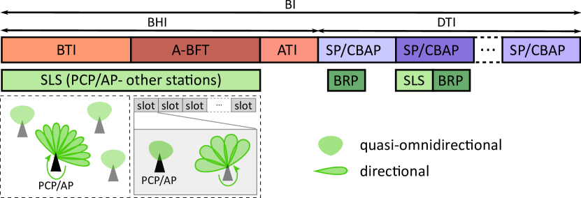
Figure 1: Structure of a BI. Green boxes correspond to beamforming training operations. The BHI is used for SLS with the PCP/AP: during the BTI, the PCP/AP trains its transmitting antenna pattern; during the A-BFT the other stations train their transmitting or receiving antenna patterns in dedicated slots. During the DTI, stations can perform both SLS and BRP phases with the PCP/AP and with other stations [9].

II-A Physical layer

The nominal channel bandwidth in 802.11ad is $2.16$ GHz, and there are up to $4$ channels in the ISM band around $60$ GHz, although channel availability varies from region to region. Only one channel at a time can be used for communication. There are $32$ different MCSs available, grouped into three different PHY layers, namely Control PHY, Single Carrier PHY and OFDM PHY, which differ for robustness, complexity, and achievable data rates. The standard also includes an energy-saving mode for battery-operated devices, which uses the low power Single Carrier PHY.

II-B Beamforming training

802.11ad introduces the concept of antenna sectors, which correspond to a discretization of the antenna space and reduce the number of possible beam directions to try. The standard supports up to four transmitter antenna arrays, four receiver antenna arrays, and 128 sectors per device. Beamforming training is realized in two subsequent stages: the Sector-Level Sweep (SLS) phase and the Beam Refinement Protocol (BRP) phase, that aim at setting up a link between the stations and maximizing the gain, respectively. This mechanism can be performed between two STAs or a STA and the PCP/AP;  the two devices are denoted as initiator and responder depending on who starts the SLS phase. The initiator sequentially tries different transmit antenna sector configurations, while the responder has its received antennas configured in a quasi-omnidirectional pattern and gives a feedback on each sector tried by the initiator, so as to determine the best coarse-grained antenna sector configuration. The SLS phase can be used also to inspect different configuration of the receiving antenna sectors: in this case, the initiator transmits multiple frames on the best known sector and the pairing node switches receiving sector. After a directional link has been established, the BRP phase is used to inspect narrower beams and, possibly, to optimize the antenna weight vectors in case of phased antenna arrays. Since the BRP phase follows the SLS one, a reliable frame exchange is ensured.

II-C Beacon Intervals

Medium access time is divided into Beacon Intervals (BIs), with maximum duration of $1$ s (but typically chosen around $100$ ms [3]). Each BI consists of a Beacon Header Interval (BHI) and a Data Transmission Interval (DTI), as shown in Fig. 1. The BHI replaces the single beacon frame of legacy WiFi networks and is used for synchronization and network management operations and to establish and maintain directional communication links between the STAs and the PCP/AP through beamforming training and beam tracking mechanisms; the DTI is used for data transmission and for beamforming training with the PCP/AP and between STAs.

The BHI includes up to three access periods, all of them optional: the Beacon Transmission Interval (BTI), the Association-Beamforming Training (A-BFT), and the Announcement Transmission Interval (ATI). The BTI is used for SLS beamforming training of the PCP/AP’s antennas and network announcement: the PCP/AP broadcasts beacon frames iterating through different sectors, performing the first part of the SLS phase with the STAs, which have their receiving antennas configured in a quasi-omnidirectional pattern since they do not know a-priori the direction to use to receive the beacons. The SLS phase started in the BTI is completed in the A-BFT, which is divided into slots during which STAs separately train their antenna sectors for communication with the PCP/AP, and provide feedback to the PCP/AP about the sector to use for transmitting to them. Finally, the ATI is used to exchange management information between the PCP/AP and associated and beamtrained stations, such as resource requests and allocation information for the DTI.

II-D Data transmission

The DTI is made up of contention-free SPs for exclusive communication between a dedicated pair of nodes and CBAPs where stations compete for access. SPs and CBAPs can be in any number and combination, and their scheduling is advertised by the PCP/AP through beacons in the BTI and/or specific frames in the ATI. An allocation is defined by several fields, including the type of allocation (SP or CBAP), the addresses of the source and destination STAs involved in the allocation (which can be unicast, multicast or broadcast), its total duration and starting time and the number of blocks it is made of, beamforming training information if needed, and whether the allocation is pseudostatic, meaning that it recurs in subsequent BIs [1]. Note that this schedule is set up prior to the beginning of the DTI. In addition, a dynamic channel time allocation mechanism allows STAs to reserve channel time in almost real-time over both SPs and CBAPs.

Contention-based access. CBAPs follow the Enhanced Distributed Channel Access (EDCA) mechanism, which is an enhanced DCF that includes functionalities to handle traffic categories with different priorities, frame aggregation and block acknowledgments. Stations compete for access and can obtain Transmission Opportunities (TXOPs) (contention-free periods) by winning an instance of EDCA contention or by receiving a Grant frame; the TXOP duration depends on the traffic category.

The DCF is based on Carrier Sense Multiple Access (CSMA) with Collision Avoidance (CSMA/CA): before transmission, the channel needs to be sensed idle for a minimum amount of time, namely a Distributed Interframe Space (DIFS). If the channel is sensed busy, the transmission is postponed: the STA picks a backoff counter uniformly distributed in $\{0,\ldots,W_{i}-1\}$, where $W_{i}$ is the size of the contention window at the $i$-th retransmission attempt. The contention window starts at a minimum value and doubles at each collision, until it saturates to a maximum value. The backoff time counter is decremented as long as the channel is sensed idle, frozen when a transmission is detected on the channel or the CBAP operation is suspended, and reactivated when the channel is sensed idle again for at least a DIFS (after that the CBAP operation has been resumed). When the backoff counter expires, the STA accesses the channel.

In 802.11ad, the channel status is determined through a combined physical and virtual carrier sensing; the former consists in energy or preamble detection over the channel, the latter is realized through Network Allocation Vectors (NAVs). The NAVs are counters based on the transmission duration information announced in Request-To-Send (RTS) and Clear-To-Send (CTS) frames prior to the actual exchange of data and maintain a prediction of future traffic on the medium.

The directional nature of communication at mmWaves makes the carrier sensing operations problematic [3] because there may be possible interference even though the medium was considered to be idle.

Contention-free access. SPs are contention-free periods assigned by the PCP/AP for exclusive communication between a pair of STAs. The directional communication enables the possibility of spatial sharing, i.e., simultaneous SPs involving different STAs can be scheduled, provided that they do not interfere with each other; this requires a preliminary interference assessment phase, which is coordinated by the PCP/AP. Note that building and updating the interference map may result in huge overhead in case of mobility.

Dynamic allocation mechanism. This mechanism is built on scheduled SPs and CBAPs with specific configuration and enables near-real-time reservation of channel time; the dynamic allocations do not persist beyond a BI. Stations can be polled by the PCP/AP and ask for channel time, which will be granted back to back.

The dynamic mechanism also includes the possibility of truncating and extending SPs, to exploit unused channel time and finalize the ongoing communication without additional delay and scheduling, respectively. When an SP is truncated, either the relinquished channel time is used as a CBAP or the PCP/AP polls STAs so that they can ask for channel time.

Resource scheduling. Evidently, there are many elements that need to be taken into account to appropriately schedule the DTI based on the QoS requirements. In addition to modeling data transmission in both CBAP and SP allocations, it is necessary to understand in which cases the dynamic allocation mechanism yields better performance than the predefined schedule. Another aspect that should be taken into consideration is power consumption: the presence of energy constrained devices may require changes in the scheduling, e.g., in the allocation order or by assigning more SP allocations. A critical issue is represented by the beamforming training (see Sec. VI-A) which introduces overhead and may degrade the network performance. Mainly, there are three knobs available to the protocol designer:

• Contention-based or contention free allocation. This is the most meaningful choice as it impacts the way the medium is accessed and thus plays a direct role on the performance. SP allocations grant dedicated resources and the obtained performance only depends on the channel status, being therefore more predictable than when interference comes into play. Clearly, setting up the scheduled sessions introduces overhead and some latency, but the beam steering process is simplified since the receiver knows who is going to transmit and can steer its receiving beam towards the sender, and the STAs not involved in the SP can go to sleep and save power. On the other hand, CBAPs are distributed and robust and good for unpredictable bursty traffic. Nonetheless, carrier sensing may be problematic due to the use of directional antennas. Also, during CBAP period, STAs cannot go into power saving mode due to the inner nature of CSMA/CA. SP allocations are particularly suitable for periodic reporting with QoS demands, but CBAPs may be preferable in case of less stringent QoS requirements because channel resources are available to more stations.

• Pseudo static allocation. In this way, it is possible to decide whether the allocation will recur in successive BIs. This is very useful for predictable traffic patterns as it avoids the need to schedule the allocation every time and limits the signaling overhead.

• Dynamic allocation. It allows quasi-real-time channel use, but has a polling overhead and the scheduled allocation over which it is applied needs to satisfy certain conditions. This feature can be useful for unpredictable transmissions that need to be delivered with specific QoS requirements.

III Related work

The seminal work of [6] introduces a Markov Chain (MC) model of the IEEE 802.11 DCF. Although several variations on such model have been proposed to account for, e.g., finite number of retransmissions [10], heterogeneous QoS [11] and hidden node problem [12], none of them can be readily applied to the hybrid MAC layer of IEEE 802.11ad, as different changes are needed to account for its peculiar features.

Some works in the literature propose adaptations of Bianchi’s model for 802.11ad. Most of them, however, do not model the effect of directional communication properly, as they neglect the deafness and hidden node problems. For example, [13] uses a $3$-dimensional MC model to analyze the channel utilization and the average MAC layer delay that can be obtained in CBAPs. This model accounts for the presence of allocations other than CBAP and for the fact that backoff counters are frozen when CSMA/CA operation is suspended. However, it does not introduce the maximum contention window size, so that the contention window keeps doubling at each retransmission stage. Moreover, the model assumes that CBAPs are allocated to sectors, so that two STAs belonging to different sectors cannot compete for the channel time in the same allocation. According to the standard [1], this is not necessarily true, since any subset of stations can participate in a CBAP, with potential deafness and hidden node issues. The model also erroneously assumes that all STAs in the same sector can overhear the messages that other nodes exchange with the AP. Thus, the assumption made in [13] strongly affects the analysis of the delay and the impact of the number of sectors used by the PCP/AP on the system performance, as the role of directional transmissions and deafness is neglected.

Similar assumptions have been made in [14], which models CBAPs with a $2$-dimensional MC for unsaturated sources considering also the contention-free allocations of 802.11ad. However, besides neglecting the deafness problem, the model assumes that the DTI is made of SP allocations followed by a single CBAP allocation at the end of the DTI, while the standard [1] envisages SP and CBAP allocations in any number and order. This assumption may strongly affect the delay, as different configurations of the DTI may yield different performance. Also [15] uses a $2$-dimensional MC to analyze the saturation throughput in CBAP but neglects the deafness issues and assumes the same specific configuration of the DTI as in [14].

A more accurate approach to directional communication in WiFi networks is presented in [16], which however is not designed for 802.11ad so that it does not consider the presence of SP allocations and the related backoff counter freezing. The model considers an accurate model for directional transmission, with the presence of side lobes with small antenna gain and corresponding regions with different levels of interference. Also [8] takes into account deafness and hidden node problems, and subdivides the area around a STA based on the interference level; CBAPs are then modeled using a $3$-dimensional MC.

Other works in the literature consider different aspects of the DTI. For example, [17] derives the theoretical maximum throughput for CBAPs when two-level MAC frame aggregation is used. [7] proposed a directional MAC protocol to be used on top of 802.11ad: it allows the use of sequential directional RTS messages that a STA sends in all directions and that can therefore be overheard by all other STAs. The beamforming issue is considered in [18], which proposes a joint optimization of beamwidth selection and scheduling to maximize the effective network throughput.

For what concerns SPs, an accurate mathematical model for their preliminary allocation is presented in [19]. It considers the presence of quasi-periodic structures with multiple blocks within the same allocation, the erroneous nature of the wireless medium, and the possibility of multiple consecutive transmissions within the same allocation. A $3$-dimensional MC is used to model a Variable Bit Rate (VBR) flow with packets arriving in batches of random size at regular intervals and can be used to derive the optimal SP allocation that satisfies the QoS requirement.

IV System model

We now introduce our analytical model for CBAP operation in 802.11ad. We denote as $T_{\rm BI}$ the duration of a BI and as $T_{\rm BHI},T_{\rm CBAP}$ and $T_{\rm SP}$ the time dedicated to BHI, CBAPs and SPs during a BI, respectively. The total time $T_{\rm CBAP}$ dedicated for contention-based access in a BI is distributed among $N_{\rm CBAP}$ allocations with the same duration, while $T_{\rm SP}$ is distributed among $N_{\rm SP}$ allocations with the same duration.

We make two assumptions: i) all STAs in the network implement a single Access Category (AC) only, hence service differentiation is not considered, and ii) the beamforming training has already been performed, so that the STAs already know how to steer their antennas to communicate with the AP. Also, we only focus on the classic WiFi network where a certain number of STAs communicate solely with the AP; we consider that the RTS/CTS mechanism is used.

To assess the performance that can be obtained in a CBAP, we leverage on Bianchi’s seminal work [6] and adapt it to model the features of CBAPs in 802.11ad. First of all we explain how directionality affects the communication during the contention-based channel access, then we describe the proposed model, and finally we discuss the performance metrics used in the numerical evaluation.

IV-A Directional communication in CBAPs

Besides the need of beamforming training and beam tracking mechanisms, the directional nature of communication in 802.11ad implies substantial changes also from a data transmission perspective. As explained in Sec II-D, CBAPs are based on the EDCA; however, the traditional approaches used in the literature need to be adapted to take directionality into account, since the consequent deafness and hidden node problems may significantly affect the system performance.

The most widely used approach in the literature to model the DCF and EDCA mechanisms is Bianchi’s model [6]. It takes the perspective of a target node and models the backoff process as a two dimensional MC, where state $(i,k)$ refers to the $i^{\rm th}$ backoff stage with the backoff counter $k\in\{0,\ldots,W_{i}-1\}$, where $W_{i}$ is the duration of the contention window at the $i^{\rm th}$ retransmission attempt. The counter is decremented with probability $1$ whenever the channel is sensed idle; when it reaches $0$, the STA attempts to transmit. The time spent in each state depends on what happens in the channel meanwhile, as it may be idle, used for a successful transmission, or used simultaneously by colliding STAs. The original model was proposed for omnidirectional communication, so that each STA is aware of ongoing transmissions and can defer its own when it senses the channel to be idle. Collisions only happen when multiple STAs access the channel simultaneously because their backoff counters expired (at least two STAs are in a state $(\cdot,0)$).

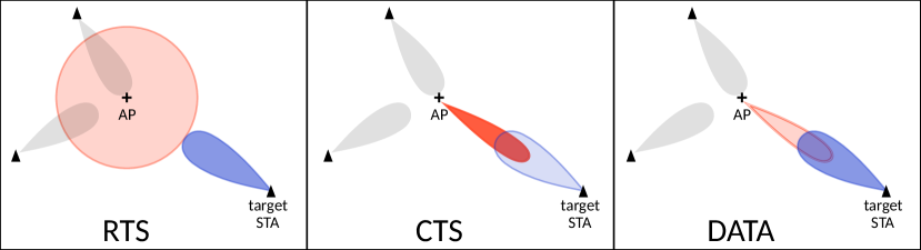
Figure 2: Communication phases between the AP and a target STA and two other STAs that listen in direction of the AP. Darker beams indicate a transmission, while lighter ones indicate that the device is listening. The target STA directionally transmits the RTS while the AP is listening in QO mode; then the AP steers its transmitting antennas towards the target STA and sends the CTS to the target STA, which then replies transmitting a data message.

In the case of directional communication, however, STAs may not hear ongoing transmissions, resulting in a much higher collision probability. In this work, we assume that the RTS/CTS mechanism is used. Since a STA communicates only with the AP, it always has both its transmitting and receiving antenna patterns configured towards it. The AP instead listens to the channel in a quasi-omnidirectional (QO) mode, and, upon the reception of an RTS, it switches its antenna configuration to point towards the STA that sent it. Fig. 2 illustrates the direction of the various phases of the communication between a STA and the AP. Note that the messages can be heard only by a limited number of other STAs. The received power $P_{\rm rx}$ at a STA is in fact

$$P_{\rm rx}=P_{\rm tx}\frac{g_{\rm tx}(\theta_{\rm tx},\varphi_{\rm rx})g_{\rm rx}(\theta_{\rm tx},\varphi_{\rm rx})}{Ad^{\eta}}$$ (1)

where $P_{\rm tx}$ is the power used to transmit, $d$ is the distance from the transmitter, $\eta$ is the path-loss exponent, $A$ is a normalizing path-loss term, and $g_{\rm tx}$ and $g_{\rm rx}$ are the antenna gains of the transmitter and receiver, respectively. They both depend on the direction of the antennas with respect to the line of sight between the two STAs, thus on the angles $\theta_{\rm tx}$ and $\varphi_{\rm rx}$. If the gains are very small, $P_{\rm rx}$ may be too low in order for the receiver to decode the signal properly.

Consider a network consisting of $n$ STAs and a target STA that communicates with the AP, so that the STA and the AP point to each other, and the antenna gains in the other directions are minimal. It is possible to cluster the other $n-1$ STAs into four groups:

• $n_{I,1}$: STAs that can overhear the messages sent from the target STA to the AP but not those sent from the AP to the STA.

• $n_{I,2}$: STAs that can overhear the messages from the AP to the target STA but not those from the STA to the AP.

• $n_{I,3}$: STAs that can overhear the whole communication between the AP and the target STA.

• $n_{I,4}$: STAs that cannot overhear any messages exchanged between the AP and the target STA.

Analogously, from the perspective of a STA that listens to the channel, the other STAs can be divided into four groups $n_{O,1}$ (STAs of which it can hear the messages to the AP but not the messages that the AP sends to them), $n_{O,2}$ (STAs of which it cannot hear the messages to the AP but can hear those that the AP sends to them), $n_{O,3}$ (STAs of which it can hear all the messages exchanged with the AP), and $n_{O,4}$ (STAs whose messages exchanged with the AP cannot be heard).

Consequently, collisions can happen at three different stages of the uplink communication from a target STA to the AP.

1. The target STA accesses the channel to transmit its RTS, but collides for sure. This can happen for three different reasons: i) if any other STA accesses the channel at the same time, as in the legacy WiFi, ii) if a STA belonging to groups $n_{O,2}$ or $n_{O,4}$ is transmitting the RTS to the AP, or iii) if a STA in group $n_{O,4}$ has already sent the RTS and is going on with the communication with the AP. Notice that, in the latter case, the transmission of the target STA fails, because the AP is listening in the direction of the STA from group $n_{O,4}$, but the ongoing data transmission may still be successful, as the directionality highly attenuates the interference. In this work we assume that, except for errors in the channel, the ongoing data transmission is successful.

2. If none of the previous conditions happened, the transmission of the RTS may still be vulnerable to interference. This happens when a STA in groups $n_{I,2}$ or $n_{I,4}$ accesses the channel meanwhile. The packets will then collide.

3. If the transmission of the RTS was successful, the AP sends the CTS and the target STA can proceed with the data transmission. However, a STA in group $n_{I,4}$ is unaware of the ongoing communication and may try to access the channel. As assumed in case 1iii), the outcome of the ongoing transmission only depends on channel errors, while the STA that accesses the channel will register a collision.

In the remainder of this section, we propose an adaptation of Bianchi’s model that accounts for the directionality of transmissions, assuming that the regions corresponding to the four groups of nodes are known; Sec. VI introduces an analytical model to compute such regions when constant-gain beam shapes are used.

$$b_{0,0} =\begin{dcases}\frac{2(1-2p)(1-p)}{W_{0}(1-(2p)^{m+1}(1-p)+(1-p^{m+1})(1-2p)}\qquad\qquad\qquad\qquad\qquad\qquad\qquad\;\;\>\text{if }m\leq m^{\prime}\\ \\ \frac{2(1-2p)(1-p)}{W_{0}(1-(2p)^{m^{\prime}+1})(1-p)+2^{m^{\prime}}W_{0}(p^{m^{\prime}}-p^{m})(1-2p)p+(1-p^{m+1})(1-2p)}\qquad\text{if }m>m^{\prime}\end{dcases}$$ (4)

 

IV-B Rethinking Bianchi’s model

Bianchi’s model [6] needs three major adaptations in order to be suitable for 802.11ad, which are caused by the following features.

1. CBAPs can be interrupted because there is a scheduled SP or the BHI of the next BI. In this case, all backoff counters have to freeze [1]; they will be restored in the next CBAP. This affects the time that a STA spends in a state $(i,k),\,k\in\{1,\ldots,W_{i}-1\}$ before decrementing its backoff counter and transitioning to $(i,k-1)$; the transition probability from $(i,k)$ to $(i,k-1)$ is $1$ as in Bianchi’s original model. We denote the freezing probability as $p_{f}$.

2. The finite duration of CBAPs may also cause transmissions deferral. In fact, if the backoff counter of a STA reaches $0$ but there is not enough time to complete a transmission, that STA should refrain from transmitting. The standard [1] however does not specify how to handle the backoff counter in this case. A possibile strategy consists in freezing it when it expires and then restoring it in the next CBAP, as in case 1, so that the involved STA can transmit as soon as the EDCA operation starts again. However, such approach may easily lead to collisions: if the counters of multiple STAs expire during the time needed for a complete transmission at the end of the current CBAP, and they all get frozen to $0$, all such STAs will attempt accessing the channel simultaneously in the next CBAP. To avoid this, we propose to use the same approach used in [14], so that a new backoff counter is randomly chosen from the current window (no collision happened). This causes the addition of new transitions from state $(i,0)$ to $(i,k),\,k\in\{0,\ldots,W_{i}-1\}$. We denote the probability of insufficient time in the current CBAP as timeout probability $p_{t}$.

3. As discussed in Sec. IV-A, the directional nature of mmWave communication has a huge impact on the operation of the DCF mode because of deafness and the increased hidden node problem. This modifies the collision probability and the time spent in each state, which depend on the behavior of STAs whose transmissions can be detected by the target STA.

Fig. LABEL:fig:macro_mc represents the MC we propose to model the behavior of a STA during CBAP operation. As in Bianchi’s model, a state $(i,k),\,i\in\{0,\ldots m\},\,k\in\{0,\ldots,W_{i}-1\}$ refers to the $i^{\rm th}$ backoff stage with the backoff counter being equal to $k$. Here, $m$ is the maximum number of retransmissions. The contention window in stage $i$ is $W_{i}=\min\{2^{i}W_{0},2^{m^{\prime}}W_{0}\}$, where the initial window $W_{0}$ and the maximum window $2^{m^{\prime}}W_{0}$ are defined in the standard.

From a state $(i,k),\,k\!>\!0$, the backoff counter is decremented with probability $1$ (solid black transitions in Fig. LABEL:fig:macro_mc), but the time needed to transition to the next state $(i,k\!-\!1)$ is variable, depending on how the channel is being used. When it reaches a state $(i,0)$, the STA might be constrained to defer its transmission (adaptation 2). The residual time in the current CBAP is uniformly distributed in $[0,T_{\rm CBAP}/N_{\rm CBAP}]$, where $T_{\rm CBAP}/N_{\rm CBAP}$ is the average duration of a CBAP allocation in the BI. Then, the probability that there is no sufficient time to complete a transmission of duration $T_{L}$ can be approximated as

$$p_{t}=\frac{T_{L}}{T_{\rm CBAP}/N_{\rm CBAP}}\,.$$ (2)

Thus, from each state $(i,0),i\in\{0,\ldots m\}$, the MC transitions to a state $(i,k),\,k\in\{0,\ldots,W_{i}-1\}$ with probability $p_{t}/W_{i}$ (dotted orange transitions in Fig. LABEL:fig:macro_mc), while with probability $1-p_{t}$ the STA accesses the channel. We identify such latter condition as being in a transmission state (the MC is in a state $(i,0)$ and attempts to transmit); when the other condition applies (transmission deferral) or the MC is in a state $(i,k),\,k>0$, we say that the STA is in a non-transmission state. As in [7], each transmission state is itself a MC, which will be described in Sec. IV-C; thus, in order not to generate confusion, we will refer to the MC of Fig. LABEL:fig:macro_mc as macro MC.

Let $p$ be the failure probability, which includes the collision probability (see the discussion in Sec. IV-A) and the error probability due to the wireless channel, as explained later. Then, from state $(k,0)$ the MC goes to a state $(0,i),i\in\{0,\ldots,W_{0}-1\}$ (successful transmission of a new packet; solid green transitions in Fig. LABEL:fig:macro_mc) with probability $(1-p_{t})(1-p)/W_{0}$, or to any state $(k+1,i),i\in\{0,\ldots,W_{k+1}-1\}$ with probability $(1-p_{t})p/W_{k+1}$ (dashed red transitions in Fig. LABEL:fig:macro_mc). If it reaches the maximum number of retransmission attempts ($k=m$), the MC goes from state $(m,0)$ to a state $(0,i),\,i\in\{0,\ldots,W_{0}\}$ with probability $(1-p_{t})/W_{0}$.

It is then possible to compute the steady-state probabilities $\{b_{i,k}:i\!\in\!\{0,\ldots,m\},k\!\in\!\{0,\ldots W_{i}-1\}\}$ of the macro MC, using the same approach of [6]. Assuming $p_{t}<1$, it is

$$b_{i,k}=\frac{W_{i}-k}{W_{i}}p\,b_{0,0}\,,$$ (3)

where $b_{0,0}$ is given in (4). Notice that $b_{0,0}$ does not depend on $p_{t}$, which, nonetheless, has an impact on the delay.

The probability of being in a transmission state is then

$$\tau=\sum_{i=0}^{m}b_{i,0}(1-p_{t})=\frac{1-p^{m+1}}{1-p}(1-p_{t})b_{0,0}\,.$$ (5)

The time spent, on average, in a transmission or non transmission state is denoted as $\mathrm{E}\left[T_{\rm tx}\right]$ and $\mathrm{E}\left[T_{\rm ntx}\right]$, respectively, which depend on the probabilities $\{b_{i,k}\}$ as explained next. It is then possible to define the probability $\pi_{\rm tx}$ that, in an arbitrary time instant, the macro MC is in a transmission state:

$$\pi_{\rm tx}=\frac{\tau\mathrm{E}\left[T_{\rm tx}\right]}{\tau\mathrm{E}\left[T_{\rm tx}\right]+(1-\tau)\mathrm{E}\left[T_{\rm ntx}\right]}\,.$$ (6)

With probability $1-\pi_{\rm tx}$, in an arbitrary time instant, the MC will be in a non transmission state. Note that (6) refers to the semi-Markov model, while (5) refers to the corresponding embedded MC.

To derive $\mathrm{E}\left[T_{\rm tx}\right]$ and $\mathrm{E}\left[T_{\rm ntx}\right]$ it is first necessary to understand what happens in a transmission state.

IV-C A transmission state

Whenever a STA is in a transmission state $(i,0),\,i\in\{0,\ldots m\}$, it attempts to transmit with probability $1-p_{t}$, while with probability $p_{t}$ it picks a new backoff counter from the same window $W_{i}$ (see (2)) and enters a transmission state.

To model such a behavior, each transmission state forms its own MC, similarly to the model proposed in [7]. The MC is made of $6$ states: the access state $A$, the collision RTS state $R_{c}$, the vulnerable RTS state $R_{v}$, the ongoing transmission state $O$, the failure state $F$, and the success state $S$. A STA goes into state $A$ when it accesses the channel and goes from the macro MC into the transmission state MC. It transmits the RTS to the AP, and, based on the discussion in Sec. IV-A, two cases can occur.

• As soon as the STA accesses the channel, it may immediately collide (case 1 in Sec. IV-A). This happens with probability $p_{c,1}$; in this case, the STA transitions to state $R_{c}$ where it transmits the RTS and then, with probability 1, goes to the failure state $F$.

• Otherwise, the transmission of the RTS is still vulnerable to interference. If it collides (case 2 of Sec. IV-A), the MC transitions to the failure state $F$; this happens with probability $p_{c,2}$. Otherwise, the STA goes to state $O$, where it receives the CTS from the AP and then sends its data. In turn, the data transmission may fail because of channel errors (but not because of interference, as assumed in Sec. IV-A) and therefore, with probability $p_{e}$, the next state in the MC is $F$. Otherwise, the transmission is successful and the next state in the MC is $S$. Then, from either $F$ or $S$, the STA exits the transmission state.

The resulting MC is represented in Fig. 4. Let $b_{j}$ be the steady-state probability that the MC is in state $j\in\mathcal{J}_{\rm tx}\triangleq\{A,R_{c},R_{v},O,F,S\}$. The transmission state itself forms a MC where the outgoing transitions from states $S$ and $F$ re-enter the transmission state from state $A$. Thus, the steady-state probabilities are: $b_{A}=1/b_{\rm tx},\,b_{R_{c}}=(1-p_{c,1})/b_{\rm tx},\,b_{R_{v}}=p_{c,1}/b_{\rm tx},\,b_{O}=(1-p_{c,1})(1-p_{c,2})/b_{\rm tx},\,b_{F}=(1-(1-p_{c,1})(1-p_{c,2})(1-p_{e}))/b_{\rm tx},b_{S}=(1-p_{e})(1-p_{c,1})(1-p_{c,2})/b_{\rm tx}$, where $b_{\rm tx}=3+p_{e}(1-p_{c,1})(1-p_{c,2})$.

Similarly to what done for the macro MC, it is possible to define the probabilities $\pi_{j}$ that, in an arbitrary time instant, given that the MC is in a transmission state, the MC is in state $j\in\mathcal{J}_{\rm tx}$:

$$\pi_{j}=\frac{T_{j}b_{j}}{\sum_{\ell\in\mathcal{J}_{\rm tx}}T_{\ell}b_{\ell}}\quad j\in\mathcal{J}_{\rm tx}\,,$$ (7)

where $T_{j}$ is the time spent in state $j$. Through $b_{j}$, the probabilities $\pi_{j},j\in\mathcal{J}_{\rm tx}$ depend on the collision and error probabilities $p_{c,1}$, $p_{c2,}$ and $p_{e}$. The collision probabilities in turn depend on how many and which other STAs access the channel while the target STA is in the transmission state, and thus on $\pi_{j}$.

Considering the model in Sec. IV-A where STAs can be grouped based on what they can hear of a communication between the AP and another STA, $p_{c,1}$ is given by the probability that none of these three cases occurs: i) any of the other STAs accesses the channel simultaneously, ii) at least a STA in group $n_{O,2}$ is transmitting an RTS to the AP, or iii) at least a STA in group $n_{O,4}$ is using the channel. We analyze the probabilities of these events.

Case i) occurs if at least another STA is accessing the channel, given that the target STA is accessing the channel. The probability of this to happen can be expressed as:

$$q_{1} =\frac{1-(1-p_{\rm acc})^{n}-np_{\rm acc}(1-p_{\rm acc})^{n-1}}{p_{\rm acc}}\,,$$ (8)

where $n$ is the total number of STAs in the network and $p_{\rm acc}=\pi_{A}\pi_{\rm tx}$ is the probability that a STA is accessing the channel.

Figure 4: Markov chain that models a transmission state. It is entered from i) state $(i,1)$ with probability $1-p_{t}$, ii) state $(i-1,0$) with probability $p(1-p_{t})/W_{0}$ or iii) state $(i,0)$ itself with probability $p_{t}/W_{0}$.

Case ii) happens if at least a STA in group $n_{O,2}$ is either in state $R_{v}$ or in $R_{c}$, given that the target STA is accessing the channel. Thanks to Bayes’ rule, the probability of this to occur can be equivalently expressed as a function of the probability that the target STA accesses the channel given that at least a STA in group $n_{O,2}$ is either in state $R_{v}$ or in $R_{c}$. This is not trivial to compute, because it requires an analytical expression for the relations between the coverage areas of multiple STAs. In fact, if a STA in group $n_{O,2}$ entered a transmission state, all STAs that can hear it refrain from transmitting, so that the number of STAs that compete for the channel is reduced and it is more likely that the target STA senses the channel as idle and attempts transmitting. However, we do not consider such relations, which are extremely challenging to model, but only account for the fact that, if some STAs are in a transmission state, the ECDA operation is not frozen, so that the access probability is increased by a factor $1/(T_{\rm CBAP}/T_{\rm BI})$. We thus express the probability of case ii) as

$$q_{2}=\frac{1-(1-\pi_{\rm tx}(\pi_{R_{v}}+\pi_{R_{c}}))^{n_{O,2}}}{T_{\rm CBAP}/T_{\rm BI}}\,.$$ (9)

As the numerical evaluation of Sec. VII shows, this approximation affects the validity of the model only for highly dense scenarios, with more than $100$ STAs.

Finally, case iii) can be treated analogously to case ii) and thus happens with probability

$$q_{3}=\frac{1-(1-\pi_{\rm tx}(\pi_{R_{v}}+\pi_{R_{c}}+\pi_{O}))^{n_{O,4}}}{T_{\rm CBAP}/T_{\rm BI}}\,.$$ (10)

Then, the probability of colliding while accessing the channel is

$$p_{c,1}=1-(1-q_{1})(1-q_{2})(1-q_{3})\,.$$ (11)

since there is a collision if at least one of cases i), ii), iii) occurs.

When the target STA did not collide while attempting to transmit and is thus in state $R_{v}$, it collides if at least a STA that cannot hear the uplink messages sent by the target STA accesses the channel during the whole duration of $R_{v}$. Following the same reasoning as per (9) and (10), this happens with probability

$$p_{c,2}=\frac{1-((1-p_{\rm acc})^{n_{I,2}+n_{I,4}})^{T_{R_{v}}/T_{A}}}{T_{\rm CBAP}/T_{\rm BI}}\,.$$ (12)

Eqs. (7), (11), (12) form a nonlinear system in the unknowns $\pi_{j},p_{c,1}$ and $p_{c,2}$, which can be solved using numerical techniques, as in Bianchi’s original model. The error probability $p_{e}$ instead depends on the Signal-to-Noise-Ratio (SNR) and the MCS used.

V Performance metrics

We evaluate the performance achievable in a CBAP in terms of throughput, delay and dropping rate. Before delving into their description, it is useful to derive the time spent in a transmission and non transmission state.

V-A Average time spent in a transmission state

A STA that accesses a transmission state can follow $4$ different paths, depending on collision and errors. The average time spent in a transmission state is thus the sum of the time associated to each of these paths, weighed for the probability of that path:

$$\mathrm{E}\left[T_{\rm tx}\right] =(T_{A}+T_{R_{c}}+T_{F})p_{c,1}$$ (13)

$$+(T_{A}+T_{R_{v}}+T_{F})(1-p_{c,1})p_{c,2}$$

$$+(T_{A}+T_{R_{v}}+T_{O}+T_{F})(1-p_{c,1})(1-p_{c,2})p_{e}$$

$$+(T_{A}+T_{R_{v}}+T_{O}+T_{S})(1-p_{c,1})(1-p_{c,2})(1-p_{e}).$$

This can be easily seen in Fig. 4.

The probabilities $\pi_{j}$ are defined in (7) and the times $T_{j}$ are as follows: $T_{A}=\delta,\,T_{R_{c}}=RTS,\,T_{R_{v}}=RTS,\,T_{O}=CTS+\mathrm{E}\left[T_{L}\right]+ACK+3SIFS+3\delta,T_{F}=DIFS,T_{S}=DIFS$, where $\delta$ is the propagation delay, $RTS$ and $CTS$ represent the time needed to send an RTS and CTS message, respectively, $\mathrm{E}\left[T_{L}\right]$ is the average time needed to transmit a data packet, $ACK$ is the time to send an ACK, and $SIFS$ and $DIFS$ represent the Short Interframe Space (SIFS) and DIFS durations, respectively [1].

V-B Average time spent in a non-transmission state

The time spent in a non-transmission state depends on what happens meanwhile: the CBAP may freeze, the target STA may hear a transmission or sense the channel as idle. The EDCA mechanism assumes that the backoff counter is decremented only after the channel is sensed idle for a time slot of duration $\sigma$ (which is defined in the standard and depends on the PHY layer). Before that, the CBAP may freeze or be busy. We can interpret the freezing condition as a self-loop on a state $(i,k),\,k>0$ with probability

$$p_{f}=1-\frac{T_{\rm CBAP}}{T_{\rm BI}}\,,$$ (14)

so that on average $1/(1-p_{f})$ iterations over $(i,k)$ are expected before a transition to $(i,k-1)$.

The target STA senses the channel as idle when none of the STAs in groups $n_{I,1}$ and $n_{I,3}$ is using the channel (i.e., is in any of the states $A,R_{c},R_{v},O$) and none of the STAs is using the channel and has already received a feedback from the AP (i.e., it is in state $O$):

$$p_{i}=(1-\pi_{\rm tx}(\pi_{A}+\pi_{R_{c}}+\pi_{R_{v}}+\pi_{O}))^{n_{I,1}+n_{I,3}}(1-\pi_{\rm tx}\pi_{O})^{n_{I,2}}\,,$$ (15)

The channel is sensed as busy with probability $1-p_{i}$ for an average duration of $E_{\rm tx}$. Thus, the average time spent in a non-transmission state can be expressed as

$$\mathrm{E}\left[T_{\rm ntx}\right]=\sigma+\frac{(1-p_{i})E_{\rm tx}}{1-p_{f}}\,.$$ (16)

V-C Throughput

The normalized system throughput $S$ is defined as the fraction of time that the channel is used to successfully transmit information. The average payload size is $\mathrm{E}\left[L\right]$ and a transmission is successful with probability $\pi_{\rm tx}(1-p)$. Thus the aggregated throughput is

$$S=n\frac{\pi_{\rm tx}(1-p)\mathrm{E}\left[L\right]}{\pi_{\rm tx}\mathrm{E}\left[T_{\rm tx}\right]+(1-\pi_{\rm tx})\mathrm{E}\left[T_{\rm ntx}\right]}$$ (17)

where the denominator represents the average duration of a time slot and $n$ is the number of STAs in the network.

V-D Delay

The delay experienced by a (successfully transmitted) packet is the time elapsed from when it arrived at the MAC layer until it is received. Let $\mathrm{E}\left[D_{i}\right]$ denote the expected delay that a packet experiences when it is successfully transmitted at stage $i$, $\mathrm{TX(i)}$ the event of transmission at stage $i$, and $\mathrm{success}$ the event of a successful transmission. Then

$$\mathrm{E}\left[D\right]=\sum_{i=0}^{m}{\rm Pr}(\mathrm{TX}(i)|\mathrm{success})\mathrm{E}\left[D_{i}\right]$$ (18)

where ${\rm Pr}(\mathrm{TX}(i)|\mathrm{success})$ represents the probability that, given that a successful transmission happened, it was at stage $i$. The event $\mathrm{success}$ happens when the packet is not discarded after $m$ backoff stages, i.e., with probability $1-p^{m+1}$, since a packet is dropped if its transmission fails (with probability $p$) at stages $0,1,\dots,m$. Thus ${\rm Pr}(\mathrm{TX}(i)|\mathrm{success})=(1-p)p^{i}/(1-p^{m+1})$ since the packet was discarded at stages $0,1,\ldots,i-1$ and then successfully transmitted at stage $i$. The term $\mathrm{E}\left[D_{i}\right]$ is the sum of the average backoff process delay in stages $0,1,\ldots,i$, the collision delay experienced in stages $0,1,\ldots,i-1$, and the time needed for the successful transmission at stage $i$. The first state $k$ in the $j^{{\rm th}}$ backoff stage is uniformly distributed between $0$ and $W_{j}-1$; the counter is decremented until state $(j,0)$ ($k+1$ states are crossed) and then, with probability $p_{t}$ there is a transition back to a random state at stage $j$. Therefore, the delay term is:

$$\mathrm{E}\left[D_{i}\right]=iT_{c}+T_{s}+\mathrm{E}\left[T_{\rm ntx}\right]\sum_{j=0}^{i}\sum_{\ell=0}^{+\infty}p_{t}^{\ell}\sum_{k=0}^{W_{j}-1}\frac{k+1}{W_{j}}$$ (19)

$$=iT_{c}+T_{s}+\frac{\mathrm{E}\left[T_{\rm ntx}\right]}{1-p_{t}}\sum_{j=0}^{i}\frac{W_{j}+1}{2}$$

$$=iT_{c}+T_{s}+\frac{\mathrm{E}\left[T_{\rm ntx}\right]}{2(1-p_{t})}(2^{\min(i,m^{\prime})+1}\!-\!1\!+\!\max(i\!-\!m^{\prime},0)2^{m^{\prime}})W_{0}$$

where $\mathrm{E}\left[T_{\rm ntx}\right]$ is the time spent in a backoff state and $T_{c}$ and $T_{s}$ are the durations of a successful transmission and a collision, respectively:

$$T_{s} =RTS+CTS+\mathrm{E}\left[T_{L}\right]+ACK+3SIFS+4\delta\,,$$ (20)

$$T_{c} =RTS+DIFS+\delta\,.$$ (21)

VI A model for directional communication

The model of Sec. IV-A assumes to know the number of STAs that can overhear the uplink and downlink messages exchanged between the AP and a target STA, which is equivalent to characterizing the regions around the target STA corresponding to groups $n_{I,1}$, $n_{I,2}$, $n_{I,3}$ and $n_{I,4}$. This is not trivial to compute as the power received at a STA depends on the gains of the transmitting and receiving antennas, as per (1), which vary according to the considered direction (angles $\theta_{\rm tx}$ and $\varphi_{\rm rx}$ in (1)). In the following, we describe the model we use for the beam shapes and then provide a mathematical approach to compute the areas corresponding to each group of STAs.

VI-A Beam shapes

The directivity of an antenna depends on the shape of a beam. There exists a multitude of models for antenna beams, such as the Gaussian beam shape, the sinc beam shape and the sampled beam shape, which, however, are very challenging to be used in mathematical models. A simpler approach is given by the constant-gain beam shape (sometimes called pizza-slice beam shape), where the space around the device is divided into $N_{b}$ beams with constant beamwidth $W_{b}=2\pi/N_{b}$; a beam has constant gain in the main lobe and there are no side lobes. From the expression of the directivity of an antenna [20], the antenna gain for a beam centered at $\varphi$ is $g(\theta)=N_{b}$ if $\theta\in\left[\varphi-\frac{W_{b}}{2},\varphi+\frac{W_{b}}{2}\right]$, and $0$ otherwise.

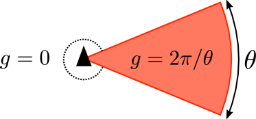
Figure 5: Pizza-slice beam of width $\theta$. The antenna gain is $2\pi/\theta$ within the beam, $0$ outside.

We assume homogeneous STAs with the same antenna gains; however it makes sense to consider the AP to be more powerful than the STAs and with narrower beams. Thus, we denote as $N_{\rm AP}$ and $N_{\rm S}$ the number of sectors for the AP and a STA, respectively. We assume that $N_{\rm AP}\geq 2$ and $N_{\rm S}\geq 2$.

As explained in Sec. IV-A, since the STAs only communicate with the AP, they always have their transmitting and receiving antennas directed towards it. The AP instead listens in a QO mode and switches to directional mode when engaged in a communication with a STA. In this work, we assume that the QO mode coincides with omnidirectionality and yields a unitary gain, and leave to future work the investigation of smaller widths.

We also assume full transmitter/receiver reciprocity, meaning that a STA uses the same sector to transmit to and receive from the AP, and vice versa. The antenna gains of the AP and STA in directional mode computed with the model in Sec. VI-A are $g_{\rm AP}\equiv N_{\rm AP}$ and $g_{\rm S}\equiv N_{\rm S}$ in the main lobes, respectively, and zero outside (see Fig. 5).

As a final remark, we highlight that, as in most of the literature, we consider only 2D directivity, which highly simplifies the problem, although antennas clearly have a 3D radiation pattern.

VI-B Coverage area and power regulations

Since there are no side lobes, two STAs can hear each other only if they are in each other’s main lobe, respectively. Given this and considering the average, it is possible to derive a maximum transmission range by means of a threshold $\gamma_{\rm th}$ on the SNR $\gamma=P_{\rm rx}/N$, where $N$ is the noise power. Then, using (1), the distance $d$ between two devices should be

$$d\leq\left(\frac{P_{\rm tx}g_{\rm tx}(\theta_{\rm tx},\varphi_{\rm rx})g_{\rm rx}(\theta_{\rm tx},\varphi_{\rm rx})}{\gamma_{\rm th}AN}\right)^{1/\eta}\,.$$ (22)

The threshold $\gamma_{\rm th}$ can be computed by imposing a maximum tolerable Bit Error Rate (BER) and deriving the corresponding SNR (note that this depends on the MCS used). The antenna gains of the AP and STA are computed as described in Sec. VI-A.

Interestingly, if the AP and the STA have different transmission powers, there is an SNR asymmetry between downlink and uplink when considering the same noise level at receiver and transmitter (see (1) and (22)). We assume the coverage radius $R$ to be bounded by the most stringent limit (22) between uplink ($P_{\rm tx}$ and $g_{\rm tx}$ are those of the STA, $g_{\rm rx}$ is that of the AP which can be listening in either QO or directional mode) and downlink communication ($P_{\rm tx}$ and $g_{\rm tx}$ are those of the AP, $g_{\rm rx}$ is that of the STA). Then, we consider an area ${\mathcal{R}}=\pi R^{2}$ around the AP and the STAs uniformly distributed according to a Poisson Point Process of intensity $\lambda$.

VI-C Stations that overhear uplink messages

We consider a Cartesian plane whose origin coincides with the center of area ${\mathcal{R}}$, so that the AP is in $(0,0)$. Without loss of generality, we assume that the target STA is in $(d_{t},0),d_{t}\in[0,R]$. Considering the beam model of Sec. VI-A, the interferer can overhear uplink communication from the target STA to the AP if it is in the main lobe of the target STA and vice versa, otherwise the received power is $0$ as per (1). Consider an interferer STA at distance $d_{i}\in[0,R]$ from the AP. It can overhear the uplink communication if and only if the phase of its polar coordinates is in the range $[\varphi_{\rm lim}(d_{i}),2\pi-\varphi_{\rm lim}(d_{i})]$, where

$$\varphi_{\rm lim}(d_{i})=\begin{cases}&\pi-\dfrac{\theta_{\rm S}}{2}-\arcsin\left(\dfrac{d_{i}}{d_{t}}\sin\left(\dfrac{\theta_{{\rm S}}}{2}\right)\right)\;\text{if}\;d_{i}\leq d_{t}\\ &\pi-\dfrac{\theta_{\rm S}}{2}-\arcsin\left(\dfrac{d_{t}}{d_{i}}\sin\left(\dfrac{\theta_{{\rm S}}}{2}\right)\right)\;\text{if}\;d_{i}>d_{t}\end{cases}$$ (23)

The proof of this result is provided in Appendix A.

Considering all possible distances $d_{i}$, we obtain the expected area of STAs that can overhear uplink messages given the position of the target node $(d_{t},0)$ as

$${\mathcal{R}}_{R}(d_{t}) =\int_{0}^{R}\int_{\varphi_{\rm lim}(d_{i})}^{2\pi-\varphi_{\rm lim}(d_{i})}r\partial\theta r\,\partial r=\pi R^{2}-2\int_{0}^{R}\varphi_{\rm lim}(r)r\,\partial r$$ (24)

$$=\pi R^{2}-2\int_{0}^{d_{t}}\left(\pi-\frac{\theta_{\rm S}}{2}-\arcsin\left(\frac{r}{d_{t}}\sin\frac{\theta_{{\rm S}}}{2}\right)\right)r\,\partial r$$

$$-2\int_{d_{t}}^{R}\left(\pi-\frac{\theta_{\rm S}}{2}-\arcsin\left(\frac{d_{t}}{r}\sin\frac{\theta_{{\rm S}}}{2}\right)\right)r\,\partial r$$

which can be solved in closed form.

The expected area of STAs that can overhear uplink messages is obtained by averaging (24) over $d_{t}$:

$$\mathrm{E}\left[{\mathcal{R}}_{R}\right] =\int_{0}^{R}{\mathcal{R}}_{R}(d_{t})\frac{2d_{t}}{R^{2}}\partial d_{t}$$ (25)

which also can be solved in closed form and only depends on the beam width $\theta_{\rm S}$.

Rigorously, the power received at STAs that are too far from the target STA is too small so that they should be excluded from ${\mathcal{R}}_{R}$; however, as usually done in the literature, we neglect this issue and leave it for future investigation.

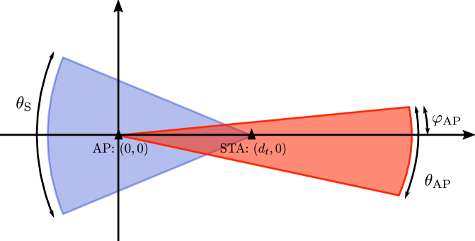
Figure 6: Location of the AP and the target STA in the Cartesian plane. The red beam is the AP beam in the direction of the STA, has width $\theta_{\rm AP}$ and goes from $\varphi_{\rm AP}-\theta_{\rm AP}$ to $\varphi_{\rm AP}$; the blue beam is the STA beam in the direction of the AP and has width $\theta_{\rm S}$.

VI-D Stations that overhear downlink messages

Without loss of generality we keep assuming that the target STA is in $(d_{t},0)$, and consider it to be in a random angular position within the AP sector that covers it, which has width $\theta_{\rm AP}$. We thus denote as $\varphi_{\rm AP}\in[0,\theta_{\rm AP}]$ the angular phase of such sector, so that it spans the angles in the Cartesian plane in the range $[\varphi_{\rm AP}-\theta_{\rm AP},\varphi_{\rm AP}]$, as shown in Fig. 6. The covered area is

$${\mathcal{R}}_{C}=\int_{0}^{R}\int_{\varphi_{\rm AP}-\theta_{\rm AP}}^{\varphi_{\rm AP}}r\partial\theta r\,\partial r=\pi R^{2}=\frac{\theta_{\rm AP}}{2}R^{2}\,.$$ (26)

All STAs in that sector can overhear downlink communication from the AP to the target STA, and, in particular, the CTS. Note that $\mathrm{E}\left[{\mathcal{R}}_{C}\right]\equiv{\mathcal{R}}_{C}$.

VI-E Stations that overhear both uplink and downlink messages

In this case, we have to consider the area that satisfies the requirements of both Secs. VI-C and VI-D. Thus

$${\mathcal{R}}_{R,C}(d_{t},\varphi_{\rm AP}) =\int_{0}^{R}\left(\int_{\varphi_{\rm lim}(r)}^{\varphi_{\rm AP}}\partial\theta+\int_{\varphi_{\rm AP}-\theta_{\rm AP}}^{2\pi-\varphi_{\rm lim}(r)}\partial\theta\right)r\,\partial r\,.$$ (27)

Notice that $\varphi_{\rm lim}(\cdot)$ depends on the distance of the interferer from the AP. It is possible to obtain a closed form expression for (27), as explained in Appendix B.

The corresponding expected area of STAs that can overhear both uplink and downlink messages is obtained by averaging (27) over $d_{t}\in[0,R]$ and $\varphi_{\rm AP}\in[0,\theta_{\rm AP}]$:

$$\mathrm{E}\left[{\mathcal{R}}_{R,C}\right]=\int_{0}^{R}\frac{2d_{t}}{R^{2}}\Bigg{(}\int_{0}^{\theta_{\rm AP}}\frac{1}{\theta_{\rm AP}}{\mathcal{R}}_{R,C}(d_{t},\varphi_{\rm AP})\partial\phi_{\rm AP}\\ +\int_{0}^{\theta_{\rm AP}}\frac{1}{\theta_{\rm AP}}{\mathcal{R}}_{R,C}(d_{t},\varphi_{\rm AP})\partial(\theta_{\rm AP}-\phi_{\rm AP})\Bigg{)}\,\partial d_{t}\,.$$ (28)

Appendix B explains how to compute (28). Note that the integrals in (27) yield zero for some positions of the target STA and the interferers.

VI-F Classification of the stations

Given Eqs. (24)–(28), it is possible to quantify the regions ${\mathcal{R}}_{\ell},\ell\in\{1,2,3,4\}$ corresponding to the groups of nodes $n_{I,\ell}$ introduced in Sec. IV-A:

$${\mathcal{R}}_{1} =\mathrm{E}\left[{\mathcal{R}}_{R}\right]-\mathrm{E}\left[{\mathcal{R}}_{R,C}\right]$$ (29)

$${\mathcal{R}}_{2} =\mathrm{E}\left[{\mathcal{R}}_{C}\right]-\mathrm{E}\left[{\mathcal{R}}_{R,C}\right]$$ (30)

$${\mathcal{R}}_{3} =\mathrm{E}\left[{\mathcal{R}}_{R,C}\right]$$ (31)

$${\mathcal{R}}_{4} ={\mathcal{R}}-{\mathcal{R}}_{1}-{\mathcal{R}}_{2}-{\mathcal{R}}_{3}\,.$$ (32)

In this work, we assume that the STAs are distributed according to a Poisson Point Process (PPP). Notice that, given the symmetry of the coverage areas, it is $n_{O,\ell}\equiv n_{I,\ell}\,\forall\ell$.

VII Numerical evaluation

Table I: Simulation parameters.

BI structure
BI duration	$BI$	100 ms
BHI duration	$BHI$	2 ms
EDCA parameters [1]
Minimum contention window size	$W_{0}$	16
Maximum contention window size	$2^{m^{\prime}}W_{0}$	$1024$
Maximum $\#$ retransmission attempts	$m$	$6$
Slot duration	$\sigma$	$5$ $\mu$s
SIFS	$SIFS$	$3$ $\mu$s
DIFS	$DIFS$	$13$ $\mu$s
Propagation delay	$\delta$	$100$ ns
Packets size [1]
MAC header	$H_{MAC}$	$320$ b
PHY header	$H_{PHY}$	$64$ b
RTS size	$L_{RTS}$	$20*8$ b
CTS size	$L_{CTS}$	$20*8$ b
ACK size	$L_{ACK}$	$14*8$ b
Data size	$\mathrm{E}\left[L\right]$	$7995\!*\!8\text{ b }\!-\!H_{MAC}$
Noise
Noise figure	$F_{dB}$	$10$ dB
Bandwidth	$W$	$2.16$ GHz
Path loss exponent	$\eta$	$3$

We validated the proposed model by comparing its performance in terms of throughput and delay with that of realistic Monte Carlo simulations for different system configurations. In particular we investigate the accuracy of the model as a function of the fraction of DTI used for CBAP allocations, the number of such CBAP allocations, and the node density.

The system parameters are summarized in Table I. The time required to send a message is computed as its size in bits (see Table I) divided by the rate of the MCS used; RTS, CTS and ACK messages are sent using the control modulation, which corresponds to a rate of $27.5$ Mb/s [1], while we assume to use the Single Carrier PHY layer with $mcs=5$ for data transmission, which yields a data rate of $1251.25$ Mb/s [1].

We also set a maximum BER of $10^{-6}$ and mapped such requirement onto a threshold $\gamma_{\rm th}$ on the SNR . This allows to derive the area covered by the AP as per Sec. VI-A, where the antenna gains are derived from the number of antenna sectors, and the noise power is $N\!=\!kT_{0}FW$, where $k$ is Boltzmann constant and $T_{0}\!=\!290$ K; the noise figure $F$, the path loss exponent $\eta$ and the bandwidth $W$ are given in Table I. The chosen configuration corresponds to a circular area of radius $R=23.5$ m.

Figs. 7, 8 and 9 show the throughput, drop rate and delay, respectively, as functions of the STAs density $\lambda$ for different values of $\nu\triangleq T_{\rm CBAP}/T_{\rm DTI}$, which represents the fraction of DTI devoted to CBAP, as $T_{\rm DTI}=T_{\rm BI}-T_{\rm BHI}=T_{\rm CBAP}+T_{\rm SP}$. Clearly, the throughput increases with $\nu$, since there is more time for EDCA operation. Interestingly, the simulations show that the STA density does not impact on the aggregated throughput: although the success rate of each STA considered separately decreases for larger values of $\lambda$, the number of STAs increases, yielding an almost constant value of $S$. The STAs density, however, does impact on the drop rate and on the delay. The analytical model is more accurate for smaller values of $\nu$, while it tends to deviate from the simulated throughput as $\nu$ increases, because it overestimates the collision probability. Figs. 7, 8 and 9 show the performance obtained with about $10$ STAs to up to about $100$ STAs in the network. As $\lambda$ increases, the model tends to underestimate the aggregated throughput. This happens because the collision probability is modeled by assuming the STAs to access the channel independently, while, as discussed in Sec. IV-C, this is not true in reality. When the STAs density increases, the dependence among STAs becomes stronger but the model does not capture it and evaluates a poorer performance than that obtained in practice. The same considerations can be made for the delay (see Fig. 9). The delay increases with the STA density because the higher collision rate leads to a larger number of retransmissions and decreases with $\nu$ since the EDCA operation is less likely to be frozen. The same effect can be seen for the drop rate in Fig. 8.

Figure 7: Throughput vs STAs density for different values of $\nu$. Analytical model (solid lines) vs. simulation (dashed lines) for $N_{\rm CBAP}=N_{\rm SP}=3$.

Figure 8: Drop rate vs STAs density for different values of $\nu$ when $N_{\rm CBAP}=N_{\rm SP}=3$.

Figure 9: Delay vs STAs density for different values of $\nu$. Analytical model (solid lines) vs. simulation (dashed lines) for $N_{\rm CBAP}=N_{\rm SP}=3$.

In Figs. 10 and 11 we evaluated the impact of $\nu$ and of the number of CBAP allocations $N_{\rm CBAP}$. We remember that $N_{\rm CBAP}$ impacts on $p_{t}$ (see (2)) since it determines the duration of each CBAP allocation for a given $T_{\rm CBAP}$. We fixed $N_{\rm SP}=10$ and varied $\nu$ for different values of $N_{\rm CBAP}$ with $\lambda=0.04$ m^-2. Interestingly, both the throughput and the delay do not depend on $N_{\rm CBAP}$ (the plots show only two values of $N_{\rm CBAP}$, but we obtained almost the same performance for each value of $N_{\rm CBAP}$ between $1$ and $N_{\rm SP}+1$). The configuration of the CBAP allocation within a BI, thus, does not impact on the aggregated performance. As already discussed, increasing $\nu$ improves the performance obtained during CBAP allocations.

Figure 10: Throughput vs $\nu$ for two values of $N_{\rm CBAP}$. Analytical model (solid lines) vs. simulation (dashed lines) for $\lambda=0.04$ m^-2 and $N_{\rm SP}=10$.

Figure 11: Delay vs $\nu$ for two values of $N_{\rm CBAP}$. Analytical model (solid lines) vs. simulation (dashed lines) for $\lambda=0.04$ m^-2 and $N_{\rm SP}=10$.

Concluding, the proposed model provides results comparable to the simulations’s one and, thus, can be used to easily analyze the impact of the system parameters on the performance obtainable in the CBAP allocations. Clearly, higher fractions of DTI allocated to CBAPs reduce the latency, improve the throughput and decrease the dropping rate. For a given $T_{\rm CBAP}$, however, the number of CBAP allocations within a BI, and thus the duration of each CBAP allocation, does not affect the aggregated performance. This information is useful because it allows to neglect the role played by $N_{\rm CBAP}$ when defining a configuration of the DTI that satisfies the application requirements, i.e., it is sufficient to choose only the total time $T_{\rm CBAP}$.

VIII Conclusion

In this work, we proposed an analytical model for the CBAP allocations in 802.11ad networks. We adapted the seminal work of Bianchi for legacy WiFi to account for the distinct features of the new amendment, including the interleaving of CBAP and SP allocations and the use of directional beams to communicate, which exacerbate the deafness and hidden node problems.

Assessing the performance that can be obtained in CBAP allocations is the first step to design an efficient scheduler and determine the best DTI structure that accommodates the traffic requirements of multiple STAs. So, although the mathematical model slightly deviates from the real performance due to assumptions and simplifications, it is still able to capture the system behavior depending on the chosen configuration; thus, it can be extremely useful in the schedule planning phase and to gain insight on the impact of various parameters.

In the next steps, we would like to characterize also the other types of allocations of 802.11ad, i.e., SPs and dynamic allocations, and merge such models to build an efficient scheduler. We also would like to investigate what happens if the area around the AP is divided into regions that participate in different rounds of the CBAP operation.

Moreover, the model proposed in Sec. IV does not depend on the model used for the antenna beams, but for mathematical tractability we used the pizza-shaped beams. Naturally, in practical networks the antenna beams are not the ideal “pencil-beams”, but are wider and irregular, with side lobes that are often neglected in the literature [21]; we may take into account some more realistic beam models in our future work.

Finally, we neglected the overhead needed for beamforming training and subsequent beam tracking, but it could be interesting to include it and analyze the impact of imperfect beam alignment on the communication performance, as well as the presence of obstacles in the communication paths.

Appendix A

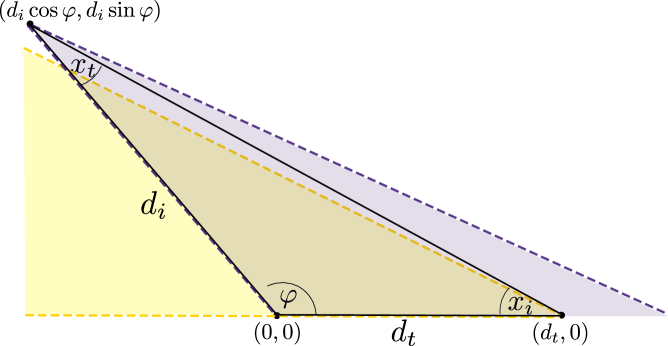
Figure 12: Target STA and potential interferer in the Cartesian plane. The blue area represents the right half of the beam of the potential interference directed towards the AP in $(0,0)$; it has width $\theta_{\rm S}/2$ in correspondence of the potential interferer. Analogously, the yellow area is the upper half of the beam of the target STA. Notice that in this example the two STAs cannot hear each other, since the antenna gain of the target STA in $(d_{i}\cos\varphi,d_{i}\sin\varphi)$ is zero; this means that $\varphi<\varphi_{\lim}(d_{i})$.

Here we prove that STAs in group $n_{I,1}$ have the phase of their polar coordinates in the range $[\varphi_{\rm lim}(d_{i}),2\pi-\varphi_{\rm lim}(d_{i})]$, with $\varphi_{\rm lim}$ given in (23).

Consider a possible interferer at distance $d_{i}\in[0,R]$ from the AP and with angular phase $\varphi\in[0,\pi]$; this means that we are only focusing on the upper half of the circular area around the AP, being the scenario symmetric. Consider the triangle whose vertices are the AP $(0,0)$, the target STA $(d_{t},0)$ and the interferer $(d_{i}\cos\varphi,d_{i}\sin\varphi)$, as in Fig. 12. The two edges that form the vertex coinciding with the AP have length $d_{i}$ and $d_{t}$, and the angle they form has width $\varphi$. Denote the other two angles as $x_{i}$ and $x_{t}$, as in Fig. 12.

We are interested in the angles $\varphi$ such that the target STA is in the beam of the interferer, i.e., $x_{i}\leq\theta_{\rm S}/2$, and the interferer is in the beam of the target STA, i.e., $x_{t}\leq\theta_{\rm S}/2$ (the beams are symmetric with respect to the AP and have width $\theta_{\rm S}$). Moreover, the angles must satisfy the two following equations

$$x_{i}+x_{t}+\varphi=\pi,$$ (33)

$$\frac{d_{i}}{\sin x_{i}}=\frac{d_{t}}{\sin x_{t}}\,,$$ (34)

where (34) comes from the law of sines. If $d_{i}\leq d_{t}$, then $x_{i}\geq x_{t}$, and thus the limit condition is obtained for $x_{i}=\theta_{\rm S}/2$. Considering (33) and (34), we then obtain that we are interested in all angles $\varphi\geq\varphi_{\lim}=\pi-\theta_{\rm S}/2-\arcsin(d_{i}/d_{t}\sin\theta_{\rm S}/2)$. Similarly, when $d_{i}>d_{t}$, the limit condition is obtained for $x_{t}=\theta_{\rm S}/2$, yielding $\varphi_{\lim}=\pi-\theta_{\rm S}/2-\arcsin(d_{t}/d_{i}\sin\theta_{\rm S}/2)$. This proves Eq. (23). Taking into account also STAs in the lower half of the area around the AP, we finally obtain that the other STAs can overhear the messages sent by the target STA if and only if their phase is in $[\phi_{\lim}(d_{i}),2\pi-\phi_{\lim}(d_{i})]$, with $d_{i}$ being their distance from the AP.

Appendix B

Here we explain how to express (27) and (28) so as to compute them in closed form. We focus only on the first of the two integrals in (27), since analogous considerations can be made for the second one, and refer to it as $I_{1}=\int_{0}^{R}\int_{\varphi_{\rm lim}(r)}^{\varphi_{\rm AP}}\partial\theta r\,\partial r.$ $I_{1}$ is zero if $\varphi_{\rm lim}(r)\!>\!\varphi_{\rm AP}$ for the considered $r\in[0,R]$ and position $d_{t}$ of the target node (see (23)). In particular $I_{1}\!=\!0$ if

$$\arcsin\left(c_{1}\sin\frac{\theta_{\rm S}}{2}\right)<\pi-\frac{\theta_{\rm S}}{2}-\varphi_{\rm AP}$$ (35)

with $c_{1}=r/d_{t}$ if $r\leq d_{t}$ and $c_{1}=d_{t}/r$ otherwise (as per (23)). We recall that $0\leq\theta_{\rm S}\leq\pi$ and $0\leq\varphi_{\rm AP}\leq\theta_{\rm AP}\leq\pi$ by assumption. Therefore, denoting the sum $\pi-\theta_{\rm S}/2-\varphi_{\rm AP}$ as $c_{2}$, it is $-\pi/2\leq c_{2}\leq\pi$. Note also that $0\leq c_{1}\sin\theta_{\rm S}/2\leq 1$, yielding $0\leq\arcsin(c_{1}\sin\theta_{\rm S}/2)\leq\pi/2$.

• If $c_{2}\in[\pi/2,\pi]$, then the conditions in (35) are certainly true, yielding $I_{1}=0$. This happens if $\varphi_{\rm AP}<\pi/2-\theta_{\rm S}/2$, whatever the value of $d_{t}$.

• Otherwise $c_{2}\in[-\pi/2,\pi/2]$. In this range the sine function is monotonically increasing, so that it is possible to apply it to both terms in (35) without additional adjustment. This gives the condition $c_{1}\sin\theta_{\rm S}/2<\sin\left(\pi-\theta_{\rm S}/2-\varphi_{\rm AP}\right)$, which can be expressed as $c_{1}<\sin\left(\pi-\frac{\theta_{\rm S}}{2}-\varphi_{\rm AP}\right)/\sin\frac{\theta_{\rm S}}{2}\triangleq c_{3}$. It follows that $I_{1}=0$ if $r<d_{t}c_{3}$ in the case $r\leq d_{t}$ and if $r>d_{t}/c_{3}$ in the case $r>d_{t}$. This happens only if $c_{3}\leq 1$, i.e., $\phi_{\rm AP}<\pi-\theta_{\rm S}$.

Summing up, it is

$$I_{1}=\Bigg{(}\int\limits_{\max(d_{t}c_{3},0)}^{d_{t}}\left(-c_{2}+\arcsin\left(\frac{r}{d_{t}}\sin\frac{\theta_{\rm S}}{2}\right)\right)r\,\partial r$$ (36)

$$+\int_{d_{t}}^{\min(\frac{d_{t}}{c_{3}},R)}\left(-c_{2}+\arcsin\left(\frac{d_{t}}{r}\sin\frac{\theta_{\rm S}}{2}\right)\right)r\,\partial r\Bigg{)}\mathbbm{1}_{\varphi_{\rm AP}\geq\pi-\theta_{\rm S}}$$

with $\mathbbm{1}_{X}$ being the indicator function, equal to $1$ if condition $X$ is true, and to $0$ otherwise. The $\min$ and $\max$ operators in the integral limits ensure that the range $[0,R]$ is not exceeded. Eq. (36) can be solved in closed form: to this aim, it is necessary to evaluate the integration limits where there are the $\max$ and $\min$ operators. The same procedure can be used to compute the second integral $I_{2}$ in (27) using $\theta_{\rm AP}-\varphi_{\rm AP}$ rather than $\varphi_{\rm AP}$.

This expression of ${\mathcal{R}}_{R,C}(d_{t},\varphi_{\rm AP})$ can be used to compute its expectation as in (28). We can focus only on the first double integral (the one over $\phi_{{\rm AP}}$), since analogous considerations can be made on the second one (the one over $\theta_{{\rm AP}}-\phi_{{\rm AP}}$). Such first integral is made over $I_{1}$ and $I_{2}$. We consider only the integral over $I_{1}$ and denote it as $J_{1}$; the rest of the terms in (28) can then be derived following the same approach. It is necessary to characterize $d_{t}/c_{3}$ and $d_{t}c_{3}$ based on $d_{t}$ and $\varphi_{\rm AP}$, so as to remove the min and max operators in the terms in (36). It is $d_{t}c_{3}>0$ if $\varphi_{\rm AP}\leq\pi-c$, and $d_{t}/c_{3}<R$ if $d_{t}\leq Rc_{3}$.

Rigorously from (36), it is $J_{1}=0$ if $\phi_{\rm AP}<\pi-\theta_{\rm S}$. This can be checked beforehand as it only depends on system parameters. It is then possible to evaluate $J_{1}$ in closed form and, repeating the same procedure for the other terms in (28), calculate $\mathrm{E}\left[{\mathcal{R}}_{R,C}\right]$.

References

- [1] IEEE 802.11 WG, “IEEE 802.11ad, amendment 3: Enhancements for very high throughput in the 60 GHz band,” Dec. 2012.
- [2] S. Rangan, T. S. Rappaport, and E. Erkip, “Millimeter-wave cellular wireless networks: Potentials and challenges,” Proceedings of the IEEE, vol. 102, no. 3, pp. 366–385, March 2014.
- [3] T. Nitsche, C. Cordeiro, A. B. Flores, E. W. Knightly, E. Perahia, and J. C. Widmer, “IEEE 802.11ad: directional 60 GHz communication for multi-Gigabit-per-second Wi-Fi,” IEEE Communications Magazine, vol. 52, no. 12, pp. 132–141, Dec. 2014.
- [4] S. Kutty and D. Sen, “Beamforming for millimeter wave communications: An inclusive survey,” IEEE Communications Surveys & Tutorials, vol. 18, no. 2, pp. 949–973, Second Quarter 2016.
- [5] B. Satchidanandan, S. Yau, P. Kumar, A. Aziz, A. Ekbal, and N. Kundargi, “TrackMAC: An IEEE 802.11ad-compatible beam tracking-based MAC protocol for 5G millimeter-wave local area networks,” in International Conference on Communication Systems & Networks (COMSNETS). IEEE, Jan. 2018, pp. 185–182.
- [6] G. Bianchi, “Performance analysis of the IEEE 802.11 distributed coordination function,” IEEE Journal on Selected Areas in Communications, vol. 18, no. 3, pp. 535–547, March 2000.
- [7] A. Akhtar and S. C. Ergen, “Directional MAC protocol for IEEE 802.11ad based wireless local area networks,” Ad Hoc Networks, vol. 69, pp. 49–64, Feb. 2018.
- [8] Q. Chen, J. Tang, D. T. C. Wong, X. Peng, and Y. Zhang, “Directional cooperative MAC protocol design and performance analysis for IEEE 802.11ad WLANs,” IEEE Transactions on Vehicular Technology, vol. 62, no. 6, pp. 2667–2677, July 2013.
- [9] C. Pielli, T. Ropitault, and M. Zorzi, “The potential of mmwaves in smart industry: Manufacturing at 60 GHz,” in International Conference on Ad-Hoc Networks and Wireless. Springer, Sept. 2018, pp. 64–76.
- [10] P. Chatzimisios, A. C. Boucouvalas, and V. Vitsas, “IEEE 802.11 packet delay-a finite retry limit analysis,” in IEEE Global Telecommunications Conference, (GLOBECOM’03), vol. 2. IEEE, Dec. 2003, pp. 950–954.
- [11] J. W. Robinson and T. S. Randhawa, “Saturation throughput analysis of IEEE 802.11e enhanced distributed coordination function,” IEEE Journal on Selected Areas in Communications, vol. 22, no. 5, pp. 917–928, Aug. 2004.
- [12] F.-Y. Hung and I. Marsic, “Performance analysis of the IEEE 802.11 DCF in the presence of the hidden stations,” Computer Networks, vol. 54, no. 15, pp. 2674–2687, Oct. 2010.
- [13] K. Chandra, R. V. Prasad, and I. Niemegeers, “Performance analysis of IEEE 802.11ad MAC protocol,” IEEE Communications Letters, vol. 21, no. 7, pp. 1513–1516, July 2017.
- [14] C. Hemanth and T. Venkatesh, “Performance analysis of contention-based access periods and service periods of 802.11ad hybrid medium access control,” IET Networks, vol. 3, no. 3, pp. 193–203, Sept. 2013.
- [15] M. N. Upama Rajan and A. V. Babu, “Saturation throughput analysis of IEEE 802.11ad wireless LAN in the contention based access period (CBAP),” in IEEE Distributed Computing, VLSI, Electrical Circuits and Robotics (DISCOVER). IEEE, 2016, pp. 41–46.
- [16] F. Babich and M. Comisso, “Throughput and delay analysis of 802.11-based wireless networks using smart and directional antennas,” IEEE Transactions on Communications, vol. 57, no. 5, May 2009.
- [17] M. N. Upama Rajan and A. V. Babu, “Theoretical maximum throughput of IEEE 802.11ad millimeter wave wireless LAN in the contention based access period: With two level aggregation,” in International Conference on Wireless Communications, Signal Processing and Networking (WiSPNET). IEEE, March 2017, pp. 2531–2536.
- [18] H. Shokri-Ghadikolaei, L. Gkatzikis, and C. Fischione, “Beam-searching and transmission scheduling in millimeter wave communications,” in IEEE International Conference on Communications (ICC). IEEE, June 2015, pp. 1292–1297.
- [19] E. Khorov, A. Ivanov, A. Lyakhov, and V. Zankin, “Mathematical model for scheduling in IEEE 802.11ad networks,” in Wireless and Mobile Networking Conference (WMNC). IEEE, July 2016, pp. 153–160.
- [20] W. L. Stutzman and G. A. Thiele, Antenna theory and design. John Wiley & Sons, 2012.
- [21] H. Assasa, S. Kumar Saha, A. Loch, D. Koutsonikolas, and J. Widmer, “Medium access and transport protocol aspects in practical 802.11ad networks,” in 19th International Symposium on ”A World of Wireless, Mobile and Multimedia Networks” (WoWMoM), June 2018.