Searching for Fossil Fields in the Gravity Sector

Abstract

Evidence for the presence of extra fields during inflation may be found in the anisotropies of the scalar and tensor spectra across a vast range of scales. Indeed, beyond the single-field slow-roll paradigm, a long tensor mode can modulate the power spectrum inducing a sizable quadrupolar anisotropy. We investigate how this dynamics plays out for the tensor two-point correlator. The resulting quadrupole stores information on squeezed tensor non-Gaussianities, specifically those sourced by the extra field content and responsible for the breaking of so-called consistency relations. We underscore the potential of anisotropies as a probe of new physics: testable at CMB scales through the detection of B-modes, they are accessible at smaller scales via interferometers and pulsar timing arrays.

I Introduction

The detection of gravitational waves from black hole mergers and from colliding neutron stars Abbott:2016blz has ushered in a new era for astronomy. The same is bound to happen for early universe cosmology upon observing (evidence of) a primordial tensor signal. In particular, probes of the gravity sector hold a great discovery potential when it comes to inflationary physics. Detection of CMB B-modes polarisation would, in standard single-field slow-roll scenarios, precisely identify the energy scale of inflation. Crucially, gravitational probes can access precious information on the early acceleration phase also in the case of multi-field inflation.
A non-minimal inflationary field content is not only possible, but perhaps even likely Baumann:2014nda . String theory realisations of the acceleration mechanism typically result in extra dynamics due, for example, to compactifications moduli. Axion particles as well as Kaluza-Klein modes and gauge fields can also be accommodated. The extra content acts as a source of the standard inflationary scalar and tensor fluctuations. An interesting phenomenology ensues whereby tensor fluctuations, sometimes sourced already at linear order, may deliver a non-standard tensor power spectrum exhibiting a marked scale dependence, features, and in specific cases Anber:2009ua ; Barnaby:2010vf ; Adshead:2012kp ; Dimastrogiovanni:2016fuu ; Pajer:2013fsa ; Garcia-Bellido:2016dkw a chiral signal. Additionally, a similar dynamics is arrived at by employing new (broken) symmetry patterns Endlich:2012pz or so-called non-attractor phases for the inflationary mechanism Ozsoy:2019slf ; Mylova:2018yap .
Perhaps the most sensitive probe of extra physics is the (scalar/tensor/mixed) bispectrum. Its amplitude and momentum dependence can be mapped onto specific properties of the inflationary Lagrangian. Remarkably, the soft momentum limit of the bispectrum contains detailed information Arkani-Hamed:2015bza on the mass, the spin, and (implicitly) the couplings of extra fields. The existence of a non-trivial squeezed bispectrum contribution, mediated by the extra content, may be inferred already at the level of the tensor power spectrum. Indeed, in what we shall call the ultra-squeezed configuration, a long tensor mode induces a position-dependence in the short modes power spectrum. In this context, a non-trivial bispectrum corresponds to one that modifies so-called consistency relations (CRs). These are maps between “soft” limits of N+1-point functions and their lower order counterpart that result from a residual diffeomorphism in the description of the physical system. Standard inflationary CRs are modified in the presence of e.g. non-Bunch-Davies initial conditions, independent modes that transform non-linearly under the diffeomorphism, alternative symmetry breaking patterns, etc Hinterbichler:2013dpa . A prototypical example of modified CRs stems from the presence of extra fields during inflation. Interactions mediated by (see Fig. 1) the extra $\sigma$ content are precisely those that can modify CRs. As a result of CRs breaking, the $\sigma$-mediated leading contribution to the squeezed bispectrum is physical, i.e. it cannot be gauged away.

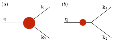
Figure 1: Diagrammatic representation of a tensor three-point function mediated by extra $\sigma$ fields. Red circles indicate interactions between the tensor modes of the metric and $\sigma$ fields. Diagrams leading to a non-trivial consistency-relation-breaking bispectrum are the subset of those in (a) that cannot be simplified to the form in (b). Indeed, the latter diagram is sensitive to information on $\sigma$, which is already probed via the standard tensor two-point function.

In what follows, we analyse the power spectrum of tensor fluctuations in the presence of a long-wavelenth tensor mode as a probe of squeezed tensor non-Gaussianity . The modulation effect can occur at widely different scales, from the CMB all the way to regimes accessible via interferometers. In Sec. II we analyse in detail how the squeezed tensor bispectrum induces a quadrupolar anisotropy in the tensor power spectrum. In Sec. III, building on the recent important works Bartolo:2018evs ; Bartolo:2018rku , we elaborate on the fact that such observable is not plagued by the suppression effects that prevent a direct measurement of tensor non-Gaussianity at interferometer scales. We conclude with Sec. IV.

II Quadrupolar anisotropy

If inflation predicts a non-trivial tensor-scalar-scalar bispectrum in the squeezed limit (the tensor being the soft mode), a quadrupolar anisotropy is induced by the long-wavelength tensor mode in the observed local scalar power spectrum Dai:2013kra . In close analogy to the procedure developed in Dai:2013kra for the scalar case, we now show (see also Ricciardone:2017kre ; Dimastrogiovanni:2018uqy ) that the tensor power spectrum is modulated by a long-wavelength tensor fluctuation. The quadrupolar anisotropy of the tensor power spectrum is then an observable sensitive to the squeezed limit of tensor non-Gaussianity.

The starting point is the correlation between two tensor modes in the presence of a long-wavelength mode. We express the primordial spin-2 tensor fluctuation around a conformally flat, FRW metric in terms of its Fourier modes as

$$\hat{\gamma}_{ij}(\textbf{x},\tau)=\int\frac{d^{3}k}{(2\pi)^{3}}e^{i\textbf{k}\cdot\textbf{x}}\hat{\gamma}_{\textbf{k},ij}(\tau)\,,$$ (1)

adopting the mode decomposition

$$\hat{\gamma}_{\textbf{k},ij}(\tau) =\sum_{\lambda=R,L}\epsilon_{ij}^{\lambda}(\hat{\textbf{k}})\hat{\gamma}_{\textbf{k}}^{\lambda}(\tau)\,,$$ (2)

$$\hat{\gamma}_{\textbf{k}}^{\lambda}(\tau) =a_{\textbf{k}}^{\lambda}\gamma^{\lambda}_{k}(\tau)+a_{-\textbf{k}}^{\lambda\,\dagger}\gamma^{\lambda\,*}_{k}(\tau)\,.$$ (3)

The creation and annihilation operators $a_{\textbf{k}}^{\lambda\,\dagger},\,a_{\textbf{k}}^{\lambda}\,$, satisfy the standard commutation relations. The polarisation tensors $\epsilon_{ij}^{\lambda}(\hat{\textbf{k}})$ are transverse and traceless, are normalised such that $\epsilon_{ij}^{R}(\hat{\textbf{k}})\epsilon_{ij}^{R}(-\hat{\textbf{k}})=\epsilon_{ij}^{L}(\hat{\textbf{k}})\epsilon_{ij}^{L}(-\hat{\textbf{k}})=1$, and moreover $\epsilon_{\ell m}^{R}(-\hat{\textbf{k}})=\epsilon_{\ell m}^{R\,*}(\hat{\textbf{k}})=\epsilon_{\ell m}^{L}(\hat{\textbf{k}})=\epsilon_{\ell m}^{L\,*}(-\hat{\textbf{k}})$. In the absence of significant modulations induced by couplings with long-wavelength modes, the tensor power spectrum and bispectrum – for models that do not violate isotropy nor parity symmetry – are given by

$$\langle\hat{\gamma}_{\textbf{k}_{1}}^{\lambda_{1}}\hat{\gamma}_{\textbf{k}_{2}}^{\lambda_{2}}\rangle\, \equiv \,(2\pi)^{3}\,\delta^{\lambda_{1}\lambda_{2}}\,\delta^{(3)}(\textbf{k}_{1}+\textbf{k}_{2})P^{\lambda_{1}}_{\gamma}(k_{1})\,,$$ (4)

$$\langle\hat{\gamma}^{\lambda_{3}}_{\textbf{q}}\hat{\gamma}_{\textbf{k}_{1}}^{\lambda_{1}}\hat{\gamma}_{\textbf{k}_{2}}^{\lambda_{2}}\rangle \equiv (2\pi)^{3}\delta^{(3)}(\textbf{k}_{1}+\textbf{k}_{2}+\textbf{q})B_{\gamma}^{\lambda_{1}\lambda_{2}\lambda_{3}}(\textbf{k}_{1},\textbf{k}_{2},\textbf{q})\,.$$

The general expression that accounts for modulation due to the coupling with long-wavelength tensor modes is instead Jeong:2012df :

$$\langle\hat{\gamma}_{\textbf{k}_{1}}^{\lambda_{1}}\hat{\gamma}_{\textbf{k}_{2}}^{\lambda_{2}}\rangle_{\gamma_{L}}\,\equiv\,(2\pi)^{3}\,\delta^{\lambda_{1}\lambda_{2}}\,\delta^{(3)}(\textbf{k}_{1}+\textbf{k}_{2})P^{\lambda_{1}}_{\gamma}(k_{1})+$$

$$\sum_{\lambda_{3}}\int_{|\vec{q}|<q_{L}}d^{3}q\,\delta^{(3)}(\textbf{k}_{1}+\textbf{k}_{2}+\textbf{q})\gamma^{*\lambda_{3}}_{\textbf{q}}\,\frac{B_{\gamma}^{\lambda_{1}\lambda_{2}\lambda_{3}}(\textbf{k}_{1},\textbf{k}_{2},\textbf{q})}{P^{\lambda_{3}}_{\gamma}(q)}\,,$$

where $q_{L}$ is a cut-off on whose size we shall soon elaborate. It suffices here to say that it is ensuring we integrate only over the squeezed configurations of the bispectrum $B_{\gamma}$. In standard single-field inflationary models, the leading terms in $B_{\gamma}$ are related to the scale dependence of the (short) tensor power spectrum through consistency relations Maldacena:2002vr . As a result, their effect can be removed by an appropriate gauge transformation (see e.g. Gerstenlauer:2011ti ; Giddings:2011zd ; Dai:2013kra ; Dai:2015rda ; Sreenath:2014nka ). In models where consistency relations are modified or broken, $B_{\gamma}$ accesses directly new physical information stored in the squeezed tensor bispectrum. It is in the case of the latter set of models and, in particular, of their consistency-relation-breaking contributions to the bispectrum, that our analysis becomes especially relevant. It will be convenient in what follows to use the quantity $\tilde{B}$, defined as

$$B_{\gamma}^{\lambda_{1}\lambda_{2}\lambda_{3}}|_{q\ll k_{1,2}}\simeq-\delta^{\lambda_{1}\lambda_{2}}\epsilon_{\ell m}^{\lambda_{3}}(\hat{q})\hat{k}_{1\ell}\hat{k}_{2m}\,\tilde{B}(\textbf{k}_{1},\textbf{k}_{2},\textbf{q})\,,$$ (7)

in order to make the dependence on polarisation indices explicit. The quantity in $\tilde{B}$ can be parametrically large and lead to observable effects. To make the physical consequences of such modulation more manifest, it is useful to express the tensor two point function as

$$\langle\hat{\gamma}_{ij}(\textbf{x}_{1})\hat{\gamma}_{ij}(\textbf{x}_{2})\rangle_{\gamma_{L}}=$$

$$\Big{\langle}\sum_{\lambda_{1},\lambda_{2}}\int\frac{d^{3}k_{1}}{(2\pi)^{3}}e^{i\textbf{k}_{1}\cdot\textbf{x}_{1}}\epsilon_{ij}^{\lambda_{1}}(\hat{\textbf{k}}_{1})\hat{\gamma}_{\textbf{k}_{1}}^{\lambda_{1}}\int\frac{d^{3}k_{2}}{(2\pi)^{3}}e^{i\textbf{k}_{2}\cdot\textbf{x}_{2}}\epsilon_{ij}^{\lambda_{2}}(\hat{\textbf{k}}_{2})\hat{\gamma}_{\textbf{k}_{2}}^{\lambda_{2}}\Big{\rangle}_{\gamma_{L}}$$

$$=\int\frac{d^{3}k_{1}}{(2\pi)^{3}}\,e^{i\textbf{k}_{1}(\textbf{x}_{1}-\textbf{x}_{2})}\,P_{\gamma}(k_{1})+{\cal S}\,,$$ (8)

where $P_{\gamma}=P_{\gamma}^{R}+P_{\gamma}^{L}$. Upon introducing the new coordinates

$$\textbf{k}\equiv\frac{\textbf{k}_{2}-\textbf{k}_{1}}{2}\,,\quad\textbf{p}\equiv\textbf{k}_{1}+\textbf{k}_{2},$$

$$\textbf{x}_{c}\equiv\frac{\textbf{x}_{1}+\textbf{x}_{2}}{2}\,,\quad\textbf{x}\equiv\textbf{x}_{2}-\textbf{x}_{1},$$ (9)

and using $\delta^{(3)}(\textbf{k}_{1}+\textbf{k}_{2}+\textbf{q})=\delta^{(3)}(\textbf{p}+\textbf{q})$, one finds

$${\cal S}= \sum_{\lambda_{1}\lambda_{2}\lambda_{3}}\int\frac{d^{3}k}{(2\pi)^{3}}\frac{d^{3}p}{(2\pi)^{3}}\times$$

$$\,\,\epsilon_{ij}^{\lambda_{1}}\left(\widehat{\frac{\textbf{p}}{2}-\textbf{k}}\right)\epsilon_{ij}^{\lambda_{2}}\left(\widehat{\frac{\textbf{p}}{2}+\textbf{k}}\right)\,e^{i\left(\textbf{p}\cdot\textbf{x}_{c}+\textbf{k}\cdot\textbf{x}\right)}P_{\gamma}(k)$$

$$\times\gamma^{\lambda_{3}\,*}_{-\textbf{p}}\frac{\tilde{B}(\textbf{k},\,\textbf{p})}{P_{\gamma}(k)P_{\gamma}^{\lambda_{3}}(p)}\epsilon^{\lambda_{3}}_{\ell m}(-\hat{p})\hat{k}_{\ell}\hat{k}_{m}\delta^{\lambda_{1}\lambda_{2}}\,$$

$$= \int\frac{d^{3}k}{(2\pi)^{3}}e^{i\textbf{k}\cdot\textbf{x}}P_{\gamma}(k)\,\mathcal{Q}_{\ell m}(\textbf{x}_{c},\,\textbf{k})\hat{k}_{\ell}\hat{k}_{m}\,,$$ (10)

where the anisotropy parameter $\mathcal{Q}_{\ell m}$ is given by

$$\mathcal{Q}_{\ell m}(\textbf{x}_{c},\textbf{k})\equiv\int\frac{d^{3}q}{(2\pi)^{3}}\,e^{i\textbf{q}\cdot\textbf{x}_{c}}\times$$

$$\sum_{\lambda_{3}}\left[\frac{\tilde{B}(\textbf{k},\,\textbf{q})}{(1/2)P_{\gamma}(k)P_{\gamma}^{\lambda_{3}}(q)}\right]\epsilon^{\lambda_{3}}_{\ell m}(-\hat{q})\,\gamma^{*\lambda_{3}}_{-\textbf{q}}$$

$$= \int\frac{d^{3}q}{2\pi^{3}}\,e^{i\textbf{q}\cdot\textbf{x}_{c}}\,f_{\rm nl}(\textbf{q},\textbf{k})\sum_{\lambda_{3}}\epsilon^{\lambda_{3}}_{\ell m}(-\hat{q})\,\gamma^{*\lambda_{3}}_{-\textbf{q}}\;.$$ (11)

Note that in Eq. (II) the following parameterisation $\tilde{B}(\textbf{k},\,\textbf{q})\,=\,f_{\rm nl}(\textbf{q},\textbf{k})\,P_{\gamma}(k)P_{\gamma}(q)$ has been adopted and the usual properties of the polarisation tensors have been used. The quantity $f_{\rm nl}$ parameterises the amplitude and momentum dependence of the squeezed limit of the tensor bispectrum. Going back to Fourier space and expressing $\textbf{x}_{1}$ and $\textbf{x}_{2}$ in terms of x and $\textbf{x}_{c}$, one finds the following expression for the tensor power spectrum in the presence of a long-wavelength tensor mode $\gamma_{\textbf{q}}$, evaluated locally, i.e. within a volume whose linear dimension is smaller than the wavelength of the tensor ($|\textbf{x}|\ll 1/q$):

$$P_{\gamma}(\textbf{k}^{\prime},\textbf{x}_{c})|_{\gamma_{L}}\equiv\int d^{3}x\,e^{-i\textbf{k}^{\prime}\cdot\textbf{x}}\Big{\langle}\hat{\gamma}_{ij}\left(\textbf{x}_{c}-\frac{\textbf{x}}{2}\right)\hat{\gamma}_{ij}\left(\textbf{x}_{c}+\frac{\textbf{x}}{2}\right)\Big{\rangle}_{\gamma_{L}}$$

$$=P_{\gamma}(k^{\prime})\Big{(}1+\mathcal{Q}_{\ell m}(\textbf{x}_{c},\textbf{k}^{\prime})\hat{k}^{\prime}_{\ell}\hat{k}^{\prime}_{m}\Big{)}\,.$$ (12)

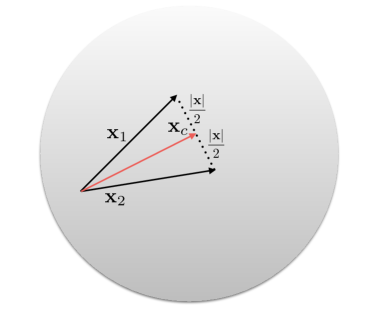
Figure 2: in Eq. (II), for a given point in space $\textbf{x}_{c}$, the volume of integration is defined by a length scale much smaller than the typical variation scale of the modulating tensor mode. If inflation supports a non-zero tensor bispectrum in the squeezed configuration, the power spectrum defined locally, i.e. in the vicinity of $\textbf{x}_{c}$, has a quadrupole modulation caused by long-wavelength tensor fluctuations.

Expanding the quadrupole modulation in spherical harmonics and computing its variance, one arrives at

$$\overline{\mathcal{Q}^{2}}\equiv\Big{\langle}\sum_{m=-2}^{+2}|\mathcal{Q}_{2m}|^{2}\Big{\rangle}=\frac{8\pi}{15}\Big{\langle}\mathcal{Q}_{ij}\mathcal{Q}^{*}_{ij}\Big{\rangle}\,,$$ (13)

and

$$\Big{\langle}\mathcal{Q}_{ij}\mathcal{Q}^{*}_{ij}\Big{\rangle}=16\int\frac{d^{2}\hat{q}}{4\pi}\,\int_{q^{\text{min}}}^{q^{\text{max}}}\frac{dq}{q}f_{\text{nl}}^{2}(\textbf{q},\textbf{k})\mathcal{P}_{\gamma}(q)\,,$$ (14)

where the definition $\mathcal{P}_{\gamma}(q)\equiv q^{3}P_{\gamma}(q)/2\pi^{2}$ has been used. We pause here to comment on how the extrema of integration over $q$ are chosen. The lower value $q^{\text{min}}$ is selected as the wavenumber corresponding to the longest wavelengths that ever exited the horizon. The value of $q^{\text{max}}$ depends instead on the specific probe. For CMB observations, for example, $q^{\text{max}}$ is given by the smallest wavenumber probed by a given experiment. The case of interferometers will be the subject of a more detailed discussion in what follows.
Whenever $f_{\rm nl}$ and the tensor power spectrum ${\cal P}_{\gamma}$ are scale-invariant, Eq. (14) simplifies to

$$\Big{\langle}\mathcal{Q}_{ij}\mathcal{Q}^{*}_{ij}\Big{\rangle}=16f_{\text{nl}}^{2}\,\mathcal{P}_{\gamma}\ln\left(\frac{q^{\text{max}}}{q^{\text{min}}}\right)\,.$$ (15)

Models of (super)solid Ricciardone:2017kre ; Ricciardone:2016lym and non-attractor Ozsoy:2019slf inflation do indeed support in some regimes an (almost) scale invariant profile for both the power spectrum and $f_{\rm nl}$. Let us focus on Eq. (15) in the case of CMB polarisation. Recalling the definition of the tensor-to-scalar ratio as $r\equiv\mathcal{P}_{\gamma}/\mathcal{P}_{\zeta}$, one finds

$$\sqrt{\overline{\mathcal{Q}^{2}}}=2.4\cdot 10^{-4}f_{\text{nl}}\,\sqrt{r\,\Delta N}\,,$$ (16)

where the number of e-folds between the exit of the longest mode $q^{\text{min}}$ and the exit of $q^{\text{max}}$ is $\Delta N\equiv\ln(q^{\text{max}}/q^{\text{min}})$. As an example, with $\Delta N=\mathcal{O}(1)$, a value for $\sqrt{\overline{\mathcal{Q}^{2}}}$ of order $0.1$ requires $f_{\text{nl}}\sqrt{r}\simeq 500$. Given current constraints on the tensor-to-scalar ratio, this demands $f_{\text{nl}}\gtrsim 2\cdot 10^{3}$. Observational bounds on tensor non-Gaussianity have been obtained from temperature and E-mode polarization data for a class of models predicting bispectra that peak in the equilateral configuration Akrami:2019izv : $f_{\text{nl}}^{\text{Planck}}=500\pm 1100\,(68\%\,\text{CL})$, where $f_{\text{nl}}^{\text{Planck}}\equiv B(k,k,k)/[(18/5)P_{\zeta}^{2}(k)]$. These constraints do not immediately apply to our case. However, even if enforced on our set-up, they would be compatible with $f_{\text{nl}}\sqrt{r}=\mathcal{O}(500)$. It would be interesting to forecast the bounds that future CMB polarization experiments will be able to place on squeezed non-Gaussianity by probing the tensor quadrupolar anisotropy. We leave this to future work.

If the tensor power spectrum and/or $f_{\rm nl}$ are not scale invariant, the expression for the quadrupole anisotropy is modified w.r.t. Eq. (15). As a concrete example, let us consider a tensor bispectrum mediated by a massive spin-2 field with a small speed of sound Bordin:2018pca . In this set-up, the power spectrum of gravitational waves receives the standard vacuum contribution and the one generated by the extra field: $P_{\gamma}(k)=[(4H^{2})/(M_{\text{Pl}}^{2}k^{3})](1+\alpha_{\gamma})$. Considering contributions to the bispectrum mediated by the extra particle, for $\alpha_{\gamma}=\mathcal{O}(1)$ one finds Dimastrogiovanni:2018gkl :

$$f_{\text{nl}}\simeq 4\cdot 2^{\nu}\cdot\frac{M_{\text{Pl}}}{H}\cdot\frac{\mu}{H}\cdot\frac{\rho^{3}}{H^{3}}s^{\text{sq}}(\nu,c_{\sigma})\left(\frac{q}{k}\right)^{\frac{3}{2}-\nu}\,,$$ (17)

where $\nu\equiv\sqrt{9/4-m^{2}_{\sigma}/H^{2}}$, with $m_{\sigma}$ the mass of the spin-2 field, and $c_{\sigma}$ its sound speed. The parameters $\mu$ and $\rho$ quantify respectively the magnitude of the cubic self-interaction of the spin-2 field and of the quadratic mixing of the same field with metric tensor modes. In this set-up, for $m_{\sigma}$ of order Hubble, the square root of the quadrupole variance is typically of order $10^{-1}$ on CMB scales. This in spite of the $(q/k)^{3/2-\nu}$ suppression w.r.t. the scale-invariant case. We note here that models with excited initial states (see e.g. Brahma:2013rua ) may also be of particular interest for quadrupolar anisotropies. In some of these constructions $f_{\rm nl}$ scales with negative powers of $q/k$, which may easily lead to a sizable quadrupole.

As the above examples illustrate, the quadrupolar asymmetry corresponding to a scale-dependent spectrum and $f_{\rm nl}$ is model-dependent. If the primordial gravitational wave (GW) spectrum has a sufficiently large amplitude at small scales (see e.g. Bartolo:2016ami for a review of several such scenarios), primordial non-Gaussianity can act as a source for anisotropies of the stochastic GW background. These can be detectable (see Sec. III) both with interferometers and pulsar timing arrays (PTA).

The formalism for the analysis of anisotropies of stochastic gravitational wave backgrounds (SGWBs) measurable with ground and space-based detectors was introduced in Allen:1996gp ; Cornish:2002bh . Techniques developed for PTA can be found in Mingarelli:2013dsa ; Hotinli:2019tpc . These studies are motivated by astrophysical phenomena: anisotropies can for example be associated with groups of unresolved sources on localised regions of the sky, such as large cosmic structures. Similar methods can also be applied in the context of our work, where anisotropies have a primordial origin and ${\cal Q}_{ij}$ is characterised by random matrix entries obeying Gaussian statistics. We shall adopt the notation of the classic work Allen:1997ad . As first discussed in Allen:1996gp , the overlap function $\gamma_{12}$, associated with the cross-correlation of signals measured with a pair of ground-based detectors, receives contributions due to tensor anisotropies. In the vanishing frequency limit, and small antenna regime, we find a simple analytic expression for the correction associated with the quadrupolar anisotropy described by Eq. (II):

$$\gamma_{12}(f\to 0)\,=\,2\,d_{1}^{ij}d_{2\,ij}-\frac{8}{7}{\cal Q}_{ij}\left(d_{1}^{\,im}\,d_{2\,m}^{j}+d_{2}^{\,im}\,d_{1\,m}^{j}\right)\,.$$ (18)

Here $d_{a}^{ij}\,\equiv\,1/2\,\left(\hat{X}_{a}^{i}\hat{X}_{a}^{j}-\hat{Y}_{a}^{i}\hat{Y}_{a}^{j}\right)$ denotes the detector tensor, and ${\hat{X}}_{a}$, $\hat{Y}_{a}$ the interferometer arm directions. At high frequencies, the contributions of the anisotropy to the overlap function are suppressed, and one recovers the results of Allen:1997ad . Anisotropies of SGWBs can then be detected and analyzed through their distinctive effects on a daily modulation of the signal, as first proposed in Allen:1996gp .

One might wonder how to distinguish, when probing interferometer scales, primordial sources of quadrupolar tensor anisotropy from astrophysical ones. We stress that a bispectrum with a large component in the squeezed configuration can induce anisotropies in the GW spectrum both at CMB and at interferometer scales. If the signal is sufficiently large to be measurable by two independent probes, one may search for common properties in the tensor quadrupolar harmonics, which may hint to a primordial origin for the anisotropies. We leave such investigations for future work.

III GW propagation and ultra-squeezed bispectrum

We have seen in Sec. II how a long wavelength tensor mode can induce anisotropies in the power spectrum. At CMB scales the quadrupole serves as an indirect probe of squeezed non-Gaussianity, complementary to direct measurements of three-point correlations of temperature and polarization anisotropies.

Is the same possible at small scales? Two recent works Bartolo:2018evs ; Bartolo:2018rku have shown that primordial tensor non-Gaussianity cannot be probed directly, i.e. by measuring three (or higher, connected) point functions of tensor fluctuations at interferometer scales. Paraphrasing Bartolo:2018evs , measurements of primordial tensor modes correlations at small scales involve angular integrations of contributions from signals produced by a large number of separate, independent, Hubble patches. In light of the central limit theorem, the statistics of tensor perturbations measured at interferometer scales will then be Gaussian. Even in the case of a set of detectors built with the specific purpose of probing a large number of Hubble patches, one would not be able to detect non-Gaussian correlations. Indeed, tensor non-Gaussianity at small scales is suppressed due to Shapiro time-delay effects associated with the propagation of tensor modes at sub-horizon scales in the presence of matter. Reference Bartolo:2018evs suggests that observables sensitive to large correlations between short and long wavelength tensor modes, induced for example by an ultra-squeezed bispectrum, may escape these conclusions. A concrete realisation of such a possibility is precisely the quadrupolar anisotropy of the power spectrum discussed in Sec. II, which relied in part on previous works for the scalar Dimastrogiovanni:2014ina ; Dimastrogiovanni:2015pla and tensor Ricciardone:2017kre ; Dimastrogiovanni:2018uqy ; Ozsoy:2019slf cases. The quadrupolar asymmetry survives the aforementioned cancellation effects because it is induced by a super-horizon tensor fluctuation. As we shall see in some detail, such mode does not experience the sub-horizon evolution responsible for the suppression of the non-Gaussian signal.

III.1 Propagation at sub-horizon scales

We start by reviewing how propagation affects short-wavelength modes Bartolo:2018rku and then apply the same techniques to the case under scrutiny. Their momenta being centered at (ground or space-based) interferometers frequencies, short modes have entered the horizon during the radiation-dominated era. For $k>k_{\text{eq}}$ and $\eta<\eta_{\text{eq}}$, the mode-function reads

$$\gamma_{\textbf{k}}^{\text{RD}}(\eta)=j_{0}(k\eta)\gamma^{\text{prim}}_{\textbf{k}}\,,$$ (19)

where $j_{0}(k\eta)=\sin(k\eta)/(k\eta)$ is the spherical Bessel function and $\gamma_{\textbf{k}}^{\text{prim}}=\gamma_{k}^{\text{prim}}a_{\textbf{k}}+\gamma_{k}^{\text{prim}*}a_{-\textbf{k}}^{\dagger}$ is the primordial tensor perturbation. The initial conditions for $\gamma^{\text{prim}}$ are set by inflation . Eq. (19) has been derived from the the tensor modes equation of motion

$$\gamma_{k}^{\prime\prime}+2\mathcal{H}\gamma_{k}^{\prime}+k^{2}\gamma_{k}=0\,,$$ (20)

by setting $\mathcal{H}=1/\eta$ for the radiation-dominated era.
During matter-domination, and to leading order in $|k\eta|$, one has ,Bartolo:2018rku :

$$\gamma_{\textbf{k}}(\eta)\simeq\frac{1}{(k\eta)^{2}}\left[\mathcal{C}(\textbf{k})\,e^{i\Gamma(\textbf{k},\eta)}+\mathcal{C}^{\dagger}(-\textbf{k})\,e^{-i\Gamma(-\textbf{k},\eta)}\right]\,,$$ (21)

where $\mathcal{C}(\textbf{k})$ is a constant operator and

$$\Gamma(\textbf{k},\eta) = k\eta+2k\int_{\eta_{\text{eq}}}^{\eta}d\eta^{\prime}\Phi(\eta^{\prime},(\eta^{\prime}-\eta_{0})\hat{k})\,.$$ (22)

$$\equiv k\eta+Z(\textbf{k},\,\eta)$$ (23)

with $\Phi$ the Newtonian potential. The above expressions underscore that inhomogeneities in the matter density at small scales – encoded in $\Phi$ – affect the evolution of tensor modes. Matching Eqs.(19) and (21) at the time of matter-radiation equality, $\eta=\eta_{\text{eq}}$, implies

$$\gamma_{\textbf{k}}(\eta_{\text{eq}}) = \frac{\cos(k\eta_{\text{eq}})}{(k\eta_{\text{eq}})^{2}}\left[\mathcal{C}(\textbf{k})+\mathcal{C}^{\dagger}(-\textbf{k})\right]$$ (24)

$$+\frac{\sin(k\eta_{\text{eq}})}{(k\eta_{\text{eq}})^{2}}\left[i\,\mathcal{C}(\textbf{k})-i\,\mathcal{C}^{\dagger}(-\textbf{k})\right]$$

$$=\frac{\sin(k\eta_{\text{eq}})}{(k\eta_{\text{eq}})}\gamma_{\textbf{k}}^{\text{prim}}\,.$$

From Eq. (24) one obtains

$$\mathcal{C}(\textbf{k})=\frac{k\eta_{\text{eq}}}{2i}\gamma_{\textbf{k}}^{\text{prim}}\,.$$ (25)

The solution for $\eta>\eta_{\text{eq}}$ then becomes

$$\gamma_{\textbf{k}}(\eta)\,=\,\frac{\eta_{\text{eq}}}{k\eta^{2}}\left(\frac{e^{i\Gamma(\textbf{k},\eta)}-e^{-i\Gamma(-\textbf{k},\eta)}}{2\,i}\right)\gamma_{\textbf{k}}^{\text{prim}}\,.$$ (26)

Let us now compute the two-point correlation function:

$$\langle\gamma^{\lambda_{1}}_{ij}(\textbf{k}_{1},\eta)\gamma^{\lambda_{2}}_{ij}(\textbf{k}_{2},\eta)\rangle = \frac{\eta_{\text{eq}}^{2}}{\eta^{4}k_{1}k_{2}}\frac{\epsilon_{ij}^{\lambda_{1}}(\hat{k}_{1})\epsilon_{ij}^{\lambda_{2}}(\hat{k}_{2})}{(-4)}$$

$$\times\langle\gamma^{\text{prim}}_{\textbf{k}_{1}}\gamma^{\text{prim}}_{\textbf{k}_{2}}\rangle\cdot\mathcal{E}(\textbf{k}_{1},\textbf{k}_{2},\eta)\,,$$

where

$$\mathcal{E}\equiv\big{\langle}\left(e^{i\Gamma(\textbf{k}_{1},\eta)}-e^{-i\Gamma(-\textbf{k}_{1},\eta)}\right)\cdot\left(e^{i\Gamma(\textbf{k}_{2},\eta)}-e^{-i\Gamma(-\textbf{k}_{2},\eta)}\right)\big{\rangle}\,.$$ (28)

Upon using

$$\langle\gamma^{\text{prim}}_{\textbf{k}_{1}}\gamma^{\text{prim}}_{\textbf{k}_{2}}\rangle=(2\pi)^{3}\delta^{\lambda_{1}\lambda_{2}}\delta^{(3)}(\textbf{k}_{1}+\textbf{k}_{2})P^{\lambda_{1}}(k_{1})\,,$$

$$\epsilon_{ij}^{\lambda_{1}}(\hat{k}_{1})\epsilon_{ij}^{\lambda_{1}}(-\hat{k}_{1})=1\;,$$ (29)

one finds

$$\langle\gamma^{\lambda_{1}}_{ij}(\textbf{k}_{1},\eta)\gamma^{\lambda_{2}}_{ij}(\textbf{k}_{2},\eta)\rangle=$$

$$(2\pi)^{3}\delta^{\lambda_{1}\lambda_{2}}\delta^{(3)}(\textbf{k}_{1}+\textbf{k}_{2})P^{\lambda_{1}}(k_{1})\frac{\eta_{\text{eq}}^{2}}{(-4)\eta^{4}k_{1}^{2}}\,\mathcal{E}(\textbf{k}_{1},-\textbf{k}_{1},\eta)\,.$$

Using Eq. (23), Eq. (28) becomes

$$\mathcal{E} = -2+e^{2ik_{1}\eta}\big{\langle}e^{iZ(\textbf{k}_{1},\eta)}e^{iZ(-\textbf{k}_{1},\eta)}\big{\rangle}$$

$$+e^{-2ik_{1}\eta}\big{\langle}e^{-iZ(-\textbf{k}_{1},\eta)}e^{-iZ(\textbf{k}_{1},\eta)}\big{\rangle}\,.$$

In Eq. (III.1), the expectation values can be computed using the relation Bartolo:2018rku

$$\langle e^{\varphi_{1}}e^{\varphi_{2}}\rangle=e^{\frac{\langle\varphi_{1}^{2}\rangle}{2}+\frac{\langle\varphi_{2}^{2}\rangle}{2}+\langle\varphi_{1}\varphi_{2}\rangle}\,,$$ (32)

which assumes Gaussian statistics for $\varphi$, yielding real exponentials multiplied by $\cos(2k_{1}\eta)$, $\sin(2k_{1}\eta)$ functions. These terms drop out when performing the time average. One is left with the contribution

$$\langle\gamma^{\lambda_{1}}_{ij}(\textbf{k}_{1},\eta)\gamma^{\lambda_{2}}_{ij}(\textbf{k}_{2},\eta)\rangle=$$

$$(2\pi)^{3}\delta^{\lambda_{1}\lambda_{2}}\delta^{(3)}(\textbf{k}_{1}+\textbf{k}_{2})\frac{\eta_{\text{eq}}^{2}}{2\eta^{4}k_{1}^{2}}P^{\lambda_{1}}(k_{1})\,.$$ (33)

We now extend these results and consider the local power spectrum of gravitational waves evaluated in the presence of long-wavelength tensor perturbations, at a generic time $\eta$ during matter domination:

$$\langle\gamma^{\lambda_{1}}_{ij}(\textbf{k}_{1},\eta)\gamma^{\lambda_{2}}_{ij}(\textbf{k}_{2},\eta)\rangle_{\gamma_{L}} = \frac{\eta_{\text{eq}}^{2}}{\eta^{4}k_{1}k_{2}}\frac{\epsilon_{ij}^{\lambda_{1}}(\hat{k}_{1})\epsilon_{ij}^{\lambda_{2}}(\hat{k}_{2})}{(-4)}$$

$$\times \langle\gamma^{\text{prim}}_{\textbf{k}_{1}}\gamma^{\text{prim}}_{\textbf{k}_{2}}\rangle_{\gamma_{L}}\cdot\mathcal{E}(\textbf{k}_{1},\textbf{k}_{2},\eta)\,.$$

Here Eq. (26) has been used and $\langle\gamma^{\text{prim}}_{\textbf{k}_{1}}\gamma^{\text{prim}}_{\textbf{k}_{2}}\rangle_{\gamma_{L}}$ is given by Eq. (II). The standard (isotropic) term in the first line of Eq. (II) produces a contribution identical to the one in Eq. (III.1). The term in Eq. (II) proportional to the squeezed primordial bispectrum becomes instead

$$\langle\gamma^{\lambda_{1}}_{ij}(\textbf{k}_{1},\eta)\gamma^{\lambda_{2}}_{ij}(\textbf{k}_{2},\eta)\rangle_{\gamma_{L}}\supset-\frac{1}{4}\frac{\eta_{\text{eq}}^{2}}{\eta^{4}k_{1}k_{2}}\epsilon_{ij}^{\lambda_{1}}(\hat{k}_{1})\epsilon_{ij}^{\lambda_{2}}(\hat{k}_{2})$$

$$\times\sum_{\lambda_{3}}\int_{|\vec{q}|<q_{L}}d^{3}q\,\delta^{(3)}(\textbf{k}_{1}+\textbf{k}_{2}+\textbf{q})\frac{\gamma^{*\lambda_{3}}_{\textbf{q}}\,B_{\gamma}^{\lambda_{1}\lambda_{2}\lambda_{3}}(k_{1},k_{2},q)}{P^{\lambda_{3}}_{\gamma}(q)}$$

$$\times\mathcal{E}(\textbf{k}_{1},\textbf{k}_{2},\eta)\,.$$ (35)

Let us expand the expectation value in the last line of (III.1) using Eq.(23)

$$\mathcal{E}(\textbf{k}_{1},\textbf{k}_{2}) = \big{\langle}e^{i\left(k_{1}+k_{2}\right)\eta}e^{iZ(\textbf{k}_{1},\eta)}e^{iZ(\textbf{k}_{2},\eta)}$$ (36)

$$+ e^{-i\left(k_{1}+k_{2}\right)\eta}e^{-iZ(-\textbf{k}_{1},\eta)}e^{-iZ(-\textbf{k}_{2},\eta)}$$

$$+ e^{-i\left(k_{1}-k_{2}\right)\eta}e^{-iZ(-\textbf{k}_{1},\eta)}e^{iZ(\textbf{k}_{2},\eta)}$$

$$+ e^{i\left(k_{1}-k_{2}\right)\eta}e^{iZ(\textbf{k}_{1},\eta)}e^{-iZ(-\textbf{k}_{2},\eta)}\big{\rangle}\,.$$

Similarly to what happens for the standard power spectrum, the contributions proportional to $e^{\pm i(k_{1}+k_{2})\eta}$ (first two lines of Eq. 36) average out because of the fast oscillation. Indeed, the period of oscillation, $\sim\pi/k_{1}$, is many orders of magnitude smaller than the integration interval. If we could set $\textbf{k}_{1}=-\textbf{k}_{2}$ the last two terms of (36) would become constant and constitute the only contributions left after averaging over time (as is the case for the standard power spectrum). This is precisely what happens in our context: from Eq. (III.1) we learn that the relation between the wavenumbers is $\textbf{k}_{1}=-\textbf{k}_{2}-\textbf{q}$, with $k_{1}\simeq k_{2}\gg q$. The difference $k_{1}-k_{2}$ is therefore of the order of the inverse cosmic time, $1/\eta_{0}$ ($q$ being at least horizon-size) and the exponentials $e^{\pm i(k_{1}-k_{2})\eta}$ can be treated as constants when performing the time average. Moreover, in the ultra-squeezed configuration ($\textbf{k}_{1}\simeq-\textbf{k}_{2}$) the arguments of the $Z$ terms in the last two lines in (36) are approximately equal and, from Eq. (III.1), one can thus set $\mathcal{E}(\textbf{k}_{1},\textbf{k}_{2})\simeq-2$. It follows that the quadrupolar anisotropy of the tensor spectrum, induced by the ultra-squeezed component of the tensor bispectrum, is not suppressed by propagation effects.

III.2 Averaging

As noted in Bartolo:2018evs , the contributions of a primordial bispectrum to the three-point function of the detector time delay $\Delta\eta(\eta_{0})$, as measured along the interferometer arms, vanishes as a result of rapidly oscillating phases $e^{i{\sum_{i}\pm k_{i}\eta_{0}}}$. This is not the case for the power spectrum: by enforcing $k_{1}=k_{2}$ the rapidly oscillating coefficient drops out Bartolo:2018evs . Let us now include the contribution due to coupling with long-wavelength tensor fluctuations to the time delay two-point function. We find:

$$\langle\Delta\eta(\eta_{0})\Delta\eta(\eta_{0})\rangle \sim \int d^{3}k_{1}d^{3}k_{2}\,e^{i\left(\textbf{x}_{1}\cdot\textbf{k}_{1}+\textbf{x}_{2}\cdot\textbf{k}_{2}\right)}e^{i\left(k_{1}-k_{2}\right)\eta_{0}}$$ (37)

$$\times\mathcal{M}\left(\hat{L}_{1}\cdot\hat{k}_{1},k_{1}\right)\mathcal{M}^{*}\left(-\hat{L}_{2}\cdot\hat{k}_{2},k_{2}\right)$$

$$\times\langle\gamma(\textbf{k}_{1},\eta_{0})\gamma(\textbf{k}_{2},\eta_{0})\rangle_{\gamma_{L}}\,,$$

with ${\cal M}$ the detector transfer function, and $\hat{L}_{i}$ the interferometer arm direction. The expectation value in the last line of Eq. (37) includes, in addition to the diagonal contribution, also the off-diagonal term proportional to the primordial bispectrum in the ultra-squeezed limit. For the ultra-squeezed configuration (with the long-wavelength mode $q$ being at least horizon-sized), one has $|k_{1}-k_{2}|\simeq q$, with $q\leq\eta_{0}^{-1}$ , where $\eta_{0}$ is the cosmic time. As a result, $|k_{1}-k_{2}|\eta_{0}\simeq q\,\eta_{0}\leq 1$ and, similarly to the isotropic contribution, no suppression occurs. The part controlled by the squeezed bispectrum selectively picks up the contribution of signals emitted from the same Hubble patch, without involving correlations from distinct Hubble regions.

We conclude that the quadrupole anisotropy computed in Sec. II propagates all the way to the observed tensor power spectrum, and hence the gravitational waves energy density.

IV Conclusions

The inflationary paradigm stands as one of the main pillars of modern cosmology. This position has been secured in light of its explanatory power on early universe dynamics and the agreement of inflationary predictions with observations. These successes notwithstanding, the current one is only a broad-brush picture of the inflationary mechanism with key questions still unanswered: what is the energy scale of inflation? What about its particle content? The observables that hold the most promise to access such information are the power spectrum and bispectrum of primordial correlation functions, both in the scalar and tensor sectors. The predictions corresponding to the two and three-point functions in the minimal inflationary scenario have long been known. Any observed deviation would therefore point directly to new physics.

Currently available data place strong constraints on the inflationary scalar sector at CMB scales: the power spectrum amplitude and scale dependence are known whilst non-Gaussianity is strongly constrained. The latter may still store key information on the mass, spin, and coupling of the theory field content. Many more unkowns characterise the tensor sector with the predicted primordial signal still undetected and a tensor-to-scalar ratio correspondingly bounded to $r<0.06\,(95\%{\rm CL})$ Akrami:2018odb . The advent of ground and space-based laser interferometers makes it possible to test for inflationary models with a non-standard scale dependence in the power spectrum and search for tell-tale signs of their particle content.

Recent studies Bartolo:2018evs ; Bartolo:2018rku have shown how the signal from one key observable when it comes to probing extra fields, namely the primordial tensor bispectrum, is strongly suppressed at interferometers scales. Among other effects, propagation through structure de-correlates primordial modes of different wavelengths. Accessing the bispectrum directly at interferometer (or e.g. PTA) scales, necessarily implies that all the modes have undergone (a long) sub-horizon evolution. In this work we have put forward a complementary approach: looking for quadrupolar anisotropies in the tensor power spectrum as a probe of the primordial tensor bispectrum. Despite not directly accessing the bispectrum, the quadrupole is nevertheless sensitive to modulations of an horizon-size tensor mode on the GW power spectrum. In this configuration one mode is insensitive to propagation while the remaining two are very similar, thus avoiding an overall strong suppression. Quadrupolar tensor anisotropies can be probed at widely different frequency ranges and are therefore an efficient tool for testing inflationary models that support an ultra-squeezed component of the tensor bispectrum.

V Acknowledgements

We are delighted to thank Valerie Domcke and Toni Riotto for comments on the manuscript, and David Wands for discussions on the subject. GT would also like to thank Nicola Bartolo, Ogan Özsoy, Marco Peloso, Angelo Ricciardone, Toni Riotto for discussions. The work of MF is supported in part by the UK STFC grant ST/S000550/1. The work of GT is partially supported by STFC grant ST/P00055X/1.

References

- (1)
- (2) B. P. Abbott et al. [LIGO Scientific and Virgo Collaborations], Phys. Rev. Lett. 116, no. 6, 061102 (2016) [arXiv:1602.03837]; B. P. Abbott et al. [LIGO Scientific and Virgo Collaborations], Phys. Rev. Lett. 119, no. 16, 161101 (2017) [arXiv:1710.05832].
- (3) D. Baumann and L. McAllister, “Inflation and String Theory,”, Cambridge University Press, [arXiv:1404.2601]
- (4) M. M. Anber and L. Sorbo, Phys. Rev. D 81, 043534 (2010) [arXiv:0908.4089]
- (5) N. Barnaby and M. Peloso, Phys. Rev. Lett. 106, 181301 (2011) [arXiv:1011.1500]
- (6) P. Adshead and M. Wyman, Phys. Rev. Lett. 108, 261302 (2012) [arXiv:1202.2366]
- (7) E. Dimastrogiovanni, M. Fasiello and T. Fujita, JCAP 1701, no. 01, 019 (2017) [arXiv:1608.04216]
- (8) E. Pajer and M. Peloso, Class. Quant. Grav. 30, 214002 (2013) [arXiv:1305.3557]
- (9) J. Garcia-Bellido, M. Peloso and C. Unal, JCAP 1612, no. 12, 031 (2016) [arXiv:1610.03763].
- (10) S. Endlich, A. Nicolis and J. Wang, JCAP 1310 (2013) 011 [arXiv:1210.0569]
- (11) O. Ozsoy, M. Mylova, S. Parameswaran, C. Powell, G. Tasinato and I. Zavala, [arXiv:1902.04976]
- (12) M. Mylova, O. Ozsoy, S. Parameswaran, G. Tasinato and I. Zavala, JCAP 1812 (2018) no.12, 024 [arXiv:1808.10475]
- (13) N. Arkani-Hamed and J. Maldacena, [arXiv:1503.08043]
- (14) K. Hinterbichler, L. Hui and J. Khoury, JCAP 1401, 039 (2014) [arXiv:1304.5527].
- (15) N. Bartolo et al., JCAP 1811 (2018) no.11, 034 [arXiv:1806.02819].
- (16) N. Bartolo, V. De Luca, G. Franciolini, A. Lewis, M. Peloso and A. Riotto, [arXiv:1810.12218].
- (17) N. Bartolo, V. De Luca, G. Franciolini, M. Peloso, D. Racco and A. Riotto, [arXiv:1810.12224].
- (18) L. Bordin, P. Creminelli, A. Khmelnitsky and L. Senatore, JCAP 1810, no. 10, 013 (2018) [arXiv:1806.10587].
- (19) E. Dimastrogiovanni, M. Fasiello, G. Tasinato and D. Wands, JCAP 1902, 008 (2019) [arXiv:1810.08866].
- (20) E. Dimastrogiovanni, M. Fasiello and M. Kamionkowski, JCAP 1602, 017 (2016) [arXiv:1504.05993].
- (21) R. Emami and H. Firouzjahi, JCAP 1510, no. 10, 043 (2015) [arXiv:1506.00958].
- (22) L. Dai, D. Jeong and M. Kamionkowski, Phys. Rev. D 88, no. 4, 043507 (2013) [arXiv:1306.3985].
- (23) E. Dimastrogiovanni, M. Fasiello and G. Tasinato, JCAP 1808, no. 08, 016 (2018) [arXiv:1806.00850].
- (24) A. Ricciardone and G. Tasinato, JCAP 1802, no. 02, 011 (2018) [arXiv:1711.02635].
- (25) D. Jeong and M. Kamionkowski, Phys. Rev. Lett. 108 (2012) 251301 [arXiv:1203.0302].
- (26) J. M. Maldacena, JHEP 0305 (2003) 013 [astro-ph/0210603].
- (27) M. Gerstenlauer, A. Hebecker and G. Tasinato, JCAP 1106 (2011) 021 [arXiv:1102.0560].
- (28) S. B. Giddings and M. S. Sloth, Phys. Rev. D 84 (2011) 063528 [arXiv:1104.0002].
- (29) L. Dai, E. Pajer and F. Schmidt, JCAP 1511, no. 11, 043 (2015) [arXiv:1502.02011].
- (30) V. Sreenath and L. Sriramkumar, JCAP 1410, no. 10, 021 (2014) [arXiv:1406.1609].
- (31) A. Ricciardone and G. Tasinato, Phys. Rev. D 96, no. 2, 023508 (2017) [arXiv:1611.04516].
- (32) Y. Akrami et al. [Planck Collaboration], [arXiv:1905.05697].
- (33) S. Brahma, E. Nelson and S. Shandera, Phys. Rev. D 89, no. 2, 023507 (2014) [arXiv:1310.0471].
- (34) N. Bartolo et al., JCAP 1612 (2016) no.12, 026 [arXiv:1610.06481].
- (35) B. Allen and A. C. Ottewill, Phys. Rev. D 56 (1997) 545 [gr-qc/9607068].
- (36) N. J. Cornish, Class. Quant. Grav. 19 (2002) 1279. [link].
- (37) C. M. F. Mingarelli, T. Sidery, I. Mandel and A. Vecchio, Phys. Rev. D 88 (2013) no.6, 062005 [arXiv:1306.5394].
- (38) S. C. Hotinli, M. Kamionkowski and A. H. Jaffe, [arXiv:1904.05348].
- (39) B. Allen and J. D. Romano, Phys. Rev. D 59 (1999) 102001 [gr-qc/9710117].
- (40) E. Dimastrogiovanni, M. Fasiello, D. Jeong and M. Kamionkowski, JCAP 1412, 050 (2014) [arXiv:1407.8204].
- (41) M. Maggiore, Phys. Rept. 331, 283 (2000) [gr-qc/9909001].
- (42) Y. Akrami et al. [Planck Collaboration], [arXiv:1807.06211].
- (43)