The Mathematical Specification
of the
Statebox Language

Contributors

This document is the result of years of discussion, joint work and development by different members of the Statebox team. Ideas, help and feedback from our advisors and many other people met in many different circumstances (at conferences, on the internet, etc.) have also been invaluable and fundamental.

Jelle Herold is to be credited with the original idea of building a programming language based on Petri nets and category theory. Fabrizio Genovese took care of formalizing this idea into a mathematically precise framework, and materially wrote the majority of this document. He is to blame for any typo or inaccuracy in what follows. Many other people contributed in laying down these mathematical foundations, either by proving results or by suggesting central ideas, most notably: Jelle Herold, David Spivak, Neil Ghani, Daniël van Dijk and Stefano Gogioso.

We also want to explicitly thank former and current team members Alex Gryzlov, Fredrik Nordvall-Forsberg, Jack Ek, Marco Perone, André Videla, Andre Knispel, Erik Post, Anton Livaja, Bert Span, Ryan Wisnesky and Anthony Di Franco for the useful technical discussions and material they provided, which made this document better.

Emi Gheorghe, Anton Livaja and Erik Post have to be credited for having done the majority of proofreading of this text.

Acknowledgements

In addition to this, we want to thank all the researchers working in areas related to what we do. They all contributed, either directly or indirectly, by making this document more mathematically grounded. Many of them also dedicated time to our project by taking part in our research meetings and summits, by hosting us at their research institutions and homes or by providing opportunities for us to join community conferences and workshops. This includes many people in the Applied Category Theory community, in particular Pawel Sobocinski, Neil Ghani, Robin Piedeleu, Jules Hedges, David Spivak, Brendan Fong, Jade Master, Fabio Gadducci, Philipp Zahn, Viktor Winschel, Bob Coecke, John Baez, Bas Spitters, Helle Hvid Hansen, Christina Vasilakopoulou, Fabio Zanasi, Bartosz Milewski, Dan Ghica, Christian Williams, David Reutter, Michael Robinson, Francisco Rios, Blake Pollard, Daniel Cicala, and Dusko Pavlovic, as well as people coming from different research fields, such as Andrew Polonsky, Yoichi Hirai, Arian van Putten, Jason Teutsch, Aron Fischer, Jon Paprocki and Martin Lundfall.

Furthermore, we need to thank many of the active members in our online communities (Telegram, Twitter, etc.), which provided conceptual insights, spotted typos, and gave any sort of feedback. We know some of these people only by their digital handles, so we will refer to them in this way when no alternatives are possible: Zans, @no_identd, Hjörvar, Matthew York, Dotrego, Nikolaj-K, Arseniy Klempner, Herve Moal. Special thanks go to Kasper Keunen and Josh Harvey, which provided early feedback and insights and to Roy Blackstone and Greedy Ferengi, which proofread our document and spotted errors.

As one can see this document is the result of many different, entangled contributions. We are sure we forgot to mention some people, and we apologize in advance for this.

In this setting, talking about contribution and ownership in a traditional sense is difficult. For this reason, we opted to use the wording “Statebox team” to broadly refer to the authors and contributors of this paper.

How to cite this document

Statebox Team. The Mathematical Specification of the Statebox Language, 2018. ArXiv: TBD.

Chapter 1 Introduction

This document defines the mathematical backbone of the Statebox language. In the simplest way possible, Statebox can be seen as a clever way to tie together different theoretical structures to maximize their benefits and limit their downsides. Since consistency and correctness are central requisites for our language, it became clear from the beginning that such tying could not be achieved by just hacking together different pieces of code representing implementations of the structures we wanted to leverage: Rigorous mathematics is employed to ensure both conceptual consistency of the language and reliability of the code itself. The mathematics presented here is what guided the implementation process, and we deemed very useful to release it to the public to help people wanting to audit our work to better understand the code itself.

1.1 What to expect

This document is a work in progress, and will be released together with each version of the Statebox language, suitably expanded to cover the new features we will gradually implement. Each version of it will contain more theoretical material than what will actually be implemented in the Statebox version it comes together with. This serves the purpose of helping the audience understand what we are working on, and what to expect from the upcoming releases.

In this document there is very little code involved, and quite a lot of mathematics. The maths will always be introduced together with intuitive explanations meant to clarify the ideas we are trying to formalize. Notice that here we care more about giving the bigger picture of the language itself and will focus on technical details only when strictly needed. There are a number of seminal papers that explain, with a much greater deal of precision, some of the theoretical material that we are employing to implement the Statebox language, and we will constantly refer the reader to them for details. On the other hand, sometimes the material covered here is genuinely new, in which case details can be found in papers we published ourselves in peer reviewed venues, as in [13]. Again, in this case we will reference the audience to our own contributions for a thorough presentation of the concepts covered.

All in all, the reader should consider this document as a high-level presentation of how concepts we are using interact together, and should follow the references provided to understand the technicalities.

• The audience with a strong background in theoretical computer science can use this document to understand how we plan to use results in different research fields to create a new programming language, and how we achieve consistent interaction between them, especially when they are expressed using very different formalisms. An exhaustive explanation of the concepts presented, if needed, will be found in the bibliographic references;

• The inexperienced reader will be able to understand the content of cutting-edge research that would be otherwise difficult or impossible to access directly. Hopefully, reading this document will make the reader’s attempt to read the papers firsthand easier – if they choose to do so.

It is also worth stressing that we did our best to keep the bibliography to a bare minimum, to help the people willing to dig deeper focus on a few, selected resources. In particular, when possible, we relied on works which are considered the standard reference in their field, as in the case of [18] for category theory.

1.2 Prerequisites

We did our best to make this document as accessible as possible. This clearly required a trade-off between exhaustive presentation and conceptual accessibility. In general, we assume very little previous knowledge. Our ideal reader knows some basic set theory, knows how to manipulate equalities and, at least in principle, understands how coding works. This does not mean that it is necessary to be a programmer to understand this document. What we require is having a vague idea of how, conceptually, humans instruct machines on how to perform tasks. This said, an inclination toward logical thinking and approaching problems rationally and in a pragmatic way is surely needed to understand this work properly.

Throughout this document, we will often make remarks and examples intended for a more experienced audience. These are marked with an asterism superscript (like this^$\star$) and can be safely ignored without undermining the general comprehension of the concepts exposed if too difficult to grasp.

We moreover tried as much as possible to stick to common mathematical notation to avoid any kind of discomfort, making exceptions only when ambiguity could arise.

1.3 Synopsis

We conclude this short introduction by presenting a synopsis of what we are going to do in each Chapter of this document. As we already mentioned, this document is a work in progress, and its synopsis will be changed accordingly as the amount of released material grows.

• This document is divided into parts. Part I is named “first concepts” and introduces the basic ideas behind Statebox;

  • In Chapter 2 we will introduce Petri nets, one of the fundamental ingredients in our language. The emphasis in this Chapter falls on why Petri nets make a great graphical tool to reason about complex infrastructure. We will also describe some of the most interesting properties that nets can have, and why it is important to study them;

  • In Chapter 3 we will introduce category theory, the mathematical framework that will allow us to find a common ground to tie Petri nets with other theoretical structures. This will ultimately enable us to export Petri nets from the realm of theoretical research to true software engineering, turning them into a great way of designing complex code while guaranteeing consistency and reliability. The categories we use come endowed with a diagrammatic formalism which we will explain in detail. It will serve the purpose of backing up the strength of mathematical reasoning with a visual, intuitive representation of concepts;

  • In Chapter 4 we will give a first "categorification" of nets, expressing some of the concepts covered in Chapter 2 using category theory. We will show how this allows us to use Petri nets in a much more powerful way and to fine-tune our reasoning about them, for instance by allowing us to track the whole history of a token in a net. This will give us the needed tools to see nets as deterministic objects by defining their categories of executions, which is a fundamental step to make the implementation of Petri nets useful;

  • In Chapter 5 we will elaborate on the results of Chapter 4, showing how we can map Petri nets to other programming languages to produce actual software in a conceptually layered fashion. This is achieved by a functorial mapping from net executions to semantic categories of functional programming languages, allowing us to achieve a separation between software topology and software meaning;

• More parts will follow in the upcoming months, as our research becomes stable enough to be added to this document.

Throughout the document, often at the end of a chapter, we will make direct reference to our codebase to point out how we implemented in practice a mathematical concept. We hope this will help the reader to establish links between the theory presented here and the codebase hosted on Github [30].

Chapter 2 Petri nets

Petri nets were invented by Carl Adam Petri in 1939 to model chemical reactions [25]. In the subsequent years, they have met incredible success, especially in computer science, to study and model distributed/concurrent systems [23, 26]. In this Chapter, we will start explaining what a Petri net is, and why we chose this structure to be at the very core of Statebox.

We will start with an informal introduction, relying on the graphical formalism of nets to present concepts in an intuitive way. Then we will proceed by formalizing everything in mathematical terms. Finally, we will define some useful properties of nets which we will be interested in studying later on.

2.1 Petri nets, informally

A Petri net is composed of places, transitions and arcs weighted on the natural numbers. Any place contains a given number of tokens, which represent resources. Transitions are connected to places through the arcs, and can turn resources into other resources: A transition can fire, consuming tokens living in places connected to its input, and producing tokens living in places connected to its output. An example of a Petri net is shown in Figure 2.1, where:

Figure 2.1: Example of a Petri net.

• Places are represented by blue circles;

• Tokens are represented by black dots in each circle;

• Transitions are represented by gray rectangles;

• A weighted directed arc going from a place to a transition represents the transition input; the weight signifies the number of consumed tokens. To avoid clutter, we omit the weights when they are equal to 1;

• A weighted directed arc going from a transition to a place represents the transition output; the weight signifies the number of produced tokens. To avoid clutter, we omit the weights when they are equal to 1.

A Petri net should be thought of as representing some sort of system. Tokens are resources, and places are containers that hold resources of a given type. Transitions are processes that convert resources from one type to another. Weights on the arcs identify how many resources of some kind a process needs to be executed, and how many resources of some other kind will be produced when the process finishes. With respect to this, we say that a transition can be in two states:

Enabled,

if, in all the places having edges towards the transition, there is a number of tokens at least equal to the weight of the edge itself (see Figure 2.2(a)). Note that if a transition has no inbound edges (as in Figure 2.2(b)), then it is always considered enabled;

Disabled,

otherwise (see Figure 2.2(c)).

(a) Enabled transition.

(b) Trivially enabled transition.

(c) Disabled transition.

Figure 2.2: Example of enabled and disabled Petri nets.

When a transition is enabled, then we say that it may fire. Firing represents the act of executing the process the transition represents. When a transition fires, a number of tokens are removed from each input place, according to the arc weight, and similarly a number of tokens are added to each output place, again according to the arc weight. Figure 2.3 shows an enabled transition before (left) and after (right) firing. As you can see, we highlight firing transitions with a black triangle.

Figure 2.3: An enabled transition before (left) and after (right) firing.

Remark 2.1.1 (Generalized nets).

Note that the behavior of Petri nets can be generalized much further than this, for example by annotating the arcs with logical conditions that have to be satisfied to consider a transition enabled, or by introducing transitions that – a bit counterintuitively – fire only when there are no tokens in one of their input places. Working in a greater degree of generality, though, can make much more difficult – or even impossible – to answer questions pertaining reachability and absence/presence of deadlocks, which are important concepts that will be formally introduced later. In Statebox, the fundamental requirement is that we should always be able to tell what is going on in our processes. For this reason we do prefer working with a restricted set of rules and to be very careful in adopting any generalization. The study of how suitably extend the expressivity of the nets considered here will be the focus of the second part of this document.

2.2 Multisets

The first concrete goal of this Chapter is to state the intuitive concepts presented above in mathematical terms. Before we can introduce Petri nets formally, we need a way to formalize multisets. Intuitively, a multiset is just a set with repetition, meaning that each element is allowed to occur multiple times in the same set. To make things easier to understand, consider the following writings:

$$\{a,b,d,e,k\}\qquad\{a,b,b,d,e,e,e,k\}\qquad\{a,b,b,d,e,e,k,k\}$$ (2.1)

When seen as sets, the ones above denote the same thing, since sets ignore repeated elements. The reason why we are interested in the concept of a multiset is precisely because, in our case, we want to be able to consider the three sets above as distinct. The experienced reader will have already noted how the need for multisets naturally arises when dealing with Petri nets. Specifically, multisets will be useful in:

• Describing the transitions of a Petri net, since we can represent how many tokens a transition consumes (produces) from (in) a place as the number of occurrences of that place in a multiset;

• Describing the state of a Petri net, since we can represent the number of tokens in each place as the number of occurrences of that place in a multiset.

Without further ado, let us introduce the first mathematical definition of this document.

Definition 2.2.1 (Multiset).

A multiset on $S$ is a function ${X}^{\mathbb{N}}_{S}:S\to\mathbb{N}$, where $S$ is a set. A multiset is called finite when there is only a finite number of $s\in S$ such that ${X}^{\mathbb{N}}_{S}(s)>0$. Finite multisets will usually be denoted with a $\mathbb{N}$ used as superscript. For instance, ${X}^{\mathbb{N}}_{S}$ represents a finite multiset on $S$.

Remark 2.2.2 (Non-finite multisets).

In this work, we are only interested in finite multisets. To avoid clutter, we will refer to finite multisets just as multisets.

Example 2.2.3 (Multisets are functions).

As we said, multisets have to be interpreted as sets where the same element can be repeated a finite number of times. If we go back to the sets displayed in Equation 2.1, we readily see how these can indeed be expressed as functions $f,g,h:\{a,b,d,e,k\}\to\mathbb{N}$, taking values:

$$f(a) =1 \qquad f(b) =1 \qquad f(d) =1 \qquad f(e)= 1 \qquad f(k) =1$$

$$g(a) =1 \qquad g(b) =2 \qquad g(d) =1 \qquad g(e)= 3 \qquad g(k) =1$$

$$h(a) =1 \qquad h(b) =2 \qquad h(d) =1 \qquad h(e)= 2 \qquad h(k) =2$$

Where $f$ is the function representing the first multiset, $g$ the function representing the second, and $h$ the function representing the third, respectively.

Remark 2.2.4 (Same multiset, different functions).

Note that our definition of $\mathbb{N}$ includes $0$, and hence if we have a function $g^{\prime}:\{a,b,c,d,e,k\}\to\mathbb{N}$ defined as:

$$g^{\prime}(a) =1 \quad g^{\prime}(b) =2 \quad g^{\prime}(c) =0 \quad g^{\prime}(d) =1 \quad g^{\prime}(e)= 3 \quad g^{\prime}(k) =1$$

This also defines the multiset $\{a,b,b,d,e,e,e,k\}$, like $g$. This can be a source of confusion, and hence in the notation for multiset – namely ${X}^{\mathbb{N}}_{S}$ – we make the base set explicit. Also note that subsets of a set $S$ correspond to functions $f:S\to\{0,1\}$, and can thus be seen as particular multisets on $S$ where each element is mapped to $0$ or $1$.

Definition 2.2.5 (Set of multisets over $S$).

${S}^{\oplus}$ denotes the set of all possible finite multisets over $S$, that is,

$${S}^{\oplus}:=\{{X}^{\mathbb{N}}_{S}:S\to\mathbb{N},\mid\text{${X}^{\mathbb{N}}_{S}(s)>0$ for a finite number of $s\in S$}\}$$

2.2.1 Operations on multisets

To be able to proficiently use multisets to formalize Petri nets, we need to understand what we can do with them. Given two multisets ${X}^{\mathbb{N}}_{S},{Y}^{\mathbb{N}}_{S}$ on $S$, we can generalize many operations from sets to multisets, as inclusion, union and difference using point-wise definitions.

Definition 2.2.6 (Operations on multisets).

Let ${X}^{\mathbb{N}}_{S},{Y}^{\mathbb{N}}_{S}\in{S}^{\oplus}$. Set inclusion generalizes easily setting, for all $s\in S$,

$${X}^{\mathbb{N}}_{S}\subseteq{Y}^{\mathbb{N}}_{S}:={X}^{\mathbb{N}}_{S}(s)\leq{Y}^{\mathbb{N}}_{S}(s)$$

Similarly, union can be generalized to multisets ${X}^{\mathbb{N}}_{S}$ and ${Y}^{\mathbb{N}}_{S}$, setting:

$$\cup:{S}^{\oplus}\times{S}^{\oplus} \to{S}^{\oplus}$$ (2.2)

$$({X}^{\mathbb{N}}_{S}\cup{Y}^{\mathbb{N}}_{S})(s) :={X}^{\mathbb{N}}_{S}(s)+{Y}^{\mathbb{N}}_{S}(s)$$

When ${X}^{\mathbb{N}}_{S}\subseteq{Y}^{\mathbb{N}}_{S}$, we can moreover define their multiset difference, that unsurprisingly is just:

$$-:{S}^{\oplus}\times{S}^{\oplus} \to{S}^{\oplus}$$

$$({Y}^{\mathbb{N}}_{S}-{X}^{\mathbb{N}}_{S})(s) :={Y}^{\mathbb{N}}_{S}(s)-{X}^{\mathbb{N}}_{S}(s)$$

Another intuitive operation that can be defined on multisets is the one of scalar multiplication, that is similar in concept to scalar products for vector spaces. For each $n\in\mathbb{N}$ and $s\in S$, we set:

$$\cdot:\mathbb{N}\times{S}^{\oplus} \to{S}^{\oplus}$$

$$(n\cdot{X}^{\mathbb{N}}_{S})(s) :=n\,{X}^{\mathbb{N}}_{S}(s)$$

Denoting with $S_{1}\sqcup S_{2}$ the disjoint union of sets, that we recall being defined as:

$$S_{1}\sqcup S_{2}:=\{(s_{1},0)\mid s_{1}\in S_{1}\}\cup\{(s_{2},1)\mid s_{2}\in S_{2}\}$$

We can moreover define the analogous disjoint union of multisets, setting for all $s\in S\sqcup S^{\prime}$:

$$\sqcup:{S}^{\oplus}\times{S^{\prime}}^{\oplus} \to{S\sqcup S^{\prime}}^{\oplus}$$

$$({X}^{\mathbb{N}}_{S_{1}}\sqcup{Y}^{\mathbb{N}}_{S_{2}})(s) :=\begin{cases}{X}^{\mathbb{N}}_{S_{1}}(s_{1})\text{ iff }s=(s_{1},0)\\ {Y}^{\mathbb{N}}_{S_{2}}(s_{2})\text{ iff }s=(s_{2},1)\end{cases}$$

For each set $S$ we denote with $\emptyset_{S}$ the multiset in ${S}^{\oplus}$ with the following property:

$$\forall s\in S,~{}\emptyset_{S}(s)=0$$

Finally, we define the cardinality of a multiset ${X}^{\mathbb{N}}_{S}$ as:

$$\left|{X}^{\mathbb{N}}_{S}\right|:=\sum_{s\in S}{X}^{\mathbb{N}}_{S}(s)$$

Remark* 2.2.7 (Multisets are free commutative monoids).

The reader fluent in algebra will have noted that multiset union defines an operation in the algebraic sense, that makes ${S}^{\oplus}$, for each $S$, the free commutative monoid generated by $S$, where the unit is the multiset $\emptyset_{S}$.

Remark* 2.2.8 (Injections of multisets).

The multiset $\emptyset_{S_{1}}$ can be cleverly used to inject ${S_{2}}^{\oplus}$ into ${S_{1}\sqcup S_{2}}^{\oplus}$, as follows:

$${S_{2}}^{\oplus} \hookrightarrow{S_{1}\sqcup S_{2}}^{\oplus}$$

$${Y}^{\mathbb{N}}_{S_{2}} \mapsto\emptyset_{S_{1}}\sqcup{Y}^{\mathbb{N}}_{S_{2}}$$

The set $S$ may be embedded into ${S}^{\oplus}$ via a function $\delta:S\to{S}^{\oplus}$, defined as:

$$\delta(s)(s^{\prime}):=\begin{cases}1,\text{ iff }s=s^{\prime}\\ 0,\text{ iff }s\neq s^{\prime}\\ \end{cases}$$

Finally, given a function $f:S_{1}\to{S_{2}}^{\oplus}$, we can abuse notation and consider $f$ as a function of multisets ${S_{1}}^{\oplus}\to{S_{2}}^{\oplus}$, by defining

$$f:{X}^{\mathbb{N}}_{S_{1}}\in{S_{1}}^{\oplus}\mapsto\bigcup_{s_{1}\in S_{1}}{X}^{\mathbb{N}}(s_{1})\cdot f(s_{1})\in{S_{2}}^{\oplus}$$

In the remainder of this document, we will just write ${X}^{\mathbb{N}}$ instead of ${X}^{\mathbb{N}}_{S}$ when the base set $S$ is clear from the context.

2.3 Petri nets, formally

Now that we have some intuition about how Petri nets work and have introduced multisets, it is time to define Petri nets formally.

Definition 2.3.1 (Petri net).

A Petri net is a quadruple

$$N:=(P_{N},T_{N},{{}^{\circ}}(-)_{N},{(-)_{N}^{\circ}})$$

Where:

• $P_{N}$ is a finite set, representing places;

• $T_{N}$ is a finite set, representing transitions;

• $P_{N}$ and $T_{N}$ are disjoint: Nothing can be a transition and a place at the same time;

• ${{}^{\circ}}(-)_{N}:T_{N}\to{P_{N}}^{\oplus}$ is a function assigning to each transition the multiset of $P_{N}$ representing its input places;

• ${(-)_{N}^{\circ}}:T_{N}\to{P_{N}}^{\oplus}$ is a function assigning to each transition the multiset of $P_{N}$ representing its output places.

We will often denote with $T_{N},P_{N},{{}^{\circ}}(-)_{N},{(-)_{N}^{\circ}}$ the set of places, transitions and input/output functions of the net $N$, respectively.

Example 2.3.2 (Input and output places).

In Figure 2.4 we highlighted the action of ${{}^{\circ}}(t)_{N}$ in red for two different transitions, denoted with $t$. We did the same for ${(t)_{N}^{\circ}}$, highlighted in green.

Figure 2.4: Examples of input/output places of transitions.

Remark* 2.3.3 (Generalized input and output).

Given a Petri net $N$, we can generalize ${{}^{\circ}}(-)_{N}$ and ${(-)_{N}^{\circ}}$ to functions of multisets ${T_{N}}^{\oplus}\to{P_{N}}^{\oplus}$ using the procedure explained in Remark 2.2.8, that is, we can extend them so that they act on multisets of transitions, as follows:

$${{}^{\circ}}(-)_{N}:{U}^{\mathbb{N}}\in{T_{N}}^{\oplus}\mapsto\bigcup_{t\in T_{N}}{U}^{\mathbb{N}}(t)\cdot{{}^{\circ}}(t)_{N}\in{P_{N}}^{\oplus}$$

$${(-)_{N}^{\circ}}:{U}^{\mathbb{N}}\in{T_{N}}^{\oplus}\mapsto\bigcup_{t\in T_{N}}{U}^{\mathbb{N}}(t)\cdot{(t)_{N}^{\circ}}\in{P_{N}}^{\oplus}$$

2.3.1 Markings, enabled transitions

Up to now, we still did not formalize the concept of a marking. At the moment, our Petri nets are empty, meaning that we do not have a way to populate places with tokens. This can be readily expressed using multisets again.

Definition 2.3.4 (Marking).

Given a Petri net $N$, a marking (also called a state) for $N$ is a multiset on $P_{N}$, ${X}^{\mathbb{N}}:P_{N}\to\mathbb{N}$.

The interpretation is that the marking assigns a finite, positive or zero number of tokens to each place of $N$. We denote that a net $N$ comes endowed with a marking ${X}^{\mathbb{N}}$ using the notation $N_{X}^{\mathbb{N}}$. Equivalently, we can also say that $N$ is in the state ${X}^{\mathbb{N}}$ to refer to $N_{X}^{\mathbb{N}}$.

Having formalized the concept of a marking, we can now take care of defining the dynamics of a Petri net.

Definition 2.3.5 (Enabled transition).

Given a Petri net $N$ in the state ${X}^{\mathbb{N}}$, we say that a transition $t\in T_{N}$ is enabled if:

$${{}^{\circ}}(t)_{N}\subseteq{X}^{\mathbb{N}}$$

Note that since we are working with multisets, this is equivalent to

$$\forall p\in P_{N},\,{{}^{\circ}}(t)_{N}(p)\leq{X}^{\mathbb{N}}(p)$$

meaning, as we would expect, that a transition is enabled if and only if in any input place for $t$ there are at least as many tokens available as $t$ will have to consume.

Remark* 2.3.6 (Enabled check).

${P_{N}}^{\oplus}$ denotes the set of all possible multisets over $P_{N}$. For a net $N$ we can define a function

$$\overline{(-)}_{(-)}:T_{N}\times{P_{N}}^{\oplus}\to\{\top,\bot\}$$

that takes a transition $t$ and a marking ${X}^{\mathbb{N}}$ as input and returns $\top$ if $t$ is enabled in ${X}^{\mathbb{N}}$, and $\bot$ otherwise. This function can be generalized to sets of transitions $U\subseteq T_{N}$ by setting $\overline{U}_{{X}^{\mathbb{N}}}:=\bigwedge\limits_{t\in U}\overline{t}_{M}$, where $\bigwedge$ denotes the usual logical conjunction of predicates. This function is important from an implementation point of view as it allows for an efficient way to determine if a given transition can fire in a given state.

2.3.2 Firing semantics for Petri nets

Now, we have to define a firing policy – also called firing semantics – by mathematically formalizing what happens when a transition fires. Given a Petri net $P$ in the state ${X}^{\mathbb{N}}$, the firing of a transition $t$ should have two properties:

• $t$ should be able to fire only when enabled;

• Firing $t$ should consume some tokens and produce others, thus changing the state of $P$ from ${X}^{\mathbb{N}}$ to some other marking ${Y}^{\mathbb{N}}$. We will indicate this using the notation $N_{X}^{\mathbb{N}}\xrightarrow{t}N_{Y}^{\mathbb{N}}$.

These two requirements can be captured by the following definition.

Definition 2.3.7 (Firing rule).

Let $N$ be a Petri net in a state ${X}^{\mathbb{N}}$, and let $t\in T_{N}$. We define:

$$N_{X}^{\mathbb{N}}\xrightarrow{t}N_{Y}^{\mathbb{N}}:=\left({{}^{\circ}}(t)_{N}\subseteq{X}^{\mathbb{N}}\right)\,\wedge\,\left({(t)_{N}^{\circ}}\subseteq{Y}^{\mathbb{N}}\right)\,\wedge\,\left({X}^{\mathbb{N}}-{{}^{\circ}}(t)_{N}={Y}^{\mathbb{N}}-{(t)_{N}^{\circ}}\right)$$

and say that $t$ fires, carrying $N$ from ${X}^{\mathbb{N}}$ to ${Y}^{\mathbb{N}}$, if it is $N_{X}^{\mathbb{N}}\xrightarrow{t}N_{Y}^{\mathbb{N}}$.

Note that in Definition 2.3.7 the requirements ${{}^{\circ}}(t)_{N}\subseteq{X}^{\mathbb{N}}$ and ${(t)_{N}^{\circ}}\subseteq{Y}^{\mathbb{N}}$ are redundant, since ${X}^{\mathbb{N}}-{{}^{\circ}}(t)_{N}$ and ${Y}^{\mathbb{N}}-{(t)_{N}^{\circ}}$ are defined only under such assumption. We decided to list them explicitly to elucidate the fact that for $N_{X}^{\mathbb{N}}\xrightarrow{t}N_{Y}^{\mathbb{N}}$ to be true, $t$ has to be enabled in $N_{X}^{\mathbb{N}}$.

Our firing policy says that, given a place $p\in P_{N}$, when a transition fires, exactly ${{}^{\circ}}(t)_{N}(p)$ tokens are consumed from $p$, and exactly ${(t)_{N}^{\circ}}(p)$ tokens are produced in $p$. This causes the net to go from the state ${X}^{\mathbb{N}}$ to the state ${Y}^{\mathbb{N}}$, where ${Y}^{\mathbb{N}}$ is obtained from ${X}^{\mathbb{N}}$ by adding/subtracting the relevant number of tokens as prescribed by the input and output functions evaluated on $t$.

Note that the same transition can produce and consume tokens from the same places, that is, a place can act both as an input and an output – they are not mutually exclusive. The net in Figure 2.5 is an example of this, where ${{}^{\circ}}(t)_{N}\cap{(t)_{N}^{\circ}}$ is non-empty.

Figure 2.5: An example of a transition with intersecting input and output places.

Remark* 2.3.8 (Generalized firing policy).

Our firing policy can of course be generalized to arbitrary sets of transitions $U\subseteq T_{N}$, defining things in the obvious way:

$$N_{X}^{\mathbb{N}}\xrightarrow{U}N_{Y}^{\mathbb{N}}:={{}^{\circ}}(U)_{N}\subseteq{X}^{\mathbb{N}}\,\wedge\,{(U)_{N}^{\circ}}\subseteq{Y}^{\mathbb{N}}\,\wedge\,{X}^{\mathbb{N}}-{{}^{\circ}}(U)_{N}={Y}^{\mathbb{N}}-{(U)_{N}^{\circ}}$$

2.4 Examples

Petri nets are good for representing the development stage of a product, and concurrent behavior. We will show this using examples.

Figure 2.6: Product development example.

Example 2.4.1 (Product development).

We can describe the life stages of a product, from order to production, using Petri nets. The simplest case we can think of is the one in Figure 2.6. In this case, transitions correspond to different processing stages for a product. Clearly, we can design processes that are much more complicated than this, for instance introducing exclusive choices as in the Petri net in Figure 2.7, where the two transitions must compete to fire. Here we can imagine that a user can decide which transition fires, maybe by pressing a button or by filling in a form. And with this model we can represent the fact that once one decision is taken the other one is automatically disabled.

Figure 2.7: Petri net modeling exclusive choice.

Example 2.4.2 (Traffic Light).

Concurrent behavior models situations where two or more systems have to compete to get the needed resources to run. One typical example is given by a couple of traffic lights (denoted $1$ and $2$, respectively) at a crossing: For simplicity, each traffic light can be green or red, but they cannot be both green at the same time, otherwise cars might crash. We can model this using Petri nets (see Figure 2.8(a)), where two systems – representing the traffic lights – have to compete for the token in the middle to turn the light to green.

In Figure 2.8(a), the places have been colored in red and green, representing “the colour a traffic light is in”. Transitions represent the switches that change a given traffic light’s color. The numbers labeling places represent the traffic light that each place refers to.

Note that with the marking provided as in the figure above, it can never happen that both lights are green at the same time, thanks to the token in the center place: One light, say $1$, could always be “better” at becoming green, thus preventing the second one to ever fire, but situations causing crashes would never happen. Note moreover that since there could be more than one token in each place, there are other markings that do not prevent this situation from happening, such as the one in Figure 2.8(b).

(a) An example of a traffic light model.

(b) An example of a faulty state of the traffic light model.

Figure 2.8: Traffic light models.

2.5 Further properties of Petri nets

Now that we have defined Petri nets formally and clarified why we deem them useful, it is time to explore the properties that a Petri net can have, and to state them formally.

2.5.1 Reachability, safeness and deadlocks

Let us go back to Example 2.4.2. We already saw two different markings, generating two completely different behaviors, in Figure 2.8. We recognize that, in Figure 2.8(b), firing both transitions at the bottom leads us to the marking in Figure 2.9. …But this is exactly the situation we wanted to avoid, since now cars might start crashing! This prompts a question: Given some marking ${X}^{\mathbb{N}}$, is it possible to reach a marking ${Y}^{\mathbb{N}}$ with a sequence of transition firings?

Figure 2.9: The evolution of a faulty state of the traffic light model.

The traffic light example should clarify how important answering this question is. As usual, something important deserves a definition.

Definition 2.5.1 (Reachability).

Given a Petri net $N_{X}^{\mathbb{N}}$ we say that a marking ${Y}^{\mathbb{N}}$ is reachable from ${X}^{\mathbb{N}}$ if there is a finite sequence of transitions $t_{0},...,t_{n}$ such that

$${X}^{\mathbb{N}}\xrightarrow{t_{0}}{X}^{\mathbb{N}}_{1}\xrightarrow{t_{1}}\dots\xrightarrow{t_{n-1}}{X}^{\mathbb{N}}_{n}\xrightarrow{t_{n}}{Y}^{\mathbb{N}}$$

If $s$ is a finite sequence of transitions $(t_{0},...,t_{n})$, we express the statement above by simply writing ${X}^{\mathbb{N}}\xrightarrow{s}{Y}^{\mathbb{N}}$.

Remark 2.5.2 (Studying reachability).

In the traffic light example our Petri net is simple enough to allow us to manually deduce if some marking can be reached from its initial state by writing out all the possible states of the net. Clearly, when we start designing complex systems, we want to develop formal tools to automatically provide answers to this question. This will be covered later on.

Another important concept is the one of deadlock. The idea behind this is that a net is deadlocked if “it is going to jam”, meaning that at some point nothing will be able to fire anymore. This can be formalized as follows:

Definition 2.5.3 (Deadlock).

Given a Petri net $N$ in the state ${X}^{\mathbb{N}}$, we say that $N_{X}^{\mathbb{N}}$ is deadlocked if there is some marking ${Y}^{\mathbb{N}}$, reachable from ${X}^{\mathbb{N}}$, in which no transition can fire.

Example 2.5.4 (Deadlocked net).

In Figure 2.2(c) it is very easy to see that the net is deadlocked, but things are not always so clear. Consider, for instance, Figure 2.10(a) on the left: Here everything seems fine, but firing $t_{2}$ and then $t_{1}$ two times gets us to the state in Figure 2.10(b) on the right, which is deadlocked. Deadlock is undesirable because it means that our process cannot progress in any way. As in the case of reachability, we want to develop higher order tools to study if a given Petri net is deadlocked or not.

(a)

(b)

Figure 2.10: An example of a deadlocked Petri net.

On the other end of the spectrum, opposed to the concept of deadlock, we have the concept of liveness. Liveness means, in short, absence of deadlocks, as it can be easily seen from the following definition:

Definition 2.5.5 (Liveness).

Given a Petri net $N_{X}^{\mathbb{N}}$, we say that a transition $t\in T_{N}$ is

• Dead if it can never fire;

• Alive if, for any marking ${Y}^{\mathbb{N}}$ reachable from ${X}^{\mathbb{N}}$, there is a firing sequence that, from ${Y}^{\mathbb{N}}$, leads to a marking ${Z}^{\mathbb{N}}$ in which $t$ can be fired.

We say that $N_{X}^{\mathbb{N}}$ is alive if all of its transitions are alive.

This in particular means that, starting from $N_{X}^{\mathbb{N}}$, we can apply any firing sequence and be sure that, if we keep going, we will always end up in a situation in which $t$ can fire.

Remark 2.5.6 (Dead and alive are not incompatible).

Note that a transition can be both not dead and not alive at the same time: It may be fireable in the state ${X}^{\mathbb{N}}$ but become dead later on. The definition above can be generalized, introducing intermediate degrees of liveness between the ones we gave above, but we are not interested in this right now. What is interesting for us is that it is trivial to prove that an alive Petri net is not deadlocked, and that every transition will always be enabled in the future, no matter what we do.

Example 2.5.7 (Traffic light nets are alive).

The traffic light nets provided in Figure 2.8 are both alive, while the net in Figure 2.2(c) is not, consisting only of a dead transition.

Being deadlocked is considered a bad quality for a Petri net to have. Another property, called boundedness, is instead considered good:

Definition 2.5.8 (Boundedness and safeness).

Given a Petri net $N_{X}^{\mathbb{N}}$, we say that a place $p\in P_{N}$ is $k$-bounded if it never contains more than $k$ tokens in any reachable marking. We also say that a place is bounded if it is $k$-bounded for some $k$.

We can extend these definitions to the whole net saying that $N_{X}^{\mathbb{N}}$ is $k$-bounded (bounded) if all its places are $k$-bounded (bounded) in any state reachable from ${X}^{\mathbb{N}}$. Finally, we say that a Petri net is safe if it is $1$-bounded.

Example 2.5.9 (Traffic light nets are bounded).

The nets in Figure 2.8 are both bounded. The one in Figure 2.8(a) is also safe.

If we think about Petri nets as modeling process behavior, boundedness is a desirable quality because it means that at any stage tokens do not accumulate. For example, consider the net in Figure 2.6: This net is not bounded, because the leftmost transition could keep firing accumulating tokens in the leftmost place. This would happen if, for instance, the firing rate of the leftmost transition exceeds the firing rate of the middle one, meaning that the demand exceeds the production capability.

Figure 2.11: An example of a bounded Petri net modeling production.

Remark 2.5.10 (Making a net bounded).

Note that in a situation like the one in Figure 2.6 we can make the net $k$-bounded artificially by adding a place with $k$ tokens in it, as in Figure 2.11, where we just made the net above $6$-bounded. The interpretation of the added place is that it represents the maximum production capabilities of the process. In this case the “request” transition is automatically disabled (i.e. it cannot fire) when there are six or more tokens waiting for production.

As usual, we would like a theoretical framework to establish when a net is bounded, or when strategies like the one above can work to make it such. Many of the questions asked here will be answered formally with the categorification of Petri nets, that will unveil their compositional nature.

Figure 2.12: A way to convert a string to a Petri net, and vice-versa.

2.6 Implementation

At the moment, we are implementing Petri nets on different parts of our stack, from frontend to core, using a plethora of different languages. We are also building parsers that allow us to import Petri nets designed in widespread editors such as GreatSPN [33]. This is important since it allows users to design nets in the editor they like the most, and also to use whatever model checking features such editors provide.

Since Petri nets are a bit all over the place in our codebase, and many of the repositories where we are carrying this work are yet to be made open, it is probably better to focus on how we manage to “pass Petri nets around” between different components of our stack. We obtain this by means of serializing/deserializing a net.

With serializing/deserializing a Petri net we mean that we need a way to pass around the information needed to define a Petri net between machines, and to do so we need a procedure to convert this information into an actual net and vice-versa. Considering the very nature of computer networking, this means that we need a way to convert a net to a string, and back. This is shown in Figure 2.12.

The procedure is quite self-explanatory, but we will try to comment on that nevertheless: We start with a string of numbers, where $0$ is treated as a special character. Scanning the string, we chop it every time we encounter a zero. What we are left with now is a bunch of substrings, which we sequentially group into couples. Each of these couples defines input and output of a transition, and as we see this is enough information to build a Petri net.

With this procedure we are able to convert Petri nets to strings and viceversa, and exchange them between components such as, say, the frontend codebase displaying the net to the user and the core codebase dealing with processing net firings in a formally consistent way. As we will see in Section 4.7, this exchange format has the advantage of being able to exchange not only nets, but the categories defining their histories, which we will introduce in Chapter 4.

2.7 Why is this useful?

This is a perfectly legitimate question, that deserves a prompt answer. We will proceed by analytically listing the ways in which Petri nets can be useful for software-design purposes. We hope to give the reader reason to believe that Petri nets are, in fact, a good formalism to base a programming language on. In introducing Petri nets, we pointed out the following characteristics that make them very appetible for software-design purposes:

• Petri nets are inherently graphical. Since the very beginning, we were able to introduce and manipulate Petri nets diagrammatically. The pictorial representation of Petri nets is intuitive, and allows us to quickly draft how a complex system is supposed to work. This makes designing infrastructure with Petri nets much easier than by, say, using traditional code;

• Petri nets represent concurrency well. The idea of transitions having to “fight” for resources is very useful in representing processes that could be run independently on those resources. Again, this can be easily represented graphically, giving us a neat, intuitive explanation of what is going on. Such a feature is of great value in modeling complex systems, often consisting of multiple, independent parties performing concurrent operations on different machines;

• Petri nets can be studied formally. The graphical formalism we rely on to model systems is backed up by a sound mathematical model. This guarantees that our drawings are not just drawings, but that computers can “understand” our drawings by means of the corresponding mathematics;

• Interesting properties of nets can be expressed in terms of reachability. Since reachability is formally defined, we can develop technical tools to infer if a given condition holds or not for a net. This, in particular, means that we can ask a computer to answer such questions for us. If the possibility of algorithmically deciding if some property holds or not for a given net may not seem very important, it is because all the examples provided up to now consisted of very small nets. The reader should be aware that in production applications, Petri nets can easily have many hundreds of places/transitions, and answering reachability questions without the aid of a computer is basically impossible. Clearly, up to now we do not know how efficient algorithms can be in solving such problems, and indeed verifying some properties can take an exponential time (or even worse) in the size of the net. This means that as our net grows in size the time needed to know if some property holds or not for it will increase exponentially. This prompts for the development of efficient methods, such that when an efficient solution to answer a question exists, it is attained.

We decided to use Petri nets as the language that Statebox uses to design code at the highest level of abstraction. More precisely, the programmer will be able to use Petri nets to draft how the software should behave by modeling it as a process, and then dive into details by filling in all the remaining information by means of a well defined procedure, backed up by sound mathematics to ensure consistency of such method. We call this way of writing code behavioral programming. A tutorial about how to employ this technique to write programs can be found in [11].

As this is the direction we want to take, we need a way to recast the Petri nets formalism in a way that makes it compatible with other mathematical gadgets we want to use for the “filling the blanks” stage we mentioned above. This will be done with the aid of category theory, that we will introduce in the next Chapter.

Chapter 3 Introduction to category theory

In Chapter 2 we introduced Petri nets, and definined some of their properties. Now we proceed by introducing the other main actor in the Statebox project, category theory. Category theory is a relatively young branch of mathematics that originated during the second half of the last century [10], and since then it has had an increasingly pervasive influence in the way modern mathematicians and computer scientists think. Category theory can be seen as “the glue of mathematics” and has the marvelous ability of making different theories interact consistently with each other. Set theory is also a universal language for mathematics, with the difference that while sets focus on defining a structure “imperatively” – e.g. by specifying which properties the elements of a structure need to satisfy – category theory defines mathematical structures behaviorally, that is, by specifying patterns and interactions of a structure with structures of similar kind. In this sense, it is clear how working from a categorical perspective makes studying the interaction of different theories easier.

Since one of the main characteristics of the Statebox project is unification of advancements in very different fields of computer science, the reader can already appreciate why category theory will end up being very relevant for us. Indeed, the standard modus operandi of this document will most often reduce to the following pattern:

• Introduce a new idea;

• Find a mathematical theory that captures the idea well;

• Categorify it, that is, translate it to the language of category theory;

• Study how what we obtained interacts with what we already had. One of the main advantages of category theory is that its extensive toolbox makes this step much easier.

Albeit having just sketched out why category theory will have a central role in the development of our theoretical framework, we already have what we need to introduce it in all of its glory. The reader should employ this Chapter as a reference, and not worry too much if something explained here initially does not seem very “useful”. Eventually, every detail will find its place in the environment we are building up.

3.1 What is category theory?

That is a great question – in many ways the answer deepens every day. Category theory is primarily a way of thinking, more than just a theory in the usual sense of the term. Probably the simplest idea of category theory is that everything is interrelated. This applies not only to mathematics, but also computation, physics, and other sciences which are just beginning to be elucidated and unified via the use of categories – and is precisely the reason why category theory has such natural real-world applications. Of course the pertinent application here is in the context of computer science, and the mission of Statebox is to make programming concrete, principled, and universal. First, we begin with a simple mathematical overview of category theory.

According to [19], a nice way to describe category theory is as the language for describing and observing patterns in mathematics. Every object is of a certain kind, which is interrelated by a morphism intrinsic to the kind. For example, a morphism of sets is simply a function, while a morphism of structured objects cooperates with the structure, e.g. an algebraic operation. Taken together, the objects and morphisms form a category, which encapsulates the particular notion, and more so, connects it to all of mathematics – the category is itself a kind of object, and we can consider the category of categories! The morphisms between categories, called functors, respect the composition of morphisms in the related categories, providing a fundamental connection between distinct concepts. A functor witnesses how the reasoning patterns found in a certain theory are “compatible” with the patterns found in another. This entails a well-behaved notion of compatibility between different theories, an essential aspect of principled theoretical modeling called compositionality. In a way, this perspective already empowers us when thinking about mathematics as a whole. But let us slow down and see the basic definitions.

Definition 3.1.1 (Category).

A category $\mathcal{C}$ consists of

• A collection of objects, denoted as $\operatorname{Obj}\,\mathcal{C}$;

• A collection of morphisms, denoted as $\operatorname{Hom}_{\,\mathcal{C}}$;

• Two functions $\operatorname{s}(-),\operatorname{t}(-):\operatorname{Hom}_{\,\mathcal{C}}\to\operatorname{Obj}\,\mathcal{C}$ called source (or domain) and target (or codomain), respectively;

• A partial function $(-);(-):\operatorname{Hom}_{\,\mathcal{C}}\times\operatorname{Hom}_{\,\mathcal{C}}\to\operatorname{Hom}_{\,\mathcal{C}}$, called composition, that assigns to every pair $f,g\in\operatorname{Hom}_{\,\mathcal{C}}$, such that $s(g)=t(f)$, the arrow $f;g$;

• An identity function $\operatorname{Obj}\,\mathcal{C}\to\operatorname{Hom}_{\,\mathcal{C}}$, that assigns to every object $A$ an arrow $id_{A}$.

Moreover, we require that the following axioms have to be satisfied:

• $\operatorname{s}(f)=\operatorname{s}(f;g)$ and $\operatorname{t}(f;g)=\operatorname{t}(g)$;

• $\operatorname{s}(id_{A})=A=\operatorname{t}(id_{A})$;

• $f;(g;h)=(f;g);h$ for each $f,g,h$ arrows such that composition is defined;

• $f;id_{\operatorname{t}(f)}=f=id_{\operatorname{s}(f)};f$ for each arrow $f$.

An arrow $f$ such that $\operatorname{s}(f)=A,\operatorname{t}(f)=B$ is often denoted with $f:A\to B$ or $A\xrightarrow{f}B$.

The concept of category is a very powerful one, and we redirect the reader who wants to know more to [18]: Category theory can indeed become very difficult to grasp only with the introduction of its simplest concepts, and this document is not the right place for an in-dept exposition. Nevertheless, it is worth to give an intuitive explanation of the definition provided above: Objects can be thought of as representing systems, resources, or states of a machine. Arrows represent transformations between them, that is, processes that turn a given system (or resource, or state) into another according to some rules. Moreover, composition tells us that transformations can be serialized: Transforming $A$ into $B$ using $f$ and then $B$ into $C$ using $g$ is the same as transforming $A$ into $C$ using $f;g$. The axioms tell us that composing transformations is associative, and moreover that for each system $A$ “doing nothing” can be regarded as an identity transformation $id_{A}$.

Remark 3.1.2.

In interpreting objects as states of a system and morphisms as transformations between them, we already see some similarity with the interpretation we gave of Petri nets in Chapter 2. This similarity will be described in depth in Chapter 4.

Example 3.1.3 (Sets and functions).

There is a category, denoted with Set, whose objects are sets and whose morphisms are functions between them. It is easy to see that composition of functions is a function, composition is associative, and that every set has an identity function carrying every element into itself. Hence Set is indeed a well-defined category.

Remark 3.1.4 (Notation).

From now on, we will stick to the convention of indicating generic categories with curly letters, like $\mathcal{C},\mathcal{D},\mathcal{E}$. Objects will be denoted with capital Latin letters, preferably from the beginning of the alphabet, $A,B,C$ etc. Morphisms will be denoted with lower-case Latin letters, preferably from the middle of the alphabet, $f,g,h$ etc. Categories that deserve a name of their own, like the one in Example 3.1.3, will have the name denoted in bold letters, as in Set.

Example* 3.1.5 (Functional programming).

We can build a category Hask where objects are data types and morphisms are Haskell [15] functions from one type to another. Associativity is composition of functions, and identity morphisms are the algorithms sending terms to themselves. Defining the category Hask is actually not as easy as it seems and we will discuss more about this issue in Remark 5.2.5.

Example* 3.1.6 (Groups, topological spaces).

Groups and homomorphisms between them form a category, called Group. So do topological spaces and continuous functions, forming the category Top.

Remark* 3.1.7 (Free categories from graphs).

There is an evident connection between the definition of a category and the definition of a graph. A category just looks like “the transitive closure of a graph, with loops added at every vertex”. This connection between categories and graphs is indeed real, and one can always generate a free category from a directed graph [18, Ch. 2, Sec. 7].

Remark* 3.1.8 (Size issues).

The reader with experience in mathematics will have noted how we have been vague in saying what we mean by “a collection of objects” in the definition of a category. Indeed, note how the objects of the category Set, Group and Top do not form a set, but a proper class. All these size issues are deeply covered in any comprehensive book about category theory, and we refer the reader to [18, Ch. 1, Sec. 6] for details.

(a) $f;g=h$.

(b) $h;g=f;k$.

(c) Commutativity of squares ensures commutativity overall.

Figure 3.1: Examples of commutative diagrams.

Remark 3.1.9 (Commutative diagram).

A neat way to express equations between morphisms in a category is via commutative diagrams. A commutative diagram is just a picture that shows us how morphisms compose with each other. Commutative diagrams are interpreted as follows: Vertexes are objects in a category. Paths between objects are compositions of morphisms. If there are multiple paths from one object to another, this means that the corresponding morphisms are equal. For example, the diagram in Figure 3.1(a) states that $f;g=h$, while the diagram in Figure 3.1(b) states that $h;g=f;k$.

Commutative diagrams are a fundamental tool in category theory, and are routinely used to prove things. The standard way to prove something in category theory is to draw a diagram representing our thesis, and then try to prove that the diagram commutes. A way to do this is by dividing the diagram into multiple sub-diagrams and proving the commutativity of each of them separately. The commutativity of the overall diagram can then be inferred by the commutativity of its components. To see how this works, consider Figure 3.1(c): If we know that the left and right squares commute, then so does the rectangle obtained from their composition, in fact:

$$f_{1};g_{1};g_{2}=(f_{1};g_{1});g_{2}=(h_{1};f_{2});g_{2}=h_{1};(f_{2};g_{2})=h_{1};(h_{2};f_{3})=h_{1};h_{2};f_{3}$$

where the second equality follows from the commutativity of the left square, while the fourth follows from the commutativity of the right one.

To conclude this Section, we introduce the concept of isomorphism. Intuitively, an isomorphism in a category is a morphism that allows us “to go back and forth between two objects”. This is easily defined as follows:

Definition 3.1.10 (Isomorphism).

Given a category $\mathcal{C}$ we say that a morphism of $\mathcal{C}$ $f:A\to B$ is an isomorphism (or just an iso) if there is a morphism $f^{-1}:B\to A$ such that

$$f;f^{-1}=id_{A}\qquad f^{-1};f=id_{B}$$

The definition of isomorphism is nothing new, and captures the idea of a “reversible process”. We already know examples of this:

Example 3.1.11 (Isos in Set).

In Set, the isomorphisms are exactly the bijective functions.

Example* 3.1.12 (Isos in Group and Top).

In Group, the isomorphisms are exactly the bijective homomorphisms. In Top, the isomorphisms are exactly the homeomorphisms.

3.2 Functors, natural transformations, natural isomorphisms

We mentioned functors en passant in the introduction of this Chapter, when we said that a functor is a morphism between categories. We moreover added that a morphism in a category can be thought of as a transformation that preserves all the relevant structure from its domain to its codomain. So, if a functor is a morphism of categories, which is the relevant structure it has to preserve?

Well, in a general category the only things that we have are identities for each object and composition of morphisms, so it seems reasonable to require these to be preserved by a functor. This is, indeed, enough:

Definition 3.2.1 (Functor).

A functor $F$ from a category $\mathcal{C}$ to a category $\mathcal{D}$, often denoted with $F:\mathcal{C}\to\mathcal{D}$ or $\mathcal{C}\xrightarrow{F}\mathcal{D}$, consists of the following:

• A map from $\operatorname{Obj}\,\mathcal{C}$ to $\operatorname{Obj}\,\mathcal{D}$, that associates to the object $A$ of $\mathcal{C}$ the object $FA$ of $\mathcal{D}$;

• A map from $\operatorname{Hom}_{\,\mathcal{C}}$ to $\operatorname{Hom}_{\,\mathcal{D}}$, that associates to the morphism $f:A\to B$ of $\mathcal{C}$ the morphism $Ff:FA\to FB$ of $\mathcal{D}$.

• We moreover require that the following equalities hold:

  $$F_{id_{A}}=id_{FA}\qquad F(f;g)=Ff;Fg$$ (3.1)

In particular, Equations 3.1 mean that identities get carried to identities and compositions to compositions, as we would have expected. Note how this is enough to guarantee that $F$ sends any commutative diagram in $\mathcal{C}$ to a commutative diagram in $\mathcal{D}$. This is the whole point about functors: If the main way to prove facts in category theory is by using commutative diagrams, a functor is basically sending facts about $\mathcal{C}$ to facts about $\mathcal{D}$. This allows us to “export” theorems from one category to another, and is a tremendously powerful feature to carry results across mathematical theories.

Example 3.2.2 (Identity functor).

For each category $\mathcal{C}$ there is a functor $id_{\mathcal{C}}$ that sends each object and each morphism of $\mathcal{C}$ to itself, respectively.

Example* 3.2.3 (Homotopy groups).

There is a functor from the category of pointed topological spaces and homotopy classes of continuous functions, $\textbf{hTop}\star$, to the category Group. This is exactly what makes it possible to deduce if a given topological space is connected or not – studying its homotopy group.

Remark 3.2.4 (Functor composition).

Given two functors $\mathcal{C}\xrightarrow{F}\mathcal{D}\xrightarrow{G}\mathcal{E}$ we can compose them by composing their maps on objects and morphisms. The composition sends an object $A$ of $\mathcal{C}$ to an object $FGA$ of $\mathcal{E}$, and a morphism $f:A\to B$ in $\mathcal{C}$ to $FGf:FGA\to FGB$ in $\mathcal{E}$.

Remark 3.2.5 (Notation).

It is commonplace to denote functors using capital Latin letters from the middle of the alphabet, $F,G,H$ etc. Also, the application of a functor to an object or a morphism is usually written without using parentheses, as in $FA,Ff$.

We can now start playing with the definition of functor a bit more. First, something simple:

Definition 3.2.6 (Isomorphism of categories).

Using Remarks 3.2.2 and 3.2.4 it is not difficult to convince ourselves that categories and functors form the objects and morphisms, respectively, of a category, called Cat. Then we can apply Defintion 3.1.10 in this context and obtain that the two categories $\mathcal{C}$ and $\mathcal{D}$ are isomorphic when there are functors $F:\mathcal{C}\to\mathcal{D}$ and $F^{-1}:\mathcal{D}\to\mathcal{C}$ such that $F;F^{-1}=id_{\mathcal{C}}$ and $F^{-1};F=id_{\mathcal{D}}$.

The definition of isomorphism between categories is not really the interesting one for us. This is because it is too restrictive. However, we can relax it a little to make it more manageable. To do this, we first need to introduce some properties.

Definition 3.2.7 (Full and faithful functors).

A functor $F:\mathcal{C}\to\mathcal{D}$ is called full if, for any objects $A,B$ in $\mathcal{C}$ and any morphism $f:FA\to FB$ in $\mathcal{D}$, there is always a morphism $g$ in $\mathcal{C}$ such that $Fg=f$.

On the other hand, $F$ is called faithful if given morphisms $f,g:A\to B$ in $\mathcal{C}$, $f\neq g$ implies $Ff\neq Fg$ in $\mathcal{D}$.

When a functor is full and faithful, we sometimes say that it is fully faithful.

In essence, a functor $F:\mathcal{C}\to\mathcal{D}$ is full when every morphism between objects of the form $FA$, $FB$ – that is, objects that are hit by $F$ – comes from $\mathcal{C}$. This means that the morphisms $A\to B$ are at least as many as the morphisms $FA\to FB$. Similarly, faithfulness implies that the morphisms $FA\to FB$ are at least as many as the ones $A\to B$, since different morphisms from $A$ to $B$ go to different morphisms from $FA$ to $FB$. When a functor is fully faithful, then, all the morphisms between objects of $\mathcal{C}$ are carried to $\mathcal{D}$ exactly as they are, and all the objects of the form $FA$ for some $A$ in $\mathcal{C}$, together with their morphisms, form “a copy” of $\mathcal{C}$ in $\mathcal{D}$.

This is pretty close to an equivalence of categories, but in $\mathcal{D}$ there could be other objects that are not hit by $F$, viz. objects that cannot be written as $FA$ for some $A$ in $\mathcal{C}$. Since these objects are not hit by $F$ they could behave as they want to, while the structure of objects of type $FA$ and their morphisms is completely determined by $\mathcal{C}$ and the full faithfulness of $F$. To rule out this eventuality, we give the following definition:

Definition 3.2.8 (Equivalence of categories).

Two categories $\mathcal{C}$ and $\mathcal{D}$ are said to be equivalent when there is a functor $F:\mathcal{C}\to\mathcal{D}$ that is fully faithful and essentially surjective, meaning that each object of $\mathcal{D}$ is isomorphic to an object of the form $FA$ for some $A$ in $\mathcal{C}$.

Now we see that Definition 3.2.8 is the right one to describe categories that are, structurally speaking, the same: All the objects and morphisms in $\mathcal{D}$ are forced to behave like objects and morphisms in $\mathcal{C}$, since either they are hit by the functor $F$, and then are taken care of by the full faithfulness of $F$, or they are not, in which case they are isomorphic to some object which is. Equivalence of categories will have a big role in Chapter 4, and we postpone any meaningful example until then.

Now that functors have been introduced, it is legitimate to ask if there is a notion of “morphism between functors”: Suppose we have categories $\mathcal{C}$ and $\mathcal{D}$, and functors $F,G:\mathcal{C}\to\mathcal{D}$. We know that if $\mathfrak{D}$ stands for a commutative diagram in $\mathcal{C}$, the functors $F,G$ carry it to a couple of commutative diagrams in $\mathcal{D}$. The question, then, is: Is it possible to establish a relationship between the diagrams in $\mathcal{D}$ to which $\mathfrak{D}$ is carried to by $F$ and $G$, respectively? The answer to this question is yes, and the notion we are looking for is called a natural transformation.

Definition 3.2.9 (Natural transformation).

Given functors $F,G:\mathcal{C}\to\mathcal{D}$, a natural transformation from $F$ to $G$, denoted with $\eta:F\to G$, consists of a collection of morpshisms of $\mathcal{D}$

$$\{\eta_{A}:FA\to GA\}_{A\in\operatorname{Obj}\,\mathcal{C}}$$

such that, for every morphism of $\mathcal{C}$ $f:A\to B$, the diagram in Figure 3.2 commutes.

Figure 3.2: Commutativity for a natural transformation.

Definition 3.2.9 is slightly tricky. The morphisms defining $\eta$, also called its components, live in $\mathcal{D}$, but are indexed by objects of $\mathcal{C}$. This is for the following reason: We want to find a procedure to turn every diagram where each vertex and edge is an application of $F$ to an object or morphism of $\mathcal{C}$, respectively, into a diagram where each vertex and edge is an application of $G$ to the same object or morphism of $\mathcal{C}$. In practice, this means looking for a rewriting procedure that strips all the occurences of $F$ from the diagram and replaces them with $G$. To do this, what we need to do is establish a correspondence between vertexes, that is, a correspondence $FA\to GA$ for each object $A$. Since $FA,GA$ are objects of $\mathcal{D}$, this correspondence will have to be a morphism of $\mathcal{D}$. Clearly, we need as many of these correspondences as there are $FA$ and $GA$, so one for each object $A$ of $\mathcal{C}$. Moreover, it is easy to prove that the commutativity of the square in Definition 3.2.9 is everything we need so that the correspondence between the diagrams does not break their commutativity.

Finally, we can combine Definitions 3.2.9 and 3.1.10 to capture the concept of “going back and forth between diagrams only made of applications of $F$ and diagrams made only by applications of $G$”, as follows:

Definition 3.2.10 (Natural isomorphism).

Given functors $F,G:\mathcal{C}\to\mathcal{D}$, a natural transformation $\eta:F\to G$ is called a natural isomorphism if each component of $\eta$ is an isomorphism in $\mathcal{D}$.

We see that the concept of a natural isomorphism is a very strong one. It consists of a number of isomorphisms $\eta_{A}:FA\to GA$ which are consistently connected with each other. Moreover, it is easy to say that if $\eta:F\to G$ is a natural isomorphism, then there is a natural transformation $G\to F$ defined by taking the inverse of each $\eta_{A}$, and that these two natural transformations are each other’s inverses. The concept of natural isomorphism is very useful to express all sorts of “coherence conditions” which are the categorical tools capturing the idea of “it does not matter in which way you stack up these commutative diagrams, the result will be the same”. We will see an example of this in the next Section.

Remark 3.2.11 (Notation).

It is commonplace to denote natural transformations using Greek letters, $\eta,\mu,\tau$ etc. The component of natural transformation $\eta$ on object $A$ is usually denoted with subscripts, $\eta_{A},\mu_{A},\tau_{A}$ etc.

3.3 Monoidal categories

Up to now, we have only had one operation between morphisms in a category, composition. Composition has a very clear time-like interpretation, especially if we interpret objects as states of a system, and morphisms between them as processes. In fact, we can clearly read $f;g$ as “apply $f$ and then apply $g$”. The question, then, is if there is a categorical notion that captures the idea of “things happening in parallel”. The answer to this question is positive, and is provided by the following definition.

Definition 3.3.1 (Monoidal category).

A monoidal structure for a category $\mathcal{C}$ consists of:

• A functor $\otimes:\mathcal{C}\times\mathcal{C}\to\mathcal{C}$, called the monoidal product or, sometimes, the tensor product (because traditionally the symbol used to denote it, $\otimes$, denotes tensor products in linear algebra). Note that in this case $\mathcal{C}\times\mathcal{C}$ is a product of categories, which will be formally introduced in Definition 3.6.2 and Example 3.6.3. Intuitively, the functor $\otimes$ can be interpreted as having two arguments: It associates an object (a morphism, respectively ) of $\mathcal{C}$ to each couple of objects (morphisms, respectively) of $\mathcal{C}$ such that the functor laws hold for both components:

  $$id_{A}\otimes id_{B}=id_{A\otimes B}\qquad(f;g)\otimes(h;k)=(f\otimes h);(g\otimes k)$$

• A selected object $I$ of $\mathcal{C}$, called the monoidal unit;

• A natural isomorphism

  $$\alpha:((-)\otimes(-))\otimes(-)\xrightarrow{\simeq}(-)\otimes((-)\otimes(-))$$

  called associator, with components in the form

  $$\alpha_{A,B,C}:(A\otimes B)\otimes C\xrightarrow{\simeq}A\otimes(B\otimes C)$$

  that expresses the fact that the tensor operation is associative;

• Natural isomorphisms

  $$\lambda:I\otimes(-)\xrightarrow{\simeq}(-)\qquad\rho(-)\otimes I\xrightarrow{\simeq}(-)$$

  called left and right unitors, respectively, with components in the form:

  $$\lambda_{A}:I\otimes A\xrightarrow{\simeq}A\qquad\rho_{A}:A\otimes I\xrightarrow{\simeq}A$$

  that express the fact that $I$ behaves as a unit;

• These natural isomorphisms have to respect the so called coherence conditions, that imply that associator and unitors are well behaved, and can thus be used in full generality. Coherence conditions are expressed in the form of commutative diagrams, as in Figure 3.3.

A category $\mathcal{C}$, together with a monoidal structure, is called a monoidal category.

(a) Coherence condition for the associator.

(b) Coherence condition for unitors.

Figure 3.3: Coherence conditions for monoidal categories.

Let us try to make this definition more explicit: The monoidal product $\otimes$ captures the idea of parallel composition. $A\otimes B$ represents two systems existing at the same time. $f\otimes g$ represents two processes $f,g$ being applied at the same time on different systems.

The associator captures the idea that the monoidal product is associative: We can always go from $(A\otimes B)\otimes C$ to $A\otimes(B\otimes C)$ and vice-versa without destroying any fact proven by commutative diagrams (that is why we need associators to be natural isomorphisms!).

The monoidal unit represents the trivial system. This behavior is enforced by left and right unitors, which tell us that we can go from $A\otimes I$ to $A$ to $I\otimes A$ in any way we want, without losing information. We can deduce that the system $I$ does not add or remove any information when composed with $A$.

Coherence conditions require a few more words. They are what make associators behave like associators and unitors behave like unitors, and are expressed by two commutative diagrams. These two diagrams are very important, because it can be proved (see [18, Ch. 7, Sec.2]) that when they commute any other diagram made uniquely of associators, monoidal products and unitors commutes, effectively meaning that adding $I$ to a monoidal product or changing the bracketing in any possible way does not change anything, as we would expect.

Remark* 3.3.2 (Monoidal categories as higher categories).

The reader versed in higher category theory can equivalently see a monoidal category as a bicategory with one 0-cell. 1-cells represent the objects of the monoidal category, with 1-cell composition as monoidal product. The identity on the unique 0-cell stands for the monoidal unit. 2-cells represent the morphisms of the monoidal category. Vertical composition of 2-cells represents the usual morphism composition, while horizontal composition of 2-cells represents the monoidal product on morphisms. Coherence conditions follow directly from the coherence conditions of horizontal and vertical composition of 2-cells.

Remark 3.3.3 (Notation).

When we want to make explicit that $\mathcal{C}$ is a monoidal category, we use the notation $(\mathcal{C},\otimes,I)$, where $I$ represents the monoidal unit and $\otimes$, the monoidal product. For instance, if we say that $(\mathcal{C},\otimes,I)$ and $(\mathcal{D},\square,I^{\prime})$ are monoidal categories, we are denoting the tensor product as $\otimes$ in $\mathcal{C}$ and as $\square$ in $\mathcal{D}$, and their monoidal units as $I,I^{\prime}$, respectively.

Example 3.3.4 (Products of sets).

The category Set can be made into a monoidal category $(\textbf{Set},\times,\{\star\})$, where $\times$ is the cartesian product of sets and $\{\star\}$ is the one element set. The associator is the usual rebracketing for tuples, while unitors are the isomorphisms sending both $(a,\star)$ and $(\star,a)$ to $a$.

Example 3.3.5 (Coproducts of sets).

The category Set admits another monoidal structure, and can thus also be turned into a monoidal category $(\textbf{Set},\sqcup,\emptyset)$, where $\sqcup$ denotes the disjoint union of sets and $\emptyset$ denotes the usual empty set. The associator is the usual rebracketing of disjoint unions, while unitors are the identities expressing the fact that taking the disjoint union of a set $A$ with the empty set gives back $A$.

Remark 3.3.6 (Monoidal structures are not unique).

Examples 3.3.4 and 3.3.5 show that the category Set admits two different monoidal structures. It is very easy to see that $(\textbf{Set},\times,\{\star\})$ and $(\textbf{Set},\sqcup,\emptyset)$ are different monoidal categories, since in general $A\times B\neq A\sqcup B$. This proves that it is often incorrect to refer to a category as monoidal without explicitly stating what the monoidal structure is, unless it is clear from the context. If we say that Set is a monoidal category, to which monoidal structure are we referring to?

Example* 3.3.7 (Monoidal structures for Group and Top).

The cartesian product of groups, with operations defined component-wise, defines a monoidal structure on Group. Similarly, the product of topological spaces defines a monoidal structure on Top.

Note that, in a monoidal category, $A\otimes B$ is not the same object as $B\otimes A$, and there is no general way to go from one to the other. This can be a useful feature if we want to model a notion of parallel composition which is “position-sensitive”, but in other situations it can be a blocker. For instance, it conflicts with the idea of systems that can be swapped, meaning that it does not matter which system is on the left and which system is on the right, since we can always exchange their places.

If we want to describe entities that can be composed in parallel where swapping is permitted, we have to require this explicitly, imposing more properties that our monoidal category has to satisfy.

Definition 3.3.8 (Symmetric monoidal category).

A symmetric monoidal category is a monoidal category $(\mathcal{C},\otimes,I)$ together with a natural isomorphism

$$\sigma:(-)\otimes(-)\xrightarrow{\simeq}(-)\otimes(-)$$

called symmetry (or swap), with components in the form

$$\sigma_{A,B}:A\otimes B\xrightarrow{\simeq}B\otimes A$$

such that the diagram in Figure 3.4 commutes and, moreover,

$$\sigma_{A,B};\sigma_{B,A}=id_{A\otimes B}$$ (3.2)

Figure 3.4: Additional coherence condition for symmetric monoidal categories.

Notice how Equation 3.2 suffices to state that $\sigma$ is its own inverse (consistent with the idea that swapping $A$ for $B$ and then $B$ for $A$ amounts to do nothing), while the diagram in Figure 3.4 guarantees that the order in which we swap more than two objects does not matter.

Example 3.3.9.

(Symmetric monoidal categories in Set) Both $(\textbf{Set},\times,\{\star\})$ and $(\textbf{Set},\sqcup,\emptyset)$ are symmetric monoidal categories. In the first case, $\sigma$ is just the natural isomorphism that swaps terms in a couple:

$$(a,b)\mapsto(b,a)$$

In the second, remembering that $A\sqcup B$ can be represented as couples $(x,y)$ where $y=0$ if $x\in A$ and $y=1$ if $x\in B$, then $\sigma$ is the natural isomorphism

$$(x,y)\mapsto(x,y+1\mod 2)$$

Example* 3.3.10 (Non-symmetric monoidal category).

Left modules over a ring $R$ and their module homomorphisms form a category. The usual tensor product of modules defines a monoidal category, with the trivial left module $R$ serving as unit. If $R$ is not commutative, this monoidal category is not symmetric.

We conclude this Section with a last definition, that is just a strengthening of Definition 3.3.1.

Definition 3.3.11 (Strict monoidal category).

We say that a category is strict monoidal when associators and unitors are identities. This means that, in a strict monoidal category,

$$(A\otimes B)\otimes C=A\otimes(B\otimes C)\qquad I\otimes A=A=A\otimes I$$

Note how in a strict monoidal category the coherence conditions for associators and unitors become trivial, since all the morphisms are equalities.

Example* 3.3.12 (The category of endofunctors is strict monoidal).

Given a category $\mathcal{C}$ we can consider the category $[\mathcal{C},\mathcal{C}]$ that has functors of the form $F:\mathcal{C}\to\mathcal{C}$ as objects and natural transformations between them as arrows. Maybe counterintuitively, functor composition defines a monoidal structure on $[\mathcal{C},\mathcal{C}]$, with monoidal unit being the identity functor $id_{\mathcal{C}}$. Strictness of $[\mathcal{C},\mathcal{C}]$ follows immediately from associativity of composition and identity laws between functors, that hold with equality.

Example 3.3.13 (Products of sets are not strict).

$(\textbf{Set},\times,\{\star\})$ is not a strict monoidal category. This is because a generic couple $((a,b),c)$ is not equal to the couple $(a,(b,c))$, albeit one can be mapped into the other and vice-versa. While mathematicians often ignore this phenomenon, functional programmers are particularly sensitive to this sort of nuance, which often prevents a program from correctly type-checking.

Remark 3.3.14 (Monoidal categories are equivalent to strict ones.).

A quite useful result, that can be found in [18, Ch. 11, Sec. 3, Thm. 1], proves that every monoidal category is monoidally equivalent to a strict monoidal one. In this document, we did not formally define what an monoidal equivalence of monoidal categories is, but you can guess it by massaging the Definition 3.2.8: It is just a normal equivalence where our functor is monoidal (monoidal functors will be defined in Section 3.5)! This is useful since it means that every time we are working with a monoidal category we can also work with a strict version of it, where many of the important properties stay the same but life is easier. This scales to symmetric monoidal categories in the obvious way.

3.4 String diagrams

One of the most striking features of strict monoidal categories is that they admit a convenient graphical calculus that allows us to forget the mathematical notation altogether and work just using pictures - string diagrams. The best thing about this approach is that these pictures are formally defined, ensuring that if we manipulate our drawings following some basic rules we are correctly manipulating morphisms in the underlying category.

(a) A morphism
$f:A\otimes B\to C$.

(b) Identity morphism
$id_{A}\otimes id_{B}=id_{A\otimes B}$.

(c) Composition
$f;g:A\otimes B\to D\otimes E\otimes F$.

(d) $f\otimes g:A\otimes B\otimes C\to C\otimes D\otimes E\otimes F$.

(e) $f:I\to A\otimes B$. Trivial system wire $I$ is not depicted.

(f) The symmetry
$\sigma_{A,B}:A\otimes B\to B\otimes A$.

Figure 3.5: Graphical calculus for symmetric monoidal categories.

In the graphical formalism, to be read left to right, objects are represented as typed wires, and morphisms as boxes, as in Figure 3.5(a). Identity morphisms are just represented as wires (see Figure 3.5(b)), which is clearly consistent with the idea of identity morphisms “doing nothing”. As we already noted, composition of morphisms can express the idea of sequential composition, and is thus represented by connecting the output wire of a box with the input wire of another when the wire types match, as in Figure 3.5(c).

The monoidal product, representing the idea of parallel composition, is depicted by placing boxes and wires next to each other, as shown in Figure 3.5(d). This is consistent with the idea that $(f\otimes g)\otimes h\simeq f\otimes(g\otimes h)$ via the associator, hence we do not need to represent any bracketing. The unit wire $I$ represents the trivial system, and is thus not drawn, see Figure 3.5(e). This again backs up the intuition that $I\otimes A$, $A$ and $A\otimes I$ are morally the same. Finally, symmetry is represented by just swapping wires, as in Figure 3.5(f).

Remark 3.4.1 (Equivalence to a strict category is necessary for diagrammatics).

Note that in depicting monoidal products without brackets, and in choosing not to draw the monoidal unit, we are implicitly making use of the result mentioned in Remark 3.3.14. Working in the graphical formalism means exactly working in the strict symmetric monoidal category equivalent to the monoidal category we want to study.

Figure 3.6: Graphical proof of the Eckmann-Hilton argument.

Example 3.4.2 (Eckmann-Hilton argument).

To point out how powerful the diagrammatic formalism is, note that results such as the Eckmann-Hilton argument for monoidal categories, that is, one of the equations expressing the functoriality of the monoidal product:

$$(f;g)\otimes(h;k)=(f\otimes h);(g\otimes k)$$

reduce to tautologies, making proofs much easier (see Figure 3.6). This is very interesting considering that the equation above does not look trivial, while the corresponding diagrams surely do: The graphical formalism helps by stripping away many of the irrelevant details when we work with monoidal categories.

Remark 3.4.3 (References for string diagrams).

The study of string diagrams goes often under the name of process theory, of which [7] is one of the most complete references.

Figure 3.7: The graphical calculus allows us to explode boxes.

The analogy between process theories and programming is more than evident: A box can be thought of as a piece of software that performs some operations on data having certain types, and functional programming can be entirely formalized using these diagrams. Moreover, note that we can explode a box, that is, boxing more components into a unique one. For instance, in Figure 3.7 (where the wire types have been omitted to avoid clutter), we are considering the morphism $(h\otimes k);g$ as a unique box (dashed). This allows us to zoom in/out our processes and hide the features that are irrelevant at a given level of generality. We can then form new boxes by just stacking up some other processes and considering them as one.

Remark 3.4.4 (Completeness of graphical calculi).

The kind of string diagrams covered here is one of the most simple graphical formalisms studied in process theories, but it is good to unveil how category theory can provide nice tools to reason about compositionality without having to learn difficult maths. The reason why it works, viz. why categorical proofs can be carried out graphically, relies on a completeness theorem which results from linking things that are graphically provable to things that are provable in monoidal categories. Details about this can be found in [28].

Remark 3.4.5 (String diagrams and commutative diagrams are different things).

Often pictures in the graphical calculus are referred to as diagrams. Do not confuse these diagrams with the commutative diagrams introduced in Remark 3.1.9!

As we hinted in the beginning of this Chapter, category theory together with its links to graphical calculi will act as “deus ex machina” in the formalization of Statebox: All the theories presented in the remainder of this document will admit a strong categorical formalization, from which it is possible to create an equivalent graphical formalization in a safe way. “Pure” category theory is used to “sew together” all these different theories, and obtain a formally organic and satisfying foundation on which Statebox is implemented.

This is exactly what backs up our claim that, in Statebox, it is possible to do software engineering in a way that is at the same time purely graphical and purely correct.

3.5 Monoidal functors

What happens to our functors if our categories are monoidal? If $(\mathcal{C},\otimes,I)$ and $(\mathcal{D},\square,I^{\prime})$ are monoidal categories and there is a functor $F:\mathcal{C}\to\mathcal{D}$, there is nothing in principle that says that monoidal products will be preserved. For instance, if we consider $A\otimes B$, then $F(A\otimes B)$ and $FA\square FB$ may be totally unrelated. Embracing the idea that “a functor is a morphism between categories”, we see that in restricting to monoidal categories there is some additional, relevant structure that functors are not preserving. We deduce, then, that the notion of a functor is not the correct one to model morphisms between monoidal categories. Here, we want to find conditions for $F$ to preserve the monoidal structure. This idea prompts various different definitions, that are nevertheless related to each other.

(a) Associator condition for lax monoidal functors.

(b) Left unitor condition for lax monoidal functors.

(c) Right unitor condition for lax monoidal functors.

Figure 3.8: Coherence conditions for a lax monoidal functor.

Definition 3.5.1 (Lax monoidal functor).

A lax monoidal functor between two monoidal categories $F:(\mathcal{C},\otimes,I)\to(\mathcal{D},\square,I^{\prime})$ is specified by the following infomation:

• A functor $F:\mathcal{C}\to\mathcal{D}$;

• A morphism in $\mathcal{D}$

  $$\epsilon:I^{\prime}\longrightarrow FI$$

• A natural transformation

  $$\varphi:F(-)\square F(-)\longrightarrow F((-)\otimes(-))$$

  with components in the form

  $$\varphi_{A,B}:FA\square FB\longrightarrow F(A\otimes B)$$

Such that the diagrams in Figure 3.8 commute, where superscripts $\mathcal{C},\mathcal{D}$ denote if the associator/left unitor/right unitor are the ones in $\mathcal{C}$ or the ones in $\mathcal{D}$, respectively.

The diagram in Figure 3.8(a) expresses the idea that the monoidal functor respects associators: It says that there is no real difference in applying the associator in $\mathcal{C}$ and then applying $F$ to the result or applying the associator in $\mathcal{D}$ to the images through $F$ of the objects in $\mathcal{C}$. Same reasoning applies for left and right unitors, as depicted in Figures 3.8(b) and 3.8(c).

The concept of a lax monoidal functor is one of the weakest ways to relate monoidal categories. In the following definition, we will refine this concept requiring more properties to be satisfied, making the way monoidal categories are related to each other increasingly stronger.

Definition 3.5.2 (Symmetric, strong, strict monoidal functors).

A lax monoidal functor $F:(\mathcal{C},\otimes,I)\to(\mathcal{D},\square,I^{\prime})$ is said to be:

• Symmetric if $F$ preserves symmetries, meaning that the diagram in Figure 3.9 also commutes;

• Strong if both $\varphi$ and $\epsilon$ are natural isomorphisms;

• Strict if both $\varphi$ and $\epsilon$ are equalities. In this case we have

  $$FI=I^{\prime}\qquad F(A\otimes B)=FA\square FB$$

Figure 3.9: Additional coherence condition for lax symmetric monoidal functor.

Remark 3.5.3 (strictness of symmetries follows from strictness.).

Note that, if $F$ is symmetric and strict, strictness and the diagram in Figure 3.9 automatically imply

$$F\sigma_{A,B}=\sigma_{FA,FB}$$

3.6 Products, coproducs, pushouts

Now we introduce another well known concept in category theory. The arguments covered here are just a small fragment of a much more developed theory, and are particular instances of limits and colimits. Due to the risk of losing the reader’s attention, we refer one to [3, Ch. 2] and [18, Ch. 3] for a fully-detailed coverage of the story.

Let us think about the category of sets and functions, Set. In Examples 3.3.4 and 3.3.5 we already mentioned the concepts of a cartesian product and disjoint union of sets, and we highlighted how these constructions can be used to define different symmetric monoidal structures. But what is a cartesian product? And a disjoint union? Do we have a way to capture these notions purely categorically, that is, without making any explicit reference to elements?

In principle, we would be tempted to say “no”. The main idea when dealing with cartesian products is that if we have two sets $A,B$ then we are able to consider the set of couples:

$$A\times B:=\left\{(a,b)\>\middle|\>a\in A,b\in B\right\}$$

This definition makes explicit use of elements, so how can we restate it just in terms of sets and functions? Surprisingly, it turns out that there is a way, as we are about to show.

First things first, we note that if we have a cartesian product $A\times B$ then we have a couple of functions, usually called projections, that “forget” about one side of the product:

$$\pi_{1}:A\times B \to A \qquad\pi_{2}:A\times B \to B$$

$$(a,b) \mapsto a \qquad(a,b) \mapsto b$$

Moreover, we also note that every time we have two functions $f:C\to A$ and $g:C\to B$, we can construct a function $f\times g$ pairwise, setting

$$\langle f,g\rangle:C \to A\times B$$

$$c \mapsto(f(c),g(c))$$

We also see quite easily that, by definition,

$$\langle f,g\rangle;\pi_{1}=f\qquad\langle f,g\rangle;\pi_{2}=g$$

All this information is indeed enough to capture the idea of cartesian product of sets, and can be presented as follows:

Figure 3.10: Universal property for products.

Example 3.6.1 (Products in Set).

For any two sets $A,B$, there exists a set $A\times B$, together with functions $\pi_{1}:A\times B\to A$, $\pi_{2}:A\times B\to B$, such that every time we have another set $C$ and a couple of functions $f:C\to A$, $g:C\to B$, there is one and only one function, denoted with $\langle f,g\rangle$, that makes the diagram in Figure 3.10 commute.

But now this definition of product does not make use of elements at all, and we can use it for any category!

Definition 3.6.2 (Products).

Let $\mathcal{C}$ be a category. We say that $\mathcal{C}$ has products when the condition stated in Example 3.6.1 holds for any couple of objects $A,B$ and for any couple of morphisms $C\to A$, $C\to B$.

Example 3.6.3 (Product of categories).

It is not hard to see that Cat, the category of all small categories and functors between them, admits a product structure. Given categories $\mathcal{C},\mathcal{D}$, their product $\mathcal{C}\times\mathcal{D}$ can be defined as just

$$\operatorname{Obj}\,\mathcal{C}\times\mathcal{D}:=\operatorname{Obj}\,\mathcal{C}\times\operatorname{Obj}\,\mathcal{D}\qquad\operatorname{Hom}_{\,\mathcal{C}\times\mathcal{D}}:=\operatorname{Hom}_{\,\mathcal{C}}\times\operatorname{Hom}_{\,\mathcal{D}}$$

With source and target defined component-wise as

$$\operatorname{s}((f,g)):=(\operatorname{s}(f),\operatorname{s}(g))\qquad\operatorname{t}((f,g)):=(\operatorname{t}(f),\operatorname{t}(g))$$

Note how we used this product in Definition 3.3.1 to define the functor $\otimes$.

Figure 3.11: Product of morphisms $f,g$.

Example 3.6.4 (Product of morphisms).

We can make immediate use of the property of products, as follows: Suppose that we have morphisms $f:A\to C$, $g:B\to D$. Thanks to the property of $C\times D$, we can obtain a unique morphism $f\times g:A\times B\to C\times D$ setting

$$f\times g:=\langle\pi_{1};f,\pi_{2};g\rangle$$

where $\pi_{1},\pi_{2}$ are the projections from $A\times B$ to $A,B$, respectively, as in Figure 3.11. This is exactly what allowed us to use the cartesian product to define a monoidal structure in Example 3.3.4, but holds in general: In any category with products, the product defines a monoidal structure.

Similarly, we can characterize the idea of “disjoint union" categorically, as follows:

Definition 3.6.5 (Coproducts).

A category $\mathcal{C}$ has coproducts if, for every couple of objects $A,B$, there is an object $A\sqcup B$ together with morphisms (called injections) $i_{1}:A\to A\sqcup B$ and $i_{2}:B\to A\sqcup B$ such that, for each couple of morphisms $f:A\to C$ and $g:B\to C$, there is one and only one morphism $[f,g]:A\sqcup B\to C$ that makes the diagram in Figure 3.12 commute.

Given two morphisms $f:A\to C$ and $g:B\to D$ we can, as for products, obtain a morphism $f\sqcup g:A\sqcup B\to C\sqcup D$ by setting:

$$f\sqcup g:=[f;i_{1},g;i_{2}]$$ (3.3)

Where $i_{1},i_{2}$ are the injections from $C,D$ to $C\sqcup D$, respectively.

Note that the usual disjoint union of sets respects the condition given above. Moreover, we are now able to see how disjoint union (categorically known as coproduct) and the cartesian product (categorically just known as product) are somehow connected: The definition of coproduct is the same as the one of product, but with all the arrows reversed!

Figure 3.12: Universal property for coproducts.

Remark 3.6.6 (Coproducts induce monoidal structures).

It is again true that, in any category with coproducts, the coproduct can be used to define a monoidal structure. As in the case of products, this is implied by Equation 3.3. We saw this explicitly with the category Set, in Example 3.3.5.

The product and coproduct construction, respectively, are said to be built by means of universal properties. Intuitively, the idea of universal property is that for each set of “preconditions” – whatever this means depends on context – there is exactly one morphism that makes some diagram commute.

There is another universal construction (that is, a categorical construction made by means of universal properties) that is worth mentioning. This construction is called pushout:

Definition 3.6.7 (Pushout).

A category $\mathcal{C}$ has pushouts if, for each couple of morphisms $f:C\to A$ and $g:C\to B$, there is an object $A\sqcup_{B}C$ and morphisms $i_{1}^{B}:A\to A\sqcup_{B}C$, $i_{2}^{B}:C\to A\sqcup_{B}C$ that make the diagram in Figure 3.13(a) commute.

Moreover, if we have morphisms $f^{\prime}:A\to C^{\prime}$ and $g^{\prime}:C\to C^{\prime}$ such that the diagram in Figure 3.13(b) commutes, then there is a unique morphism (here is where the universal property kicks in) ${[f,g]}_{B}:A\sqcup_{B}C\to C^{\prime}$ such that the diagram in Figure 3.13(c) commutes too.

(a)

(b)

(c)

Figure 3.13: Universal property for pushouts.

Note how in the pushout case we are conceptually going backwards: Before, we took set-theoretic concepts and we generalized them to arbitrary categories. Now, instead, we are giving a categorical definition, and in principle we do not even know if there are categories that satisfy it or, more specifically, if the category Set, on which we based many examples, does.

This is a very important point when working abstractly, viz. while giving categorical definitions that are not based on specific examples we already know. Every time we give a categorical property we have to check:

• If the category we are interested in satisfies that property;

• How can that property be explicitly described in the category.

In the case of Set, we are indeed lucky.

Example* 3.6.8 (Pushouts in Set).

The category Set indeed has pushouts. The pushout of morphisms $f:B\to A$,and $g:B\to C$ can be characterized as follows:

$$A\sqcup_{B}C:=A\sqcup C/\sim$$

where $\sim$ is the smallest equivalence relation that identifies $a\in A$ with $c\in C$ if there is some $b\in B$ such that $a=f(b)$ and $c=g(b)$. $i^{B}_{1}$ ($i^{B}_{2}$, respectively) sends every element of $A$ (of $C$, respectively) to its equivalence class. It is easy to see that, for each $b\in B$, it is true by definition that $f;i_{1}(b)=g;i_{2}(b)$.

To conclude, we note that in making the definition of a pushout explicit in Set we used the disjoint union, which we know is the coproduct in Set. We may hypothesize that these two things are somehow connected and this is indeed true in any category that has both pushouts and coproducts.

Remark 3.6.9 (Coproducts and pushouts are connected).

The pushout of morphisms $f:B\to A$ and $g:B\to C$ gives us morphisms $i^{B}_{1}:A\to A\sqcup_{B}C$, $i_{2}^{B}:C\to A\sqcup_{B}C$. In a category that has both pushouts and coproducts, we can then consider the situation in Figure 3.14, where the existence and uniqueness of the diagonal arrow is guaranteed by the universal property defining coproducts.

So, every time we have pushouts of some morphisms $f,g$ and coproducts in a category, we always have a unique morphism connecting the two.

Figure 3.14: Interaction between coproducts and pushouts.

Example* 3.6.10.

In the category Set, as we already saw, the unique morphism in Figure 3.14 is the one sending each element of the disjoint union to its equivalence class with respect to the relation $\sim$ defined in Example 3.6.8.

3.7 Implementation

Some of the concepts covered in this Chapter have been implemented by our team in a Idris [4, 5] library, called idris-ct [32]. Idris is a dependently-typed, functional programming language. Dependent types are a very expressive typesystem that allow us to implement mathematical proofs in our code. In our case, this means that categorical concepts can be implemented in a way which is precisely equivalent to their mathematical counterpart.

For instance, our implementation of the concept of Category consists of types representing objects and morphisms, function types representing identities and morphism composition and, most notably, three types whose terms are proofs that the left, right identity and associative laws, respectively, hold. This means that in defining a category the user does not just have to specify morphisms and objects, but must also provide proofs that such definition is correct.

Moreover, our code is written in literate Idris and can be compiled down to LaTeX: The source code itself can either be compiled into an executable or be compiled into its own LaTeX-typeset instruction manual! More details about this can be found in [32].

Among the categorical constructions we implemented there are:

• The definitions of category, functor and natural transformation;

• The definitions of monoidal category, symmetric monoidal category, monoidal functors and their strict counterparts;

• The definition of product of categories;

• Proofs that Cat is a category, and that Idris types and functions item between them form a category as well.

3.8 Why is this useful?

We admit that it is difficult to answer this question at this stage. This Chapter has been very dense in terms of mathematical definitions and results, and quite poor in terms of applicative purposes and examples. We could not do much better than this, since the learning curve for category theory is steep and one needs to build quite a bit of machinery to successfully employ it in modeling real-world problems.

The best we can do for now is reassure the audience that the fruits of such an involved reading will be reaped very soon, and limit ourselves to the following considerations:

• Categories are ubiquitous, and we can do all the known mathematics with them. The concepts of functor and natural transformation are very powerful, and allow us to establish formally consistent links between mathematical theories. We understand that if we have a categorical definition of Petri nets – that we will work out in Chapter 4 – and a categorical definition of some other meaningful tool we want to use, then we can employ our categorical techniques to combine these two together, as we will do in Chapter 5;

• Categories have a clear operative interpretation, allowing us to talk about processes happening in series or in parallel. This makes category theory readily applicable in the context of software design, as we will see in Chapter 5. What we lack is the idea of processes competing for resources, as we had for Petri nets, and this is exactly why we want to categorize them, bringing together the best of both worlds;

• As in the case of Petri nets, monoidal categories admit a neat graphical formalism. This means once more that in implementing a programming language based on monoidal categories we get a visual way to code/debug for free. The debugging functionality is particularly advantageous, since code that may be hard to read is often translated to straightforward images, as we saw for the Eckmann-Hilton argument in Example 3.4.2.

How proficuous category theory will be for us will already become clear in the next Chapter, where we use category theory to turn Petri nets into fully deterministic structures.

Chapter 4 Executions of Petri nets

Up to now, we introduced two main concepts: Petri nets – in Chapter 2 – and category theory – in Chapter 3. We moreover promised that the two things are related, and that we use the second one to help us reason about the first. In this Chapter we start honoring this promise, modeling the executions of a Petri net categorically.

4.1 Problem overview

Consider the images in Figure 4.1, describing the evolution of a Petri net.

(a)

(b)

(c)

(d)

Figure 4.1: Evolution of a net.

In Figure 4.1(b) transition $t_{1}$ has fired. If we name the markings in Figures 4.1(a), 4.1(b), 4.1(c) and 4.1(d) respectively as ${X}^{\mathbb{N}},{Y}^{\mathbb{N}},{Z}^{\mathbb{N}},{W}^{\mathbb{N}}$, the notation

$${X}^{\mathbb{N}}\xrightarrow{t_{1}}{Y}^{\mathbb{N}}\xrightarrow{t_{2}}{Z}^{\mathbb{N}}\xrightarrow{t_{3}}{W}^{\mathbb{N}}$$

does not help us understand which one of the two tokens in $p_{2}$ the transition $t_{3}$ is consuming: It is impossible to say if the token $t_{3}$ is consuming has been previously produced by transition $t_{1}$ or by transition $t_{2}$. This is problematic if we think of transitions as processes that consume and produce resources: A token represents a resource of the type of the place it is in, but these resources are not necessarily all the same. If a place in a net holds resources of type Bool, for instance, then tokens in that place will be boolean entities, meaning that they can either represent the value True or the value False. Similarly, if a place holds resources of type Int then each token represents an integer number, and two tokens in the same place may be different from each other. It is evident that it is not enough to say that a transition in a net consumes a given token to infer what is really happening: Distinguishing between tokens becomes important, since different tokens will be processed differently by transitions.

Example 4.1.1 (Different histories give different results).

Suppose that all the places of the net in Figure 4.1 hold resources of type Int, viz. integer numbers. Interpret the transitions of the net as functions from integers to integers:

$$t_{1}(x)=x+1\qquad t_{2}(x)=2x\qquad t_{3}(x)=x$$

Consider the tokens in Figure 4.1(a) to both represent the number $2$. It is evident that the token processed by $t_{1}$ has value $3$, while the token processed by $t_{2}$ has value $4$. Since $t_{3}$ is the identity on integers, applying $t_{3}$ to one token or the other will produce different results, namely:

$$t_{3}(t_{1}(2))=3\neq 4=t_{3}(t_{2}(2))$$

Remark 4.1.2 (Petri nets are inadequate for active design).

Petri nets have been explicitly designed not to distinguish between tokens. This non-deterministic behavior – i.e. not knowing which token a transition is processing – is intended, since the formalism is concerned only with studying structural properties of distributed, concurrent systems, and abstracting from such details comes in handy. But this is unsuitable if one wants to use Petri nets to actively design complex infrastructure. It is evident that we need a practical way to distinguish between tokens, similar to pushing a switch “on and off” depending on the task at hand.

Now that we convinced ourselves that distinguishing between tokens is important, we still have to figure out how to do it.

Remark 4.1.3 (Distinguishing between tokens).

To distinguish between tokens, the most appropriate criterion that we can think of is that tokens are considered to represent the same resource if they have the same history, meaning that they have been processed by the same transitions. This indeed makes sense, since it is the only way we have to distinguish between tokens within the net: Consider again Figure 4.1(a). Here we have two tokens in $p_{1}$, but we do not know anything else about them: Surely, they may represent different resources but we have no way to infer this from the behavior of the net, since the tokens “were already there” before we started executing it. From within the net, these tokens may then be considered equal, since any additional information is not accessible.

Now that we understood what it means to consider two tokens equal or not, we want to formalize this mathematically. We will proceed as follows:

• We will organize Petri nets in a category, called Petri;

• To each Petri net $N$ we will associate a category, denoted with $\mathfrak{F}(N)$, representing all the possible histories of all the possible tokens in the net;

• We sketch how this correspondence works, linking nets with executions in a reversible fashion.

Notice how our modus operandi represents very well the philosophy behind category theory that we highlighted in the previous Chapter: Category theory is the study of patterns, and we want to create a correspondence between Petri nets and their possible evolutions in a way that is compatible with the way nets interact: Patterns have to be preserved, hence we want a functor.

Remark 4.1.4 (Different approaches).

The plan highlighted in 4.1 has been declined in many different ways throughout the years, by many different authors. All such approaches are somewhat conceptually similar, but differ greatly on details which are crucial when it comes to implementation.

We redirect the reader seriously interested in knowing more about this to [21, 2, 27, 1]. In particular, [20] provides a nice overview and generalization of the problem.

All the approaches listed above focus on showing that the category of Petri nets and the category of Petri nets executions are equivalent. They do this by focusing on adjunctions, a fundamental concept in category theory which we did not define, but that can be found in [18, Ch. 4].

We as well pursued this approach, even generalizing it to different Petri net flavors [13], but we soon realized that chasing equivalences, albeit categorically satisfying, was not the right strategy to obtain a feasible implementation. In this Chapter, then, we will follow our own approach to the problem, of which details can be found in [12].

4.2 The category Petri

Our first task is to organize Petri nets into a category. There are many different ways to do this, all useful. For now, we proceed by requiring Petri nets to be the objects of the category we want to define. If nets are objects, then we need a suitable notion of morphism between nets. To do this, we recall the definition of Petri net:

Definition 2.3.1 (Petri net).

A Petri net is a quadruple

$$N:=(P_{N},T_{N},{{}^{\circ}}(-)_{N},{(-)_{N}^{\circ}})$$

Where:

• $P_{N}$ is a finite set, representing places;

• $T_{N}$ is a finite set, representing transitions;

• $P_{N}$ and $T_{N}$ are disjoint: Nothing can be a transition and a place at the same time;

• ${{}^{\circ}}(-)_{N}:T_{N}\to{P_{N}}^{\oplus}$ is a function assigning to each transition the multiset of $P_{N}$ representing its input places;

• ${(-)_{N}^{\circ}}:T_{N}\to{P_{N}}^{\oplus}$ is a function assigning to each transition the multiset of $P_{N}$ representing its output places.

We will often denote with $T_{N},P_{N},{{}^{\circ}}(-)_{N},{(-)_{N}^{\circ}}$ the set of places, transitions and input/output functions of the net $N$, respectively.

So we see that what we have are places, transitions and input/output functions. A suitable notion of morphism between nets will have to involve at least some of these objects. Consider nets $(P_{N},T_{N},{{}^{\circ}}(-)_{N},{(-)_{N}^{\circ}})$ and $(P_{M},T_{M},{{}^{\circ}}(-)_{M},{(-)_{M}^{\circ}})$. One of the most naïve things to do is to send transitions to transitions, defining a function $f:T_{N}\to T_{M}$ representing a correspondence between processes of $N$ and processes of $M$. Similarly, it makes sense to send places of $N$ to places of $M$, that is, to define a function $g:P_{N}\to P_{M}$. This means that the resource types in $N$ will correspond to resource types in $M$.

Notice, though, that since processes consume and produce resources in places, $f$ and $g$ have to be somehow connected: If $t\in T_{N}$ is sent to $f(t)\in T_{M}$, then it must be that if $p\in{{}^{\circ}}(t)_{N}$ (respectively, $p\in{(t)_{N}^{\circ}}$), then $g(p)\in{{}^{\circ}}(g(t))_{M}$ (respectively, $f(p)\in{(g(t))_{M}^{\circ}}$), otherwise our correspondence will make no sense. This suggests that if we define $g$ to be a function ${P_{N}}^{\oplus}\to{P_{M}}^{\oplus}$ then we are able to use $g$ to express the compatibility conditions for input/output functions stated above. Moreover, we will show how each function $P_{N}\to P_{M}$ can be canonically extended to a function ${P_{N}}^{\oplus}\to{P_{M}}^{\oplus}$, proving how this new definition of $g$ generalizes the naïve one.

But is a function ${P_{N}}^{\oplus}\to{P_{M}}^{\oplus}$ enough to get a suitable notion of morphism between nets? Not quite. Multisets are not just sets, and the firing rule for multisets (recall Definition 2.3.7) is defined in terms of multiset difference. This forces us to require additional properties if we do not want our correspondence to misbehave with respect to the firing rules of $(P_{N},T_{N},{{}^{\circ}}(-)_{N},{(-)_{N}^{\circ}})$ and $(P_{M},T_{M},{{}^{\circ}}(-)_{M},{(-)_{M}^{\circ}})$. The definition we need is the one of multiset homomorphism, and it is stated below:

Definition 4.2.1 (Multiset homomorphism).

Consider ${P}^{\oplus}$ and ${P^{\prime}}^{\oplus}$, the sets of multisets on $P$ and $P^{\prime}$, respectively. A multiset homomorphism is a function $g:{P}^{\oplus}\to{P^{\prime}}^{\oplus}$ such that

$$g(\emptyset_{P})=\emptyset_{P^{\prime}}\qquad g({P}^{\mathbb{N}}_{1}\cup{P}^{\mathbb{N}}_{2})=g({P}^{\mathbb{N}}_{1})\cup g({P}^{\mathbb{N}}_{2})$$

for each ${P}^{\mathbb{N}}_{1},{P}^{\mathbb{N}}_{2}\in{P}^{\oplus}$, that is, a multiset homomorphism is a function $g:{P}^{\oplus}\to{P^{\prime}}^{\oplus}$ that carries the zero multiset to the zero multiset and respects multiset unions.

Remark* 4.2.2 (Multisets homomorphisms are free monoid homomorphisms).

The reader fluent in algebra, recalling Remark 2.2.7, will have noticed that a multiset homomorphism is just a homomorphism of free commutative monoids.

As we promised, we now show how to lift a function between base sets to a multiset homomorphism. Proving that the resulting function sends zero multisets to zero multisets and respects multiset union is a straightforward check, which we leave as an exercise to the reader.

Proposition 4.2.3 (Extending functions to multiset homomorphisms).

Let $P,P^{\prime}$ be sets, and let $g:P\to P^{\prime}$ be a function. $g$ can be extended to a multiset homomorphism $\bar{g}:{P}^{\oplus}\to{P^{\prime}}^{\oplus}$ by setting, for all $p^{\prime}\in P^{\prime}$ and ${P}^{\mathbb{N}}\in{P}^{\oplus}$:

$$\bar{g}({P}^{\mathbb{N}})(p^{\prime})=\sum_{p\mid g(p)=p^{\prime}}{P}^{\mathbb{N}}(p)$$

Definition 4.2.4 (Grounded homomorphisms).

If $g$ is a multiset homomorphism coming from a function, meaning that exists a function $h$ such that $g=\bar{h}$, then we say that $g$ is grounded.

The definition of multiset homomorphism allows us to carry the input (output, respectively) function of a net $N$ to the input (output, respectively) function of a net $M$ in a way that respects the firing rules of both nets. We are ready to give the definition we were seeking:

Definition 4.2.5 (Petri net morphisms).

Consider the Petri nets $(P_{N},T_{N},{{}^{\circ}}(-)_{N},{(-)_{N}^{\circ}})$ and $(P_{M},T_{M},{{}^{\circ}}(-)_{M},{(-)_{M}^{\circ}})$. A morphism of Petri nets $M\to N$ is specified by a pair $\langle f,g\rangle$ where:

• $f$ is a function $T_{N}\to T_{M}$;

• $g$ is a multiset homomorphism ${P_{N}}^{\oplus}\to{P_{M}}^{\oplus}$;

• Diagrams in Figure 4.2 commute.

(a)

(b)

Figure 4.2: Properties of net morphisms.

This definition neatly packs all the discussion above, and the diagrams in Figure 4.2 represent the idea that transitions in $(P_{N},T_{N},{{}^{\circ}}(-)_{N},{(-)_{N}^{\circ}})$ and transitions in $(P_{M},T_{M},{{}^{\circ}}(-)_{M},{(-)_{M}^{\circ}})$ are organized in a compatible way.

Remark 4.2.6 (Net morphisms are simulations).

One way to interpret a morphism of nets is in terms of simulations. Since a morphism of nets $N\to M$ is made of a couple of functions, multiple transitions (multisets, respectively) of $N$ can correspond to the same transition (multiset, respectively) of $M$. This means that transitions and places of $M$ hit by the morphism act as placeholders for transitions and places of $N$, and we can interpret this as if the process represented by $M$ contains a subprocess simulating the one represented by $N$.

It is easy to see that, for each net $N$, there is a pair $\langle id_{T_{N}},id_{{P_{N}}^{\oplus}}\rangle$ that sends everything to itself. Similarly, if $\langle f,g\rangle:N\to M$ and $\langle f^{\prime},g^{\prime}\rangle:M\to L$ are net homomorphisms, then $\langle f;f^{\prime},g;g^{\prime}\rangle$ is a net homomorphism $N\to L$, and morphism composition is associative. Then we can define:

Definition 4.2.7 (The category Petri).

We define the category Petri as having Petri nets as objects and morphisms between them as morphisms.

We can refine the category Petri further: Noticing that if $\bar{g},\bar{h}$ are grounded multiset homomorphisms so is their composition $\bar{g};\bar{h}=\overline{g;h}$, and that the identity homomorphism is always grounded, we can give the following definition:

Definition 4.2.8 (The category $\textbf{Petri}_{G}$).

We define the category $\textbf{Petri}_{G}$ as having Petri nets as objects and morphisms between them of the form $\langle f,\bar{g}\rangle$.

Petri and $\textbf{Petri}_{G}$ have the same objects. Since every grounded multiset homomorphism is obviously a multiset homomorphism, every net morphism in $\textbf{Petri}_{G}$ is also a morphism in Petri, but the opposite is not true. We say that $\textbf{Petri}_{G}$ is a subcategory of Petri.

Now that we managed to organize our nets into a category, it is time to get to the next step.

4.3 The Execution of a net

Let us focus on the transitions of a net. There are fundamentally two ways in which transitions can interact:

• The firing of one transition is independent from the firing of the other (e.g. transitions $t_{1},t_{2}$ in Figure 4.1);

• The firing of a transition depends on the firing of the other (e.g. transitions $t_{1},t_{3}$ in Figure 4.1).

This should clearly suggest that a monoidal category (recall Definition 3.3.1) is the structure we want to represent transition firings, since it comes with a notion of sequential and parallel composition, representing presence or absence of interaction between transitions. Let us see how we can use symmetric monoidal categories to represent an execution.

Consider a net $N$, and a monoidal category $\mathcal{C}$ such that each place of $N$ corresponds to an object in $\mathcal{C}$. To avoid clutter, we will denote the places and the objects they correspond to in the same way. Consider then a place $p\in P_{N}$. The object $p$ can be thought of as representing a token in $p$. Using the tensor product, we can iterate this: $p\otimes p$ represents two tokens in $p$; $p\otimes p\otimes p$ represents three tokens in $p$, and so on. Similarly, if we have two places $p,q\in P_{N}$, then $p\otimes q$ stands for one token in $p$ and one in $q$.

Notice that, according to this idea, $p\otimes q\otimes p$ and $p\otimes p\otimes q$ both represent having two tokens in $p$ and one in $q$: Tokens are just being considered in a different order and then we should have a way to go from one object to the other. This means that we want our category to be symmetric (recall Definition 3.3.8).

Remark* 4.3.1 (Frictions between nets and categories).

The fact that monoidal products of objects in a symmetric monoidal category are not in general commutative, while multisets (used to express input, output and markings of Petri nets) are, is the main point of friction in defining the correspondence between nets and categories. This point has been tackled in many different ways in the literature, for instance by imposing commutativity of monoidal products – as in [21, 1], by defining the monoidal products as not commutative and interlinking them via natural transformations – as in [27], or by weakening the definition of Petri net – as in [2]. Our own approach – defined in [12], is mainly concerned with defining something which is sensible, easy to implement and computationally efficient. We will follow [12] in the remainder of the Chapter.

If we fully embrace the idea that transitions are processes carrying resources into other resources, it is natural to say that a transition $t\in T_{N}$ corresponds to a morphism $t:{{}^{\circ}}(t)_{N}\to{(t)_{N}^{\circ}}$ in $\mathcal{C}$. But this means that sequences of transitions are now just string diagrams! This has huge benefits, since using a string diagram we can represent which transition is consuming which tokens, and observing the wiring we can reconstruct how a single token is processed. Since we do not care about how we bracket parallel composition, it is clear that we want our category to be also strict (recall Definition 3.3.11).

(a) A net.

(b) The morphism
$t_{1}:I\to p_{1}$

(c) The morphism
$t_{2}:p_{1}\to p_{2}$

(d) The morphism
$t_{3}:p_{2}\to I$

Figure 4.3: A net and its morphisms.

Example 4.3.2.

Consider the net in Figure 4.3(a). Its transitions can be represented as the morphisms of a strict symmetric monoidal category as in Figures 4.3(b), 4.3(c) and 4.3(d) and all the possible string diagrams, as, for instance, the ones in Figure 4.4, represent sequences of transition firings. We also see how the monoidal unit, that is not drawn in the pictures according to our convention (see Section 3.4), is useful to represent transitions with no inputs and/or no outputs. Each set of vertically aligned wires in the diagram represents a state of the net, and transitions carry states into states. Note how this allows us to completely disambiguate the problem of distinguishing tokens. For instance, in Figure 4.4(b), $t_{1}$ produces a token in $p_{1}$, and $t_{2}$ consumes a token from $p_{1}$ as well. But the diagram states clearly how these tokens are not the same: $t_{2}$ is consuming a token that was already present in $p_{1}$ before $t_{1}$ fired.

(a)

(b)

(c)

Figure 4.4: Some of the possible sequences of firings for the net in Figure 4.3

Remark 4.3.3 (Categories must be strict symmetric monoidal).

We realize quite quickly why we need our category to be strict (Def. 3.3.11) symmetric (Def. 3.3.8) monoidal (Def. 3.3.1): Observe Figure 4.5. It is not important, at this stage, to know to which net this diagram may be referring to. We start from the state $A\otimes B\otimes C$, meaning that we have one token in $A$, one token in $B$ and one token in $C$. Then transitions $t_{1}$ and $t_{2}$ fire, and we can represent this event as simultaneous since the two transitions have nothing to do with each other, hence firing priority doesn’t matter in this situation. What matters is that the state produced is $E\otimes D$, so one token in $D$ and one in $E$. Now, transition $t_{3}$ has to fire, but it is expecting a state $D\otimes E$: This is morally the same thing, one token in $D$ and one token in $E$, but since category theory distinguishes between these two objects, we have to introduce a swapping morphism to make this composition possible.

Figure 4.5: Swaps are necessary to do the required bookkeeping.

Remark 4.3.4 (Firing sequences cannot correspond to string diagrams uniquely).

Looking at our string diagrams closely, we get quickly aware of the fact that firing sequences cannot correspond to string diagrams uniquely: If the category describes all the possible ways to execute the net, it is clear that the same firing sequence can correspond to different diagrams. This is consistent with the idea that the category provides additional information that the net cannot capture, namely token histories. To see this, consider Figures 4.1. The string diagrams in Figure 4.6 are all legitimate executions describing the same sequence of firings.

Figure 4.6: Some of the possible sequences of firings for the net evolution in Figures 4.3

Now that we grasped how to represent computations of a net categorically, at least at an intuitive level, we are ready to formalize this. Up to now, in fact, we just stated how the category of executions should look like, but we did not build it. There are many categories which may be good candidates to represent a net execution, so how do we pick one? We will find out in the next Section, while we conclude the present one with a summary of what we learned so far.

Places	correspond to	Objects
States	correspond to	Monoidal products of objects (places)
Transitions	correspond to	Morphisms
Firing sequences	correspond to	String diagrams

4.4 Free strict symmetric monoidal categories (FSSMCs)

Given a net $N$, we want to generate a category representing all the possible ways to execute $N$ and we know, thanks to the previous Section, that this category has to be strict symmetric monoidal to allow us to do sequential, parallel composition and all the necessary bookkeeping given by swapping tokens around. But there are many different strict, symmetric monoidal categories out there, so which one do we need? The notion we need is the one of free, strict symmetric monoidal category, and we will dedicate this section to defining it.

Definition 4.4.1 (Strings generated by a set).

Let $S$ be a set. We denote the set of strings of finite length of elements in $S$ as $S^{\otimes}$:

$$S^{\otimes}:=\left\{s_{1}s_{2}\dots s_{n}\>\middle|\>n\in\mathbb{N}\wedge\forall i(s_{i}\in S)\right\}$$

We can think about $S^{\otimes}$ also as the set of all possible monoidal products of elements in $S$: If $S$ denotes a set of objects in a monoidal category, then we can interpret a string $s_{1}\dots s_{n}$ as $s_{1}\otimes\dots\otimes s_{n}$: String concatenation stands for monoidal product, and the empty string stands for the monoidal unit, which is consistent with the idea that $s\otimes I=s$ for each object $s$. From this we can infer a very important fact, that will be useful later on:

Remark 4.4.2 ($S\in\operatorname{Obj}\,\mathcal{C}$ implies $S^{\otimes}\in\operatorname{Obj}\,\mathcal{C}$).

If $S$ is a set, and we map each element of $S$ to an object in a strict symmetric monoidal category, then each element of $S^{\otimes}$ can be mapped in that category too. This is obvious, since a monoidal category is closed for monoidal products.

Remark* 4.4.3 ($S^{\otimes}$ is free).

Remark 4.4.2 can be stated in a bit more high-level way by saying that $S^{\otimes}$ is the free non-commutative monoid generated by $S$ (compare this with Remark 2.2.7): Since the monoid of objects of any monoidal category is a monoid in the classical sense, Remark 4.4.2 just states the free property of $S^{\otimes}$.

If we think of $S$ as the set of places of a net, and we want to define a category $\mathcal{C}$ representing all the possible ways to execute it, then it makes sense to require that $S$, and all the possible monoidal products of elements in $S$, are objects of $\mathcal{C}$. This is because we know, from Section 4.3, that we are going to model states of a net as monoidal products of tokens, represented by the place they live in. From this we realize that $S^{\otimes}$ seems to be a good candidate to define $\operatorname{Obj}\,\mathcal{C}$: In this case, the objects of $\mathcal{C}$ are just the states or, to be precise, all the possible ways to enumerate states.

What else do we need to get a strict symmetric monoidal category? Not much: Clearly we need identites and symmetries: Identity morphisms are necessary if we want to define a category, because the axioms require it. Similarly, the presence of symmetries is required by axioms for symmetric monoidal categories. These and all their possible compositions are the only morphisms that are “obligatory”, according to the axioms.

But this is not the end of the story: If we think in terms of string diagrams up to this point the only thing we have are wires, tangled in any possible way we can think about. But where are the boxes?

Boxes can be thought of as just morphisms which are neither identities nor symmetries. To get them into the picture, we need to specify some generating morphisms.

We can give, then, the following definition:

Definition 4.4.4 (Free strict symmetric monoidal category).

Let $S$ be a set, and let $T$ be a set of triples $(\alpha,r,s)$ with $r,s\in S^{\otimes}$.

A free strict symmetric monoidal category (abbreviated FSSMC) generated by $S$ and $T$ is a symmetric monoidal category whose monoid of objects is $S^{\otimes}$, and whose morphisms are generated by the following introduction rules:

$$\frac{s\in S^{\otimes}}{id_{s}:s\to s}\qquad\frac{r,s\in S^{\otimes}}{\sigma_{r,s}:{r\otimes s}\to{s\otimes r}}\qquad\frac{(\alpha,r,s)\in T}{\alpha:r\to s}$$ (4.1)

$$\frac{\alpha:A\to B,\,\,\alpha^{\prime}:A^{\prime}\to B^{\prime}}{\alpha\otimes\alpha^{\prime}:{A\otimes A^{\prime}}\to{B\otimes B^{\prime}}}\qquad\frac{\alpha:A\to B,\,\,\beta:B\to C}{\alpha;\beta:A\to C}$$ (4.2)

Morphisms are quotiented by the following equations, for $\alpha:A\to B$, $\alpha^{\prime}:A^{\prime}\to B^{\prime}$, $\alpha^{\prime\prime}:A^{\prime\prime}\to B^{\prime\prime}$, $\beta:B\to C$, $\beta^{\prime}:B^{\prime}\to C^{\prime}$, $\gamma:C\to D$:

$$\alpha;id_{B}= \,\,\alpha=id_{A};\alpha \quad(\alpha;\beta);\gamma =\alpha;(\beta;\gamma)$$ (4.3)

$$id_{I}\otimes\alpha= \,\,\alpha=\alpha\otimes id_{I} \quad(\alpha\otimes\alpha^{\prime})\otimes\alpha^{\prime\prime} =\alpha\otimes(\alpha^{\prime}\otimes\alpha^{\prime\prime})$$ (4.4)

$$id_{A}\otimes id_{A^{\prime}} =id_{A\otimes A^{\prime}} \quad(\alpha\otimes\alpha^{\prime});(\beta\otimes\beta^{\prime}) =(\alpha;\beta)\otimes(\alpha^{\prime};\beta^{\prime})$$ (4.5)

$$\sigma_{A,A^{\prime}\otimes A^{\prime\prime}}=(\sigma_{A,A^{\prime}} \otimes id_{A^{\prime\prime}});(id_{A^{\prime}}\otimes\sigma_{A,A^{\prime\prime}}) \quad\sigma_{A,A^{\prime}};\sigma_{A^{\prime},A} =id_{A\otimes A^{\prime}}$$ (4.6)

$$\sigma_{A,A^{\prime}};(\alpha^{\prime}\otimes\alpha) =(\alpha\otimes\alpha^{\prime});\sigma_{B,B^{\prime}} \quad\sigma_{A,I}= \,\,id_{A}=\sigma_{I,A}$$ (4.7)

We say that a category $\mathcal{C}$ is a FSSMC when it is generated by some $S$ and $T$.

This is a big, meaty definition, so let us try to unpack it. Objects, as we said, correspond to all the possible ways to represent a state, following the intuition from Section 4.3. Again, we define $\otimes$ as string concatenation on the objects. Now, the morphisms: Rules are read top to bottom: Every time a condition expressed above the line is realized, the condition expressed below it is inferred. Rules 4.1 tell us that for each object $s$ we get a morphism $id_{s}:s\to s$ that will – unsurprisingly – be our identity morphism on $s$. Similarly, for each couple of objects $r,s$, we get a morphism $\sigma_{r,s}:r\otimes s\to s\otimes r$, that will be our symmetry. Then, there is the rightmost rule in 4.1, which is perhaps the most mysterious one: The point here is that each triple in $T$ can be interpreted as consisting of a label – denoted with a Greek letter and representing a generating morphism – and of a couple of objects, representing the morphism source and target. Our “mysterious” rule just realizes this interpretation, by saying that for each triple $(\alpha,r,s)$ in $T$ we need to introduce a morphism $\alpha:r\to s$ in the category.

The rules in 4.2 deal with populating our category with sequential and monoidal compositions. As things stand now, we know that, say, generating morphisms are part of our category, but we never said anything about their compositions: This has to be, in fact, stated explicitly. The rules in 4.2 just say that whenever we have two morphisms, their sequential (when the morphisms are compatible) and parallel compositions must be part of the category as well. Starting from generating morphisms, identities and symmetries and iterating these rules one quickly becomes aware of how any morphism in our category is just a big composition – parallel and sequential – of identities, symmetries and generators.

To understand the second part of the definition, notice this: Up to now, we get a morphism $id_{s}$ for each object $s$, but nothing assures us that this morphism behaves as an identity: We have $id_{s}$ because we defined a rule that formally introduces it, but the rule does not say anything about its behavior. The behavior has to be formally imposed by identifying morphisms with each other. Axioms in 4.3 are the necessary identification to obtain a category, since they entail identity and associativity laws to hold. Axioms in 4.4 and 4.5 entail that our category is monoidal, while axioms 4.6 and 4.7 imply that it is moreover symmetric.

Definition 4.4.5 (The category of symmetries).

We denote with $\mathcal{S}_{S}$ the FSSMC generated by a set of generating objects $S$, while the set of generating morphisms $T$ is empty.

Remark 4.4.6 (Axioms and rules are all necessary).

Note that all the axioms and rules in Definition 4.4.4 are necessary: If we strip out only one of these ingredients then it is not possible anymore to prove that our categories are strict symmetric monoidal.

Remark 4.4.7 ($\mathcal{S}_{S}$ is special among FSSMCs).

Elaborating further on the last Remark, $\mathcal{S}_{S}$ is the most general free strict monoidal category containing $S$ among its objects, since it has no superfluous components of any kind. This generality is also proved by the following property, called freeness.

Remark 4.4.8 (Freeness).

The reason why we call FSSMCs “free” is because they satisfy only the bare minimum amount of equations to be a strict symmetric monoidal category.

In an arbitrary strict symmetric monoidal category, for instance, there could be some other equations that are satisfied, e.g. it could be that $f;g=h$ for some morphisms $f,g,h$. This is not the case for FSSMCs.

If $\mathcal{C}$ is a strict symmetric monoidal category, then for each function $f:S\to\operatorname{Obj}\,\mathcal{C}$ there is a unique strict symmetric monoidal functor $F:\mathcal{S}_{S}\to\mathcal{C}$ extending $f$, meaning that, for each $s\in S$, $Fs=f(s)$. Observe how this amounts to a generalization of Remark 4.4.2 from objects to the entire category.

Similarly, given a strict symmetric monoidal category $\mathcal{C}$ and a FSSMC generated by $S$ and $T$, specifying a mapping between elements of $S$ and objects of $\mathcal{C}$ and a mapping from generating morphisms in $T$ and morphisms of $\mathcal{C}$ is enough to extend such correspondence into a functor.

Freeness is a great property, because it says that every time we map elements of $S$ and $T$ to the objects and morphisms of a strict symmetric monoidal category, all the structure of the FSSMC “follows along” by means of a uniquely determined functor. In this sense, the strict symmetric monoidal structure of any FSSMC is completely determined by $S$ and $T$.

4.4.1 The category FSSMC

Now that we defined what free strict symmetric monoidal categories are, we proceed by doing what any category theorist would do: We organize these categories into a category!

This seems difficult and counterintuitive, but it is not: We already know that functors can be thought of as “morphisms between categories”, so our natural choice would be to define a category where FSSMCs are the objects, and functors between them are the morphisms.

Since our categories are strict symmetric monoidal, it makes sense to ask morphisms between them to preserve this structure, that is, to restrict to strict, symmetric monoidal functors (Definition 3.5.2).

Alas, this is still not enough: We know that all FSSMCs are also free, and we would like our morphisms to “preserve” this as well, whatever this means. To cast a decent definition, we first have to isolate peculiar morphisms existing in any FSMMC.

Definition 4.4.9 (Symmetries).

Given a FSSMC $\mathcal{C}$, we will abuse notation and call symmetry any morphism obtained by composing sequentially and monoidally identities and symmetries: A symmetry is just a tangle of wires, see Figure 4.7.

Figure 4.7: A symmetry in a FSSMC: $(\sigma_{A,B}\otimes id_{C});(id_{B}\otimes\sigma_{A,C});(\sigma_{B,C}\otimes id_{A})$.

Remark 4.4.10 ($\mathcal{S}_{S}$ is just wires!).

Considering our last definition, we get quickly aware of how $\mathcal{S}_{S}$ is special among all the FSSMCs generated by $S$: It has no boxes, and so we can think of it as a category made entirely of wires!

Remark* 4.4.11 (Symmetries are images of $\mathcal{S}_{S}$).

Given a FSSMC $\mathcal{C}$ generated by $S$ and $T$, we know from Remark 4.4.8 that freeness defines a functor $F:\mathcal{S}_{S}\to\mathcal{C}$ from the identity function $S\to S$. Symmetries in the sense of Remark 4.4.9 are just all the morphisms of $\mathcal{C}$ which are images of morphisms in $\mathcal{S}_{S}$ through $F$.

In our definition of FSSMC it is clear that what really matters are the generating morphisms, which are the “boxes” of our category, whereas symmetries are always there “by default”. A nice definition for a functor between FSSMCs then is the following:

Definition 4.4.12 (Generator-preserving functors).

Let $\mathcal{C}$ be a FSSMC generated by $S_{\mathcal{C}}$, $T_{\mathcal{C}}$, and $\mathcal{D}$ be a FSSMC generated by $S_{\mathcal{D}}$ and $T_{\mathcal{D}}$. A generator-preserving functor between $\mathcal{C}$ and $\mathcal{D}$ is a strict symmetric monoidal functor $F:\mathcal{C}\to\mathcal{D}$ such that each generating morphism $\alpha$ of $\mathcal{C}$ is mapped to $\sigma;\beta;\sigma^{\prime}$, with $\beta$ generating morphism of $\mathcal{D}$ and $\sigma,\sigma^{\prime}$ symmetries in $\mathcal{D}$.

As usual, let us unpack this definition. A generator-preserving functor just maps generating morphisms to generating morphisms, but it is also allowed to “scramble their inputs and outputs a bit” by pre- and post-composing with symmetries. This definition is well behaved, and in fact:

Lemma 4.4.13 (Generator-preserving functors are well-behaved).

The result of the composition of generator-preserving functors is a generator-preserving functor. Given a FSSMC $\mathcal{C}$, the identity functor $id_{\mathcal{C}}$ is generator-preserving. The proof of these statements can be found in [12, Prop.2].

This is enough to prove that FSSMCs and generator-preserving functors between them form a category, and we have:

Definition 4.4.14 (The category FSSMC).

We denote with FSSMC the category having free strict symmetric monoidal categories as objects and generator-preserving functors as morphisms.

Finally, as we did in Definition 4.2.8 we can specialise FSSMC further. In fact, we did not impose any requirement on how a generator-preserving functor has to behave on objects: If $\mathcal{C}$ and $\mathcal{D}$ are FSSMCs and $F$ is a functor between them, then any object of $\mathcal{C}$ can be mapped to any object of $\mathcal{D}$ as long as monoidal composition is preserved. Since we know that generating objects are somehow special among objects in a FSSMC, we can use them to refine our definition further obtaining the following statement, the proof of which can again be found in [12, Prop.2].

Lemma 4.4.15 (The category $\textbf{FSSMC}_{G}$).

A generator-preserving functor is called grounded if it maps generating objects to generating objects. Composition of grounded functors is grounded, and the identity functor on any FSSMC is grounded. Hence FSSMCs and grounded functors between them form a subcategory of FSSMC, denoted with $\textbf{FSSMC}_{G}$.

4.5 The categories $\mathfrak{F}(N)$ and $\mathfrak{U}(\mathcal{C})$

We finally built all the theory needed to link Petri nets and FSSMCs. The only bits missing are provided by the following definitions.

Definition 4.5.1 (Multiplicity).

Let $S$ be a set. There is an obvious mapping $\mathfrak{M}_{S}:S^{\otimes}\to{S}^{\oplus}$, called multiplicity, that associates to each string $str\in S^{\otimes}$ a multiset $S\to\mathbb{N}$ by “counting occurrencies”:

$$\mathfrak{M}_{S}(str)(s):=\text{ Occurrences of $s$ in $str$ }$$

Remark* 4.5.2 ($\mathfrak{M}_{S}$ ia a monoid homomorphism).

For each set $S$, $\mathfrak{M}_{S}$ is a homomorphism of monoids.

What $\mathfrak{M}_{S}$ does is very simple: Given a string on $S$ and an element in $S$, it counts how many times the element occurs in the string. Multiplicity is instrumental in defining string ordering:

Definition 4.5.3 (Ordering).

Given a set $S$, an ordering function on $S$ is a function $\mathfrak{O}_{S}:{S}^{\oplus}\to S^{\otimes}$ such that $\mathfrak{O}_{S};\mathfrak{M}_{S}=id_{{S}^{\oplus}}$.

As we know, multisets are just sets with repetition, and do not come endowed with any notion of ordering. On the contrary, strings are sensitive to element positioning. This information can be “canonically forgotten”, meaning that there is essentially just one way to map a string to a multiset. This is what $\mathfrak{M}_{S}$ does. On the other hand, there are many different ways to “linearize” a multiset into a string, hence many different choices of $\mathfrak{O}_{S}$.

Example* 4.5.4 (Orderings are not canonical).

Note that the “lack of canonicity” of $\mathfrak{O}_{S}$ is also reflected in the fact that, whereas $\mathfrak{M}_{S}$ is a monoid morphism, $\mathfrak{O}_{S}$ is not. To see this, assume $S$ is the set of Latin letters, and define $\mathfrak{O}_{S}$ as the function that maps any set with repetition of Latin letters to the string where they are alphabetically ordered. In this case, multisets $\{c,b,c,b\}$ and $\{a,b,b\}$ get mapped to strings $bbcc$ and $abb$, respectively, but the union $\{c,b,c,b\}\cup\{a,b,b\}$ is mapped to the string $abbbbcc$, which is not the concatenation of $bbcc$ with $abb$.

We are now ready to put Definition 4.5.3 to good use, finally formalizing what we are interested in, but with just one caveat: As we said, there are many different ordering functions we can choose on a given base set. From now on, we will postulate that each Petri net comes endowed with an ordering function on its set of places, that is,

Remark 4.5.5 (Assumption: Nets are ordered).

From now on, we will assume that for each Petri net $(P_{N},T_{N},{{}^{\circ}}(-)_{N},{(-)_{N}^{\circ}})$ there is a fixed function $\mathfrak{O}_{P_{N}}$.

Remark 4.5.6 (Ordered nets do not blow up our theory).

It is crucial to stress that the assumption in Remark 4.5.5 does not require to change the theory developed insofar in any way. In fact, we can give a formal definition of "ordered net" and prove that ordered nets form a category which is equivalent to Petri. Details can be found in [12, Appendix].

Remark* 4.5.7 (Ordered nets are computationally friendly).

Even more importantly, the requirement in Remark 4.5.5 does not cause any implementation problem: In a functional programming environment, a Petri net can be implemented by giving a place type, a transition type and a couple of functions defining inputs and outputs respectively (these can be terms of some input and output types, respectively, if one prefers). All such types are then tied together in a structure called record. In such setting, the only change to make to implement our assumption is that the place type is orderable. Having done this, there is a canonical procedure to define an ordering function on the set of places. Details are again to be found in [12, Appendix].

Definition 4.5.8 (The category $\mathfrak{F}(N)$).

Let $N:=(P_{N},T_{N},{{}^{\circ}}(-)_{N},{(-)_{N}^{\circ}})\in\operatorname{Obj}\,\textbf{Petri}$. We define $\mathfrak{F}(N)$ (called the category of executions of $N$) to be the FSSMC generated as in Definition 4.4.4, with $P_{N}$ as the set of generating places and

$$T:=\left\{(t,\mathfrak{O}_{P_{N}}({{}^{\circ}}(t)_{N}),\mathfrak{O}_{P_{N}}({(t)_{N}^{\circ}}))\>\middle|\>t\in T_{N}\right\}$$

This time, many parts of the definition are familiar. As we already sketched in Section 4.3, we use the places of the net to generate the objects of an FSSMC. On morphisms, we use the ordering function $\mathfrak{O}$ to sort the input and output places of each transition, and use these as generating morphisms. We call the category $\mathfrak{F}(N)$ the category of executions of $N$, and its morphisms executions or histories of $N$ because, unsurprisingly, $\mathfrak{F}(N)$ realizes our desiderata sketched out in Section 4.3. To further ensure that our definition is a sound one, a nice thing to have would be the possibility to “go back” from executions to the nets they represent. This should in principle be possible, since different nets will surely have different categories of executions, so no information should be lost when using $\mathfrak{F}(-)$. This should guarantee that such information can be recovered when going in the opposite direction. This is indeed the case, and Definition 4.5.8 is invertible. In fact:

Definition 4.5.9 (The category $\mathfrak{U}(\mathcal{C})$).

Let $\mathcal{C}$ be a FSSMC generated by $S$ and $T$. Define the Petri net $\mathfrak{U}(\mathcal{C})$ as follows:

• $P_{\mathfrak{U}(\mathcal{C})}=S$;

• $\alpha\in T_{\mathfrak{U}(\mathcal{C})}$ if and only if $(\alpha,r,s)\in T$ for some $r,s$;

• If $\alpha\in T_{\mathfrak{U}(\mathcal{C})}$ and so $(\alpha,r,s)\in T$ for some $r,s$, then we set ${{}^{\circ}}(\alpha)_{\mathfrak{U}(\mathcal{C})}=\mathfrak{M}_{S}(r)$;

• If $\alpha\in T_{\mathfrak{U}(\mathcal{C})}$ and so $(\alpha,r,s)\in T$ for some $r,s$, then we set ${(\alpha)_{\mathfrak{U}(\mathcal{C})}^{\circ}}=\mathfrak{M}_{S}(s)$.

Here, we use generating objects and morphisms of a FSSMC to define places and transitions of a Petri net. Then we use source and target of each generating morphism to define transition inputs and outputs, respectively. For this last step we need to use multiplicities, because we need to convert strings – source and target of a morphism – to multisets – input and output of a transition.

Finally, notice that the two mappings defined in this section are somehow one the inverse of the other, as we wanted. In fact we have the following result, the proof of which follows easily from the definitions:

Lemma 4.5.10.

For any Petri net $N$, $\mathfrak{U}(\mathfrak{F}(N))$ and $N$ are isomorphic. For any FSSMC $\mathcal{C}$, $\mathfrak{F}(\mathfrak{U}(\mathcal{C}))$ and $\mathcal{C}$ are isomorphic.

This last result is important, because it ultimately allows us to go back and forth between nets and FSSMCs.

4.6 Functors between executions

In the last Section, we worked out correspondences that assign, to each $N$, a FSSMC $\mathfrak{F}(N)$, and vice-versa. We also know that Petri nets are the objects of a category Petri, while FSSMCs form a category FSSMC, so we ask: Is it possible to extend such correspondences to functors?

The answer is “yes and no”. As we will see shortly, going from FSSMC to Petri does not create any issue, whereas doing the opposite is problematic. This is again related to the fact that a Petri net carries less information that its corresponding FSSMC, since source and target of generating morphisms are ordered, while inputs and outputs of transitions are not – see Remark 4.3.4.

We will start by going from FSSMC to Petri. The first thing we notice is that a mapping between strings can be converted to a mapping between multisets using the multiplicity function:

Proposition 4.6.1 (From strings to multisets).

Suppose to have a mapping $f:S^{\otimes}\to S^{\prime\otimes}$ that respects string concatenation (hence such that $f(rs)=f(r)f(s)$). From Remark 4.4.3 it can be proven that $f$ is completely determined by where it sends elements in $S$ – the generators of $S^{\otimes}$. We can use this fact to turn $f$ into a multiset homomorphism $\bar{f}:{S}^{\oplus}\to{S^{\prime}}^{\oplus}$, by setting, for each multiset ${X}^{\mathbb{N}}_{S}\in{S}^{\oplus}$ and $s\in S$,

$$\bar{f}({X}^{\mathbb{N}}_{S})(s)=\mathfrak{M}_{S^{\prime}}(f(s))$$

Proposition 4.6.1 is just a technicality, but it is instrumental in turning a generator-preserving functor between FSSMCs into a net morphism. In fact,

Definition 4.6.2 (The functor $\mathfrak{U}(F)$).

Suppose we have FSSMCs $\mathcal{C}$, generated by $S_{\mathcal{C}},T_{\mathcal{C}}$ and $\mathcal{D}$, generated by $S_{\mathcal{D}},T_{\mathcal{D}}$. If $F:\mathcal{C}\to\mathcal{D}$ is a generator-preserving functor sending the generating morphism $t_{\mathcal{C}}$ to $\sigma;t_{\mathcal{D}};\sigma^{\prime}$, then we define

$$\mathfrak{U}(F):=\mathfrak{U}(\mathcal{C}) \to\mathfrak{U}(\mathcal{D})$$

$$p\in P_{\mathfrak{U}(\mathcal{C})} \mapsto\mathfrak{M}_{S_{\mathcal{D}}}(Fp)$$

$$t_{\mathcal{C}}\in T_{\mathfrak{U}(\mathcal{C})} \mapsto t_{\mathcal{D}}$$

Now we need to check that, for each generator-preserving functor $F$, $\mathfrak{U}(F)$ is a morphism of Petri nets. For sure, thanks to Proposition 4.6.1 the Definition above defines a multiset homomorphism $\mathfrak{U}(F)_{Pl}$ between $P_{\mathfrak{U}(\mathcal{C})}$ and $P_{\mathfrak{U}(\mathcal{D})}$. Also, it defines a function $\mathfrak{U}(F)_{Tr}$ between $T_{\mathfrak{U}(\mathcal{C})}$ and $T_{\mathfrak{U}(\mathcal{D})}$. The last thing we need to check is that the commutative squares in the definition of Petri net morphism (Definition 4.2.5) indeed commute, which is left as an exercise.

Moreover, it is not difficult to convince ourselves that, denoting with $id_{\mathcal{C}}$ the identity functor on $\mathcal{C}$, we have $\mathfrak{U}(id_{\mathcal{C}})=id_{\mathfrak{U}(\mathcal{C})}$. Similarly, we can prove that $\mathfrak{U}(F;G)=\mathfrak{U}(F);\mathfrak{U}(G)$, where the composition on the left-hand side is functor composition in FSSMC and composition on the right-hand side is composition of Petri net morphisms.

All in all, this proves that $\mathfrak{U}(-):\textbf{FSSMC}\to\textbf{Petri}$ is a functor mapping free strict symmetric monoidal categories to Petri nets, and functors between them to Petri net morphsims. Moreover, recalling the definitions of grounded Petri morphism and grounded functor, giving rise respectively to the grounded version of Petri and FSSMC ( see Definitions 4.2.8 and 4.4.15), we can see how $\mathfrak{U}(-)$ plays nicely with such restrictions:

Lemma 4.6.3 (Restricting to grounded categories).

If $F:\mathcal{C}\to\mathcal{D}$ is a grounded functor, then $\mathfrak{U}(F):\mathfrak{U}(\mathcal{C})\to\mathfrak{U}(\mathcal{D})$ is a grounded morphism of Petri nets, and vice-versa. So $\mathfrak{U}(-)$ can be restricted to a functor from $\textbf{FSSMC}_{G}$ to $\textbf{Petri}_{G}$.

As we anticipated, things are not so easy going in the other direction. Namely, in mapping a morphism of Petri nets to a generator-preserving functor we have to make some choices: We know that a generator-preserving functor maps a generator $t_{\mathcal{C}}$ to a morphism $\sigma;t_{\mathcal{D}};\sigma^{\prime}$ where $\sigma,\sigma^{\prime}$ are symmetries and we are free to choose them as we want to. The problem is that symmetries are just morphisms permuting objects, and if we take multiplicities of their source and target they will obviously be the same. This means that nets are totally blind when it comes to symmetries and do not provide any information about how to choose them. This is compatible with the idea that symmetries only deal with the necessaty bookkeeping to distinguish between tokens, to which nets are indifferent.

So, given a net morphism $\langle f,g\rangle:N\to M$ which maps a transition $t$ to a transition $u$, if we want to lift this to a generator-preserving functor between their corresponding categories of executions we need to make some choices by “manually specifying” symmetries. This is not a problem per sé, and there are sensible ways to make these choices (see for instance [12, Sec.4.3]). The problem is that all these choices cannot be made consistent with each other, meaning that we have no way to prove that the functorial laws (specifically the one about morphism composition) hold. So, we can map nets to FSSMCs and their morphisms to generator-preserving functors, but not in a functorial way!

4.7 Lack of functoriality is not the end of the world

The lack of functoriality from Petri to FSSMC has been traditionally considered a problem in the literature, which was focused on proving that these two categories (or some small modifications of them) were equivalent. On the contrary, in our research we realized that leaving things as they are is not just enough, but actually a better solution if the goal at hand is to implement a programming language.

There are many reasons for this. For instance, notice how the FSSMC formalism is based on strings, while Petri nets need multisets. Manipulating strings is way easier than manipulating multisets in a developing environment, because historically many more tools and data structures have been developed to deal with strings, mainly to do text manipulation. This asymmetry between strings and multisets is so sharp that, in practice, multisets are often dealt as they were strings in programming.

To see this, recall the way of serializing/deserializing a Petri net, which we introduced in Section 2.6: We start with a string of numbers, where $0$ is treated as a special character. Scanning the string, we chop it every time we encounter a zero. What we are left with now is a bunch of substrings, which we sequentially group into couples. Each of these couples defines input and output of a transition, and as we see this is enough information to build a Petri net. The serializing/deserializing procedure is again shown in Figure 4.8.

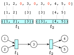
Figure 4.8: A way to convert a string to a Petri net, and vice-versa.

Quite soon though we realize that since strings are ordered, our substrings are not really specifying input and output of transitions – which are multisets – but source and target of their corresponding generating morphisms! That is, the procedure in Figure 4.8 can be used, without any change, also to pass around FSSMCs! It is clear then than even if we are visualizing the information in the string as a net, we are secretly dealing with its corresponding FSSMC. Computers simply like them more!

The way the Statebox language works, then, is the following: When a user draws a Petri net, its places and transitions are automatically indexed, and the structure is converted, under the hood, into its corresponding FSSMC. When transitions are fired, the user can specify which tokens a firing transition has to process (if there is any choice to be made), and the corresponding morphisms are composed in the FSSMC. Visualizing the state of an execution simply amounts to visualize the string diagram representing that history.

When a Petri net has to be morphed into another, a functor between their corresponding FSSMCs has to be specified. The user can just indicate which places and transitions have to be mapped to which places and transitions. This defines a morphism of Petri nets which is lifted to a functor between FSSMCs (in a non functorial way, as we said already) via some of the standard procedures explained in [12, Sec.4.3]. Alternatively, the user is able to define such procedures manually, de facto defining the functor between FSSMCs directly.

All in all, with this approach we use just FSSMCs, but Petri nets are used both to do model checking and prove properties about the code (which obviously the FSSMC preserves) or to provide enough basic information to allow the computer to infer the rest. As some researchers like to say, Petri nets are presentations of FSSMCs, meaning that they provide the bare minimum information to build and work with a given FSSMC. This is precisely the way we are using them.

4.8 Beyond standard Petri nets

Up to now, we considered normal Petri nets and categorically described their executions. But what happens if we change our notion of Petri net? A nice change to make would be, for instance, to allow the net to have negative tokens. If we represent a token as a black dot in a place, we can represent a negative token as red; we can moreover consider transitions that consume/produce negative tokens (Figure 4.9(a)). We call a net that allows for negative tokens an integer Petri net.

(a) Integer Petri net.

(b) Integer tokens.

(c) Before firing.

(d) After firing.

Figure 4.9:

If we start to explore this definition further, we see that very strange things can happen now. Since clearly a negative token and a positive one “annihilate”, exactly as $-1+1=0$, we can produce couples of tokens in any place, as in Figure 4.9(b). The consequence of this is that, as in Figures 4.9(c) and 4.9(d), now transitions can fire borrowing tokens from a place, and so they are always enabled!

Is there a use for this generalization? Most likely, yes. In fact, the study of executions of integer Petri nets is a genuine contribution of the Statebox team to academic research, that resulted in a paper [13], further generalized in [20]. What motivated us to investigate in this direction is that integer nets can be useful to model conflict resolution in concurrent behaviour. Consider, for instance, the net in Figure 4.10(a): We know that transitions $t_{1}$ and $t_{2}$ have to compete for the token in $p_{1}$ and, at least in the case of standard nets, they cannot both fire. Now suppose that there are two users, say $U_{1}$ and $U_{2}$, that can operate on the net, deciding which transition to fire. When a user takes a decision, it is broadcast to the other one, and the overall state of the net is updated. In a realistic scenario, though, broadcasting takes time (imagine, for instance, that our users have bad internet connections): User $U_{1}$ could decide to fire $t_{1}$ and user $U_{2}$ could decide to fire $t_{2}$ while the broadcast choice of $U_{1}$ has still to be received, putting the overall net into an illegal state (Figure 4.10(b)).

(a)

(b)

(c)

Figure 4.10:

In such a situation we need a way to re-establish consensus, that is, decide unambiguously in which legal state the net is. There are multiple ways to do this, but our main concern here is that the usual Petri net formalism does not have a way to represent illegal states, which is useful to attacking the problem mathematically. With integer Petri nets we are able to easily represent such a situation using negative tokens, as in Figure 4.10(c). Intuitively, we can say that a net is in an illegal state if the state contains a negative number of tokens in some place, and re-establishing consensus from an illegal state then amounts to getting back to one where the number of tokens in each place is non-negative. Clearly, the fact that any net can now fire just by borrowing positive tokens from its input places is consistent with the idea that, for whatever reason, every transition can put the net into an illegal state. There are, even, transitions like the one in Figure 4.9(a) that de facto “produce illegal states” out of thin air. This could be used, for instance, to represent a faulty component in our net architecture.

As we saw in this Chapter, the category of executions of a net carries much more information than the net itself, since we can track precisely the history of each token in the net. When it comes to integer nets, it makes sense to study this category to see if there are naïve ways to resolve an illegal situation, at least in some cases. The category of executions of an integer net looks very similar to what we already saw in Section 4.5, and we do not have to change much of what we already have. First, we need to add a new couple of bookkeeping morphisms in our formalism, along with identities and symmetries. These are depicted as a cup (Figure 4.11(a)) and a cap (Figure 4.11(b)), and represent the creation or annihilation of couples of negative and positive tokens in a place. These new morphisms have to satisfy the axioms in Figures 4.11(c) and 4.11(d) – these last couple of axioms are called yanking or snake equations [7], for obvious visual reasons. Strict symmetric monoidal categories that have cups and caps and respect such axioms are called strict compact closed categories [17].

(a) Cup.

(b) Cap.

(c) Axioms for cup and cap.

(d) Snake equations.

Figure 4.11: Additional structural morphisms and axioms for executions of integer nets.

As we did for standard nets, we need to define the concept of free strict compact closed category along with mappings that allow us to go from nets to categories, back and forth. This is not the right place to dive into the technicalities of this construction, for which we redirect the reader to [13]. What is really interesting, though, is to see how compact closed categories solve some of the problems regarding nets in illegal states, naïvely. For example, consider the situation in Figure 4.12: As before, imagine that a user $U_{1}$ fires transition $\tau$, while another user fires transition $\nu$ putting the net into an illegal state. We can represent this graphically in our category of executions introducing a cup that produces a pair of positive and negative tokens. At this point we apply a morphism corresponding to $\nu$ and carry the “positive part” produced by the cup to $Y$.

Now comes the interesting part: Suppose that some other user fires transition $\mu$. This transition produces a token in $X$ that effectively cancels the debt left in $X$ by the firing of $\nu$, reporting the net into an legal state. But this sequence of firings is still not acceptable, since the firing of $\nu$ could not have happened in the first place!

Nevertheless, the categorical model offers us a solution straight out of the box: When the token produced by $\mu$ lands in $X$, it annihilates the negative token left there. In the category of executions, this amounts to add a cap to our string diagram. But now the magic happens: We can straighten the string diagram using the snake equations obtaining the sequence of firings $\tau$, then $\mu$, then $\nu$.

Figure 4.12: Conflict resolution using integer Petri nets.

The right way to read the diagram in Figure 4.12 is as follows: The vertical lines divide different instants in time in the real world. If we were to attach a timestamp to each transition firing, we would actually observe that $\tau$ has been fired, then $\nu$ has been fired, and finally $\mu$ has been fired. On the contrary, the wire represents the causal flow of the network itself: It does not matter which transitions have been fired first in the real world, the flow represented by following the wire – namely $\tau$, then $\mu$, then $\nu$ – is the flow that does not break causality, allowing for a sequence of completely legal firings. The category of executions then offers naïve solutions to re-establishing consensus by reshuffling the order of transition firings, cancelling out any illegal state.

If we observe the net carefully, we notice that, actually, we still need to establish consensus on something: We presumed that user $U_{1}$ fired $\tau$ before user $U_{2}$, but obviously user $U_{2}$ is not of this opinion, otherwise he would not have fired $\nu$ in the first place.

This means that we need a way to establish which of the two users fired first, which is still a consensus problem. We argue, though, that this kind of consensus is much simpler to reach (for instance implementing a global clock) than having to reach consensus on an entire merging problem such as the one of re-establishing the causal order of transitions is. The category of executions for integer Petri nets takes care of this part of the problem for us, and needs only a very small amount of consensus to work properly.

All the details about this construction can be found in [13], where we proved results that are somewhat akin to the ones in Section 4.6. Namely, we arranged integer Petri nets in a category, called $\textbf{Petri}^{\mathbb{Z}}$. We did the same for categories of executions, obtaining a category of categories FSCCC. Finally, we produced a couple of mappings $\mathfrak{F}(-)$ and $\mathfrak{U}(-)$, which behave exactly like their counterparts in Section 4.6. Following the approach in [27], this time we were more interested in the mathematical results than in the implementation, so we massaged our categorical definitions a bit to be able to show an equivalence of categories.

The study of integer Petri nets is in its infancy, and many questions have yet to be answered. The “conflict resolution procedure” sketched in this Section, for instance, is only of theoretical interest at the moment and far away from an industry-strength implementation but we will keep pushing in this direction in the hope of obtaining something that can eventually become a useful feature to be used in our language.

It has to be noted that integer Petri nets also possess very nice characteristics when one tries to model transaction flows and money flows in general. This is relevant for a number of applications, among which are Blockchain-based techniques [22], for which it is commonplace to represent any kind of asset – even computations – by monetizing it [6], and the general characterization of economic phenomena in terms of process theories. This is the object of a broader research that the Statebox team is carrying out along with multiple partners, and which also involves open games [14], macroeconomics [34] and open systems [29].

4.9 Implementation

The FSSMCs formalism defines the very mathematical core of our way of representing net histories, hence it shouldn’t be surprising that implementing FSSMCs is a big chunk of our coding efforts.

Since we want formal guarantees that net histories evolve without errors, we are implementing FSSMCs in Idris. This has the desirable property that if we try to compose incompatible morphisms – e.g. we try to take the composition $f;g$ with $f:A\to B$ and $g:C\to D$, the result will be a typecheck error. In simple words, Idris’ typechecker won’t allow us to do any mathematically inconsistent operation. This way of implementing things is clearly very powerful, and brings our implementation as close to the actual mathematical theory as possible.

Unsurprisingly, we are using the idris-ct [32] library to define what a FSSMC is, but this is not a simple task: As we can see, Definition 4.4.4 builds a FSSMC by making use of equations that identify morphisms inside the category. From a mathematical point of view, we say that we are quotienting the morphisms. Unfortunately, Idris’ typesystem does not really like quotients, which are indeed quite difficult to deal with in type theory.

This prompted us to finding alternative, Idris-friendly ways to define FSSMCs. After really pushing the Idris compiler to its limits [24], we got a formal, complete definition of FSSMC.

Another implementation effort revolves around the idea of having the Idris core to insert symmetries in place for us during morphism composition. To see this, imagine to have a net history. As we know, we can represent this as a morphism in a FSSMC. Now assume that this history is a morphism $m:I\to B\otimes A$. In our interpretation, this means that we started with a net having no tokens, and fired transitions so that we now have a token in $B$ and a token in $A$. Suppose that now we fire a transition corresponding to the generating morphism $f:A\otimes B\to C$. We clearly can do this since $f$ is enabled in the net, but we quickly realize that we cannot take the composition $m;f$, since source and target of $f$ and $m$, respectively, do not match. To extend the history consistently, we need to do some bookkeeping, namely by inserting a symmetry in the composition, and taking $m;\sigma_{B,A};f$. The point is that in many situations – as for instance the one we sketched – there is only one way to define such symmetries. What we want, then, is a series of helpers and formal procedures to allow Idris to figure out these symmetries automatically whenever possible, to make the transition from Petri nets to FSSMCs as smooth as possible for the end user.

4.10 Why is this useful?

The answer to this question should be pretty clear: Executions allow us to track which transitions process which tokens, and to formalize the idea of “history of a net”. Being able to represent the causal relationships between firings precisely and reliably is fundamental to concatenate processes in a meaningful way, and categories of executions, serving exactly this purpose, will function as a bridge to consistently link nets, seen as abstract design tools for complex systems, to the actual implementation – we will start developing this point of view in Chapter 5. Note how leveraging this formal bridge is exactly what makes Statebox different from any other project based on Petri nets. Petri nets have, in fact, been used as design tools for software many times in the past, but the general modus operandi was as follows:

• The programmer would draft how the software about to be written was supposed to work in the abstract, using a Petri net. The properties of the net would be formally studied to ensure some pre-set performance standards;

• Afterwards, code would be produced, using the net implementation as a guide. This passage would be totally handmade and there would be no formal link between the net and the actual codebase. All things considered, the formal relationship between nets and code would amount to zero, and using nets to design it was not much different than sketching flow diagrams on a piece of paper: Helpful, but needing a lot of common sense to be implemented properly;

• As a consequence, it would happen that the software implementation could not properly reflect the net topology due to human error, and performing even small modifications in the net layout would result in huge code refactoring.

Category theory, on the other hand, completely automates all these steps giving us a neat way to represent net executions.

Chapter 5 Folds

In this Chapter we will reap what we sow up to now. Many of the concepts presented in the previous Chapters, purely theoretical on their own, will start displaying evident applicative potential when put together. Here we will sketch the actual plan to turn Petri nets and category theory into a useful software development toolkit.

We devoted Chapter 4 to the endeavor of building categories associated with Petri nets. We pointed out how the main reason to do this was to be able to describe the net behavior in a completely deterministic way, keeping track of the history of any token. In truth, we can do much more than this: If for each net $N$ we have a category $\mathfrak{F}(N)$, we can use our categorical intuition and do the most sensible thing when you have a category, namely mapping it to somewhere else by means of a functor.

5.1 Problem Overview

A perfectly legitimate question, at this stage, is: Why should we map executions to other categories? Note how, at the moment, both Petri nets and their executions cannot do much. We are able to draw a net and, as we said, we interpret its transitions as processes that, when firing, consume and produce resources, but where is this information stored? Clearly nowhere, at least for the moment. This interpretation exists only in our mind and is not backed up by any meaningful mathematics. Similarly, in defining executions, we said that we associate, to each transition, a family of morphisms representing the processes actually performed by the transition during firing. But again, this is an interpretation, since the actual definition of such processes is lacking in our category of executions. Recalling Definition 4.5.8, we obtain a morphism $t:\mathfrak{O}_{P_{N}}({{}^{\circ}}(t)_{N})\to\mathfrak{O}_{P_{N}}({(t)_{N}^{\circ}})$ for each transition $t$ by means of an inference rule, but that is pretty much it. Our processes lack any sort of actual specification.

(a) A net representing quicksort.

(b) Morphism associated to Figure 5.1(a).

Figure 5.1: Quicksort and its execution.

Example 5.1.1 (Quicksort).

Consider the net in Figure 5.1(a). We interpret the places as holding resources of type List[Int], that is, a token in a place represents a list of integers. Transition $t$ represents an application of the quicksort algorithm [16], that sorts the list. This information is clearly not captured by our net, which just describes how the transition turns one resource into another. Also our idea of tokens being of type List[Int] is overimposed, since the behavior of this data structure is not represented by the net (for instance, we cannot concatenate tokens or perform any sort of list operation on them). Similarly, in Figure 5.1(b) we represent the morphism associated to $t$ in its category of executions. Again, in this setting, $t$ is just “a box”, and the information describing its behavior (namely, quicksort) is nowhere to be found.

Example 5.1.2 (Is quicksort being done right?).

An obvious counterargument to the reasoning in Example 5.1.1 could be that the net in Figure 5.1(a) does not capture the meaning of the quicksort algorithm because it is not the right model for it: It is not that nets are bad at representing such a thing but that we have not used them properly. Up to some extent, this is actually the case, since we can definitely try to model sorting algorithms in a much more convincing way using nets. It is worth stressing that this is often not the right way of thinking about Petri nets. The application of a mathematical gadget in computer science should, nearly always, serve the purpose of stripping away complexity and making things easier, possibly without giving up formal correctness and consistency of our methods. Does it make sense, then, to spend time to define something that already has fully debugged and efficient implementations, spanning just a few lines of code? The answer is clearly no, since what we would get, at best, is something that needs a considerable amount of time and thought to get the level of performance found in existing solutions. Petri nets should make our life easier, and we would like to leverage already existing implementations of algorithms if we have them, as in the case of quicksort.

5.2 Mapping executions

What Example 5.1.1 entails could look like a huge downside: Our math is good for nothing, and our nets cannot do anything interesting without becoming really complicated. Luckily enough, this is not the case. What we obtained is, instead, far more valuable, and akin to what a logician would call the separation between syntax and semantics. We obtained a model of how our Petri nets behave without having to refer to any particular detail which complements the declarative functional approach we take in the implementation of our language. We can talk about quicksort, as in Example 5.1.1, without giving any specification of what quicksort does, aside of how it fits in the infrastructure we are designing, represented by the Petri net. The actual specification of quicksort (that is, its semantics) can be modeled separately in another category, and then be targeted appropriately by mapping the category of executions of the net into it. The fact that this mapping is functorial guarantees that syntax and semantics are being glued consistently together.

Example 5.2.1 (Design advantages).

The clear utility of this separation is that we can undertake our design efforts in stages. For instance, imagine that we are automating the infrastructure of an entire company. We first talk with people from various departments, asking them about their daily routines and needs. We then draft a Petri net describing how these processes interact with each other in real time, and since the Petri net formalism is completely graphical, people giving us this information even help us to visually debug it, pointing out where the diagram representing a process in their workflow is incorrect. After having done this, we apply tools to study reachability problems on the net, verifying that it has the properties that we desire (for instance absence of deadlocks or illegal states, recall Definition 2.5.3). If these requirements are not met, then we can reshape the net until we get what we want. At this point – and only at this point – we can start writing down the code (typically in a lower level language) for the programs associated to each transition, and the functorial mapping from the net execution to the actual code takes care of putting everything together.

Having intuitively described the essence of folds, let us try to fix the concept with a definition.

Definition 5.2.2 (Folds).

Given a Petri net $N$ and a symmetric monoidal category $\mathcal{S}$, a fold for $N$ is a symmetric lax monoidal functor (recall Definition 3.5.1) $\mathfrak{F}(N)\to\mathcal{S}$.

The reason we are choosing a Lax monoidal functor is because it is the weakest requirement we can think of. It is always a good practice to state something in the greatest level of generality possible, and strengthen the requirements only if needed.

Before we start digging into the real stuff, notice that there is an obvious fold that we can take:

Remark 5.2.3 (Trivial Fold).

The identity functor $\mathfrak{F}(N)\to\mathfrak{F}(N)$ is trivially symmetric lax monoidal, hence it generates a trivial fold for $N$. Note that this remark is what prompted for the notation $\mathfrak{F}(-)$ to define the category of executions of a net. Executions are, to some extent, the simplest fold possible, where the meaning we attach to any execution of the net is the execution itself.

To create more complicated instances of folds, we need to create semantic categories to which it makes sense to map executions. A good starting point is to recall Example 3.1.5, and use algorithms written in a functional programming language (Haskell, in our case) as semantics.

Definition 5.2.4 (Haskell, again).

The category Hask is defined as follows:

• Objects are data types. A data type is a way a computer uses to represent a certain kind of information. Common data types are Bool, consisting of the booleans True and False; Int, consisting of integer numbers, List[Int], consisting of finite lists of integer numbers, and many other;

• Morphisms are terminating haskell algorithms, that is, algorithms that take terms of some data type as inputs , apply a sequence of operations that at some point terminates, and output a term of some data type as a result.

The category Hask can be made into a symmetric monoidal category using the natural cartesian product structure that data types and morphisms admit (a product of types $A,B$ is just the type of couples $(a,b)$ where $a$ has type $A$ and $b$ has type $B$).

Remark* 5.2.5 (Is Hask a category?).

The reader with experience in the abstract theory of programming languages will have risen an eyebrow reading Example 5.2.4. In fact, the matter of defining the category Hask is quite a can of worms. In our case we are considering the strict symmetric monoidal category equivalent – via Remark 3.3.14 – to what is known in the functional programming folklore as the platonic Haskell category[15], where types do not have bottom values, valid morphisms are just terminating algorithms, algorithms are considered equal if they agree on all inputs and the use of seq is very limited. In general, the question of casting a category out of the Haskell programming language is still very debated, but we want to stress how this is not fundamental with respect to what we are going to do here. The point is that the fold from $\mathfrak{F}(N)$ to Hask is implementable, and offers a consistent way to map transitions into pieces of software.

Example 5.2.6 (The fold to Hask, in practice).

It is interesting to see how the mapping $\mathfrak{F}(N)\to\textbf{Hask}$ works in practice. Let us build a strict symmetric monoidal functor $F:\mathfrak{F}(N)\to\textbf{Hask}$: Each place in $P_{N}$ is also an object of $\mathfrak{F}(N)$, and as a consequence will be mapped by $F$ to a particular Haskell data type. We have complete freedom in defining this mapping as we please. The mapping on monoidal products of objects will then have to follow since we set, by definition, $F(u\otimes v)=(Fu,Fv)$.

Next, the bookkeeping morphisms. Identities on a object $u$ will be mapped to the algorithm $Fu\to Fu$ that takes any term of type $Fu$ in input and outputs the term itself without changing it. Symmetries $\sigma_{u,v}:u\otimes v\to v\otimes u$ will be mapped to the algorithm that takes tuples $(x,y)$ with $x$ of type $Fu$ and $y$ of type $Fv$ and outputs $(y,x)$.

For each transition $t\in T_{N}$ we get, from Definition 4.5.8, a morphism $t_{u,v}$ such that $\mathfrak{M}_{P_{N}}(u)={{}^{\circ}}(t)_{N}$ and $\mathfrak{M}_{P_{N}}(v)={(t)_{N}^{\circ}}$. Each one of these morphisms will be mapped to a Haskell algorithm $Ft_{u,v}:Fu\to Fv$.

Remark 5.2.7 (Strictness makes life easier).

Note that, in Example 5.2.6, requiring $F$ to be strict monoidal is what saved the situation, allowing us to define it only on places and transitions and leveraging strictness to extend it to all objects and morphisms. If we require $F$ to be just lax, then we have much more choice to define it, which is a good thing on the one hand, giving implementational freedom, but bad on the other, since we have to specify more things “manually” to make it work. The appropriate choice clearly depends on context.

Example 5.2.8 (Quicksort, continued).

We now turn our naïve interpretation of Example 5.1.1 to something formal. Call $N$ the net in Figure 5.1(a). We define the fold $\mathfrak{F}(N)\to\textbf{Hask}$ mapping $p_{1}$ and $p_{2}$ to List[Int], and $t$ to the code:

⬇

1 quicksort :: [Int] -> [Int]

2 quicksort [] = []

3 quicksort (p:xs) = (quicksort lesser) ++ [p] ++ (quicksort greater)

4 where

5 lesser = filter (< p) xs

6 greater = filter (>= p) xs

Finally, $t$ is now formally identified with quicksort!

Remark 5.2.9 (Terminating algorithms work better).

In Definition 5.2.4 we explicitly required morphisms of Hask to be terminating algorithms. It is worth to spend a few words on this: The interpretation of a fold is that transitions of a net get mapped to algorithms. Folds tell us which algorithm to run on which data when a transition fires. Clearly, in case the algorithm is not terminating, things break down: The transition in the net fires, but no tokens can be ever produced since the algorithm will hang forever. We get rapidly aware of how mapping transitions to algorithms that are not guaranteed to terminate is not, in general, good practice, since our formalism is no longer able to ensure consistency. This means that such “unsafe” mappings should be used only in very restricted contexts, when it is absolutely necessary, and in a very localized way, so that we are always able to keep track of which transitions in the net can exhibit a pathological behavior. Keeping the problem circumscribed is the easiest way to fix problems should they arise.

With respect to this, some functional programming languages such as Idris [4, 5] offer the useful functionality of a totality checker already embedded in their compiler. What this means is that, for a restricted class of algorithms, the compiler is able to tell us if our algorithm will terminate on every input. This feature is incredible in the context of Folds, since it will allow us to map transitions to code that we know to be well behaved.

5.3 Different folds, shared types

In reviewing the material covered in the last Section, we become aware that there is nothing special about using Hask as our semantics, and that in fact every functional programming language – or in general every language in which types can be defined – does, more or less, the job. One of the first things that comes to mind is: What happens if given a net $N$ we chose $\mathfrak{F}(M)$, for some other net $M$, to define the semantics of a fold? We are not requiring, here, for this functor to be generator-preserving, as we did in Chapter 4. The idea is that we could map a single transition of $N$ to an entire sequence of firings in $M$. This sort of “net inception” concept is very powerful, and backs up the intuition of transitions in a net triggering the execution of other nets as subprocesses, but needs far more work to be used properly.

What we can already do with the tools developed so far is sketching how different folds relate to each other:

Definition 5.3.1 (Morphisms of folds).

Given folds $F_{1}:\mathfrak{F}(N)\to\mathcal{S}_{1}$, $F_{2}:\mathfrak{F}(N)\to\mathcal{S}_{2}$, a morphism of folds is a symmetric lax monoidal functor $G:\mathcal{S}_{1}\to\mathcal{S}_{2}$ such that $F_{1};G=F_{2}$. Folds and their morphisms form a category.

Remark* 5.3.2.

The category of folds and their morphisms can be seen as the co-slice category of strict symmetric monoidal categories and symmetric lax monoidal functors over $\mathfrak{F}(N)$. $id_{\mathfrak{F}(N)}$ is clearly initial in this category.

Embracing the interpretation of semantics in terms of data types and algorithms, a morphism of folds can be seen as a “translation” from one programming language to another, that allows us to rewrite our mapping altogether. This is not very useful in practice: such translation exists very rarely since different programming languages have different properties.

What would be very useful, on the contrary, would be to have all the programming languages modeled in the same category. In fact, up to now, we are mapping executions into one programming language at a time, but this is not always what we would like to have. If our Petri nets represent a complex system, then transitions can represent processes radically different in nature, that would be better implemented in different programming languages, or, most likely, for which efficient implementations already exist in different languages.

With respect to this we want to be resourceful, and be able to use as much preexisting stuff as we can. Experienced programmers know, in fact, that one of the biggest barriers in the adoption of a new programming language is having to rewrite entire libraries from scratch: This is not only time-consuming, forcing developers to spend many hours of good work on just preparing the software instead of using it to solve the problems at hand, but also very inefficient, since rewriting complex code is a tedious process that needs a lot of further testing. In real-life applications, there is virtually no porting of industry-strength products that works out of the box, and in translating libraries from one language to another one is almost always guaranteed sub-optimal performance – both in terms of time/space efficiency and presence of bugs and errors – for a big portion of the development stage. The ideal semantic category we aim at, then, looks like this:

Definition 5.3.3 (Generalized semantics for folds).

Let $\mathcal{L}_{1},\dots,\mathcal{L}_{n}$ denote programming languages. We define a category having:

• As objects, data types of $\mathcal{L}_{1},\dots,\mathcal{L}_{n}$;

• As morphisms, terminating algorithms between data types in the languages $\mathcal{L}_{1},\dots,\mathcal{L}_{n}$.

Figure 5.2: A net showing how Definition 5.3.3 is pathological.

This definition is obviously pathological, and will never serve any real purpose. We can see it directly considering the net in Figure 5.2: Suppose that transition $t_{1}$ has to correspond to some very efficient algorithm we want to use, written in Haskell. On the other hand, the best choice for $t_{2}$ would be to map it to some code written in Elm [8, 9]. This implies that the place $p$ has to correspond to a data type that is shared by Haskell and Elm, which is basically impossible since different languages implement data types differently.

For the same reason, defining a symmetric monoidal structure on the category in Definition 5.3.3 is next to impossible, since we do not even know what it means to take tuples of data types defined using different specifications. Luckily enough, there is a solution to this problem, that relies precisely on defining a shared data type specification for different languages. It is clear that such shared data types will have to be somehow limited, since types have different capabilities in different languages (for the experienced readers, notice how Idris has dependent types while Haskell does not, so they cannot be part of our shared type structure). This is something to which the Statebox team is devoting a lot of work, and its specification, called Typedefs [31], is an open, ongoing project. Typedefs will make it easier to mix programming languages and will empower developers to use Petri nets to design their software without having to give up on the tools they already created, which is a very desirable feature.

5.4 Why is this useful?

The usefulness of folds is self-evident: They allow for neat compartmentalization of development stages and, by giving the programmer freedom to chose the semantic category that suits their needs best, ensure full backwards compatibility. With Typedefs, finally, this compatibility can be seamlessly extended across different languages, finally allowing for a consistent linking between different layers of a complex system. From the point of view of industry-strength coding, especially in fail-sensitive applications, such features are simply invaluable, and put Statebox into a unique status among the myriad of programming languages out there. As category theory is the glue of mathematics, Statebox is the glue of programming.

List of Symbols

Please note that some of the symbols we have used are overloaded (as for $\to$ to denote morphisms, functors and reachability). Their disambiguation depends on the context.

Sets

$S,T,\dots$	Generic set names, when usable
$\cup$	Set union
$\cap$	Set intersection
$\sqcup$	Set disjoint union
$\mathbb{N}$	Set of natural numbers
$\mathbb{Z}$	Set of integer numbers

Multisets

${X}^{\mathbb{N}}_{S}$	Finite multiset ${X}^{\mathbb{N}}_{S}:S\to\mathbb{N}$
${X}^{\mathbb{N}}$	Finite multiset ${X}^{\mathbb{N}}_{S}:S\to\mathbb{N}$, base implicit
${X}^{\mathbb{N}}_{S},{Y}^{\mathbb{N}}_{S},{Z}^{\mathbb{N}}_{S},\dots$	Generic finite multiset names, when usable
${X}^{\mathbb{N}},{Y}^{\mathbb{N}},{Z}^{\mathbb{N}},\dots$	Generic finite multiset names (base implicit), when usable
${S}^{\oplus}$	Set of finite multisets over $S$
$\subseteq$	Multiset inclusion
$\cup$	Multiset union
$-$	Multiset difference, defined when the second argument is included in the first
$\cdot$	Scalar multiplication of multisets
$\sqcup$	Disjoint union of multisets
$\emptyset_{S}$	Zero multiset over $S$
$\hookrightarrow$	Multiset injection
$\left|\quad\right|$	Cardinality of multisets
$g:{S}^{\oplus}\to{S^{\prime}}^{\oplus}$	Multiset homomorphism
$\bar{g}:{S}^{\oplus}\to{S^{\prime}}^{\oplus}$	Multiset homomorphism coming from function $g:S\to S^{\prime}$

Strings

$r,s,\dots$	Generic names for strings over $S$, when usable
$S^{\otimes}$	Set of strings of finite length over $S$
$\mathfrak{M}_{S}$	Multiplicity function from $S^{\otimes}$ to ${S}^{\oplus}$
$\mathfrak{O}_{S}$	Ordering function from ${S}^{\oplus}$ to $S^{\otimes}$

Petri nets

$N,M,L,\dots$	Generic net names, when usable
$p,q,\dots$	Generic place names, when usable
$t,u,v,\dots$	Generic transition names, when usable
$P_{N}$	Places of $N$
$T_{N}$	Transitions of $N$
${{}^{\circ}}(t)_{N}$	Input of transition $t$ of $N$
${(t)_{N}^{\circ}}$	Output of transition $t$ of $N$
${X}^{\mathbb{N}}$	Marking of a net
$N_{X}^{\mathbb{N}}$	Net $N$ along with its marking ${X}^{\mathbb{N}}$
$N_{X}^{\mathbb{N}}\xrightarrow{t}N_{Y}^{\mathbb{N}},\quad{X}^{\mathbb{N}}\xrightarrow{t}{Y}^{\mathbb{N}}$	Firing of $t$ in $N$, reachability of ${Y}^{\mathbb{N}}$ from ${X}^{\mathbb{N}}$
$\langle f,g\rangle$	Morphism of Petri nets

Category theory

Category names

FSCCC	Category of free compact closed categories and generator preserving functors
FSSMC	Category of free strict symmetric monoidal categories and generator preserving functors
$\textbf{FSSMC}_{G}$	Category of free strict symmetric monoidal categories and grounded generator preserving functors
Group	Category of groups and homomorphisms
Hask	Platonic Haskell category of datatypes and functions
hTop	Category of pointed topological spaces and homotopy classes of continuous functions
Petri	Category of Petri nets and morphisms between them
$\textbf{Petri}_{G}$	Category of Petri nets and grounded morphisms between them
$\textbf{Petri}^{\mathbb{Z}}$	Category of integer Petri nets and morphisms between them
Set	Category of sets and functions
Top	Category of topological spaces and continuous functions

Basic notions

$\mathcal{C}$	A category
$\mathcal{C},\mathcal{D},\mathcal{E},\dots$	Generic category names, when usable
$\operatorname{Obj}\,\mathcal{C}$	Objects of $\mathcal{C}$
$\operatorname{Hom}_{\,\mathcal{C}}$	Morphisms of $\mathcal{C}$
$A,B,C,\dots$	Generic object names, when usable
$f:A\to B,\quad A\xrightarrow{f}B$	Morphism from $A$ to $B$
$f,g,h,\dots$	Generic morphism names, when usable
$\operatorname{s}(f)$	Source (or domain) of morphism $f$
$\operatorname{t}(f)$	Target (or codomain) of morphism $f$
$f;g,\quad A\xrightarrow{f}B\xrightarrow{g}C$	Composition of $f$ and $g$
$f^{-1}$	Inverse of morphism $f$ (when it exists)
$F:\mathcal{C}\to\mathcal{D},\quad\mathcal{C}\xrightarrow{F}\mathcal{D}$	Functor from $\mathcal{C}$ to $\mathcal{D}$
$F,G,H,\dots$	Generic functor names, when usable
$FA$	Application of functor $F$ to object $A$
$Ff$	Application of functor $F$ to morphism $f$
$\mathfrak{D}$	A commutative diagram in some category
$\eta:F\to G$	Natural transformation between $F$ and $G$
$\eta,\tau,\dots$	Generic natural transformation names, when usable
$\eta_{A}$	Component of natural transformation $\eta$ on object $A$

Monoidal Categories

$(\mathcal{C},\otimes,I)$	Verbose notation for monoidal categories
$A\otimes B$	Monoidal product of objects $A$ and $B$
$f\otimes B$	Monoidal product of morphisms $f$ and $g$
$I$	Monoidal unit
$\alpha_{A,B,C}$	Associator component on $A,B,C$
$\lambda_{A}$	Left unitor component on $A$
$\rho_{A}$	Right unitor component on $A$
$\sigma_{A,B}$	Symmetry on $A,B$
$\epsilon:I^{\prime}\to FI$	Unit morphism for a lax monoidal functor
$\phi_{A,B}$	Composition component on $A,B$ for a lax monoidal functor

Limits, colimits

$\times$	Product (of sets, of categories, …)
$\pi_{1},\quad\pi_{2}$	Product projections
$\langle f,g\rangle$	Universal morphism of products applied to $f,g$
$\sqcup$	Coproduct (of sets, of categories, …); pushout (when subscripted, as in $\sqcup_{B}$)
$\iota_{1},\quad\iota_{2}$	Coproduct injections; pushout injections (when superscripted, as in $\iota_{1}^{B}$)
$[f,g]$	Universal morphism of coproducts applied to $f,g$; universal morphism of pushouts applied on $f,g$ (when subscripted, as in $[f,g]_{B}$)

Executions

FSSMC	Free strict symmetric monoidal category
$(\alpha,r,s)$	Generating morphism for a FSSMC
$\mathcal{S}_{S}$	Category of symmetries generated by a set $S$
$\mathfrak{F}(N)$	Category of executions of a net $N$
$\mathfrak{U}(-)$	Functor from FSSMC to Petri Functor from $\textbf{FSSMC}_{G}$ to $\textbf{Petri}_{G}$

Folds

$\mathcal{S}$	Generic name for categories serving as semantics
$\mathcal{L}$	Generic name to denote a programming language

Bibliography

- [1] John C. Baez and Jade Master “Open Petri Nets” In arXiv, 2018 arXiv: http://arxiv.org/abs/1808.05415
- [2] Paolo Baldan, Roberto Bruni and Ugo Montanari “Pre-Nets, Read Arcs and Unfolding: A Functorial Presentation” In Recent Trends in Algebraic Development Techniques 2755 Berlin, Heidelberg: Springer Berlin Heidelberg, 2003, pp. 145–164 DOI: 10.1007/978-3-540-40020-2_8
- [3] Francis Borceux “Handbook of Categorical Algebra: Volume 2, Categories and Structures” Cambridge: Cambridge University Press, 1994
- [4] Edwin Brady “Idris, a General-Purpose Dependently Typed Programming Language: Design and Implementation” In Journal of Functional Programming 23.05, 2013, pp. 552–593 DOI: 10.1017/S095679681300018X
- [5] Edwin Brady “Type-Driven Development With Idris” New York, NY: Manning Publications, 2017
- [6] Vitalik Buterin “A Next-Generation Smart Contract and Decentralized Application Platform” In Ethereum, 2014, pp. 1–36 URL: http://buyxpr.com/build/pdfs/EthereumWhitePaper.pdf
- [7] Bob Coecke and Aleks Kissinger “Picturing Quantum Processes: A First Course in Quantum Theory and Diagrammatic Reasoning” Cambridge: Cambridge University Press, 2017 DOI: 10.1017/9781316219317
- [8] Evan Czaplicki “Elm: Concurrent FRP for Functional GUIs” In Master thesis, Harvard University, 2012, pp. 55 URL: https://www.intranet.seas.harvard.edu/academics/undergraduate/computer-science/thesis/Czaplicki.pdf
- [9] Evan Czaplicki “Elm Homepage”, 2018 URL: http://elm-lang.org/
- [10] Samuel Eilenberg and Saunders MacLane “General Theory of Natural Equivalences” In Transactions of the American Mathematical Society 58, 1945, pp. 231–294 URL: http://www.ams.org/journals/tran/1945-058-00/S0002-9947-1945-0013131-6/S0002-9947-1945-0013131-6.pdf
- [11] Fabrizio Genovese “Behavioral Programming with Petri Nets a La Functional Way: Smart Contracts” In Statebox Blog, 2018 URL: https://blog.statebox.org/behavioral-programming-with-petri-nets-%C3%A0-la-functional-way-smart-contracts-96d801cef8cc
- [12] Fabrizio Genovese, Alex Gryzlov, Jelle Herold, Marco Perone, Erik Post and André Videla “Computational Petri Nets: Adjunctions Considered Harmful”, 2019 arXiv: http://arxiv.org/abs/1904.12974
- [13] Fabrizio Genovese and Jelle Herold “Executions in (Semi-)Integer Petri Nets Are Compact Closed Categories”, 2018 arXiv: http://arxiv.org/abs/1805.05988
- [14] Neil Ghani, Jules Hedges, Viktor Winschel and Philipp Zahn “Compositional Game Theory”, 2016 arXiv: http://arxiv.org/abs/1603.04641
- [15] HaskellWiki “The Category Hask” URL: https://wiki.haskell.org/Hask
- [16] C… Hoare “Algorithm 64: Quicksort” In Communications of the ACM 4.7, 1961, pp. 321 DOI: 10.1145/366622.366644
- [17] Gregory Maxwell Kelly and Maria L. Laplaza “Coherence for Compact Closed Categories” In Journal of Pure and Applied Algebra 19, 1980, pp. 193–213 DOI: 10.1016/0022-4049(80)90101-2
- [18] Saunders MacLane “Categories for the Working Mathematician” 5, Graduate Texts in Mathematics New York, NY: Springer New York, 1978 DOI: 10.1007/978-1-4757-4721-8
- [19] Saunders MacLane “Mathematics: Form and Function.” New York: Springer-Verlag, 1986
- [20] Jade Master “Generalized Petri Nets”, 2019 arXiv: http://arxiv.org/abs/1904.09091
- [21] José Meseguer and Ugo Montanari “Petri Nets Are Monoids” In Information and Computation 88.2, 1990, pp. 105–155 DOI: 10.1016/0890-5401(90)90013-8
- [22] Satoshi Nakamoto “Bitcoin: A Peer-to-Peer Electronic Cash System” In www.bitcoin.org, 2008, pp. 1–9 PMID: https://bitcoin.org/bitcoin.pdf
- [23] Mogens Nielsen “Models for Concurrency” In Mathematical Foundations of Computer Science 1991 520 Berlin, Heidelberg: Springer Berlin Heidelberg, 1991, pp. 43–46 DOI: 10.1007/3-540-54345-7_47
- [24] Marco Perone “Issue: Type Checker Hangs and Errors”, 2019 URL: https://github.com/idris-lang/Idris-dev/issues/4690
- [25] Carl Petri and Wolfgang Reisig “Petri Net” In Scholarpedia, 2008 URL: http://www.scholarpedia.org/article/Petri_net
- [26] Robert-Christoph Riemann “Modelling of Concurrent Systems: Structural and Semantical Methods in the High Level Petri Net Calculus” Munchen: Herbert Utz Verlag, 1999
- [27] Vladimiro Sassone “On the Category of Petri Net Computations” In TAPSOFT ’95: Theory and Practice of Software Development 915 Berlin, Heidelberg: Springer Berlin Heidelberg, 1995, pp. 334–348 DOI: 10.1007/3-540-59293-8_205
- [28] P. Selinger “A Survey of Graphical Languages for Monoidal Categories” In New Structures for Physics 813 Berlin, Heidelberg: Springer Berlin Heidelberg, 2010, pp. 289–355 DOI: 10.1007/978-3-642-12821-9_4
- [29] Pawel Sobociński “Representations of Petri Net Interactions” In CONCUR 2010 - Concurrency Theory 6269 Berlin, Heidelberg: Springer Berlin Heidelberg, 2010, pp. 554–568 DOI: 10.1007/978-3-642-15375-4_38
- [30] Statebox Team “Statebox Github Page”, 2017 URL: https://github.com/statebox/
- [31] Statebox Team “Typedefs Github Page”, 2018 URL: http://typedefs.com
- [32] Statebox Team “Idris-Ct Github Page”, 2019 URL: https://github.com/statebox/idris-ct
- [33] University of Torino “GreatSPN Github Page”, 2018 URL: https://github.com/greatspn/SOURCES
- [34] Viktor Winschel and Markus Kraetzig “Solving, Estimating, and Selecting Nonlinear Dynamic Models Without the Curse of Dimensionality” In Econometrica 78.2, 2010, pp. 803–821 DOI: 10.3982/ECTA6297