A practical way to regularize unfolding of sharply varying spectra with low data statistics

Abstract

Unfolding is a well-established tool in particle physics. However, a naive application of the standard regularization techniques to unfold the momentum spectrum of protons ejected in the process of negative muon nuclear capture led to a result exhibiting unphysical artifacts. A finite data sample limited the range in which unfolding can be performed, thus introducing a cutoff. A sharply falling “true” distribution led to low data statistics near the cutoff, which exacerbated the regularization bias and produced an unphysical spike in the resulting spectrum. An improved approach has been developed to address these issues and is illustrated using a toy model. The approach uses full Poisson likelihood of data, and produces a continuous, physically plausible, unfolded distribution. The new technique has a broad applicability since spectra with similar features, such as sharply falling spectra, are common.

1 Introduction

The procedure of extracting a “truth level” physics distribution that can be directly compared to a theoretical model from measured quantities affected by finite detector resolution is called unfolding Cowan1998 . The mathematical problem of unfolding is known to be ill-posed: truth level spectra that are significantly different from each other can map into detector distributions that have only infinitesimally small differences Blobel:1984ku ; Cowan1998 ; Cowan:2002in ; Prosper:2011zz . The best possible unbiased solution of an unfolding problem would have an unacceptably large variance Cowan1998 . It has been shown that approximate solutions to unfolding problems can be obtained by using a regularization procedure Tikhonov1963a ; Tikhonov1963b ; Phillips1962 , which reduces the variance of the result at the price of introducing a bias. Implementations of unfolding algorithms for particle physics applications, such as RUN/TRUEE Milke:2012ve and TUnfold Schmitt:2012kp exist. However they are based on the Gaussian approximation of the log-likelihood function, and regularized unfolding using the complete Poisson likelihood is still listed in the “ideas” section in this year’s conference talk Schmitt:phystat2019 .

The current work was performed in the context of measuring momentum spectrum of charged particles emitted in the process of negative muon capture on atomic nuclei at rest twist-mucapture . The median number of data entries in non-empty bins of a reconstructed 2-dimensional distribution was about 10, necessitating the use of Poisson likelihood in the analysis. The spectrum varied by more than an order of magnitude in the unfolding region. A straightforward application of standard regularization techniques, introduced in section 2 to a toy model, defined in section 3, yielded unfolded spectra with undesirable artifacts, as described in section 4 below. Section 5 presents modifications to the unfolding procedure that allowed us extract the result without unphysical features. Section 6 discusses the choice of regularization strength, and 7 summarizes the findings.

2 Regularized unfolding

The formulation of the unfolding problem involves an experimental observable $x$, truth level variable $y$ with unknown distribution $f(y)$, which we would like to determine, and detector response $R$. Both experimental observables and truth level variables are in general multidimensional. For example, in the capture measurement twist-mucapture truth level information comprises particle species and its true momentum, while experimental observables include measured track momentum and its range in the detector.

We consider the case when the experimental spectrum is binned. Detector response $R_{i}(y)$ is the expectation value of the number of reconstructed events in bin $i$ given a true event occurring at $y$. It describes all the detector effects: acceptance, efficiency, and resolution—but is independent of the physics spectrum that is being measured. Detector response is usually determined from a Monte-Carlo simulation, which forces a discretization in the $y$ space: $\int{R_{i}(y)f(y)\,dy}\longrightarrow\sum_{j}R_{ij}f_{j}$ where $f_{i}$ is the integral of $f(y)$ over bin $j$. The bin size in the $y$ space has to be much smaller than the experimental resolution in order for the simulation-derived $R_{ij}$ to be independent of the particular truth level spectrum shape used in the simulation. Small bin size in $y$ leads to a large number of unknowns $f_{j}$. This large number of unknowns is purely technical and is not related to the number of effective degrees of freedom of the problem, which scales with the size of the dataset Panaretos:2011bxp . However it can make non-linear numerical minimization not feasible. To reduce the number of degrees of freedom to a physically appropriate value one can approximate the unknown functions with splines Blobel:1984ku , as is illustrated later in this paper.

The expected number of data events in bin $i$, $\mu_{i}$, can be written as

$$\mu_{i}=N_{\text{true}}\sum_{j}R_{ij}f_{j}+b_{i}$$ (1)

where $N_{\text{true}}$ is the true number of events of interest in the dataset, and $b_{i}$ is the background contribution. A maximum likelihood estimator for $f_{j}$ is formed by minimizing

$$-\log{\mathcal{L}}(d|\mu\{f\})=-\sum_{i}(d_{i}\log\mu_{i}-\mu_{i})$$ (2)

where $d_{i}$ is the observed number of data events in bin $i$. However the unfolding problem is ill-posed and must be regularized to obtain a useful solution. Regularized unfolding can be performed by minimizing a combination of the log likelihood of data and a regularization functional $S\{f\}$ Tikhonov1963a ; Tikhonov1963b ; Phillips1962 .

$${\mathcal{F}}=-\log{\mathcal{L}}(d|\mu\{f\})-\alpha S\{f\}$$ (3)

where $\alpha$ is the regularization parameter.

A widely used Tikhonov Cowan1998 ; Tikhonov1963a ; Tikhonov1963b ; Phillips1962 regularization imposes a “smoothness” requirement on the spectrum by penalizing the second derivative of the solution. It therefore biases the result towards a linear function. Another well established regularization, the maximum entropy (or “MaxEnt”) approach Cowan1998 , is based on the entropy of a probability distribution Shannon:1948zz :

$$S_{\text{MaxEnt}}=-\sum_{j}q_{j}\ln(q_{j}),\qquad q_{j}\equiv f_{j}/\sum_{k}f_{k}$$ (4)

It biases unfolding result towards a constant.

Unfolding with Tikhonov regularization can be implemented in a computationally efficient way when $\chi^{2}$ minimization is used. However this advantage is lost when Poisson likelihood is needed. On the other hand, MaxEnt guarantees that the unfolded spectrum is positive, as is required for a particle emission spectrum, whereas Tikhonov with a large regularization strength $\alpha$ pulls the solution towards a straight line, which can cause some of $f_{j}$ to be negative. The present work uses the MaxEnt regularization term.

3 Toy model

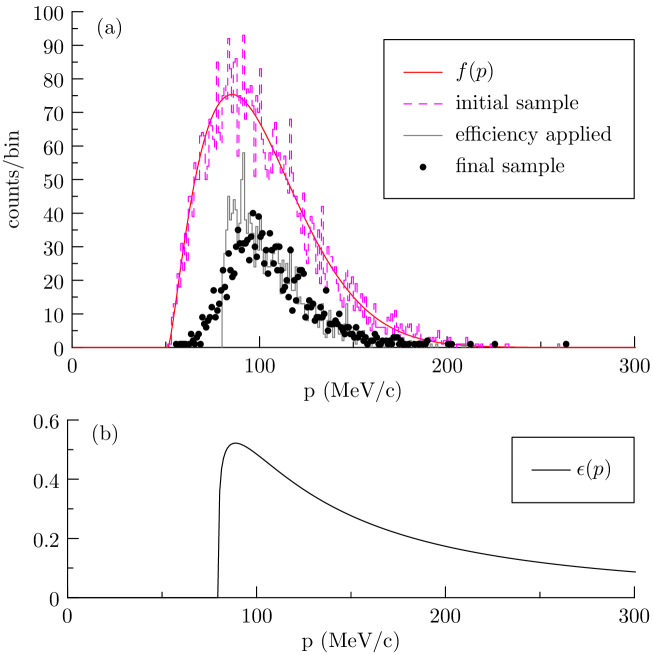
Figure 1: (a) Toy model momentum spectrum $f(p)$ and a random distribution of events drawn from it (initial sample), the distribution modified by detector acceptance times efficiency, and the final distribution after smearing. See text for more details. (b) Toy model detector acceptance times efficiency vs momentum.

Unfolding issues will be illustrated using a one-dimensional toy model that demonstrates some features first observed in the real life application of the technique. The model is based on the spectrum of protons ejected in the process of negative muon nuclear capture. The spectrum is known to follow an exponential distribution in kinetic energy for large proton energies, and to have a low energy threshold due to the Coulomb barrier Measday:2001yr . We use the empirical functional shape and parameters proposed in Hungerford:1999 , and convert the distribution from kinetic energy to momentum space:

$$f(p)=C\frac{p}{\sqrt{p^{2}+m^{2}}}\times\left(1-\frac{1.40\text{~{}MeV}}{T(p)}\right)^{1.3279}\times\exp\left\{-\frac{T(p)}{3.1\text{~{}MeV}}\right\}$$ (5)

where $m=938.27\text{~{}MeV}/c^{2}$ is the proton mass, $C$ is a normalization constant, and $T(p)=\sqrt{p^{2}+m^{2}}-m$ is the kinetic energy of the proton. The distribution is shown in Fig. 1(a). Detector efficiency times acceptance is modeled as

$$\epsilon(p)=\begin{cases}0,&p<=p_{0}\\ \left(\displaystyle\frac{p}{p_{0}}-1\right)^{0.2}\times\left(\displaystyle\frac{p}{p_{0}}\right)^{2},&p>p_{0}\end{cases}$$ (6)

with $p_{0}=80\text{~{}MeV}/\text{c}$, illustrated in Fig. 1(b). The momentum resolution of the toy detector model as a Gaussian with $\sigma=10\text{~{}MeV}/\text{c}$.

A sample of 5000 momentum values was drawn from the $f(p)$ distribution (the “initial sample” in Fig. 1(a)). Some of the “events” were randomly dropped following the $\epsilon(p)$ curve, then each remaining momentum smeared with the Gaussian resolution to form the “final sample” of 1569 events used for the unfolding tests below. The response matrix for the tests was computed analytically and contains no statistical fluctuations, corresponding to the limit of infinite MC statistics. The toy model contains no background.

4 Example of application

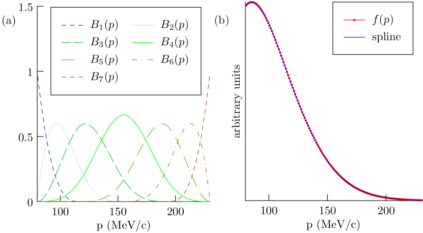
Figure 2: (a) A set of B-splines. (b) $f(p)$ approximated by a linear combination of the splines.

To implement the approach outlined in section 2 we need to define an unfolding interval and select a set of splines on that interval to approximate the distribution being unfolded. Cubic $B$-splines Boor1978b provide a convenient basis for modeling smooth continuous physics distributions. Figure 2(a) shows a set of cubic $B$-splines obtained by placing 3 internal knots that split the interval $80\text{~{}MeV}/\text{c}<p<230\text{~{}MeV}/\text{c}$ into 4 equal parts, and locating all other necessary knots at the end points Boor1978b . Figure 2(b) illustrates how a linear combination of these splines can approximate the function $f(p)$ from Eq. 5:

$$f(p)\approx\sum w_{i}B_{i}(p).$$ (7)

where $B_{i}(p)$ are the basis splines, and the $w_{i}$ are coefficients.

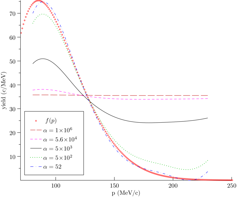
Figure 3: Unfolding results.

The unfolding is performed by minimizing Eq. 3 with respect to $w_{i}$ for a fixed value of $\alpha$. The choice of a starting point is critical for the success of a nonlinear multi-dimensional minimization. Our implementation starts with $f_{j}=\text{const}$ being an exact minimum of (3) for $\alpha\to\infty$, and minimizes the target functional for a large finite value of $\alpha$. Then $\log\alpha$ is reduced by a small amount, and the minimization is re-run by using the previous minimum as the starting point. As $\log\alpha$ is further reduced, each new minimization starts at a point that is linearly interpolated from the two previously found mimima. The process is repeated until the desired value of regularization strength is reached.

Figure 3 shows results for several settings of regularization strength $\alpha$. As it is reduced, the solution changes from an almost constant function for $\alpha=10^{6}$, dominated by the entropy term $S\{f\}$, to curves that are influenced by the likelihood of “data” $\log{\mathcal{L}}(d|\mu\{f\})$. The $f(p)$ spectrum used to produce the toy MC sample is also shown figure 3. One can see that $\alpha=5\times 10^{2}$ is still too large, and the corresponding curve does not reach $f(p)$ in both its peak and tail regions. On the other hand, it already develops a unphysical rising behavior at the end of the unfolding range. Using a lower value $\alpha=52$ produces a spectrum that oscillates about the ideal result and has a pronounced rise at the end of the range.

The toy model example illustrates a typical behavior observed in a real life applications of the unfolding technique. In some cases the procedure does not yield a satisfactory result for any value of $\alpha$. The result spikes at the end, and if one moves the upper boundary of the unfolding interval the spike moves with it. There are two effects that “pull up” the distribution at the end of the unfolding region: the $S\{f\}$ regularization term, and the effect of “overflows” (i.e. reconstructed events that originated outside of the unfolding interval). The regularization term bias is exacerbated due to the fact that a constant is not a good approximation for the rapidly falling true distribution function. A generalization of the MaxEnt approach, cross entropy regularization Schmelling:1993cd ; Cowan1998 , allows to bias to an arbitrary reference distribution instead of a constant. The distortion due to overflow events can be addressed by treating the part of the signal distribution outside of the unfolding region as a fixed shape background, as is done in e.g. Schmitt:2012kp . In that approach the model of the signal distribution is not continuous, because the resulting distribution in the unfolding region does not generally match the a priori “background” distribution at the interval ends. Instead of trying to guess the steepness of the “true” distribution for the cross entropy and overflow background priors, we suggest to fit it from data, as is detailed below.

5 An improved technique

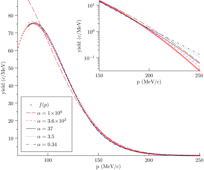
Figure 4: Results for the improved technique.

The main ideas to improve on the results of the previous section are:

• Inside the unfolding region, bias towards a physically motivated function instead of a constant, with parameters of the function included in the fit. For the spectrum of protons from muon capture example an exponential in kinetic energy was chosen, because the spectrum is know to approach this shape at high energies. Note that the true distribution in the toy model (Eq. 5) is not a simple exponential, however an exponential is a much better approximation for it in the unfolding interval than a constant.

• Include the “overflow” region in the minimization, and fit not just the normalization but also the exponential slope in that region.

• Require that the distribution is continuous and has two continuous derivatives. This requirement connects the unfolded distribution to the overflow tail in a way that prevents the unphysical spike at the boundary.

Specifically, we represent

$$f(p)=A\frac{p}{\sqrt{p^{2}+m^{2}}}\exp\{-\gamma T(p)\}\times\begin{cases}1+\phi(p)&p_{\text{min}}<p\leq p_{\text{max}}\\ 1&p_{\text{max}}<p\end{cases}$$ (8)

where $p_{\text{min}}$ and $p_{\text{max}}$ determine the limit of the unfolding region, $m$ is the mass of the particle and $T(p)$ its kinetic energy, $A$ and $\gamma$ are parameters pertaining to the exponential behavior of the spectrum, and $\phi(p)$ is an arbitrary function to be determined from the unfolding. The regularization term has the form (4) but now acts on $1+\phi$ instead of $f$:

$${S}_{\text{MaxEnt}}=-\sum_{j}\tilde{q}_{j}\ln(\tilde{q}_{j}),\qquad\tilde{q}_{j}\equiv(1+\phi_{j})/\sum_{k}(1+\phi_{k})$$ (9)

The function $\phi(p)$ is approximated by a linear combinations of cubic basis splines $B_{l}$ Boor1978b

$$\phi(p)=\sum_{l}^{n}w_{l}B_{l}(p),\qquad p_{\text{min}}<p\leq p_{\text{max}}$$ (10)

Here $w_{l}$ are the spline coefficients determined from the unfolding process. We require that the resulting spectrum has a continuous second derivative, leading to $\phi(p_{\text{max}})=\phi^{\prime}(p_{\text{max}})=\phi^{\prime\prime}(p_{\text{max}})=0$, which is provided by having a single-fold spline knot at the endpoint $p_{\text{max}}$. There are no continuity constraints at $p_{\text{min}}$, therefore a 4-fold knot should be used at that point to support the most general cubic spline shape.

To illustrate the modified technique, we use the same unfolding interval $80\text{~{}MeV}/\text{c}<p<230\text{~{}MeV}/\text{c}$ as in section 4 and the same set of internal knots. The resulting splines are $B_{1}$ to $B_{4}$ shown in Fig. 2. Splines $B_{5}$ to $B_{7}$ would violate the continuity condition and must not be included. Like before, we start with the maximally regularized solution and reduce $\log\alpha$ in small steps. The resulting curves for several values of $\alpha$ are shown in Fig. 4. Note that the starting solution ($\alpha=1\times 10^{6}$) is now close to an exponential, not a constant, and that some of the resulting curves closely follow the original $f(p)$ from Eq. 5.

6 Choice of the regularization strength

Figure 5: L-curve for the improved technique.

The regularization strength $\alpha$ in Eq. (3) should be chosen to provide an optimal balance between the variance and the bias of the result. The L-curve Hansen:1992 ; Hansen:1993 provides a way to visualize a transition from strongly biased, regularization term dominated solutions for large $\alpha$, to noise dominated ones. For a given $\alpha$ the minimization of ${\mathcal{F}}$ in Eq. (3) yields particular values of $\log{\mathcal{L}}$ and $S$. Our code minimized a binned likelihood ratio, so this is what we will use below instead of the “bare” $\log\mathcal{L}$. Following Hansen:1993 , we define parametric functions $\rho(\alpha)=-\log\left({\mathcal{L}}(d|\mu)/{\mathcal{L}}(d|d)\right)$ and $\eta(\alpha)=S$, and consider the curve $-\log\eta(\alpha)$ vs $\log\rho(\alpha)$. The choice of signs in the definition of the $\eta$ term provides the conventional orientation of the “L”. A plot of the curve is shown in Fig. 5. As $\alpha$ is initially reduced from $\alpha=1\times 10^{6}$, the curve is almost horizontal, with quality of fit to data improving while not significantly affecting the regularization term. For small $\alpha$ the regularization penalty grows sharply without much improvement in the data fit. The optimal value of $\alpha$ lies in the transition region, and can be defined as the point of the maximum curvature on the L-curve Hansen:1993 .

In our example, the maximum curvature point is at $\alpha=37$. The corresponding unfolded spectrum is shown as the solid line in Fig. 4. It is indeed a reasonable fit: the curves for smaller $\alpha$ are farther away from the correct solution for $p>200\text{~{}MeV}/\text{c}$ and $150<p<170\text{~{}MeV}/\text{c}$, while the curve for a larger $\alpha=3.6\times 10^{2}$ deviates more in the peak region $p\approx 80\text{~{}MeV}/\text{c}$.

7 Conclusion

The proposed method combines unfolding to an arbitrary function shape in a phase space region with sufficient data statistics and a parametric fit in the low statistics tail. The whole distribution is required to be twice continuously differentiable, which guarantees a physically reasonable behavior of the result. Factoring out the exponential part of a sharply varying spectrum and applying the regularization to just the deviation from the pure exponent reduces the bias. The use of the L-curve approach for finding the optimal regularization strength has been demonstrated for Poisson likelihood fit to data with the MaxEnt regularization term.

- (1) G. Cowan, Statistical Data Analysis. Clarendon Press, Oxford, New York, 1998.
- (2) V. Blobel, Unfolding Methods in High-energy Physics Experiments, in Proceedings, CERN School of Computing: Aiguablava, Spain, September 9-22 1984, 1984.
- (3) G. Cowan, A survey of unfolding methods for particle physics, Conf. Proc. C0203181 (2002) 248.
- (4) H. B. Prosper and L. Lyons, eds., Proceedings, PHYSTAT 2011 Workshop on Statistical Issues Related to Discovery Claims in Search Experiments and Unfolding, CERN,Geneva, Switzerland 17-20 January 2011, (Geneva), CERN, CERN, 2011. 10.5170/CERN-2011-006.
- (5) A. N. Tikhonov, Solution of incorrectly formulated problems and the regularization method, Soviet Mathematics Dokl. 4 (1963) 1035–1038.
- (6) A. N. Tikhonov, Regularization of ill-posed problems, Soviet Mathematics Dokl. 4 (1963) 1624.
- (7) D. L. Phillips, A technique for the numerical solution of certain integral equations of the first kind, J. Assoc. Comput. Mach. 9 (1962) 84.
- (8) N. Milke, M. Doert, S. Klepser, D. Mazin, V. Blobel and W. Rhode, Solving inverse problems with the unfolding program TRUEE: Examples in astroparticle physics, Nucl. Instrum. Meth. A697 (2013) 133 [1209.3218].
- (9) S. Schmitt, TUnfold: an algorithm for correcting migration effects in high energy physics, JINST 7 (2012) T10003 [1205.6201].
- (10) S. Schmitt, The collider experience with unfolding, in PHYSTAT-nu 2019 workshop, January 22–25, CERN, 2019, https://indico.cern.ch/event/735431/contributions/3137825.
- (11) TWIST Collaboration, “Charged particle spectra from capture on aluminum.” (in preparation).
- (12) V. M. Panaretos, A Statistician’s View on Deconvolution and Unfolding, in Proceedings, PHYSTAT 2011 Workshop on Statistical Issues Related to Discovery Claims in Search Experiments and Unfolding, CERN,Geneva, Switzerland 17-20 January 2011, (Geneva), pp. 229–239, CERN, CERN, 2011, DOI.
- (13) C. E. Shannon, A mathematical theory of communication, Bell Syst. Tech. J. 27 (1948) 379.
- (14) D. Measday, The nuclear physics of muon capture, Phys.Rept. 354 (2001) 243.
- (15) E. V. Hungerford, Comment on proton emission after muon capture, Tech. Rep. 034, MECO Collaboration, available as arXiv:1803.08403, 1999.
- (16) C. de Boor, A Practical Guide to Splines. Springer Verlag, New York, 1978.
- (17) M. Schmelling, The Method of reduced cross entropy: A General approach to unfold probability distributions, Nucl. Instrum. Meth. A340 (1994) 400.
- (18) P. C. Hansen, Analysis of discrete ill-posed problems by means of the L-curve, SIAM Review 34 (1992) 561.
- (19) P. C. Hansen and D. F. O’Leary, The use of the L-curve in the regularization of discrete ill-posed problems, SIAM J. Sci. Comput. 14 (1993) 1487.
- (20) M. Galassi et al., “GNU Scientific Library Reference Manual (3rd Ed.) ISBN 0954612078.” http://www.gnu.org/software/gsl/.
- (21) A. Hammerlindl, J. Bowman and T. Prince, “Asymptote: the vector graphics language.” http://asymptote.sourceforge.net.