Probing slow earthquakes with deep learning

Abstract

Slow earthquakes may trigger failure on neighboring locked faults that are stressed enough to break, and slow slip patterns may evolve before a nearby great earthquake. However, even in the clearest cases such as Cascadia, slow earthquakes and associated tremor have only been observed in intermittent and discrete bursts. By training a convolutional neural network to detect known tremor on a single seismic station in Cascadia, we isolate and identify tremor and slip preceding and following known larger slow events. The deep neural network can be used for the detection of quasi-continuous tremor, providing a proxy that quantifies the slow slip rate. Furthermore, the model trained in Cascadia recognizes tremor in other subduction zones and also along the San Andreas Fault at Parkfield, suggesting a universality of waveform characteristics and source processes, as posited from experiments and theory.

Geophysical Research Letters

Los Alamos National Laboratory, Geophysics Group, Los Alamos, New Mexico, USA Laboratoire de Géologie, Département de Géosciences, École Normale Supérieure, PSL Research University, CNRS UMR 8538, Paris, France Department of Geophysics, Stanford University, Stanford, California, USA

B. Rouet-Leducbertrandrl@lanl.gov

Deep learning models can recognize tremor on a single seismic station

New detections of weak tremor increase weeks to months before slow earthquakes

A model trained to detect tremor in Cascadia can detect known tremor from Japan and California with no further training

Plain Language Summary

Slow earthquakes cyclically load fault zones and have been observed preceding major earthquakes on continental faults as well as subduction zones. Slow earthquakes and associated tremor are common to most subduction zones, taking place down dip from the neighboring locked zone where megathrust earthquakes occur. In the clearest cases, tremor is observed in discrete bursts that are identified from multiple seismic stations. By training a convolutional neural network to recognize known tremor on a single station in Cascadia, we detect weak tremor preceding and following known larger slow earthquakes, the detection rate of these weak tremors approximates the slow slip rate at all times, and the same model is able to recognize tremor from different tectonic environments with no further training.

Introduction

In many subduction zones where megaquakes occur, slow earthquakes take place deep on the subduction interface, perturbing the stress environment of the neighboring and shallower locked zone, and potentially influencing the occurrence of large megathrust earthquakes[Ito . (2013), Vidale  Houston (2012)]. As a result, the relation between slow earthquakes and the locked zone is a topic of intense interest. Non-volcanic tremor, the noise-like seismic signature of slow earthquakes emanating from the subduction zone, was discovered relatively recently [Obara (2002), Rogers  Dragert (2003)]. Tremor is identified and located by analyzing the phase correlations of seismic signal envelopes recorded at multiple seismometers [Obara (2002), Obara  Kato (2016)]. Tremor is frequently used as a qualitative proxy for slow slip [Vidale  Houston (2012), Ide (2012)], including in situations where GPS shows no displacement, presumably because deformation at the surface is too small to record [Frank (2016)].

In an effort to characterize tremor from seismic noise and probe the relationship between tremor and slip (Fig. 1), we use a method based on convolutional neural networks (CNNs), a type of deep learning algorithm. CNNs are at the core of recent dramatic advances in computer vision, natural language processing and recommender systems [LeCun . (2015)]. The use of CNNs to recognize tremor can be viewed as a deep learning extension of template matching methods [Gibbons  Ringdal (2006), Frank  Shapiro (2014)], where the deep learning model automatically determines which time-frequency patterns to use, effectively learning something akin to a set of templates that are more general representations of tremor than hand-crafted templates. Tasked with recognizing tremor from portions of single station seismic data, the convolutional layers learn to represent inputs as a collection of simpler characteristic features. These features are then fed to the dense layers of the CNN, that learns to classify whether a portion of seismic data contains tremor or not based on this transformed representation.

Results

Deep learning tremor

The CNN model is trained on seismic data from the Canadian National Seismograph Network (CNSN) [Canadian National Seismograph Network (1989)]. Figure 2A shows the area analyzed: Vancouver Island on the North American Plate and the subducting Juan de Fuca plate, with a schematic of the locked and slowly slipping portions of the downgoing slab. Our ground truth for the initial training of the neural network is a tremor catalog from the Pacific Northwest Seismic Network (PNSN). The catalog was constructed using Wech’s tremor identification method (multi-station, based upon 5 minute envelope correlation) [Wech  Creager (2008)] from the southern portion of Vancouver Island between October 2009 to July 2017. We build our database from 5 minute portions of single station seismograms. For every tremor event in the PNSN catalog, we record the corresponding 5 minute single station waveform, and label it as containing tremor. For the non-tremor examples we randomly sample the seismic data on days where no tremor was identified in the PNSN catalog. This results in about 47,500 time windows of 5 minute single station waveforms labeled as containing tremor, and 47,500 windows of 5 minute single station waveforms labeled as not containing tremor. In order to leverage the ability of CNNs to extract information from images, instead of feeding raw waveforms to the CNN, we first compute the short-time Fourier transform (STFT) of the 5 minute portions of data (Fig. 1B). The original 5 minute waveforms containing 12’000 data points are converted into spectrograms over the 5 minute interval. These steps result in our database of 95,000 labeled ‘tremor’ and ‘absence of tremor’ examples (Fig. 1D,E).

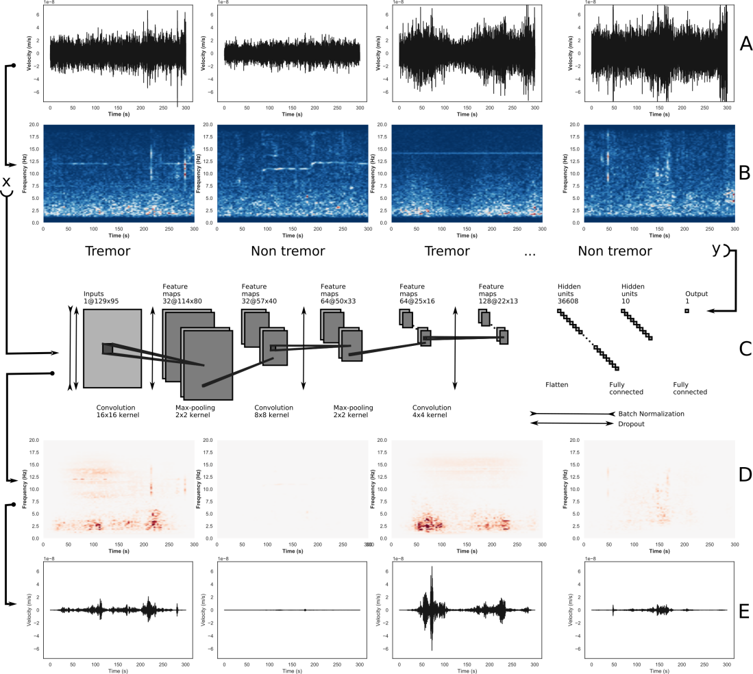
Figure 1: Deep learning tremor. (A) 5-minute duration, single station (NLLB) seismic signals. (B) Short-time Fourier transform of the waveforms that are fed as input to the convolutional neural network. (C) Schematic of the CNN and its architecture. The convolutional layers learn representations (features) of tremor while the last dense layers determine detection/no detection of tremor based on the presence of these features in a spectrogram. The model is trained on spectrograms labeled using the PNSN catalog of tremor from southern Vancouver Island from 2009 to 2015. (D) Interpretation of the CNN using Taylor decomposition[Montavon . (2017)], showing in red which parts of the spectrograms were recognized as characteristic of tremor. (E) Reconstruction of the waveforms from only the portions of the spectrograms recognized as tremor according to the CNN and its interpretation.

We split our database of 95’000 time (frequency) windows into two contiguous portions for training and testing: the first 80$\%$ for training and the last 20$\%$ for validation (10$\%$) and testing (10$\%$). In other words, all the examples from the end of 2009 to the end of 2015 are used to train the model, the examples from the end of 2015 to the end of 2016 are used for validation, and the examples from the end of 2016 to the end of 2017 are used to test and assess the model. The split of training data into contiguous pieces is of paramount importance for time series in general, and for this problem in particular. For instance, applying a random train/test split would assign pieces of any tremor burst longer than a few minutes to both the training and the testing set, making the problem dramatically easier – the CNN would only have to memorize the examples it sees in training.

The architecture of the CNN consists of three convolutional layers and one fully connected hidden layer (see Fig 1 and Methods for details). At the end of the training procedure (Fig. S1) the model is fixed and applied to the testing set (the last year of data never analyzed before), to assess how well it generalizes to new examples of tremor.

The CNN outputs an empirical probability that a portion of waveform transformed into the time-frequency domain contains tremor. The performance of the model, measured through the ROC-AUC metric, is shown in Fig. 2. The ROC curve is generated by plotting true positive rate of the model on the y-axis versus the false positive rate on the x-axis at progressively larger threshold settings. The further the curve is from the diagonal line and closer to the upper left corner, the better the model is at discriminating between positives and negatives. Lowering the classification threshold classifies more items as positive, thus increasing both false positives and true positives. For our purposes, true positives are catalogued events detected on a single station by our deep learning model. False positives are detections from our model of possible events that were not catalogued. Figure 2B shows the model performance on the test set (last year of the labeled database, 2017) according to the ROC curve: with a ROC-AUC score of 0.945, the model performs well in discriminating between positives (catalogued events) and negatives (waveforms not catalogued, and on days with no catalogued events). The confusion matrix in inset shows the fraction of classified noise and tremor compared to the actual labels, for a model with a default threshold of 0.5.

Tremorness

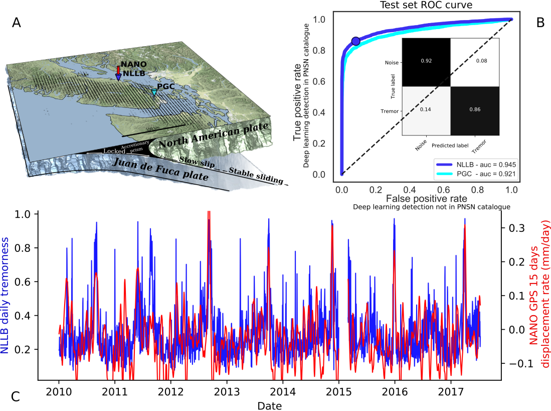
Figure 2: ‘Tremorness’ continuously tracks geodetic slow slip displacement rate, and generalizes to nearby stations. (A) Map of Vancouver Island. Slow slip and tremor originate from ductile portions of the interface, down dip from the locked zone where a megathrust earthquake is anticipated. Seismic stations NLLB and PGC as well as the GPS station NANO are noted by colored arrows. (B) The area under the receiving operating characteristic (ROC) curve and the confusion matrix. The ROC curve shows the true (deep learning detection of catalogued event) and false (deep learning detection of a possible but uncatalogued event) positive rates as the threshold of classification of the model is varied. A model that reproduces the catologue exactly would yield a point in the upper left corner or coordinate (0,1) of the ROC space. The inset shows the confusion matrix, indicating the fraction of classified noise and tremor by the deep learning model compared to the labels from the multi-station catalogue, for a model with a threshold of 0.5. Most tremor catalogued using multi-station cross-correlations are identified on a single station by the neural network. Other signals such as earthquakes, teleseisms, cultural noise and microseisms are easily distinguished from tremor by the model (see also Fig. S2). (C) Blue: daily average of the tremor content of the seismic data from the NLLB station, as determined by the deep learning model. Red: 15 days average of the co-located GPS displacement rate, from station NANO.

Given continuous seismic spectral data as input, the deep learning model outputs an empirical probability that the seismic data contains tectonic tremor. We term this empirical probability ‘tremorness’. We showed in previous work that the energy of continuously-recorded low-amplitude seismic waves track the smoothed GPS displacement rate well at long time scales (30+ days) and short time scales (one hour) [Rouet-Leduc . (2019)]. The energy-GPS correlation may suggest that tremor is emitted continuously or quasi-continuously at the plate interface from its slowly slipping portion (Fig. 2A). In contrast, catalogued tremor has been shown to be intermittent [Wech  Bartlow (2014)]. Using the deep CNN trained to recognize catalogued tremor, we find strong evidence that tremor is emitted at least quasi-continuously, and is a quantitative proxy for geodetic slow slip.

Figure 2C shows that the daily tremorness characteristic of the seismic data from the NLLB station tracks the co-located SW GPS displacement rate, even at small displacement rates and with modest GPS smoothing. In between the peaks of slow slip rate, the deep learning model finds that the seismic data on any given day contains 15 to 40% tremor (compared with 0.08% where no slow slip occurs, the actual false positive rate of our model, see Fig. S2). These weak tremors that go undetected in the multi-station method map to smaller peaks in the GPS displacement rate (see Fig. S4), demonstrating the possible existence of numerous slip events in between the known large slow slip events, as have been observed for instance in Mexico [Frank (2016)]. If we consider a detection threshold of tremor for a tremorness (CNN output) above 0.5 empirical probability, the default classifier built by the deep learning model, we detect more than 130,000 5-minute waveforms containing tremor events, close to three times the number contained in the catalog for the same time interval.

We note that our neural network has been trained to reproduce the catalogue as well as it could using a single seismic station. This corresponds to a threshold of 0.5 on the ROC curve on Fig. 2B. The deep learning model of tremor is therefore conservatively trained and the additional events it detects do not come from lowering the standards of detection compared to the multi-station method. This means that the model finds more events than those in the catalogue. This finding is not because these events correspond to a lower detection standard, but because according to the spectral features learned on a single station they are as likely to be tremor as the known catalogued events. These events are too weak in amplitude (see Fig. S3) to be detected on multiple stations, but based on the temporal evolution of their frequency content, the deep learning model cannot distinguish these newly detected tremor events from the known catalogued events. The correlation of tremorness and GPS displacement rate (Fig. 2C and S4) further demonstrates that these detections are not spurious. As a further test we applied the trained model to seismic data measured in a region known to be seismically inactive, in this case Michigan, USA (Fig., S2). Extremely little tremor is identified in Michigan by our model, supporting that the numerous newly detected tremor events in Cascadia are real. It also indicates that our model is not confused by cultural noise (e.g., train traffic, vehicular traffic, wind farms), meterological noise (wind, storms), or teleseisms.

Discussion

Deep learning model interpretation

Deep learning models are notoriously hard to interpret. However, recent efforts [Baehrens . (2010), Montavon . (2017)] have showed that perturbing the input of deep learning models enables their analysis, to some extent. In our case the network outputs the empirical probability that the input contains tremor, and a Taylor expansion of the model reveals the time-frequency components the network used to classify the signal as tremor. Fig.1D shows examples of such an analysis, applying a Taylor expansion of the neural network with respect to its input pixels [Montavon . (2017)] to construct a heatmap of time-frequency components identified used by the deep learning model to identify tremor. Fig.1E shows the inverse short-time Fourier transform of the time-frequency components identified as tremor by the Taylor analysis. Here, because the Taylor expansion identifies individual time-frequency components used to identify tremor, we can reconstruct a signal that represents the separation of the tremor signal from the background noise. We caution that this signal extraction method is only partial, as the Taylor expansion only reveals the time-frequency components that are characteristic of tremor, and not components that may be common between tremor and other signals.

The features learned by the convolutional neural network are patterns in the time-frequency domain, and we posit these features are directly related to the frictional properties of the slip on the interface that emit the signals. We presume that variations in pore pressure, chemistry, or thermal properties may modulate or influence the emitted signal, but the origin of the signal is due to emissions coming from asperities on the fault interface. In Fig. S5 we show evidence of the link between features learned by the CNN and inferred variations in frictional properties of the fault. The last feature map of the CNN, computed for classically catalogued and located tremor, exhibits a clustering in feature space that is reflected in its geographic location. This relation suggests that the tremor features learned by the CNN may be specific to the frictional properties of slip, as these features evolve systematically with the spatial origin of tremor. It is also possible the clustering results from distinct differences in path effects. This is a point we intend to explore further in future work, along with evolution of these features with time [Holtzman . (2018)].

Universality of tremor characteristics

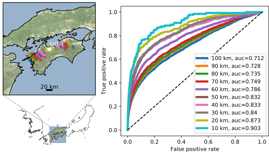
Figure 3: The deep neural network model of tremor trained in Cascadia recognizes known tremor in other regions. Left: Maps of catalogued tremor in Japan (A) and California (B). Right: ROC curves showing the accuracy of our model trained in Cascadia at recognizing tremor in Japan (A) and California (B), with colors matching. (A) ROC curves of the deep learning model of tremor exclusively trained in Cascadia, and applied to tremor catalogued in Shikoku, Japan [Ide (2012), Idehara . (2014)]. The performance decreases with distance (colors on maps and ROC curves matching). At short distances ($<$20 km) the model has the same performance on Japanese tremor as it does on Cascadia tremor. (B) ROC curves of the deep learning model applied to tremor catalogued on the San Andreas fault [Shelly (2017)]. The deep model trained on the Cascadia subduction zone only could not be used to build catalogues there on the San Andreas strike slip fault, but its ability to recognize catalogued tremor in most cases underscores the frictional similarity between strike slip tremor and subduction tremor.

Deep learning models have tremendous expression capabilities, which can lead to overfitting. In the previous section we demonstrated that our network generalizes to new seismic data from the station it was trained on, recorded later in time, suggesting that overfitting is not an issue. A powerful additional test is to see whether the network generalizes to seismic data from another station. Seismic recordings at a given station are a convolution of the source, propagation path and ‘site amplification’ effects, that may vary tremendously over short distances [Aki  Richards (2002)]. Generalization to another station would suggest that the network did not only learn the specifics of the seismic data it has been trained on. In Fig. 2B we show that our trained network is robust when applied to other seismic stations on Vancouver Island. The network trained on station NLLB from the end of 2009 to the end of 2015 can accurately recognize catalogued tremor on station PGC from 2016 to 2017, 80 km away. This test supports that the network did learn general time-frequency dynamics that are characteristic of tremor.

Furthermore, the model generalizes to other subduction zones and different tectonic environments (Fig. 3). Fig. 3A shows that catalogued tremor in Shikoku, southern Japan[Ide (2012), Idehara . (2014)] (also developed using multi-station envelope correlation) is accurately identified on a single station by our deep learning model of tremor trained in Cascadia, with no further training required. Fig. 3B shows that known tremor emitted by the San Andreas transform fault [Shelly (2017)] – a very different tectonic environment – is also identified by the same deep learning model trained in Cascadia. Tremor on the San Andreas fault has recently been shown to be due to slow slip on the deep portion of the fault [Rousset . (2019)], similar to slow slip in subduction zones. These results show that the time-frequency dynamics of tremor signals are largely dominated by the source characteristics, because our model is station and even region agnostic.

If tremor signals are dictated by source characteristics, then the time-frequency dynamics of these signals are indicative of an event rate and distribution that is characteristic of tremor: bursts of discrete events that are very similar in magnitude (very high b-values), with a very high event rate given by the time-frequency evolution of detected tremor. From this perspective, the time-frequency dynamics of tremor are a fingerprint of the frictional properties of the asperities that emit them. The ability of our model to recognize tremor in Japan and from the San Andreas fault suggests that the waveform characteristics of tremor are universal. This result is in line with laboratory analysis [Scuderi . (2016)] and models [Daub . (2011)] – tremor-inducing slow slip occurs within frictional conditions that are very similar for a wide variety of faults, and possibly all faults systems.

Conclusion

A deep learning model can be trained in Cascadia to accurately detect tectonic tremor on a single station. Trained on catalogued tremor events initially identified by multi-station methods, the deep learning model can be used to find many more events. The neural network gives a continuous measure of tremor content, that tracks geodetic displacement in Cascadia and provides clearer time bounds on slow slip events. Deep learning detection of tremor rises months before slow slip is detected geodetically. Trained only in Cascadia, the deep learning model recognizes known tremor from other subduction zones as well as from the deep portion of the San Andreas fault, arguing for the universality of the frictional properties governing slow earthquakes.

Data and code availability

The data used is publicly available and can be found online. The seismic data come from the Canadian National Seismograph Network [Canadian National Seismograph Network (1989)] (www.earthquakescanada. nrcan.gc.ca), and the GPS data come from the Western Canada Deformation Array (WCDA) operated by the Geological Survey of Canada (GSC), preprocessed by the USGS [Murray  Svarc (2017)]
(https://earthquake.usgs.gov/monitoring/gps/Pacific_Northwest, NA-fixed trended data). The known tremor catalog used is available from the Pacific Northwest Seismic Network (https://pnsn.org/tremor/tremor-map-legacy).

The work flow described in the Methods uses open source software: python and python packages including scikit-learn [Pedregosa . (2011)], tensorflow (https://www.tensorflow.org/), keras (https://keras.io/) and obspy [Beyreuther . (2010)].

References

- Aki \BBA Richards (\APACyear2002) \APACinsertmetastaraki2002quantitative{APACrefauthors}Aki, K.\BCBT \BBA Richards, P\BPBIG. \APACrefYearMonthDay2002. \BBOQ\APACrefatitleQuantitative seismology Quantitative seismology.\BBCQ \APACjournalVolNumPagesQuantitative Seismology, 2nd Ed., by Keiiti Aki and Paul G. Richards. Published by University Science Books, ISBN 0-935702-96-2, 704pp, 2002.. \PrintBackRefs\CurrentBib
- Baehrens \BOthers. (\APACyear2010) \APACinsertmetastarBaehrens2010{APACrefauthors}Baehrens, D., Schroeter, T., Harmeling, S., Kawanabe, M., Hansen, K.\BCBL \BBA Müller, K\BHBIR. \APACrefYearMonthDay2010. \BBOQ\APACrefatitleHow to Explain Individual Classification Decisions How to Explain Individual Classification Decisions.\BBCQ \APACjournalVolNumPagesJournal of Machine Learning Research11Jun1803–1831. \PrintBackRefs\CurrentBib
- Beyreuther \BOthers. (\APACyear2010) \APACinsertmetastarobspy{APACrefauthors}Beyreuther, M., Barsch, R., Krischer, L., Megies, T., Behr, Y.\BCBL \BBA Wassermann, J. \APACrefYearMonthDay2010. \BBOQ\APACrefatitleObsPy: A Python toolbox for seismology ObsPy: A Python toolbox for seismology.\BBCQ \APACjournalVolNumPagesSeismological Research Letters813530–533. \PrintBackRefs\CurrentBib
- \APACciteatitleCanadian National Seismograph Network (\APACyear1989) \APACinsertmetastarCNSN\BBOQ\APACrefatitleCanadian National Seismograph Network Canadian National Seismograph Network.\BBCQ \APACrefYearMonthDay1989. \APACjournalVolNumPagesGeological Survey of Canada. {APACrefDOI} 10.7914/SN/CN \PrintBackRefs\CurrentBib
- Daub \BOthers. (\APACyear2011) \APACinsertmetastarDaub2011{APACrefauthors}Daub, E\BPBIG., Shelly, D\BPBIR., Guyer, R\BPBIA.\BCBL \BBA Johnson, P\BPBIA. \APACrefYearMonthDay2011may. \BBOQ\APACrefatitleBrittle and ductile friction and the physics of tectonic tremor Brittle and ductile friction and the physics of tectonic tremor.\BBCQ \APACjournalVolNumPagesGeophysical Research Letters3810L10301. {APACrefDOI} 10.1029/2011GL046866 \PrintBackRefs\CurrentBib
- Frank (\APACyear2016) \APACinsertmetastarFrank2016{APACrefauthors}Frank, W\BPBIB. \APACrefYearMonthDay2016. \BBOQ\APACrefatitleSlow slip hidden in the noise: The intermittence of tectonic release Slow slip hidden in the noise: The intermittence of tectonic release.\BBCQ \APACjournalVolNumPagesGeophysical Research Letters431910,110–125,133. \PrintBackRefs\CurrentBib
- Frank \BBA Shapiro (\APACyear2014) \APACinsertmetastarFrank2014{APACrefauthors}Frank, W\BPBIB.\BCBT \BBA Shapiro, N\BPBIM. \APACrefYearMonthDay2014may. \BBOQ\APACrefatitleAutomatic detection of low-frequency earthquakes (LFEs) based on a beamformed network response Automatic detection of low-frequency earthquakes (LFEs) based on a beamformed network response.\BBCQ \APACjournalVolNumPagesGeophysical Journal International19721215–1223. {APACrefDOI} 10.1093/gji/ggu058 \PrintBackRefs\CurrentBib
- Gibbons \BBA Ringdal (\APACyear2006) \APACinsertmetastarGibbons2006{APACrefauthors}Gibbons, S\BPBIJ.\BCBT \BBA Ringdal, F. \APACrefYearMonthDay2006apr. \BBOQ\APACrefatitleThe detection of low magnitude seismic events using array-based waveform correlation The detection of low magnitude seismic events using array-based waveform correlation.\BBCQ \APACjournalVolNumPagesGeophysical Journal International1651149–166. {APACrefDOI} 10.1111/j.1365-246X.2006.02865.x \PrintBackRefs\CurrentBib
- Holtzman \BOthers. (\APACyear2018) \APACinsertmetastarHoltzman2018{APACrefauthors}Holtzman, B\BPBIK., Paté, A., Paisley, J., Waldhauser, F.\BCBL \BBA Repetto, D. \APACrefYearMonthDay2018may. \BBOQ\APACrefatitleMachine learning reveals cyclic changes in seismic source spectra in Geysers geothermal field Machine learning reveals cyclic changes in seismic source spectra in Geysers geothermal field.\BBCQ \APACjournalVolNumPagesScience Advances45eaao2929. {APACrefDOI} 10.1126/sciadv.aao2929 \PrintBackRefs\CurrentBib
- Ide (\APACyear2012) \APACinsertmetastarIde2012{APACrefauthors}Ide, S. \APACrefYearMonthDay2012mar. \BBOQ\APACrefatitleVariety and spatial heterogeneity of tectonic tremor worldwide Variety and spatial heterogeneity of tectonic tremor worldwide.\BBCQ \APACjournalVolNumPagesJournal of Geophysical Research: Solid Earth117B3. {APACrefDOI} 10.1029/2011JB008840 \PrintBackRefs\CurrentBib
- Idehara \BOthers. (\APACyear2014) \APACinsertmetastarIdehara2014{APACrefauthors}Idehara, K., Yabe, S.\BCBL \BBA Ide, S. \APACrefYearMonthDay2014dec. \BBOQ\APACrefatitleRegional and global variations in the temporal clustering of tectonic tremor activity New Perspective of Subduction Zone Earthquake Regional and global variations in the temporal clustering of tectonic tremor activity New Perspective of Subduction Zone Earthquake.\BBCQ \APACjournalVolNumPagesEarth, Planets and Space66166. {APACrefDOI} 10.1186/1880-5981-66-66 \PrintBackRefs\CurrentBib
- Ito \BOthers. (\APACyear2013) \APACinsertmetastarITO2013{APACrefauthors}Ito, Y., Hino, R., Kido, M., Fujimoto, H., Osada, Y., Inazu, D.\BDBLOthers \APACrefYearMonthDay2013. \BBOQ\APACrefatitleEpisodic slow slip events in the Japan subduction zone before the 2011 Tohoku-Oki earthquake Episodic slow slip events in the Japan subduction zone before the 2011 Tohoku-Oki earthquake.\BBCQ \APACjournalVolNumPagesTectonophysics60014–26. \PrintBackRefs\CurrentBib
- LeCun \BOthers. (\APACyear2015) \APACinsertmetastarLeCun2015{APACrefauthors}LeCun, Y., Bengio, Y.\BCBL \BBA Hinton, G. \APACrefYearMonthDay2015may. \BBOQ\APACrefatitleDeep learning Deep learning.\BBCQ \APACjournalVolNumPagesNature5217553436–444. {APACrefDOI} 10.1038/nature14539 \PrintBackRefs\CurrentBib
- Montavon \BOthers. (\APACyear2017) \APACinsertmetastarMontavon2017{APACrefauthors}Montavon, G., Lapuschkin, S., Binder, A., Samek, W.\BCBL \BBA Müller, K\BHBIR. \APACrefYearMonthDay2017may. \BBOQ\APACrefatitleExplaining nonlinear classification decisions with deep Taylor decomposition Explaining nonlinear classification decisions with deep Taylor decomposition.\BBCQ \APACjournalVolNumPagesPattern Recognition65211–222. {APACrefDOI} 10.1016/J.PATCOG.2016.11.008 \PrintBackRefs\CurrentBib
- Murray \BBA Svarc (\APACyear2017) \APACinsertmetastarUSGS{APACrefauthors}Murray, J\BPBIR.\BCBT \BBA Svarc, J. \APACrefYearMonthDay2017. \BBOQ\APACrefatitleGlobal Positioning System Data Collection, Processing, and Analysis Conducted by the U.S. Geological Survey Earthquake Hazards Program Global Positioning System Data Collection, Processing, and Analysis Conducted by the U.S. Geological Survey Earthquake Hazards Program.\BBCQ \APACjournalVolNumPagesSeismological Research Letters883916. \PrintBackRefs\CurrentBib
- Obara (\APACyear2002) \APACinsertmetastarObara2002{APACrefauthors}Obara, K. \APACrefYearMonthDay2002may. \BBOQ\APACrefatitleNonvolcanic deep tremor associated with subduction in southwest Japan Nonvolcanic deep tremor associated with subduction in southwest Japan.\BBCQ \APACjournalVolNumPagesScience29655731679–1681. {APACrefDOI} 10.1126/science.1070378 \PrintBackRefs\CurrentBib
- Obara \BBA Kato (\APACyear2016) \APACinsertmetastarObara2016{APACrefauthors}Obara, K.\BCBT \BBA Kato, A. \APACrefYearMonthDay2016jul. \BBOQ\APACrefatitleConnecting slow earthquakes to huge earthquakes Connecting slow earthquakes to huge earthquakes.\BBCQ \APACjournalVolNumPagesScience3536296253–257. {APACrefDOI} 10.1126/science.aaf1512 \PrintBackRefs\CurrentBib
- Pedregosa \BOthers. (\APACyear2011) \APACinsertmetastarPedregosa2011{APACrefauthors}Pedregosa, F., Varoquaux, G., Gramfort, A., Michel, V., Thirion, B., Grisel, O.\BDBLOthers \APACrefYearMonthDay2011. \BBOQ\APACrefatitleScikit-learn: Machine learning in Python Scikit-learn: Machine learning in Python.\BBCQ \APACjournalVolNumPagesJournal of Machine Learning Research12Oct2825–2830. \PrintBackRefs\CurrentBib
- Rogers \BBA Dragert (\APACyear2003) \APACinsertmetastarRogers2003{APACrefauthors}Rogers, G.\BCBT \BBA Dragert, H. \APACrefYearMonthDay2003. \BBOQ\APACrefatitleEpisodic tremor and slip on the Cascadia subduction zone: The chatter of silent slip Episodic tremor and slip on the Cascadia subduction zone: The chatter of silent slip.\BBCQ \APACjournalVolNumPagesScience30056271942–1943. \PrintBackRefs\CurrentBib
- Rouet-Leduc \BOthers. (\APACyear2019) \APACinsertmetastarRouet2019{APACrefauthors}Rouet-Leduc, B., Hulbert, C.\BCBL \BBA Johnson, P\BPBIA. \APACrefYearMonthDay2019jan. \BBOQ\APACrefatitle Continuous chatter of the Cascadia subduction zone revealed by machine learning Continuous chatter of the Cascadia subduction zone revealed by machine learning .\BBCQ \APACjournalVolNumPagesNature Geoscience121908–1752. {APACrefDOI} 10.1038/s41561-018-0274-6 \PrintBackRefs\CurrentBib
- Rousset \BOthers. (\APACyear2019) \APACinsertmetastarRousseteaav3274{APACrefauthors}Rousset, B., Bürgmann, R.\BCBL \BBA Campillo, M. \APACrefYearMonthDay2019feb. \BBOQ\APACrefatitleSlow slip events in the roots of the San Andreas fault Slow slip events in the roots of the San Andreas fault.\BBCQ \APACjournalVolNumPagesScience Advances52eaav3274. {APACrefDOI} 10.1126/sciadv.aav3274 \PrintBackRefs\CurrentBib
- Scuderi \BOthers. (\APACyear2016) \APACinsertmetastarScuderi2016{APACrefauthors}Scuderi, M\BPBIM., Marone, C., Tinti, E., Di Stefano, G.\BCBL \BBA Collettini, C. \APACrefYearMonthDay2016. \BBOQ\APACrefatitlePrecursory changes in seismic velocity for the spectrum of earthquake failure modes Precursory changes in seismic velocity for the spectrum of earthquake failure modes.\BBCQ \APACjournalVolNumPagesNature geoscience99695. \PrintBackRefs\CurrentBib
- Shelly (\APACyear2017) \APACinsertmetastarShelly2017{APACrefauthors}Shelly, D\BPBIR. \APACrefYearMonthDay2017may. \BBOQ\APACrefatitleA 15 year catalog of more than 1 million low-frequency earthquakes: Tracking tremor and slip along the deep San Andreas Fault A 15 year catalog of more than 1 million low-frequency earthquakes: Tracking tremor and slip along the deep San Andreas Fault.\BBCQ \APACjournalVolNumPagesJournal of Geophysical Research: Solid Earth12253739–3753. {APACrefDOI} 10.1002/2017JB014047 \PrintBackRefs\CurrentBib
- Vidale \BBA Houston (\APACyear2012) \APACinsertmetastarVidaleHouston{APACrefauthors}Vidale, J\BPBIE.\BCBT \BBA Houston, H. \APACrefYearMonthDay2012jan. \BBOQ\APACrefatitleSlow slip: A new kind of earthquake Slow slip: A new kind of earthquake.\BBCQ \APACjournalVolNumPagesPhysics Today65138–43. {APACrefDOI} 10.1063/PT.3.1399 \PrintBackRefs\CurrentBib
- Wech \BBA Bartlow (\APACyear2014) \APACinsertmetastarWechBartlow{APACrefauthors}Wech, A\BPBIG.\BCBT \BBA Bartlow, N\BPBIM. \APACrefYearMonthDay2014. \BBOQ\APACrefatitleSlip rate and tremor genesis in Cascadia Slip rate and tremor genesis in Cascadia.\BBCQ \APACjournalVolNumPagesGeophysical Research Letters412392–398. {APACrefDOI} 10.1002/2013GL058607 \PrintBackRefs\CurrentBib
- Wech \BBA Creager (\APACyear2008) \APACinsertmetastarwech2008{APACrefauthors}Wech, A\BPBIG.\BCBT \BBA Creager, K\BPBIC. \APACrefYearMonthDay2008. \BBOQ\APACrefatitleAutomated detection and location of Cascadia tremor Automated detection and location of Cascadia tremor.\BBCQ \APACjournalVolNumPagesGeophysical Research Letters3520. \PrintBackRefs\CurrentBib