New Physics in : Impact of Polarisation Observables and
Abstract
The experimental values of the lepton-flavour-universality tests and show a tension of about with their Standard Model prediction. Motivated by this tension, we perform a fit of the data. We consider one-particle scenarios imposing consecutive limits on , and analyse how these limits affect the fits. We include the polarisation observables available to date and predict those that are still to be measured, and conclude that they have a high model-resolving power. For each scenario we also predict , observing that an enhancement of implies an enhancement of in any scenario. We trace back this enhancement to a sum-rule valid irrespective of the scenario used to fit .
I Introduction
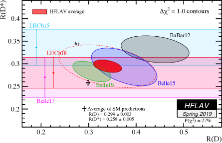
The lepton-flavour-universality tests , measured by the BaBar, Belle and LHCb collaborations Lees:2012xj ; Lees:2013uzd ; Huschle:2015rga ; Sato:2016svk ; Hirose:2016wfn ; Hirose:2017dxl ; Aaij:2015yra ; Aaij:2017uff ; Aaij:2017deq ; abd:2019dgh , are in tension with the Standard Model (SM) prediction with a combined difference of about . The average of the measurements can be found in Amhis:2016xyh , and Figure 1 displays a summary plot.
Data on the angular distribution of the final state particles in are also available from the Belle collaboration Hirose:2016wfn ; Hirose:2017dxl ; Adamczyk
In our analysis Blanke:2018yud ; Blanke:2019qrx we fitted these data to scenarios of new physics (NP) in which a single heavy mediator contributes to the transition , without contributing to the channels with a light lepton111For an analysis of NP effects in see Colangelo:2019axi ..
II New physics scenarios
The contributions of a NP mediator with mass above the meson mass to transitions, excluding the presence of light right-handed neutrinos, can be parametrised in terms of an effective field theory (EFT) as
| (1) |
with
| (2) |
The in the vectorial coupling represents the SM contribution, while all the remaining Wilson coefficients (WCs) encode only NP contributions.
The addition of a single NP particle to the SM can only give rise to a restricted subset of combinations of WCs. With the further assumption of real couplings, the parameters to fit are at most two. We can hence have the one-dimensional scenarios222For a discussion of the effects of a tensor coupling see Biancofiore:2013ki ; Colangelo:2016ymy ; Colangelo:2018cnj .:
-
•
: arising from the SU(2-singlet vector leptoquark (LQ) Alonso:2015sja ; Calibbi:2015kma ; Fajfer:2015ycq ; Barbieri:2015yvd ; Barbieri:2016las ; Hiller:2016kry ; Bhattacharya:2016mcc ; Buttazzo:2017ixm ; Kumar:2018kmr ; Assad:2017iib ; DiLuzio:2017vat ; Calibbi:2017qbu ; Bordone:2017bld ; Barbieri:2017tuq ; Blanke:2018sro ; Greljo:2018tuh ; Bordone:2018nbg ; Matsuzaki:2018jui ; Crivellin:2018yvo ; DiLuzio:2018zxy ; Biswas:2018snp , the scalar SU(2-triplet and/or scalar SU(2-singlet LQ Deshpande:2012rr ; Tanaka:2012nw ; Sakaki:2013bfa ; Freytsis:2015qca ; Bauer:2015knc ; Cai:2017wry ; Crivellin:2017zlb ; Altmannshofer:2017poe ; Marzocca:2018wcf with left-handed couplings only, or in models with left-handed bosons He:2012zp ; Greljo:2015mma ; Boucenna:2016wpr ; He:2017bft .
-
•
: arising from charged scalars or from the SU(2)L-doublet vector LQ Kosnik:2012dj ; Biswas:2018iak .
-
•
: arising from charged scalars in the hypothesis of a mechanism making the dominant operator Crivellin:2012ye ; Crivellin:2013wna ; Celis:2012dk ; Ko:2012sv ; Crivellin:2015hha ; Dhargyal:2016eri ; Chen:2017eby ; Iguro:2017ysu ; Martinez:2018ynq ; Biswas:2018jun .
-
•
: arising from the scalar SU(2-doublet (also called ) LQ Becirevic:2016yqi ; Becirevic:2018afm . Note that the relation holds at the NP scale, and gets modified by QCD and electroweak (EW) renormalization-group (RG) effects Alonso:2013hga ; Gonzalez-Alonso:2017iyc .
or the two-dimensional scenarios
-
•
: arising from the SU(2-singlet scalar LQ (). The relation holds again at the NP scale and must be evolved to the scale Gonzalez-Alonso:2017iyc .
-
•
: arising from charged scalars.
-
•
: arising from vector LQs like the SU(2-singlet LQ .
-
•
: as pointed out in Becirevic:2018afm , the scenario is able to reproduce the data only under the assumption of complex couplings. For this reason we also include it in the two-dimensional fits, fitting separately the real and the imaginary part.
III Constraints from
The vector () and pseudoscalar () couplings also mediate the decay Gonzalez-Alonso:2016etj ; Alonso:2016oyd . Although the branching ratio has not been measured yet, the comparison between the measured and SM-expected Gershtein:1994jw ; Bigi:1995fs ; Beneke:1996xe ; Chang:2000ac ; Kiselev:2000pp lifetime allows to set an upper limit on . This approach was used in Alonso:2016oyd to set an upper limit of . This limit can be relaxed if one takes into account the uncertainties in the theoretical calculation of the lifetime, originating from the large dependance on and from the calculation methods applied, namely heavy quark expansion and non-relativistic QCD (NRQCD).
Furthermore, the authors of Akeroyd:2017mhr set the upper limit using LEP data from an admixture of and and using the fragmentation functions ratio measured at hadron colliders, which have both different production mechanisms and different kinematics. Evaluating at the peak with by means of NRQCD mildens the constraint by a factor of . A more conservative estimate would further take the theoretical uncertainties into account.
In light of the above considerations, each NP scenario is analysed under three different assumptions: . These constraints are imposed as a hard cut on the region of parameter space allowed for the fit.
IV Fit results
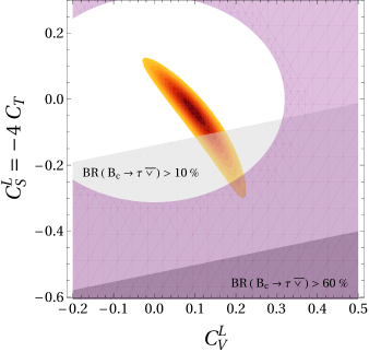
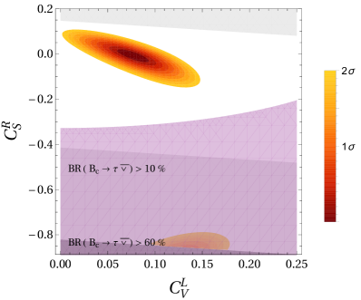
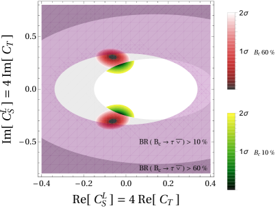
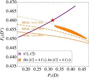
The results of the fits from Blanke:2019qrx are displayed in Tables 1, 2. The subscript, where present, refers to the limit on . Its absence indicates that the result does not change when changing the limit on . For each scenario we quote the goodness of fit in terms of -value and the pull of the best-fit point with the SM. The last six columns display the values of the observables at the best-fit point. For the measured ones () we also show the pull with respect to the experimental value. The one- and two- intervals for the 1D fits are displayed in Table 1, while the same regions for the 2D fits are plotted in Figure 2. The purple regions in scenarios are excluded at by collider bounds Greljo:2018tzh . These constraints are displayed as a dashed line for , since a collider study of this scenario requires a model-dependent analysis rather than an EFT one.
| 1D hyp. | best-fit | range | range | -value (%) | pullSM | ||||||
|---|---|---|---|---|---|---|---|---|---|---|---|
| 0.07 | [0.05, 0.09] | [0.04, 0.11] | 44 | 4.0 | 0.347 | 0.292 | 0.46 | 0.32 | 0.38 | ||
| 0.09 | [0.06, 0.11] | [0.03, 0.14] | 2.7 | 3.1 | 0.380 | 0.260 | 0.47 | 0.46 | 0.36 | ||
| 0.07 | [0.04, 0.10] | 0.26 | 2.1 | 0.364 | 0.250 | 0.45 | 0.44 | 0.35 | |||
|
|
[, ] | [, 0.04] | 0.04 | 0.7 | 0.278 | 0.263 | 0.46 | 0.27 | 0.33 |
| 2D hyp. | best-fit | -value (%) | pullSM | ||||||
|---|---|---|---|---|---|---|---|---|---|
| ( | 29.8 | 3.6 | 0.333 | 0.297 | 0.47 | 0.25 | 0.38 | ||
| ( | 75.7 | 3.9 | 0.338 | 0.297 | 0.54 | 0.39 | 0.38 | ||
| ( | 30.9 | 3.6 | 0.353 | 0.280 | 0.51 | 0.42 | 0.37 | ||
| ( | 2.6 | 2.9 | 0.366 | 0.263 | 0.48 | 0.44 | 0.36 | ||
| ( | 26.6 | 3.6 | 0.343 | 0.294 | 0.46 | 0.31 | 0.38 | ||
|
|
( | 25.0 | 3.6 | 0.339 | 0.295 0.0 | 0.45 | 0.41 | 0.38 | |
|
|
( | 5.9 | 3.2 | 0.330 | 0.275 | 0.46 | 0.38 | 0.36 |
Concerning , the most striking result from Table 2 is that with a limit, the scenario is the one preferred by the current experimental data. Its -value diminishes drastically as soon as we impose a more severe constraint. We conclude that a description of the anomaly in terms of charged Higgs predicts .
IV.1 Correlations between observables and sum rule
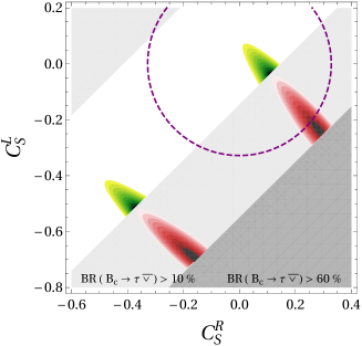
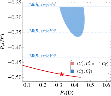
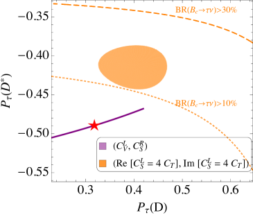
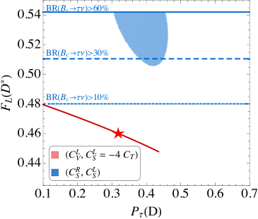
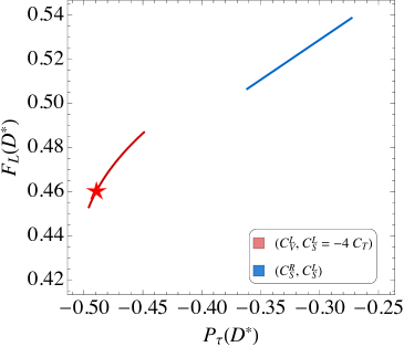
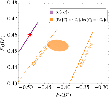
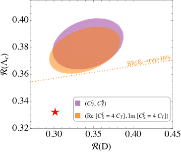
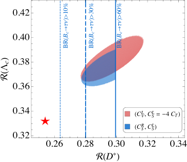
For the two dimensional scenario we also analysed the correlation between the observables in the last six columns of Table 2. In order to do so, we projected the two-sigma regions resulting from the fits with the limit into planes having as axes two out of the six observables. These plots are displayed in Figures 3 and 4 and allow us to draw two conclusions.
From Figure 3 we see that in planes in which one of the axes is a polarisation observable, the sigma regions of different scenarios separate clearly, hence indicating that these observables have a strong impact in distinguishing among models. In particular, a closer look at Table 2 reveals that the recent measurement of favours the scenario .
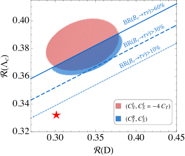
In Figure 4, instead, we see that the value of predicted in models fitting is always increased with respect to its SM prediction Detmold:2015aaa ; Bernlochner:2018bfn . This enhancement can be traced back to the sum rule
| (3) |
which holds irrespective of the NP model considered, and that can be understood in the heavy-quark limit. Substituting the current experimental averages of , we find
| (4) |
where the first error arises from the experimental uncertainty of , while the second comes from the form factors.

V Summary
Motivated by the anomaly, we updated the fit of data, including the recent experimental results from the Belle collaboration and restricting to scenarios with a single additional mediator. We revised the limit from and analysed its impact on each of the scenarios. The fit allowed us to appreciate the model-resolving power of polarisation observables, and to conclude that if the origin of the anomaly is new physics, we expect a value of higher than the one predicted by the Standard Model, irrespective of which additional particle mediates the decay.
Acknowledgements.
I am grateful to Monika Blanke, Andreas Crivellin, Stefan de Boer, Teppei Kitahara, Uli Nierste and Ivan Nišandžić for the fruitful collaboration that led to the results presented in this proceeding. I would also like to thank the organisers of the FPCP 2019 and to acknowledge the support of the DFG-funded Doctoral School KSETA and of the research training group GRK 1694.References
- (1) J. P. Lees et al. [BaBar Collaboration], Phys. Rev. Lett. 109 (2012) 101802 doi:10.1103/PhysRevLett.109.101802 [arXiv:1205.5442 [hep-ex]].
- (2) J. P. Lees et al. [BaBar Collaboration], Phys. Rev. D 88 (2013) no.7, 072012 doi:10.1103/PhysRevD.88.072012 [arXiv:1303.0571 [hep-ex]].
- (3) M. Huschle et al. [Belle Collaboration], Phys. Rev. D 92 (2015) no.7, 072014 doi:10.1103/PhysRevD.92.072014 [arXiv:1507.03233 [hep-ex]].
- (4) Y. Sato et al. [Belle Collaboration], Phys. Rev. D 94 (2016) no.7, 072007 doi:10.1103/PhysRevD.94.072007 [arXiv:1607.07923 [hep-ex]].
- (5) S. Hirose et al. [Belle Collaboration], Phys. Rev. Lett. 118 (2017) no.21, 211801 doi:10.1103/PhysRevLett.118.211801 [arXiv:1612.00529 [hep-ex]].
- (6) S. Hirose et al. [Belle Collaboration], Phys. Rev. D 97 (2018) no.1, 012004 doi:10.1103/PhysRevD.97.012004 [arXiv:1709.00129 [hep-ex]].
- (7) R. Aaij et al. [LHCb Collaboration], Phys. Rev. Lett. 115 (2015) no.11, 111803 Erratum: [Phys. Rev. Lett. 115 (2015) no.15, 159901] doi:10.1103/PhysRevLett.115.159901, 10.1103/PhysRevLett.115.111803 [arXiv:1506.08614 [hep-ex]].
- (8) R. Aaij et al. [LHCb Collaboration], Phys. Rev. Lett. 120 (2018) no.17, 171802 doi:10.1103/PhysRevLett.120.171802 [arXiv:1708.08856 [hep-ex]].
- (9) R. Aaij et al. [LHCb Collaboration], Phys. Rev. D 97 (2018) no.7, 072013 doi:10.1103/PhysRevD.97.072013 [arXiv:1711.02505 [hep-ex]].
- (10) A. Abdesselam et al. [Belle Collaboration], arXiv:1904.08794 [hep-ex].
-
(11)
Y. Amhis et al. [HFLAV Collaboration],
Eur. Phys. J. C 77 (2017) no.12, 895
doi:10.1140/epjc/s10052-017-5058-4
[arXiv:1612.07233 [hep-ex]].
Updated average of and for Spring 2019 at https://hflav-eos.web.cern.ch/hflav-eos/semi/spring19/html/RDsDsstar/RDRDs.html - (12) K. Adamczyk, ”B to semitauonic decays at Belle/Belle II”, Talk at 10th International Workshop on the CKM Unitarity Triangle, Heidelberg, 17-21 Sep 2018, https://indico.cern.ch/event/684284/timetable/#20180917.detailed.
- (13) M. Blanke, A. Crivellin, S. de Boer, T. Kitahara, M. Moscati, U. Nierste and I. Nišandžić, Phys. Rev. D 99 (2019) no.7, 075006 doi:10.1103/PhysRevD.99.075006 [arXiv:1811.09603 [hep-ph]].
- (14) M. Blanke, A. Crivellin, T. Kitahara, M. Moscati, U. Nierste and I. Nišandžić, arXiv:1905.08253 [hep-ph].
- (15) P. Colangelo, F. De Fazio and F. Loparco, arXiv:1906.07068 [hep-ph].
- (16) P. Biancofiore, P. Colangelo and F. De Fazio, Phys. Rev. D 87, no. 7, 074010 (2013) doi:10.1103/PhysRevD.87.074010 [arXiv:1302.1042 [hep-ph]].
- (17) P. Colangelo and F. De Fazio, Phys. Rev. D 95, no. 1, 011701 (2017) doi:10.1103/PhysRevD.95.011701 [arXiv:1611.07387 [hep-ph]].
- (18) P. Colangelo and F. De Fazio, JHEP 1806, 082 (2018) doi:10.1007/JHEP06(2018)082 [arXiv:1801.10468 [hep-ph]].
- (19) R. Alonso, B. Grinstein and J. Martin Camalich, JHEP 1510 (2015) 184 doi:10.1007/JHEP10(2015)184 [arXiv:1505.05164 [hep-ph]].
- (20) L. Calibbi, A. Crivellin and T. Ota, Phys. Rev. Lett. 115 (2015) 181801 doi:10.1103/PhysRevLett.115.181801 [arXiv:1506.02661 [hep-ph]].
- (21) S. Fajfer and N. Košnik, Phys. Lett. B 755 (2016) 270 doi:10.1016/j.physletb.2016.02.018 [arXiv:1511.06024 [hep-ph]].
- (22) R. Barbieri, G. Isidori, A. Pattori and F. Senia, Eur. Phys. J. C 76 (2016) no.2, 67 doi:10.1140/epjc/s10052-016-3905-3 [arXiv:1512.01560 [hep-ph]].
- (23) R. Barbieri, C. W. Murphy and F. Senia, Eur. Phys. J. C 77 (2017) no.1, 8 doi:10.1140/epjc/s10052-016-4578-7 [arXiv:1611.04930 [hep-ph]].
- (24) G. Hiller, D. Loose and K. Schönwald, JHEP 1612 (2016) 027 doi:10.1007/JHEP12(2016)027 [arXiv:1609.08895 [hep-ph]].
- (25) B. Bhattacharya, A. Datta, J. P. Guévin, D. London and R. Watanabe, JHEP 1701 (2017) 015 doi:10.1007/JHEP01(2017)015 [arXiv:1609.09078 [hep-ph]].
- (26) D. Buttazzo, A. Greljo, G. Isidori and D. Marzocca, JHEP 1711 (2017) 044 doi:10.1007/JHEP11(2017)044 [arXiv:1706.07808 [hep-ph]].
- (27) J. Kumar, D. London and R. Watanabe, Phys. Rev. D 99 (2019) no.1, 015007 doi:10.1103/PhysRevD.99.015007 [arXiv:1806.07403 [hep-ph]].
- (28) N. Assad, B. Fornal and B. Grinstein, Phys. Lett. B 777 (2018) 324 doi:10.1016/j.physletb.2017.12.042 [arXiv:1708.06350 [hep-ph]].
- (29) L. Di Luzio, A. Greljo and M. Nardecchia, Phys. Rev. D 96 (2017) no.11, 115011 doi:10.1103/PhysRevD.96.115011 [arXiv:1708.08450 [hep-ph]].
- (30) L. Calibbi, A. Crivellin and T. Li, Phys. Rev. D 98 (2018) no.11, 115002 doi:10.1103/PhysRevD.98.115002 [arXiv:1709.00692 [hep-ph]].
- (31) M. Bordone, C. Cornella, J. Fuentes-Martin and G. Isidori, Phys. Lett. B 779 (2018) 317 doi:10.1016/j.physletb.2018.02.011 [arXiv:1712.01368 [hep-ph]].
- (32) R. Barbieri and A. Tesi, Eur. Phys. J. C 78 (2018) no.3, 193 doi:10.1140/epjc/s10052-018-5680-9 [arXiv:1712.06844 [hep-ph]].
- (33) M. Blanke and A. Crivellin, Phys. Rev. Lett. 121 (2018) no.1, 011801 doi:10.1103/PhysRevLett.121.011801 [arXiv:1801.07256 [hep-ph]].
- (34) A. Greljo and B. A. Stefanek, Phys. Lett. B 782 (2018) 131 doi:10.1016/j.physletb.2018.05.033 [arXiv:1802.04274 [hep-ph]].
- (35) M. Bordone, C. Cornella, J. Fuentes-Martín and G. Isidori, JHEP 1810 (2018) 148 doi:10.1007/JHEP10(2018)148 [arXiv:1805.09328 [hep-ph]].
- (36) S. Matsuzaki, K. Nishiwaki and K. Yamamoto, JHEP 1811 (2018) 164 doi:10.1007/JHEP11(2018)164 [arXiv:1806.02312 [hep-ph]].
- (37) A. Crivellin, C. Greub, D. Müller and F. Saturnino, Phys. Rev. Lett. 122 (2019) no.1, 011805 doi:10.1103/PhysRevLett.122.011805 [arXiv:1807.02068 [hep-ph]].
- (38) L. Di Luzio, J. Fuentes-Martin, A. Greljo, M. Nardecchia and S. Renner, JHEP 1811 (2018) 081 doi:10.1007/JHEP11(2018)081 [arXiv:1808.00942 [hep-ph]].
- (39) A. Biswas, D. Kumar Ghosh, N. Ghosh, A. Shaw and A. K. Swain, arXiv:1808.04169 [hep-ph].
- (40) N. G. Deshpande and A. Menon, JHEP 1301 (2013) 025 doi:10.1007/JHEP01(2013)025 [arXiv:1208.4134 [hep-ph]].
- (41) M. Tanaka and R. Watanabe, Phys. Rev. D 87 (2013) no.3, 034028 doi:10.1103/PhysRevD.87.034028 [arXiv:1212.1878 [hep-ph]].
- (42) Y. Sakaki, M. Tanaka, A. Tayduganov and R. Watanabe, Phys. Rev. D 88 (2013) no.9, 094012 doi:10.1103/PhysRevD.88.094012 [arXiv:1309.0301 [hep-ph]].
- (43) M. Freytsis, Z. Ligeti and J. T. Ruderman, Phys. Rev. D 92 (2015) no.5, 054018 doi:10.1103/PhysRevD.92.054018 [arXiv:1506.08896 [hep-ph]].
- (44) M. Bauer and M. Neubert, Phys. Rev. Lett. 116 (2016) no.14, 141802 doi:10.1103/PhysRevLett.116.141802 [arXiv:1511.01900 [hep-ph]].
- (45) Y. Cai, J. Gargalionis, M. A. Schmidt and R. R. Volkas, JHEP 1710 (2017) 047 doi:10.1007/JHEP10(2017)047 [arXiv:1704.05849 [hep-ph]].
- (46) A. Crivellin, D. Müller and T. Ota, JHEP 1709 (2017) 040 doi:10.1007/JHEP09(2017)040 [arXiv:1703.09226 [hep-ph]].
- (47) W. Altmannshofer, P. S. Bhupal Dev and A. Soni, Phys. Rev. D 96 (2017) no.9, 095010 doi:10.1103/PhysRevD.96.095010 [arXiv:1704.06659 [hep-ph]].
- (48) D. Marzocca, JHEP 1807 (2018) 121 doi:10.1007/JHEP07(2018)121 [arXiv:1803.10972 [hep-ph]].
- (49) X. G. He and G. Valencia, Phys. Rev. D 87 (2013) no.1, 014014 doi:10.1103/PhysRevD.87.014014 [arXiv:1211.0348 [hep-ph]].
- (50) A. Greljo, G. Isidori and D. Marzocca, JHEP 1507 (2015) 142 doi:10.1007/JHEP07(2015)142 [arXiv:1506.01705 [hep-ph]].
- (51) S. M. Boucenna, A. Celis, J. Fuentes-Martin, A. Vicente and J. Virto, Phys. Lett. B 760 (2016) 214 doi:10.1016/j.physletb.2016.06.067 [arXiv:1604.03088 [hep-ph]].
- (52) X. G. He and G. Valencia, Phys. Lett. B 779 (2018) 52 doi:10.1016/j.physletb.2018.01.073 [arXiv:1711.09525 [hep-ph]].
- (53) N. Kosnik, Phys. Rev. D 86 (2012) 055004 doi:10.1103/PhysRevD.86.055004 [arXiv:1206.2970 [hep-ph]].
- (54) A. Biswas, A. Shaw and A. K. Swain, arXiv:1811.08887 [hep-ph].
- (55) A. Crivellin, C. Greub and A. Kokulu, Phys. Rev. D 86 (2012) 054014 doi:10.1103/PhysRevD.86.054014 [arXiv:1206.2634 [hep-ph]].
- (56) A. Crivellin, A. Kokulu and C. Greub, Phys. Rev. D 87 (2013) no.9, 094031 doi:10.1103/PhysRevD.87.094031 [arXiv:1303.5877 [hep-ph]].
- (57) A. Celis, M. Jung, X. Q. Li and A. Pich, JHEP 1301 (2013) 054 doi:10.1007/JHEP01(2013)054 [arXiv:1210.8443 [hep-ph]].
- (58) P. Ko, Y. Omura and C. Yu, JHEP 1303 (2013) 151 doi:10.1007/JHEP03(2013)151 [arXiv:1212.4607 [hep-ph]].
- (59) A. Crivellin, J. Heeck and P. Stoffer, Phys. Rev. Lett. 116 (2016) no.8, 081801 doi:10.1103/PhysRevLett.116.081801 [arXiv:1507.07567 [hep-ph]].
- (60) L. Dhargyal, Phys. Rev. D 93 (2016) no.11, 115009 doi:10.1103/PhysRevD.93.115009 [arXiv:1605.02794 [hep-ph]].
- (61) C. H. Chen and T. Nomura, Eur. Phys. J. C 77 (2017) no.9, 631 doi:10.1140/epjc/s10052-017-5198-6 [arXiv:1703.03646 [hep-ph]].
- (62) S. Iguro and K. Tobe, Nucl. Phys. B 925 (2017) 560 doi:10.1016/j.nuclphysb.2017.10.014 [arXiv:1708.06176 [hep-ph]].
- (63) R. Martinez, C. F. Sierra and G. Valencia, Phys. Rev. D 98 (2018) no.11, 115012 doi:10.1103/PhysRevD.98.115012 [arXiv:1805.04098 [hep-ph]].
- (64) A. Biswas, D. K. Ghosh, S. K. Patra and A. Shaw, arXiv:1801.03375 [hep-ph].
- (65) D. Bečirević, S. Fajfer, N. Košnik and O. Sumensari, Phys. Rev. D 94 (2016) no.11, 115021 doi:10.1103/PhysRevD.94.115021 [arXiv:1608.08501 [hep-ph]].
- (66) D. Bečirević, I. Doršner, S. Fajfer, N. Košnik, D. A. Faroughy and O. Sumensari, Phys. Rev. D 98 (2018) no.5, 055003 doi:10.1103/PhysRevD.98.055003 [arXiv:1806.05689 [hep-ph]].
- (67) R. Alonso, E. E. Jenkins, A. V. Manohar and M. Trott, JHEP 1404 (2014) 159 doi:10.1007/JHEP04(2014)159 [arXiv:1312.2014 [hep-ph]].
- (68) M. González-Alonso, J. Martin Camalich and K. Mimouni, Phys. Lett. B 772 (2017) 777 doi:10.1016/j.physletb.2017.07.003 [arXiv:1706.00410 [hep-ph]].
- (69) M. González-Alonso and J. Martin Camalich, JHEP 1612 (2016) 052 doi:10.1007/JHEP12(2016)052 [arXiv:1605.07114 [hep-ph]].
- (70) R. Alonso, B. Grinstein and J. Martin Camalich, Phys. Rev. Lett. 118 (2017) no.8, 081802 doi:10.1103/PhysRevLett.118.081802 [arXiv:1611.06676 [hep-ph]].
- (71) S. S. Gershtein, V. V. Kiselev, A. K. Likhoded and A. V. Tkabladze, Phys. Usp. 38 (1995) 1 [Usp. Fiz. Nauk 165 (1995) 3] doi:10.1070/PU1995v038n01ABEH000063 [hep-ph/9504319].
- (72) I. I. Y. Bigi, Phys. Lett. B 371, 105 (1996) doi:10.1016/0370-2693(95)01574-4 [hep-ph/9510325].
- (73) M. Beneke and G. Buchalla, Phys. Rev. D 53 (1996) 4991 doi:10.1103/PhysRevD.53.4991 [hep-ph/9601249].
- (74) C. H. Chang, S. L. Chen, T. F. Feng and X. Q. Li, Phys. Rev. D 64 (2001) 014003 doi:10.1103/PhysRevD.64.014003 [hep-ph/0007162].
- (75) V. V. Kiselev, A. E. Kovalsky and A. K. Likhoded, Nucl. Phys. B 585 (2000) 353 doi:10.1016/S0550-3213(00)00386-2 [hep-ph/0002127].
- (76) A. G. Akeroyd and C. H. Chen, Phys. Rev. D 96 (2017) no.7, 075011 doi:10.1103/PhysRevD.96.075011 [arXiv:1708.04072 [hep-ph]].
- (77) A. Greljo, J. Martin Camalich and J. D. Ruiz-Álvarez, Phys. Rev. Lett. 122 (2019) no.13, 131803 doi:10.1103/PhysRevLett.122.131803 [arXiv:1811.07920 [hep-ph]].
- (78) W. Detmold, C. Lehner and S. Meinel, Phys. Rev. D 92 (2015) no.3, 034503 doi:10.1103/PhysRevD.92.034503 [arXiv:1503.01421 [hep-lat]].
- (79) F. U. Bernlochner, Z. Ligeti, D. J. Robinson and W. L. Sutcliffe, Phys. Rev. D 99 (2019) no.5, 055008 doi:10.1103/PhysRevD.99.055008 [arXiv:1812.07593 [hep-ph]].