Controllability of periodic bilinear quantum systems on infinite graphs

Abstract.

In this work, we study the controllability of the bilinear Schrödinger equation on infinite graphs for periodic quantum states. We consider the bilinear Schrödinger equation (BSE) $i\partial_{t}\psi=-\Delta\psi+u(t)B\psi$ in the Hilbert space $L^{2}_{p}$ composed by functions defined on an infinite graph $\mathscr{G}$ verifying periodic boundary conditions on the infinite edges. The Laplacian $-\Delta$ is equipped with specific boundary conditions, $B$ is a bounded symmetric operator and $u\in L^{2}((0,T),\mathbb{R})$ with $T>0$. We present the well-posedness of the (BSE) in suitable subspaces of $D(|\Delta|^{3/2})$ . In such spaces, we study the global exact controllability and we provide examples involving tadpole graphs and star graphs with infinite spokes.

1. Introduction

Graph type structures (Figure 1) have been widely studied for the modeling of phenomena arising in science, social sciences and engineering. Among the many applications to quantum mechanics, they were used to study the dynamics of free electrons in organic molecules starting from the seminal work [37], the superconductivity in granular and artificial materials [1], acoustic and electromagnetic wave-guides networks in [25, 32], etc.

Figure 1. An infinite graph is an one-dimensional domain composed by vertices (points) connected by edges (segments and half-lines).

We consider a particle trapped on a network of wave-guides or wires where some branches are way longer than the others. We model the long branches with half-lines and the remaining ones with segments in order to represent the network by an infinite graph. The nodes of the network are ideal so that the crossing particle is subjected to zero resistance during the motion and we assume that the system is subjected to an external field which plays the role of control.

A natural choice for such setting is to represent the network by an infinite graph $\mathscr{G}$ and the state of the particle by a function $\psi$ with domain $\mathscr{G}$. The state $\psi$ belongs to a suitable Hilbert space $\mathscr{H}$ and the dynamics of the particle is modeled by the bilinear Schrödinger equation in $\mathscr{H}$

$$i\partial_{t}\psi(t,x)=A\psi(t,x)+u(t)B\psi(t,x),\ \ \ \ \ \ t\in[0,T],\ x\in\mathscr{G},$$ (1)

where $A$ is a positive self-adjoint operator. The term $u(t)B$ represents the time dependent external field acting on the system which action is given by the bounded symmetric operator $B$ and its intensity by the control function $u\in L^{2}((0,T),\mathbb{R})$.

In this work, we consider $\mathscr{H}$ as the Hilbert space composed by $L^{2}_{loc}$ functions over the graph satisfying periodic boundary conditions on the infinite edges and $A$ is a Laplacian equipped with suitable boundary conditions. We study the controllability of the bilinear Schrödinger equation (1) according to the choice of the graph. Our purpose is to analyze when it is possible to control exactly the motion by time-varying the intensity of the external field.

Some bibliography

The mathematical analysis of operators defined on networks was preliminarily addressed in [39] by Ruedenber and Scherr. In this work, they studied the dynamics of particular electrons in the conjugated double-bounds organic molecules. These particles move as if they were trapped on a network of wave-guides and the graphs are obtained as the idealization of such structures in the limit where the diameter of the section is much smaller than the length. A similar approach was developed by Saito in [40, 41] where the graphs are obtained as “shrinking” domains. For analogous ideas, we refer to the papers [36, 38].

The controllability of finite-dimensional quantum systems modeled by equations as (1), when $A$ and $B$ are $N\times N$ Hermitian matrices, is well-known for being linked to the rank of the Lie algebra spanned by $A$ and $B$ (see [4, 19]). Nevertheless, the Lie algebra rank condition can not be used for infinite-dimensional quantum systems (see [19]).

The global approximate controllability of the bilinear Schrödinger equations (1) was proved with different techniques in literature. We refer to [31, 35] for Lyapunov techniques, to [15, 16] for adiabatic arguments and to [14, 17] for Lie-Galerking methods.

The exact controllability of infinite-dimensional quantum systems is in general more delicate. For instance, the controllability and observability of the linear Schrödinger equation are reciprocally dual. Various results were developed by addressing directly or by duality the control problem with multiplier methods [28, 29], microlocal analysis [9, 18, 27] and Carleman estimates [10, 26, 30]. However, a complete theory on networks is far from being formulated. Indeed, the interaction between the different components of the structure may generate unexpected phenomena. For further details on the subject, we refer to [20].

An important property of the bilinear Schrödinger equation is that its controllability can not be approached with the techniques valid for the linear Schrödinger equation. Indeed, the dynamics of (1) is well-known for not being exactly controllable in the Hilbert space $\mathscr{H}$ where it is defined when $B$ is a bounded operator and $u\in L^{2}((0,T),\mathbb{R})$ with $T>0$ (even though it is well-posed in such space). This result was proved by Turinici in [42] by exploiting the theory developed by Ball, Mardsen and Slemrod in [6] (see [7, 8] for other results on bilinear systems). As a consequence, the classical techniques can not be exploited for the exact controllability of bilinear quantum systems.

The turning point for this kind of studies has been the idea of controlling the equation in specific subspaces of $D(A)$. Preliminarily introduced by Beauchard in [11], this approach was mostly popularized by the work [13] of Beauchard and Laurent. There, they considered the bilinear Schrödinger equation $\eqref{eq1}$ on the interval $\mathscr{G}=(0,1)$ when $\mathscr{H}=L^{2}((0,1),\mathbb{C})$, $B$ is a suitable multiplication operator and $A=-\Delta_{D}$ is the Dirichlet Laplacian

$$D(-\Delta_{D})=H^{2}((0,1),\mathbb{C})\cap H^{1}_{0}((0,1),\mathbb{C})),\ \ \ \ \ -\Delta_{D}\psi:=-\Delta\psi,\ \ \ \ \forall\psi\in D(-\Delta_{D}).$$

They proved the well-posedness and the local exact controllability of the equation in the space $D(|\Delta_{D}|^{3/2})$. Afterwards, different works on the subject were developed. We refer to [12, 22] for global exact controllability results and [22, 33, 34] for simultaneous exact controllability results.

The controllability of bilinear quantum systems on graphs was preliminarily addressed by the second author in [21, 23]. There, the bilinear Schrödinger equation (1) is considered in the Hilbert space $L^{2}(\mathscr{G},\mathbb{C})$ with $\mathscr{G}$ a compact graph and $A$ a suitable self-adjoint Laplacian. One of the main difficulties of this framework is due to the nature of the spectrum of $A$. In particular, when we consider its ordered sequence of eigenvalues $(\lambda_{k})_{k\in\mathbb{N}^{*}}$, it is possible to show that there exists $\mathcal{M}\in\mathbb{N}^{*}$ such that

$$\begin{split}\inf_{{k\in\mathbb{N}^{*}}}|\lambda_{k+\mathcal{M}}-\lambda_{k}|>0\\ \end{split}$$ (2)

(as ensured in [21, Lemma 2.4]). Nevertheless, the uniform spectral gap $\inf_{{k\in\mathbb{N}^{*}}}|\lambda_{k+1}-\lambda_{k}|>0$ is only valid when $\mathscr{G}=(0,1)$. This hypothesis was crucial for the techniques adopted in the previous works on bounded intervals, which could not be applied in this framework. To this purpose, new spectral techniques were developed in the works [21, 23] in order to ensure the global exact controllability of the bilinear Schrödinger equation (1) on compact graphs.

When we consider the bilinear Schrödinger equation (1) on infinite graphs instead, a natural obstacle to the controllability is the loss of localization of the wave packets during the evolution: the dispersion. This effect can be measured by $L^{\infty}$-time decay, which implies a spreading out of the solutions, due to the time invariance of the $L^{2}$-norm. Dispersive estimations on infinite graphs can be found in [2, 3]. The other side of the same coin is that a self-adjoint Laplacian $A$ on $L^{2}(\mathscr{G},\mathbb{C})$ where $\mathscr{G}$ is an infinite graph, does not admit compact resolvent and then, the spectral techniques from [21, 23] can not be directly applied to this framework.

Despite the dispersive behavior of the bilinear Schrödinger equation (1) on infinite graphs, the authors addressed the problem in [5] by exploiting a simple but still effective idea. When $\mathscr{G}$ contains suitable substructures, the Laplacian $A$ admits discrete spectrum corresponding to some specific eigenmodes. Such states are preserved by the dynamics of (1) for suitable choices of $B$ and they are not affected by the dispersive behavior of the equation. By working on the space spanned by such eigenmodes, global exact controllability results for the equation (1) can be ensured in suitable subspaces of $L^{2}(\mathscr{G},\mathbb{C})$ with $\mathscr{G}$ an infinite graph, as presented in [5]. We underline that the considered eigenmodes are supported in compact sub-graphs of $\mathscr{G}$ and then, the result is only valid for suitable states vanishing on the infinite edges of the graph.

From this perspective, our purpose is natural. We aim to carry on the existing theory by proving the controllability of (1) for quantum states that do not vanish on the infinite edges of the graph. In this regard, we consider the bilinear Schrödinger equation (1) for periodic functions. This choice allows us to have non-compactly supported eigenmodes and then, to ensure the exact controllability for states also defined on the infinite edges of the graph.

Scheme of the work

The paper is organized as follows. In Section 2, we introduce the main notations of the work. In Sections 3 and Section 4, we respectively prove the global exact controllability when $\mathscr{G}$ is an infinite tadpole graph and an infinite star graph. In the last section, we generalize the previous results to some general infinite graphs.

2. Preliminaries

Let $\mathscr{G}$ be a general graph composed by $N$ finite edges $\{e_{j}\}_{1\leq j\leq N}$ of lengths $\{L_{j}\}_{1\leq j\leq N}$ and $\widetilde{N}$ half-lines $\{e_{j}\}_{N+1\leq j\leq N+\widetilde{N}}$. Each edge $e_{j}$ with $j\leq N$ is associated to a coordinate starting from $0$ and going to $L_{j}$, while $e_{j}$ with $N+1\leq j\leq N+\widetilde{N}$ is parametrized with a coordinate starting from $0$ and going to $+\infty$. We consider $\mathscr{G}$ as domain of functions

$$f:=(f^{1},...,f^{N+\widetilde{N}}):\mathscr{G}\rightarrow\mathbb{C},\ \ \ \ \ \ \ \ \ f^{j}:e_{j}\rightarrow\mathbb{C},\ \ \ \ \ 1\leq j\leq N+\widetilde{N}.$$

Let $\{L_{j}\}_{N+1\leq j\leq N+\widetilde{N}}\subset\mathbb{R}^{+}$. We consider the Hilbert space

$$L^{2}_{p}:=L^{2}_{p}(\mathscr{G},\mathbb{C})=\Big{(}\prod_{j=1}^{N}L^{2}(e_{j},\mathbb{C})\Big{)}\times\Big{(}\prod_{j=N+1}^{N+\widetilde{N}}L^{2}_{p}(e_{j},\mathbb{C})\Big{)},\ \ \ \ \ \text{with}$$ (3)

$$L^{2}_{p}(e_{j},\mathbb{C})=\Big{\{}f\in L^{2}_{loc}(e_{j},\mathbb{C})\ :\ f(\cdot)=f\big{(}\ \cdot\ +2\pi kL_{j}\big{)},\ \ \ \ \forall k\in\mathbb{N}^{*}\Big{\}},\ \ \ N+1\leq j\leq N+\widetilde{N}.$$

The Hilbert spaces $L^{2}_{p}$ is equipped with the norm $\|\cdot\|_{L^{2}_{p}}$ induced by the scalar product

$$\langle\psi,\varphi\rangle_{L^{2}_{p}}=\sum_{j=1}^{N+\widetilde{N}}\int_{0}^{L_{j}}\overline{\psi^{j}}(x)\varphi^{j}(x)dx,\ \ \ \ \ \ \forall\psi,\varphi\in L^{2}_{p}.$$

We introduce the spaces

$$H^{s}_{p}:=L^{2}_{p}\cap\Bigg{(}\Big{(}\prod_{j=1}^{N}H^{s}(e_{j},\mathbb{C})\Big{)}\times\Big{(}\prod_{j=N+1}^{N+\widetilde{N}}H^{s}_{loc}(e_{j},\mathbb{C})\Big{)}\Bigg{)}$$

with $s>0$. For $T>0$, we consider the bilinear Schrödinger equation in $L^{2}_{p}$

$$\begin{split}\begin{cases}i\partial_{t}\psi(t)=-A\psi(t)+u(t)B\psi(t),\ \ \ \ \ \ \ \ &t\in(0,T),\\ \psi(0)=\psi_{0}.\\ \end{cases}\end{split}$$ (BSE)

The operator $A$ is a Laplacian equipped with suitable boundary conditions such that $D(A)\subseteq H^{2}_{p}$. The operator $B$ is a bounded symmetric operator in $L^{2}_{p}$ and $u\in L^{2}((0,T),\mathbb{R})$ with $T>0$. We respectively denote

$$\upvarphi:=\{\varphi_{k}\}_{k\in\mathbb{N}^{*}},\ \ \ \ \ \ \ \ \ \ \ \ \upmu:=\{\mu_{k}\}_{k\in\mathbb{N}^{*}}$$

an orthonormal system of $L^{2}_{p}$ made by some eigenfunctions of $A$ and the corresponding eigenvalues. For $s>0$, we define the spaces

$$\mathscr{H}(\upvarphi):=\overline{span\{\varphi_{k}\ |\ k\in\mathbb{N}^{*}\}}^{\ L^{2}_{p}},$$

$$\begin{split}&H^{s}_{\mathscr{G}}(\upvarphi):=\{\psi\in\mathscr{H}(\upvarphi)\ |\ \sum_{k\in\mathbb{N}^{*}}|k^{s}\langle\varphi_{k},\psi\rangle_{L^{2}_{p}}|^{2}<\infty\},\\ &h^{s}:=\Big{\{}\{a_{k}\}_{k\in\mathbb{N}^{*}}\in\ell^{2}(\mathbb{C})\ \big{|}\ \sum_{k\in\mathbb{N}^{*}}|k^{s}a_{k}|^{2}<\infty\Big{\}}.\\ \end{split}$$ (4)

We respectively equip $H^{s}_{\mathscr{G}}(\upvarphi)$ and $h^{s}$ with the norms $\|\cdot\|_{(s)}=\big{(}{\sum_{k\in\mathbb{N}^{*}}}|k^{s}\langle\varphi_{k},\cdot\rangle_{L^{2}_{p}}|^{2}\big{)}^{\frac{1}{2}}$ and

$$\|{\bf x}\|_{(s)}=\big{(}\sum_{k\in\mathbb{N}^{*}}|k^{s}x_{k}|^{2}\big{)}^{\frac{1}{2}},\ \ \ \ \ \ \ \ \ \forall{\bf x}:=(x_{k})_{k\in\mathbb{N}^{*}}\in h^{s}.$$

Remark.

The space $\mathscr{H}(\upvarphi)$ is usually strictly smaller than $L^{2}_{p}$. If for instance we consider $\mathscr{G}$ as a ring parametrized from $0$ to $1$ and $\upvarphi=\big{\{}\sqrt{2}\sin(2k\pi x)\big{\}}_{k\in\mathbb{N}^{*}}$, then $\mathscr{H}(\upvarphi)$ is composed by those $L^{2}_{p}$ states which are odd with respect to the point $x=1/2$ and clearly $\mathscr{H}(\upvarphi)\subset L_{p}^{2}.$

Remark.

Let $\mu_{k}\sim k^{2}$ and $c\in\mathbb{R}^{+}$ be such that $0\not\in\sigma(A+c,\mathscr{H}(\upvarphi))$ (the spectrum of $A+c$ in the Hilbert space $\mathscr{H}(\upvarphi)$). For every $s>0,$ there exist $C_{1},C_{2}>0$ such that

$$C_{1}\|\psi\|_{(s)}\leq\||A+c|^{s/2}\psi\|_{L^{2}_{p}}\leq C_{2}\|\psi\|_{(s)},\ \ \ \ \ \ \ \ \forall\psi\in H^{s}_{\mathscr{G}}(\upvarphi).$$

Let $\Gamma_{T}^{u}$ be the unitary propagator (when it is defined) corresponding to the dynamics of (BSE) in the time interval $[0,T]$.

Definition 2.1.

Let $\upvarphi$ be an orthonormal system of $L^{2}_{p}$ made by some eigenfunctions of $A$ and $s>0$. The bilinear Schrödinger equation (BSE) is said to be globally exactly controllable in $H^{s}_{\mathscr{G}}(\upvarphi)$ when, for every $\psi_{1},\psi_{2}\in H^{s}_{\mathscr{G}}(\upvarphi)$ such that $\|\psi_{1}\|_{L^{2}_{p}}=\|\psi_{2}\|_{L^{2}_{p}}$, there exist $T>0$ and $u\in L^{2}((0,T),\mathbb{R})$ such that

$$\Gamma_{T}^{u}\psi_{1}=\psi_{2}.$$

The aim of the work is to study the global exact controllability of the (BSE) on infinite graphs in suitable spaces $H^{s}_{\mathscr{G}}(\upvarphi)$ with $s>0$.

3. Infinite tadpole graph

Let $\mathcal{T}$ be an infinite tadpole graph composed by two edges $e_{1}$ and $e_{2}$. The self-closing edge $e_{1}$, the “head”, is connected to $e_{2}$ in the vertex $v$ and it is parametrized in the clockwise direction with a coordinate going from $0$ to $1$ (the length of $e_{1}$). The “tail” $e_{2}$ is an half-line equipped with a coordinate starting from $0$ in $v$ and going to $+\infty$. The tadpole graph presents a natural symmetry axis that we denote by $r$.

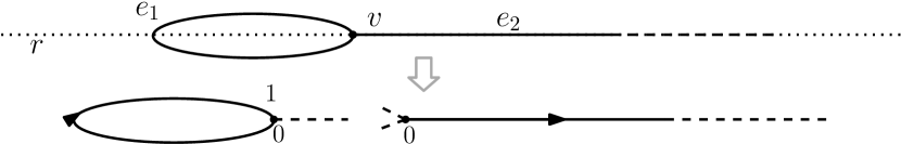
Figure 2. The parametrization of the infinite tadpole graph and its natural symmetry axis $r$.

Let $L^{2}_{p}$ be composed by functions which are periodic on the tail with period $1$, i.e. $L_{2}=1$. We consider the bilinear Schrödinger equation (BSE) in $L^{2}_{p}$ with $A=-\Delta$ the Laplacian equipped with Neumann-Kirchhoff  boundary conditions in the vertex $v$, i.e.

$$\begin{split}D(A)=\Big{\{}\psi=(\psi^{1},\psi^{2})\in H^{2}_{p}\ :\ \psi^{1}(0)=\psi^{1}(1)=\psi^{2}(0),\ \ \ \ \frac{\partial\psi^{1}}{\partial x}(0)-\frac{\partial\psi^{1}}{\partial x}(1)+\frac{\partial\psi^{2}}{\partial x}(0)=0\Big{\}}.\\ \end{split}$$

Remark 3.1.

The chosen operator $A$ is not self-adjoint in the Hilbert space $L^{2}_{p}$. This fact is an important peculiarity of this work with respect to the existing ones on bilinear quantum systems. However, we show how to construct subspaces of $L^{2}_{p}$ composed by eigenspaces of $A$ where the well-posedness and the controllability can be ensured.

We assume the control field $B:\psi=(\psi^{1},\psi^{2})\longmapsto(V^{1}\psi^{1},V^{2}\psi^{2})$ being such that

$$V^{1}(x)=x^{2}(x-1)^{2},\ \ \ \ \ \ \ \ \ \ V^{2}(x)=\sum_{n\in\mathbb{N}}(x-n)^{2}(x-n-1)^{2}\upchi_{[n,n+1]}(x).$$

The choice of the potentials $V_{1}$ and $V_{2}$ is calibrated so that $B$ preserves the space $L^{2}_{p}$ and $V^{1}\psi^{1}\equiv V^{2}\psi^{2}|_{[n,n+1]}$ for every $n\in\mathbb{N}$ when $\psi=(\psi^{1},\psi^{2})\in L^{2}_{p}$ is such that $\psi^{1}\equiv\psi^{2}|_{[n,n+1]}$ for every $n\in\mathbb{N}$. In this framework, the (BSE) corresponds to the two following Cauchy systems respectively in $L^{2}(e_{1},\mathbb{C})$ and $L^{2}_{p}(e_{2},\mathbb{C})$

$$\begin{split}\begin{cases}i\partial_{t}\psi^{1}=-\Delta\psi^{1}+uV^{1}\psi^{1},\\ \psi^{1}(0)=\psi^{1}_{0},\\ \end{cases}\ \ \ \ \ \begin{cases}i\partial_{t}\psi^{2}=-\Delta\psi^{2}+uV^{2}\psi^{2},\\ \psi^{2}(0)=\psi^{2}_{0}.\\ \end{cases}\end{split}$$ (BSEt)

Let $\upvarphi:=\{\varphi_{k}\}_{k\in\mathbb{N}^{*}}$ be an orthonormal system of $L^{2}_{p}$ made by eigenfunctions of $-\Delta$ and corresponding to the eigenvalues $\upmu:=\{\mu_{k}\}_{k\in\mathbb{N}^{*}}$ such that, for every $k\in\mathbb{N}^{*}\setminus\{1\}$,

$$\begin{split}\begin{cases}\varphi_{k}=\big{(}\cos({2(k-1)}\pi x),\cos({2(k-1)}\pi x)\big{)},\ \ \ \ \ \ \ \ \ \ &\mu_{k}={4(k-1)^{2}\pi^{2}},\\ \varphi_{1}=\big{(}\frac{\sqrt{2}}{2},\frac{\sqrt{2}}{2}\big{)},\ \ \ \ \ \ \ \ \ \ &\mu_{1}=0.\end{cases}\end{split}$$

Remark 3.2.

We notice that each $f=(f^{1},f^{2})\in L^{2}_{p}$ belongs to $\mathscr{H}(\upvarphi)$ when

• $f^{1}$ is symmetric with respect to the symmetry axis $r$ of $\mathcal{T}$;

• $f^{2}$ has period $2\pi$ and $f^{2}|_{[2n\pi,2(n+1)\pi]}\equiv f^{1}$ for every $n\in\mathbb{N}$.

Proposition 3.3.

Let $\psi_{0}\in H^{4}_{\mathcal{T}}(\upvarphi)$ and $u\in L^{2}((0,T),\mathbb{R})$. There exists a unique mild solution of the (BSEt) in $H^{4}_{\mathcal{T}}(\upvarphi)$, i.e. a function $\psi\in C^{0}\big{(}[0,T],H^{4}_{\mathcal{T}}(\upvarphi)\big{)}$ such that

$$\psi(t)=e^{i\Delta t}\psi_{0}-i\int_{0}^{t}e^{i\Delta(t-s)}u(s)B\psi(s)ds.\\$$ (5)

Moreover, the flow of (BSEt) on $\mathscr{H}(\upvarphi)$ can be extended to a unitary flow $\Gamma_{t}^{u}$ with respect to the $L^{2}_{p}-$norm such that $\Gamma_{t}^{u}\psi_{0}=\psi(t)$ for any solution $\psi$ of (BSEt) with initial data $\psi_{0}\in\mathscr{H}(\upvarphi)$.

Proof.

1) Unitary flow. We consider Remark 3.2. For every $f=(f^{1},f^{2})\in\mathscr{H}(\upvarphi)$, we notice that $(Bf)^{1}$ inherits from $f^{1}$ the property of being symmetric with respect to the symmetry axis $r$, while $(Bf)^{2}|_{[2n\pi,2(n+1)\pi]}\equiv(Bf)^{1}$ for every $n\in\mathbb{N}$ as $f^{2}|_{[2n\pi,2(n+1)\pi]}\equiv f^{1}$ for every $n\in\mathbb{N}$. Now, $(Bf)^{2}$ has period $2\pi$ and $(Bf)^{2}(x)=(Bf)(2(n+1)\pi-x)$ for every $n\in\mathbb{N}$ and $x\in[2n\pi,(2n+1)\pi].$ Thus, $Bf=(V^{1}f^{1},V^{2}f^{2})\in\mathscr{H}(\upvarphi)$ for every $f=(f^{1},f^{2})\in\mathscr{H}(\upvarphi)$ and the control field $B$ preserves $\mathscr{H}(\upvarphi)$. The space $\mathscr{H}(\upvarphi)$ is a Hilbert space where the operator $A$ is self-adjoint and $B$ is bounded symmetric. Thanks to [6, Theorem 2.5], the (BSEt) admits a unique solution $\psi\in C^{0}([0,T],\mathscr{H}(\upvarphi))$ for every $T>0$ and $\psi_{0}\in\mathscr{H}(\upvarphi)$. The flow of (BSEt) is unitary in $\mathscr{H}(\upvarphi)$ thanks to the following arguments. If $u\in C^{0}((0,T),\mathbb{R})$, then $\psi\in C^{1}((0,T),\mathscr{H}(\upvarphi))$ and $\partial_{t}\|\psi(t)\|_{L^{2}_{p}}^{2}=0$ from (BSEt). Thus $\|\psi(t)\|_{L^{2}_{p}}=\|\psi_{0}\|_{L^{2}_{p}}$. The generalization for $u\in L^{2}((0,T),\mathbb{R})$ follows from a classical density argument, which ensures that the flow of the dynamics of the (BSEt) is unitary in $\mathscr{H}(\upvarphi)$.

2) Regularity of the integral term in the mild solution. The remaining part of the proof refers to the techniques leading to [13, Lemma 1; Proposition 2] (also adopted in the proof of [5, Proposition 2.1]). Let $\psi\in C^{0}([0,T],H_{\mathcal{T}}^{4}(\upvarphi))$ with $T>0$. We notice $B\psi(s)\in H_{p}^{4}\cap H_{\mathcal{T}}^{2}(\upvarphi)$ for almost every $s\in(0,t)$ and $t\in(0,T)$. Let $G(t,x)=\int_{0}^{t}e^{i\Delta(t-s)}u(s)B\psi(s,x)ds$ so that

$$\begin{split}\|G(t)\|_{(4)}&=\Big{(}\sum_{k\in\mathbb{N}^{*}}\Big{|}k^{4}\int_{0}^{t}e^{i\mu_{k}s}\langle\varphi_{k},u(s)B\psi(s,\cdot)\rangle_{L^{2}_{p}}ds\Big{|}^{2}\Big{)}^{\frac{1}{2}}.\\ \end{split}$$

For $f(s,\cdot):=u(s)B\psi(s,\cdot)$ such that $f=(f^{1},f^{2})$ and $k\in\mathbb{N}^{*}\setminus\{1\},$ we have

$$\begin{split}&\langle\varphi_{k},f(s)\rangle_{L^{2}_{p}}=-\frac{1}{\mu_{k}}\Big{(}\int_{0}^{1}\varphi_{k}^{1}(y)\partial_{x}^{2}f^{1}(s,y)dy+\int_{0}^{1}\varphi_{k}^{2}(y)\partial_{x}^{2}f^{2}(s,y)dy\Big{)}\\ &=-\frac{2}{\mu_{k}}\int_{0}^{1}\varphi_{k}^{1}(y)\partial_{x}^{2}f^{1}(s,y)dy=\frac{1}{4(k-1)^{3}\pi^{3}}\int_{0}^{1}\sin(2(k-1)\pi x)\partial_{x}^{3}f^{1}(s,y)dy\\ &=\frac{1}{8(k-1)^{4}\pi^{4}}\Bigg{(}\partial_{x}^{3}f^{1}(s,1)-\partial_{x}^{3}f^{1}(s,0)-\int_{0}^{1}\cos(2(k-1)\pi x)\partial_{x}^{4}f^{1}(s,y)dy\Bigg{)}.\\ \end{split}$$

In the last relations, we considered $\varphi_{k}^{1}(\cdot)\partial_{x}^{2}f^{1}(s,\cdot)|_{[0,1]}=\varphi_{k}^{2}(\cdot)\partial_{x}^{2}f^{2}(s,\cdot)|_{[0,1]}$ as $\partial_{x}^{2}f^{1}(s,\cdot)|_{[0,1]}=\partial_{x}^{2}f^{2}(s,\cdot)|_{[0,1]}$. Equivalently to the first point of the proof of [5, Proposition 2.1], there exists $C_{1}>0$ such that

$$\begin{split}\|G(t)\|_{(4)}\leq&C_{1}\Big{(}\Big{\|}\int_{0}^{t}\big{(}\partial_{x}^{3}f^{1}(s,1)-\partial_{x}^{3}f^{1}(s,0)\big{)}e^{i\mu_{(\cdot)}s}ds\Big{\|}_{\ell^{2}}+\sqrt{t}\|f\|_{L^{2}((0,t),H^{4}_{p})}\Big{)}.\end{split}$$

Thanks [21, Proposition B.6], there exists $C_{2}(t)>0$ uniformly bounded for $t$ in bounded intervals such that $\|G(t)\|_{(4)}\leq C_{2}(t)\|f(\cdot,\cdot)\|_{L^{2}((0,t),H^{4}_{p})}.$ For every $t\in[0,T]$, the last inequality shows that $G(t)\in H^{4}_{\mathcal{T}}(\upvarphi)$ and the provided upper bound is uniform. The Dominated Convergence Theorem leads to $G\in C^{0}([0,T],H^{4}_{\mathcal{T}}(\upvarphi))$.

3) Conclusion. As $Ran(B|_{H_{\mathcal{T}}^{4}}(\upvarphi))\subseteq H_{p}^{4}\cap H^{2}_{\mathcal{T}}(\upvarphi)\subseteq H^{4}_{p}$, we have $B\in\mathcal{L}(H^{4}_{\mathcal{T}}(\upvarphi),H^{4}_{p})$ thanks to the arguments of [24, Remark 2.1]. Let $\psi_{0}\in H^{4}_{\mathcal{T}}(\upvarphi)$. We consider the map

$$F:\psi\in C^{0}([0,T],H^{4}_{\mathcal{T}}(\upvarphi))\mapsto\phi\in C^{0}([0,T],H^{4}_{\mathcal{T}}(\upvarphi)),$$

$$\phi(t)=F(\psi)(t)=e^{i\Delta t}\psi_{0}-\int_{0}^{t}e^{i\Delta(t-s)}u(s)B\psi(s)ds,\ \ \ \ \ \forall t\in[0,T].$$

For every $\psi_{1},\psi_{2}\in C^{0}([0,T],H^{4}_{\mathcal{T}}(\upvarphi))$, from the first point of the proof, there exists $C(t)>0$ uniformly bounded for $t$ lying on bounded intervals such that

$$\begin{split}&\|F(\psi_{1})-F(\psi_{2})\|_{L^{\infty}((0,T),H^{4}_{\mathcal{T}}(\upvarphi))}\leq\left\|\int_{0}^{(\cdot)}e^{i\Delta((\cdot)-s)}u(s)B(\psi_{1}(s)-\psi_{2}(s))ds\right\|_{L^{\infty}((0,T),H^{4}_{\mathcal{T}}(\upvarphi))}\\ &\leq C(T)\|u\|_{L^{2}((0,T),\mathbb{R})}{\,|\kern-1.07639pt|\kern-1.07639pt|\,}B{\,|\kern-1.07639pt|\kern-1.07639pt|\,}_{\mathcal{L}(H^{4}_{\mathcal{T}}(\upvarphi),H^{4}_{p})}\|\psi_{1}-\psi_{2}\|_{L^{\infty}((0,T),H^{4}_{\mathcal{T}}(\upvarphi))}.\\ \end{split}$$

If $\|u\|_{L^{2}((0,T),\mathbb{R})}$ is small enough, then $F$ is a contraction and Banach Fixed Point Theorem yields the existence of $\psi\in C^{0}([0,T],H^{4}_{\mathcal{T}}(\upvarphi))$ such that $F(\psi)=\psi.$ When $\|u\|_{L^{2}((0,T),\mathbb{R})}$ is not sufficiently small, we decompose $(0,T)$ with a sufficiently thin partition $\{t_{j}\}_{0\leq j\leq n}$ with $n\in\mathbb{N}^{*}$ such that each $\|u\|_{L^{2}((t_{j-1},t_{j}),\mathbb{R})}$ is so small such that $F$ defined on the interval $[t_{j-1},t_{j}]$ is a contraction. The well-posedness on $[0,T]$ is defined by gluing each flow defined in every interval of the partition. ∎

We are finally ready to present the following global exact controllability result (Definition 2.1).

Theorem 3.4.

The (BSEt) is globally exactly controllable in $H^{4}_{\mathcal{T}}(\upvarphi)$.

Proof.

The statement is proved by using the arguments adopted in the proof of [5, Theorem 2.2].

1) Local exact controllability. We notice that $\varphi_{1}(T)=e^{-i\mu_{1}T}\varphi_{1}=\varphi_{1}$ with $T>0$ as the first eigenvalue $\mu_{1}$ is equal to $0$. For $\epsilon,T>0$, we define

$$O_{\epsilon}^{4}:=\big{\{}\psi\in H_{\mathcal{T}}^{4}(\upvarphi)\big{|}\ :\ \|\psi\|_{L^{2}_{p}}=1,\ \|\psi-\varphi_{1}\|_{(4)}<\epsilon\big{\}}.$$

We ensure there exist $T,\epsilon>0$ so that, for every $\psi\in O_{\epsilon}^{4}$, there exists $u\in L^{2}((0,T),\mathbb{R})$ such that $\psi=\Gamma^{u}_{T}\varphi_{1}.$ The result can be proved by showing the surjectivity of the map $\Gamma_{T}^{(\cdot)}\varphi_{1}:u\in L^{2}((0,T),\mathbb{R})\longmapsto\psi\in O_{\epsilon}^{4}$ with $T>0$. Let

$$\Gamma_{t}^{(\cdot)}\varphi_{1}=\sum_{k\in\mathbb{N}^{*}}{\varphi_{k}(t)}\langle\varphi_{k}(t),\Gamma_{t}^{(\cdot)}\varphi_{1}\rangle_{L^{2}_{p}}.$$

We recall the definition of $h^{4}$ provided in (4). Let $\alpha$ be the map defined as the sequence with elements $\alpha_{k}(u)=\langle\varphi_{k}(T),\Gamma_{T}^{u}\varphi_{1}\rangle_{L^{2}_{p}}$ for $k\in\mathbb{N}^{*}$ such that

$$\alpha:L^{2}((0,T),\mathbb{R})\longrightarrow Q:=\{{\bf x}:=\{x_{k}\}_{k\in\mathbb{N}^{*}}\in h^{4}(\mathbb{C})\ |\ \|{\bf x}\|_{\ell^{2}}=1\}.$$

The local exact controllability follows from the local surjectivity of $\alpha$ in a neighborhood of $\alpha(0)=\updelta=\{\delta_{k,1}\}_{k\in\mathbb{N}^{*}}$ with respect to the $h^{4}-$norm. To this end, we consider the Generalized Inverse Function Theorem and we study the surjectivity of $\gamma(v):=(d_{u}\alpha(0))\cdot\ v$ the Fréchet derivative of $\alpha$. Let $B_{k,1}:=\langle\varphi_{k},B\varphi_{1}\rangle_{L^{2}_{p}}$ with $k\in\mathbb{N}^{*}$. The map $\gamma$ is the sequence of elements $\gamma_{k}(v):=-i\int_{0}^{T}v(\tau)e^{i(\mu_{k}-\mu_{1})s}d\tau B_{k,1}$ with $k\in\mathbb{N}^{*}$ so that

$$\gamma:L^{2}((0,T),\mathbb{R})\longrightarrow T_{\updelta}Q=\{{\bf x}:=\{x_{k}\}_{k\in\mathbb{N}^{*}}\in h^{4}(\mathbb{C})\ |\ ix_{1}\in\mathbb{R}\}.$$

As $\mu_{1}=0$, the surjectivity of $\gamma$ corresponds to the solvability of the moments problem

$$\begin{split}{x_{k}}{B_{k,1}^{-1}}=-i\int_{0}^{T}u(\tau)e^{i\mu_{k}\tau}d\tau,\ \ \ \ \ \ \ \ \ \ \forall\{x_{k}\}_{k\in\mathbb{N}^{*}}\in T_{\updelta}Q\subset h^{4}.\\ \end{split}$$ (6)

By direct computation, there exists $C>0$ such that $|B_{k,1}|=|\langle\varphi_{k},B\varphi_{1}\rangle_{L^{2}_{p}}|\geq\frac{C}{k^{4}}$ for every $k\in\mathbb{N}^{*}$ and

$$\big{\{}x_{k}B_{k,1}^{-1}\big{\}}_{k\in\mathbb{N}^{*}}\in\ell^{2},\ \ \ \ \ \ \ \ \ \ \ \ \ \ \ i{x_{1}}B_{k,1}^{-1}\in\mathbb{R}.$$

In conclusion, the solvability of $(\ref{mome1})$ is guaranteed by [21, Proposition B.5] since

$$\{ix_{k}B_{k,1}^{-1}\}_{k\in\mathbb{N}^{*}}\in\{\{c_{k}\}_{k\in\mathbb{N}^{*}}\in\ell^{2}\ |\ c_{1}\in\mathbb{R}\},\ \ \ \ \ \ \inf_{k\in\mathbb{N}^{*}}|\mu_{k+1}-\mu_{k}|={4\pi^{2}}.$$

2) Global exact controllability. Let $T,\epsilon>0$ be so that 1) is valid. Thanks to Remark A.3, for any $\psi_{1},\psi_{2}\in H^{4}_{\mathcal{T}}(\upvarphi)$ such that $\|\psi_{1}\|_{L^{2}_{p}}=\|\psi_{2}\|_{L^{2}_{p}}=p$, there exist $T_{1},T_{2}>0$, $u_{1}\in L^{2}((0,T_{1}),\mathbb{R})$ and $u_{2}\in L^{2}((0,T_{2}),\mathbb{R})$ such that

$$\|\Gamma^{u_{1}}_{T_{1}}p^{-1}\psi_{1}-\varphi_{1}\|_{(4)}<{\epsilon},\ \ \ \ \ \|\Gamma^{u_{2}}_{T_{2}}p^{-1}\psi_{2}-\varphi_{1}\|_{(4)}<{\epsilon}$$

and $p^{-1}\Gamma^{u_{1}}_{T_{1}}\psi_{1},p^{-1}\Gamma^{u_{2}}_{T_{2}}\psi_{2}\in O_{\epsilon}^{4}.$ From 1), there exist $u_{3},u_{4}\in L^{2}((0,T),\mathbb{R})$ such that

$$\Gamma_{T}^{u_{3}}\Gamma^{u_{1}}_{T_{1}}\psi_{1}=\Gamma_{T}^{u_{4}}\Gamma^{u_{2}}_{T_{2}}\psi_{2}=p\varphi_{1}\ \ \ \ \Longrightarrow\ \ \ \ \ \exists T>0,\ \widetilde{u}\in L^{2}((0,\widetilde{T}),\mathbb{R})\ \ :\ \ \Gamma_{\widetilde{T}}^{\widetilde{u}}\psi_{1}=\psi_{2}.$$

∎

Let $\Phi:=\{\phi_{k}\}_{k\in\mathbb{N}^{*}}$ be an orthonormal system of $L^{2}_{p}$ made by eigenfunctions of $-\Delta$ and corresponding to the eigenvalues $\Lambda:=\{\lambda_{k}\}_{k\in\mathbb{N}^{*}}$ such that

$$\phi_{k}=\big{(}\sqrt{{2}}\sin({2k}\pi x),0\big{)},\ \ \ \ \ \ \ \ \ \ \lambda_{k}={4k^{2}\pi^{2}},\ \ \ \ \ \ \ \ \ \ \forall k\in\mathbb{N}^{*}.$$

We notice that the results [5, Theorem 2.1; Theorem 2.2] are still valid in the current framework and they lead to the following proposition.

Proposition 3.5.

Let (BSEt) be considered with $V_{1}(x)=x(1-x)$ and $V_{2}=0$ The (BSEt) is well-posed and globally exactly controllable in $H^{3}_{\mathcal{T}}(\Phi)$.

The techniques leading to Proposition 3.3, Theorem 3.4 and Proposition 3.5 also imply the following corollary.

Corollary 3.6.

Let (BSEt) be considered with

$$V^{1}(x)=x(1-x)+x^{2}(x-1)^{2},\ \ \ V^{2}(x)=\sum_{n\in\mathbb{N}}(x-n)^{2}(x-n-1)^{2}\upchi_{[n,n+1]}(x).$$

The (BSEt) is well-posed and globally exactly controllable in $H^{4}_{\mathcal{T}}(\upvarphi)$ and $H^{3}_{\mathcal{T}}(\Phi)$.

Remark 3.7.

The choice of the lengths $L_{1}=1$ and $L_{2}=1$ has been done in order to simplify the theory of the current section. Nevertheless, it is possible to obtain similar results by considering different parameters $L_{1}$ and $L_{2}$ such that $L_{1}/L_{2}\in\mathbb{Q}$. A very similar situation is considered in the next section for a star graph with infinite spokes.

4. Star graph with infinite spokes

Let $\mathscr{S}$ be a star graph composed by $N$ segments $\{e_{j}\}_{1\leq j\leq N}$ of lengths $\{L_{j}\}_{1\leq j\leq N}$ and $\widetilde{N}$ half-lines $\{e_{j}\}_{N+1\leq j\leq N+\widetilde{N}}$. The edges are connected in the internal vertex $v$, while $\{v_{j}\}_{1\leq j\leq N}$ are the external vertices of $\mathscr{S}$ (those vertices of $\mathscr{S}$ connected with only one edge). Each $e_{j}$ with $1\leq j\leq N$ is associated to a coordinate starting from $0$ in $v_{j}$ and going to $L_{j}$, while $e_{j}$ with $N+1\leq j\leq N+\widetilde{N}$ is parametrized with a coordinate starting from $0$ in $v$ and going to infinite.

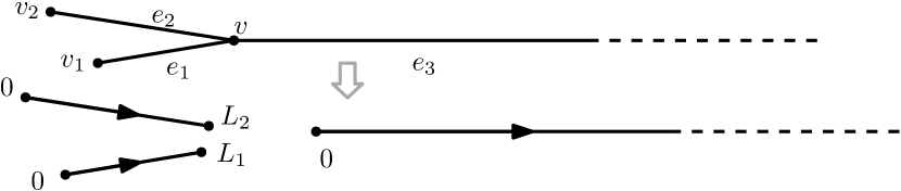
Figure 3. The parametrization of a star graph composed by $N=2$ segments and $\widetilde{N}=1$ half-lines.

Let $L^{2}_{p}$ be defined in (3). This space is composed by functions which are periodic on the infinite edges with periods $\{L_{j}\}_{N+1\leq j\leq N+\widetilde{N}}$. We consider the bilinear Schrödinger equation (BSE) in $L^{2}_{p}$ and the Laplacian $A=-\Delta$ being equipped with Neumann-Kirchhoff  boundary conditions in $v$ and Neumann  boundary conditions in $\{v_{j}\}_{1\leq j\leq N}$, i.e.

$$\begin{split}D(A)=&\Big{\{}\psi=(\psi^{1},...,\psi^{N+\widetilde{N}})\in H^{2}_{p}\ \ :\ \ \sum_{j=1}^{N}\frac{\partial\psi^{j}}{\partial x}(L_{j})=\sum_{j=N+1}^{N+\widetilde{N}}\frac{\partial\psi^{j}}{\partial x}(0),\\ &\ \ \ \psi\in C^{0}(\mathscr{S},\mathbb{C}),\ \ \ \ \ \ \frac{\partial\psi^{j}}{\partial x}(v_{j})=0\ \ \ \ \ \forall 1\leq j\leq N\Big{\}}.\\ \end{split}$$

Let $B:\psi\in L^{2}_{p}\mapsto B\psi=\big{(}(B\psi)^{1},...,(B\psi)^{N+\widetilde{N}}\big{)}$ be a bounded symmetric operator. The (BSE) corresponds to the following Cauchy systems in $L^{2}(e_{j},\mathbb{C})$ when $1\leq j\leq N$ and in $L^{2}_{p}(e_{j},\mathbb{C})$ when $N+1\leq j\leq N+\widetilde{N}$

$$\begin{split}\begin{cases}i\partial_{t}\psi^{j}(t)=-\Delta\psi^{j}(t)+u(t)(B\psi)^{j}(t),&\ \ \ \ \ \ t\in(0,T),\\ \psi^{j}(0)=\psi^{j}_{0}.\\ \end{cases}\end{split}$$ (BSEs)

Remark 4.1.

As in Section 3, the chosen operator $A$ is not self-adjoint in the Hilbert space $L^{2}_{p}$. The central point here is to seek for the correct framework where the existence of eigenfunctions for $A$ is guaranteed. It is clear that the periodicity conditions on each infinite edge $e_{j}$ with $N+1\leq j\leq N+\widetilde{N}$ force any eigenvalue $\lambda$ of $A$ to be of the form $\frac{4k^{2}\pi^{2}}{L_{j}}$ with $k\in\mathbb{N}$. Thus, the eigenvalues $\lambda$ has to be contained in $\bigcap_{N+1\leq j\leq N+\widetilde{N}}\big{\{}\frac{4k^{2}\pi^{2}}{L_{j}}\big{\}}_{k\in\mathbb{N}^{*}}$ which has to be non-empty. This is possible for suitable resonant lengths for the edges of the graphs. In the following part of this section we introduce a set of assumptions ensuring this fact.

Let $L_{N+1}/L_{j}\in\mathbb{Q}$ for every $N+2\leq j\leq N+\widetilde{N}$. We denote by $l_{j}\in\mathbb{N}^{*}$ the smallest natural number such that

$$l_{j}\frac{L_{N+1}}{L_{j}}\in\mathbb{N}^{*},\ \ \ \ \ \ \ \text{with}\ \ \ \ 1\leq j\leq N+\widetilde{N}.$$ (7)

Let $n_{k}:=(k-1)\prod_{j=N+1}^{N+\widetilde{N}}l_{j}\frac{L_{N+1}}{L_{j}}\in\mathbb{N}^{*}$ for every $k\in\mathbb{N}^{*}$. We notice

$$\bigcap_{j=N+1}^{N+\widetilde{N}}\Big{\{}\frac{2m\pi}{L_{j}}\Big{\}}_{m\in\mathbb{N}^{*}}=\Big{\{}\frac{2n_{k}\pi}{L_{N+1}}\Big{\}}_{k\in\mathbb{N}^{*}}.$$

Assumptions A.

The numbers $\{L_{j}\}_{1\leq j\leq N+\widetilde{N}}$ are such that every ratio $\frac{L_{N+1}}{L_{j}}\in\mathbb{Q}$ for any $N+2\leq j\leq N+\widetilde{N}$. In addition, there exist $J\subseteq\mathbb{N}^{*}$ with $|J|=+\infty$ and $\{c_{j}\}_{N+1\leq j\leq N+\widetilde{N}}$ with $c_{j}\in[0,L_{j}]$ for any ${N+1\leq j\leq N+\widetilde{N}}$ such that

$$\sum_{j=1}^{N}\tan\Big{(}\frac{2n_{k}\pi}{L_{N+1}}L_{j}\Big{)}=\sum_{j=N+1}^{N+\widetilde{N}}\tan\Big{(}\frac{2n_{k}\pi}{L_{N+1}}c_{j}\Big{)},\ \ \ \ \ \ \ \ \ \forall k\in J.$$

In conclusion, the sequence $(\mu_{k})_{k\in\mathbb{N}^{*}}=\Big{(}\frac{4n_{k}^{2}\pi^{2}}{L_{N+1}^{2}}\Big{)}_{k\in J}$ is such that $\mu_{k}\sim k^{2}$, i.e. there exist $C_{1},C_{2}>0$ such that

$$C_{1}k^{2}\leq\mu_{k}\leq C_{2}k^{2},\ \ \ \ \ \ \forall k\in\mathbb{N}^{*}.$$

When Assumptions A are satisfied, we define $\{\varphi_{k}\}_{k\in\mathbb{N}^{*}}$ such that

$$\begin{split}\begin{cases}\varphi_{1}^{j}=\frac{1}{\sqrt{{(N+\widetilde{N})L_{j}}}},\ \ \ \ \ &\forall\ 1\leq j\leq N+\widetilde{N},\\ \varphi_{k}^{1}=\alpha_{k}\cos(\sqrt{\mu}_{k}x),\\ \varphi_{k}^{j}=\alpha_{k}\frac{\cos(\sqrt{\mu}_{k}L_{1})}{\cos(\sqrt{\mu}_{k}L_{j})}\cos(\sqrt{\mu}_{k}x),\ \ \ \ \ \ \ \ \ \ \ \ &\forall\ 2\leq j\leq N,\\ \varphi_{k}^{j}=\alpha_{k}\frac{\cos(\sqrt{\mu}_{k}L_{1})}{\cos(\sqrt{\mu}_{k}c_{j})}\cos(\sqrt{\mu}_{k}(x+c_{j})\Big{)},\ \ \ \ \ \ \ \ \ \ \ \ \ \ &\forall\ N+1\leq j\leq N+\widetilde{N}\\ \end{cases}\end{split}$$ (8)

with $\alpha_{k}\in\mathbb{C}$ such that $\|\varphi_{k}\|_{L^{2}_{p}}=1$ and for every $k\in\mathbb{N}^{*}\setminus\{1\}$.

Lemma 4.2.

Let $\mathscr{S}$ be a star graph satisfying Assumptions A. The sequence $\{\varphi_{k}\}_{k\in\mathbb{N}^{*}}$ is an orthonormal system of $L_{p}^{2}$ made by eigenfunctions of the Laplacian $A$ corresponding to the eigenvalues $(\mu_{k})_{k\in\mathbb{N}^{*}}$.

Proof.

We notice that any eigenfunction $f=(f^{1},...,f^{N+\widetilde{N}})$ of $A$ corresponding to an eigenvalue $\mu$ has to be such that $f^{j}$ has period $\frac{2\pi}{L_{j}}$ for every $N+1\leq j\leq N+\widetilde{N}$. Thus,

$$\sqrt{\mu}\in\bigcap_{j=N+1}^{N+\widetilde{N}}\Big{\{}\frac{2m\pi}{L_{j}}\Big{\}}_{m\in\mathbb{N}^{*}}\supseteq\Big{\{}\frac{2n_{k}\pi}{L_{N+1}}\Big{\}}_{k\in J}.$$

Thanks to the Neumann boundary conditions in $\{v_{j}\}_{j\leq N}$ and to the periodicity conditions in $\{e_{j}\}_{N+1\leq j\leq N+\widetilde{N}}$, there exist $c_{j}\in[0,L_{j}]$ for any ${N+1\leq j\leq N+\widetilde{N}}$ such that

$$\begin{split}\begin{cases}f^{j}=\alpha_{j}\cos(\sqrt{\mu}x),\ \ \ \ \ \ \ \ &1\leq j\leq N,\\ f^{j}=\alpha_{j}\cos(\sqrt{\mu}(x+c_{j}))+\beta_{j}\sin(\sqrt{\mu}(x+c_{j})),\ \ \ \ \ \ \ \ \ &N+1\leq j\leq N+\widetilde{N},\\ \end{cases}\end{split}$$

with suitable $\{\alpha_{j}\}_{j\neq N+\widetilde{N}},\{\beta_{j}\}_{N+1\leq j\neq N+\widetilde{N}}\subset\mathbb{C}$. The Neumann-Kirchhoff boundary conditions in $v$ yield

$$\begin{split}\begin{cases}\alpha_{1}\cos(\sqrt{\mu}L_{1})=\alpha_{j}\cos(\sqrt{\mu}L_{j}),\ \ \ \ \ \ \ \ \ &\forall 2\leq j\leq N,\\ \alpha_{1}\cos(\sqrt{\mu}L_{1})=\alpha_{j}\cos(c_{j})+\beta_{j}\sin(c_{j}),\ \ \ \ \ \ \ \ \ &\forall N+1\leq j\leq N+\widetilde{N}.\\ \end{cases}\end{split}$$

When $\beta_{j}=0$ for every $N+1\leq j\leq N+\widetilde{N}$, the last identities implies

$$\begin{split}\begin{cases}f^{1}=\alpha_{j}\cos(\sqrt{\mu}x),\\ f^{j}=\alpha_{j}\frac{\cos(\sqrt{\mu}L_{1})}{\cos(\sqrt{\mu}L_{j})}\cos(\sqrt{\mu}x),\ \ \ \ \ \ \ \ \ \ \ \ &\forall 2\leq j\leq N,\\ f^{j}=\alpha_{j}\frac{\cos(\sqrt{\mu}L_{1})}{\cos(\sqrt{\mu}c_{j})}\cos(\sqrt{\mu}(x+c_{j})),\ \ \ \ \ \ \ \ \ \ \ \ &\forall 2\leq j\leq N.\\ \end{cases}\end{split}$$

We recall that the numbers $c_{j}\in[0,L_{j}]$ for every ${N+1\leq j\leq N+\widetilde{N}}$ are such that

$$\sum_{j=1}^{N}\tan(\sqrt{\mu}L_{j})=\sum_{j=N+1}^{N+\widetilde{N}}\tan(\sqrt{\mu}c_{j}),\ \ \ \ \ \ \ \forall\sqrt{\mu}\in\Big{\{}\frac{2n_{k}\pi}{L_{N+1}}\Big{\}}_{k\in J}.$$

Thus, the second condition characterizing the Neumann-Kirchhoff boundary conditions is verified when $\beta_{j}=0$. As a consequence, $\{\varphi_{k}\}_{k\in\mathbb{N}^{*}}$ is composed by eigenfunctions of $A$. The orthonormality follows from the fact that $\big{\{}\cos\big{(}\frac{2\pi k}{L}x\big{)}\big{\}}_{k\in\mathbb{N}^{*}}$ is an orthogonal family in $L^{2}([0,L],\mathbb{C})$ with $L>0$. ∎

Equivalently to Proposition 3.3, we have the following well-posedness result.

Proposition 4.3.

Let the star graph $\mathscr{S}$ satisfy Assumptions A. Let $B$ be a bounded symmetric operator in $L^{2}_{p}$ such that

$$B:\mathscr{H}(\upvarphi)\longrightarrow\mathscr{H}(\upvarphi),\ \ \ \ \ \ \ \ B:H^{2}_{\mathscr{S}}(\upvarphi)\longrightarrow H^{2}_{\mathscr{S}}(\upvarphi),\ \ \ \ \ \ \ \ B:H_{\mathscr{S}}^{3}(\upvarphi)\longrightarrow H_{p}^{3}\cap H^{2}_{\mathscr{S}}(\upvarphi).$$

Let $\psi_{0}\in H^{3}_{\mathscr{S}}(\upvarphi)$ and $u\in L^{2}((0,T),\mathbb{R})$. There exists a unique mild solution $\psi\in C^{0}([0,T],H^{3}_{\mathscr{S}}(\upvarphi))$ of (BSEs) with initial data $\psi_{0}$. The flow of (BSEs) on $\mathscr{H}(\upvarphi)$ can be extended to a unitary flow $\Gamma_{t}^{u}$ with respect to the $L^{2}_{p}-$norm such that $\Gamma_{t}^{u}\psi_{0}=\psi(t)$ for any solution $\psi$ of (BSEs) with initial data $\psi_{0}\in\mathscr{H}(\upvarphi)$.

Proof.

The proof follows from the same arguments adopted in Proposition 3.3. First, we notice that $A$ is self-adjoint in $\mathscr{H}(\upvarphi)$ and $B$ is bounded symmetric since $B:\mathscr{H}(\upvarphi)\rightarrow\mathscr{H}(\upvarphi)$. Second, we can define an unitary flow for the dynamics of the equation in $\mathscr{H}(\upvarphi)$ as in the proof of the mentioned proposition.

1) Regularity of the integral term in the mild solution. Let $\psi\in C^{0}([0,T],H_{\mathscr{S}}^{3}(\upvarphi))$ with $T>0$. We notice $B\psi(s)\in H^{3}_{p}\cap H_{\mathscr{S}}^{2}(\upvarphi)$ for almost every $s\in(0,t)$ and $t\in(0,T)$. Let $G(t)=\int_{0}^{t}e^{i\Delta(t-s)}u(s)B\psi(s,x)ds$ so that

$$\begin{split}\|G(t)\|_{(3)}&=\Big{(}\sum_{k\in\mathbb{N}^{*}}\Big{|}k^{3}\int_{0}^{t}e^{i\mu_{k}s}\langle\varphi_{k},u(s)B\psi(s,\cdot)\rangle_{L^{2}_{p}}ds\Big{|}^{2}\Big{)}^{\frac{1}{2}}.\\ \end{split}$$

Let $f(s,\cdot):=u(s)B\psi(s,\cdot)$. We define $\partial_{x}f(s)=(\partial_{x}f^{1}(s),...,\partial_{x}f^{N}(s))$ the derivative of $f(s)$. Thanks to the validity of Assumptions A, we have $\sqrt{\mu}_{k}\sim k$ and there exists $C_{1}>0$ such that, for every $k\in\mathbb{N}^{*}\setminus\{1\},$

$$\begin{split}&\left|k^{3}\int_{0}^{t}e^{i\mu_{k}s}\langle\varphi_{k},f(s)\rangle_{L^{2}_{p}}ds\right|\leq\frac{C_{1}}{k}\sum_{j=1}^{N+\widetilde{N}}\left(\left|\partial_{x}\varphi_{k}^{j}(L_{j})\int_{0}^{t}e^{i\mu_{k}s}\partial_{x}^{2}f^{j}(s,L_{j})ds\right|\right.\\ &+\left.\left|\partial_{x}\varphi_{k}^{j}(0)\int_{0}^{t}e^{i\mu_{k}s}\partial_{x}^{2}f^{j}(s,0)ds\right|+\left|\int_{0}^{t}e^{i\mu_{k}s}\int_{0}^{L_{j}}\partial_{x}\varphi_{k}^{j}(y)\partial_{x}^{3}f^{j}(s,y)dyds\right|\right).\\ \end{split}$$

The argument of [5, Remark 3.4] yields that $\partial_{x}^{3}f(s,\cdot)\in\overline{span\big{\{}\mu_{k}^{-1/2}\partial_{x}\varphi_{k}:\ k\in\mathbb{N}^{*}\big{\}}}^{L^{2}}$ for almost every $s\in(0,t)$ and $t\in(0,T)$, and there exists $C_{2}>0$ such that

$$\begin{split}\|G(t)\|_{(3)}\leq&C_{2}\sum_{j=1}^{N+\widetilde{N}}\Big{(}\Big{\|}\int_{0}^{t}\partial_{x}^{2}f^{j}(s,0)e^{i\mu_{(\cdot)}s}ds\Big{\|}_{\ell^{2}}+\Big{\|}\int_{0}^{t}\partial_{x}^{2}f^{j}(s,L_{j})e^{i\mu_{(\cdot)}s}ds\Big{\|}_{\ell^{2}}\Big{)}\\ &+C_{2}\Big{\|}\int_{0}^{t}\big{\langle}{\mu_{(\cdot)}^{-1/2}}\partial_{x}\varphi_{(\cdot)}(s),\partial_{x}^{3}f(s)\big{\rangle}_{L^{2}_{p}}e^{i\mu_{(\cdot)}s}ds\Big{\|}_{\ell^{2}}.\\ \end{split}$$

From [21, Proposition B.6], there exists $C_{3}(t)>0$ uniformly bounded for $t$ in bounded intervals such that $\|G\|_{(3)}\leq C_{3}(t)\|f(\cdot,\cdot)\|_{L^{2}((0,t),H^{3}_{p})}.$ The provided upper bounds are uniform and the Dominated Convergence Theorem leads to $G\in C^{0}([0,T],H^{3}_{\mathscr{S}}(\upvarphi))$.

2) Conclusion. We proceed as in the second point of the proof of Proposition 3.3. Let $\psi_{0}\in H^{3}_{\mathscr{S}}(\upvarphi)$. We consider the map $F:\psi\in C^{0}([0,T],H^{3}_{\mathscr{S}}(\upvarphi))\mapsto\phi\in C^{0}([0,T],H^{3}_{\mathscr{S}}(\upvarphi))$ with

$$\phi(t)=F(\psi)(t)=e^{i\Delta t}\psi_{0}-\int_{0}^{t}e^{i\Delta(t-s)}u(s)B\psi(s)ds,\ \ \ \ \ \forall t\in[0,T].$$

Let $L^{\infty}(H^{3}_{\mathscr{S}}(\upvarphi)):=L^{\infty}((0,T),H^{3}_{\mathscr{S}}(\upvarphi))$. For every $\psi_{1},\psi_{2}\in C^{0}([0,T],H^{3}_{\mathscr{S}}(\upvarphi))$, thanks to 1), there exists $C(t)>0$ uniformly bounded for $t$ lying on bounded intervals such that

$$\begin{split}&\|F(\psi_{1})-F(\psi_{2})\|_{L^{\infty}(H^{3}_{\mathscr{S}}(\upvarphi))}\leq C(T)\|u\|_{L^{2}((0,T),\mathbb{R})}{\,|\kern-1.07639pt|\kern-1.07639pt|\,}B{\,|\kern-1.07639pt|\kern-1.07639pt|\,}_{\mathcal{L}(H^{3}_{\mathscr{S}}(\upvarphi),H_{p}^{3})}\|\psi_{1}-\psi_{2}\|_{L^{\infty}(H^{3}_{\mathscr{S}}(\upvarphi))}.\\ \end{split}$$

The Banach Fixed Point Theorem leads to the claim as in the mentioned proof. ∎

By keeping in mind the definition of global exact controllability provided in Definition 2.1, we present the following result.

Theorem 4.4.

Let the hypotheses of Proposition 4.3 be satisfied. We also assume that

1. there exists $C>0$ such that $|\langle\varphi_{k},B\varphi_{1}\rangle_{L^{2}_{p}}|\geq\frac{C}{k^{3}}$ for every $k\in\mathbb{N}^{*}$;

2. for every $(j,k),(l,m)\in\mathbb{N}^{2}$ such that $(j,k)\neq(l,m)$, $j<k$, $l<m$ and $\mu_{j}-\mu_{k}=\mu_{j}-\mu_{m},$ it holds

   $$\langle\varphi_{j},B\varphi_{j}\rangle_{L^{2}_{p}}-\langle\varphi_{k},B\varphi_{k}\rangle_{L^{2}_{p}}-\langle\varphi_{l},B\varphi_{l}\rangle_{L^{2}_{p}}+\langle\varphi_{m},B\varphi_{m}\rangle_{L^{2}_{p}}\neq 0.$$

The (BSEs) is globally exactly controllable in $H^{3}_{\mathscr{S}}(\upvarphi)$.

Proof.

1) Local exact controllability. The statement follows as Theorem 3.4. First, for $\epsilon,T>0$, the local exact controllability in $O_{\epsilon,T}^{3}:=\big{\{}\psi\in H_{\mathscr{S}}^{3}(\upvarphi)\big{|}\ \|\psi\|_{L^{2}_{p}}=1,\ \|\psi-\varphi_{1}(T)\|_{(3)}<\epsilon\big{\}}$ with $\varphi_{1}(T)=e^{-i\mu_{1}T}\varphi_{1}$ is ensured by proving the surjectivity of the map

$$\gamma:L^{2}((0,T),\mathbb{R})\longrightarrow T_{\updelta}Q=\{{\bf x}:=\{x_{k}\}_{k\in\mathbb{N}^{*}}\in h^{3}(\mathbb{C})\ |\ ix_{1}\in\mathbb{R}\},$$

the sequence of elements $\gamma_{k}(v):=-i\int_{0}^{T}v(\tau)e^{i(\mu_{k}-\mu_{1})s}d\tau B_{k,1}$ with $B_{k,1}:=\langle\varphi_{k},B\varphi_{1}\rangle_{L^{2}_{p}}$ for $k\in\mathbb{N}^{*}$. The surjectivity of $\gamma$ corresponds to the solvability of the moments problem

$$\begin{split}{x_{k}}B_{k,1}^{-1}=-i\int_{0}^{T}u(\tau)e^{i(\mu_{k}-\mu_{1})\tau}d\tau,\ \ \ \ \ \ \ \ \ \ \forall\{x_{k}\}_{k\in\mathbb{N}^{*}}\in T_{\updelta}Q\subset h^{3}.\\ \end{split}$$ (9)

As there exists $C>0$ such that $|\langle\varphi_{k},B\varphi_{1}\rangle_{L^{2}_{p}}|\geq\frac{C}{k^{3}}$ for every $k\in\mathbb{N}^{*}$, we have $\big{\{}x_{k}B_{k,1}^{-1}\big{\}}_{k\in\mathbb{N}^{*}}\in\ell^{2}$ and $i{x_{1}}B_{k,1}^{-1}\in\mathbb{R}.$ The solvability of $(\ref{mome1bis})$ is guaranteed by [21, Proposition B.5] since

$$\inf_{k\in\mathbb{N}^{*}}|\mu_{k+1}-\mu_{k}|\geq{\pi^{2}}\min\{L_{j}^{-2}:\ {N+1\leq j\leq N+\widetilde{N}}\}>0.$$

2) Global exact controllability. The global exact controllability in $H^{3}_{\mathscr{S}}(\upvarphi)$ is ensured as in the second point of the proof of Theorem 3.4 by considering Remark A.4 instead of Remark A.3. ∎

Remark.

Let $\{L_{j}\}_{1\leq j\leq N+\widetilde{N}}$ be such that $\frac{L_{N+1}}{L_{j}}\in\mathbb{Q}\$ for any $1\leq j\leq N+\widetilde{N}$. We notice that Assumptions A are satisfied with $c_{j}=0$ for every $N+1\leq j\leq N+\widetilde{N}$. Indeed, let $l_{j}$ be the numbers defined in (7). The sequence

$$(\mu_{k})_{k\in\mathbb{N}^{*}}:=\Big{\{}\frac{4\widetilde{n}_{k}^{2}\pi^{2}}{L_{N+1}^{2}}\Big{\}}_{k\in\mathbb{N}^{*}}\ \ \ \ \ \ \text{with }\ \ \ \ \widetilde{n}_{k}:=(k-1)\prod_{j=1}^{N+\widetilde{N}}l_{j}\frac{L_{N+1}}{L_{j}}$$

is composed by eigenvalues. The corresponding eigenfunctions $(\varphi_{k})_{k\in\mathbb{N}^{*}}$ are provided in (8). In this framework,

$$\mu_{k}\sim k^{2},\ \ \ \ \ \ \ \tan(\mu_{k}L_{j})=0\ \ \ \ \ \ \ \ \forall k\in\mathbb{N}^{*},\ \ \ 1\leq j\leq N.$$

Thus, the validity of Assumptions A is ensured with $c_{j}=0$ for every $N+1\leq j\leq N+\widetilde{N}$.

Remark.

Let $\mathscr{S}$ satisfy Assumptions A. We consider $\{L_{j}\}_{1\leq j\leq N+\widetilde{N}}$ being such that $\frac{L_{N+1}}{L_{j}}\in\mathbb{Q}\$ for any $1\leq j\leq N+\widetilde{N}$ so that the previous remark is verified. Let $\widetilde{B}:\psi\longmapsto(V^{1}\psi^{1},...,V^{N+\widetilde{N}}\psi^{N+\widetilde{N}})$ be such that

$$\begin{split}\begin{cases}V^{j}(x)=x^{2}(x-L_{j})^{2},\ \ \ \ \ &\forall 1\leq j\leq N,\\ V^{j}(x)=\sum_{n\in\mathbb{N}}(x-nL_{j})^{2}(x-(n+1)L_{j})^{2}\upchi_{[nL_{j},(n+1)L_{j}]}(x),&\forall N+1\leq j\leq N+\widetilde{N}.\end{cases}\end{split}$$

If we consider the operator $B$ on $L^{2}_{p}$ such that $B\psi=\sum_{j=1}^{+\infty}\varphi_{j}\langle\varphi_{j},\widetilde{B}\psi\rangle_{L_{p}^{2}},$ then the corresponding (BSEs) is well-posed and globally exactly controllable in the space $H^{4}_{\mathscr{S}}(\upvarphi)$. The result is proved by using the techniques leading to Proposition 3.3, Proposition 4.3, Theorem 3.4 and Theorem 4.4. In the next section, we ensure in the same way the well-posedness and the global exact controllability in $H^{s}_{\mathscr{G}}$ for suitable $s\geq 3$ with abstract $\mathscr{G}$ and $B$.

5. Generic graphs

In this section, we study the controllability of the (BSE) for a general graph $\mathscr{G}$ made by $N$ finite edges $\{e_{j}\}_{1\leq j\leq N}$ of lengths $\{L_{j}\}_{1\leq j\leq N}$, $\widetilde{N}$ half-lines $\{e_{j}\}_{N+1\leq j\leq N+\widetilde{N}}$ and $M$ vertices $\{v_{j}\}_{1\leq j\leq M}$. For every vertex $v$, we denote $N(v):=\big{\{}l\in\{1,...,N\}\ |\ v\in e_{l}\big{\}}$. We respectively call $V_{e}$ and $V_{i}$ the external and the internal vertices of $\mathscr{G}$, i.e.

$$V_{e}:=\big{\{}v\in\{v_{j}\}_{1\leq j\leq M}\ |\ \exists!e\in\{e_{j}\}_{1\leq j\leq N}:v\in e\big{\}},\ \ \ \ \ V_{i}:=\{v_{j}\}_{1\leq j\leq M}\setminus V_{e}.$$

We consider the bilinear Schrödinger equation (BSE) in $L^{2}_{p}$ for a general graph $\mathscr{G}$. The Laplacian $A=-\Delta$ is equipped with Dirichlet or Neumann boundary conditions in the external vertices, and the internal vertices are equipped with Neumann-Kirchhoff boundary conditions. More precisely, a vertex $v\in V_{i}$ is said to be equipped with Neumann-Kirchhoff boundary conditions when every function $f=(f^{1},...,f^{N})\in D(A)$ is continuous in $v$ and

$$\begin{split}\sum_{l\in N(v)}\frac{\partial f^{l}}{\partial x}(v)=0,\end{split}$$

when the derivatives are assumed to be taken in the directions away from the vertex. We respectively call ($\mathcal{D}$), ($\mathcal{N}$) and ($\mathcal{N}\mathcal{K}$) the Dirichlet, Neumann and Neumann-Kirchhoff boundary conditions characterizing $D(A)$.

We say that a vertex $v$ of $\mathscr{G}$ is equipped with one of the previous boundaries, when each $f\in D(A)$ satisfies it in $v$. We say that $\mathscr{G}$ is equipped with ($\mathcal{D}$) (or ($\mathcal{N}$)) when, for every $f\in D(A)$, the function $f$ satisfies ($\mathcal{D}$) (or ($\mathcal{N}$)) in every $v\in V_{e}$ and verifies ($\mathcal{N}\mathcal{K}$) in every $v\in V_{i}$. In addition, the graph $\mathscr{G}$ is said to be equipped with ($\mathcal{D}$/$\mathcal{N}$) when, for every $f\in D(A)$ and $v\in V_{e}$, the function $f$ satisfies ($\mathcal{D}$) or ($\mathcal{N}$) in $v$, and $f$ verifies ($\mathcal{N}\mathcal{K}$) in every $v\in V_{i}$.

Let $\upvarphi:=\{\varphi_{k}\}_{k\in\mathbb{N}^{*}}$ be an orthonormal system of $L^{2}_{p}$ made by some eigenfunctions of $A$ and let $\{\mu_{k}\}_{k\in\mathbb{N}^{*}}$ be the corresponding eigenvalues. Let $[r]$ be the entire part of $r\in\mathbb{R}$. We define $\mathscr{G}(\upvarphi)=\bigcup_{k\in\mathbb{N}^{*}}supp(\varphi_{k})$ and we respectively denote by $V_{e}(\upvarphi)$ and $V_{i}(\upvarphi)$ the external and internal vertices of $\mathscr{G}(\upvarphi)$. For $s>0$, we introduce the space

$$\begin{split}H^{s}_{\mathcal{N}\mathcal{K}}(\upvarphi):=\Big{\{}&\psi\in\mathscr{H}(\upvarphi)\cap H^{s}_{p}\ |\ \partial_{x}^{2n}\psi\text{ is continuous in }v,\ \forall n\in\mathbb{N},\ n<\big{[}({s+1})/{2}\big{]},\ \forall v\in V_{i};\\ &\sum_{j\in N(v)}\partial_{x}^{2n+1}\psi^{j}(v)=0,\ \forall n\in\mathbb{N},\ n<\big{[}{s}/{2}\big{]},\ \forall v\in V_{i}\Big{\}}.\\ \end{split}$$

Remark 5.1.

We notice the following facts.

• $\mathscr{G}(\upvarphi)$ is a finite or infinite sub-graph of $\mathscr{G}$ whose structure depends on the orthonormal family $\upvarphi$.

• The functions belonging to $\mathscr{H}(\upvarphi)$, $H^{s}_{\mathscr{G}}(\upvarphi)$ and $H^{s}_{\mathcal{N}\mathcal{K}}(\upvarphi)$ can be considered as functions with domain $\mathscr{G}(\upvarphi)$.

• $\mathscr{G}(\upvarphi)$ shares some external and internal vertices with $\mathscr{G}$. Its new external vertices are $V_{e}(\upvarphi)\setminus V_{e}$.

• Let $L^{2}_{p}(\mathscr{G}(\upvarphi),\mathbb{C})$ be the space defined from the identities (3) by considering the graph $\mathscr{G}(\upvarphi)$. Each $\varphi_{k}|_{\mathscr{G}(\upvarphi)}$ is an eigenfunction of a Laplacian $\widetilde{A}$ defined on $L^{2}_{p}(\mathscr{G}(\upvarphi),\mathbb{C})$ as follows. The domain $D(\widetilde{A})$ is composed by the restriction in $\mathscr{G}(\upvarphi)$ of those $H^{2}_{p}$ functions satisfying $(\mathcal{D})$ in the vertices $V_{e}(\upvarphi)\setminus V_{e}$ and verifying the same boundary conditions defining $D(A)$ in the vertices $V_{i}(\upvarphi)\cup\big{(}V_{e}(\upvarphi)\cap V_{e}\big{)}$.

From now on, when we claim that the vertices of $\mathscr{G}(\upvarphi)$ are equipped with any type of boundary conditions, this is done in the meaning of Remark 5.1. Let $\eta>0,$ $a\geq 0$ and

$$I:=\{(j,k)\in(\mathbb{N}^{*})^{2}:j<k\}.$$

Assumptions I ($\upvarphi,\eta$).

Let $B$ be a bounded and symmetric operator in $L^{2}_{p}$ satisfying the following conditions.

1. There exists $C>0$ such that $|\langle\varphi_{k},B\varphi_{1}\rangle_{L^{2}_{p}}|\geq\frac{C}{k^{2+\eta}}$ for every $k\in\mathbb{N}^{*}$.

2. For every $(j,k),(l,m)\in I$ such that $(j,k)\neq(l,m)$ and $\mu_{j}-\mu_{k}=\mu_{j}-\mu_{m},$ it holds $\langle\varphi_{j},B\varphi_{j}\rangle_{L^{2}_{p}}-\langle\varphi_{k},B\varphi_{k}\rangle_{L^{2}_{p}}-\langle\varphi_{j},B\varphi_{j}\rangle_{L^{2}_{p}}+\langle\varphi_{m},B\varphi_{m}\rangle_{L^{2}_{p}}\neq 0.$

Assumptions II ($\upvarphi,\eta,a$).

We have $B:\mathscr{H}(\upvarphi)\rightarrow\mathscr{H}(\upvarphi)$ and $Ran(B|_{H^{2}_{\mathscr{G}}(\upvarphi)})\subseteq H^{2}_{\mathscr{G}}(\upvarphi).$ In addition, one of the following points is satisfied.

1. When $\mathscr{G}(\upvarphi)$ is equipped with ($\mathcal{D}$/$\mathcal{N}$) and $a+\eta\in(0,3/2)$, there exists $d\in[\max\{a+\eta,1\},3/2)$ such that

   $$Ran(B|_{H_{\mathscr{G}}^{2+d}(\upvarphi)})\subseteq H^{2+d}_{p}\cap H^{2}_{\mathscr{G}}(\upvarphi).$$

2. When $\mathscr{G}(\upvarphi)$ is equipped with ($\mathcal{N}$) and $a+\eta\in(0,7/2)$, there exist $d\in[\max\{a+\eta,2\},7/2)$ and $d_{1}\in(d,7/2)$ such that

   $$Ran(B|_{H^{d_{1}}_{\mathcal{N}\mathcal{K}}(\upvarphi)})\subseteq H^{d_{1}}_{\mathcal{N}\mathcal{K}}(\upvarphi),\ \ \ \ \ Ran(B|_{H_{\mathscr{G}}^{2+d}(\upvarphi)})\subseteq H^{2+d}_{p}\cap H^{1+d}_{\mathcal{N}\mathcal{K}}(\upvarphi)\cap H^{2}_{\mathscr{G}}(\upvarphi).$$

3. When $\mathscr{G}$ is equipped with ($\mathcal{D}$) and $a+\eta\in(0,5/2)$, there exists $d\in[\max\{a+\eta,1\},5/2)$ such that

   $$Ran(B|_{H_{\mathscr{G}}^{2+d}(\upvarphi)})\subseteq H^{2+d}_{p}\cap H^{1+d}_{\mathcal{N}\mathcal{K}}(\upvarphi)\cap H^{2}_{\mathscr{G}}(\upvarphi).$$

   If $d\geq 2$, then there exists $d_{1}\in(d,5/2)$ such that $Ran(B|_{H^{d_{1}}_{p}\cap\mathscr{H}(\upvarphi)})\subseteq H^{d_{1}}_{p}\cap\mathscr{H}(\upvarphi).$

From now on, we omit the terms $\upvarphi,$ $\eta$ and $a$ from the notations of Assumptions I and Assumptions II when their are not relevant.

We are finally ready to present some interpolation properties for the spaces $H^{s}_{\mathscr{G}}(\upvarphi)$ with $s>0$.

Proposition 5.2.

Let $\upvarphi:=\{\varphi_{k}\}_{k\in\mathbb{N}^{*}}$ be an orthonormal system of $L^{2}_{p}$ made by eigenfunctions of $A$.

1) If the graph $\mathscr{G}(\upvarphi)$ is equipped with ($\mathcal{D}$/$\mathcal{N}$), then

$$H^{s_{1}+s_{2}}_{\mathscr{G}}(\upvarphi)=H_{\mathscr{G}}^{s_{1}}(\upvarphi)\cap H^{s_{1}+s_{2}}_{p}\ \ \ \text{for}\ \ \ s_{1}\in\mathbb{N},\ s_{2}\in[0,1/2).$$

2) If the graph $\mathscr{G}(\upvarphi)$ is equipped with ($\mathcal{N}$), then

$$H^{s_{1}+s_{2}}_{\mathscr{G}}(\upvarphi)=H_{\mathscr{G}}^{s_{1}}(\upvarphi)\cap H^{s_{1}+s_{2}}_{\mathcal{N}\mathcal{K}}(\upvarphi)\ \ \ \text{for}\ \ \ s_{1}\in 2\mathbb{N}\,\ s_{2}\in[0,3/2).$$

3) If the graph $\mathscr{G}(\upvarphi)$ is equipped with ($\mathcal{D}$), then

$$H^{s_{1}+s_{2}+1}_{\mathscr{G}}(\upvarphi)=H_{\mathscr{G}}^{s_{1}+1}(\upvarphi)\cap H^{s_{1}+s_{2}+1}_{\mathcal{N}\mathcal{K}}(\upvarphi)\ \ \ \text{for}\ \ \ s_{1}\in 2\mathbb{N},\ s_{2}\in[0,3/2).$$

Proof.

Let us start by considering the first point of the statement. We denote by $\{e_{j}\}_{j\leq N_{1}}$ the finite edges composing $\mathscr{G}(\upvarphi)$, while $\{e_{j}\}_{N_{1}+1\leq j\leq N_{1}+\widetilde{N}_{1}}$ are its infinite edges corresponding to the periods $\{L_{j}\}_{N_{1}+1\leq j\leq N_{1}+\widetilde{N}_{1}}$. We define a compact graph $\widetilde{\mathscr{G}}(\upvarphi)$ from $\mathscr{G}(\upvarphi)$ as follows (see Figure 4 for further details). For every $N_{1}+1\leq j\leq N_{1}+\widetilde{N}_{1}$, we cut the edge $e_{j}$ at distance $L_{j}$ from the internal vertex of $\mathscr{G}(\upvarphi)$ where $e_{j}$ is connected. As $\widetilde{\mathscr{G}}(\upvarphi)$ is a compact graph, the space $L^{2}_{p}(\widetilde{\mathscr{G}}(\upvarphi),\mathbb{C})$ corresponds to $L^{2}(\widetilde{\mathscr{G}}(\upvarphi),\mathbb{C})$. There, we consider a self-adjoint Laplacian $\widetilde{A}$ being defined as follows. Every internal vertex of $\widetilde{\mathscr{G}}(\upvarphi)$ is equipped with Neumann-Kirchhoff boundary conditions. Every external vertex of $\widetilde{\mathscr{G}}(\upvarphi)$ belonging to $V_{e}(\upvarphi)$ is equipped with the same boundary conditions of $\mathscr{G}(\upvarphi)$, while every other external vertex is equipped with ($\mathcal{D}$). Finally, we denote by $H^{s}_{\widetilde{\mathscr{G}}(\upvarphi)}:=D(|\widetilde{A}|^{\frac{s}{2}})$ for every $s>0$.

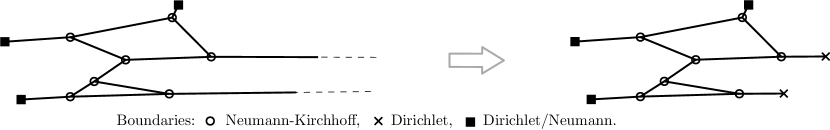
Figure 4. The figure represents an example of definition of the compact graph $\widetilde{\mathscr{G}}(\upvarphi)$ (on the right) from a specific infinite graph $\mathscr{G}(\upvarphi)$ (on the left) composed by $N_{1}=11$ finite edges and $\widetilde{N}_{1}=2$ infinite edges. We also underline the boundary conditions characterizing $D(\widetilde{A})$ in $\widetilde{\mathscr{G}}(\upvarphi)$.

Afterwards, for every edge $e_{j}$ with $N_{1}+1\leq j\leq N_{1}+\widetilde{N}_{1}$, we define a ring $\widetilde{e}_{j}$ having length $L_{j}$. We consider on $L^{2}(\widetilde{e}_{j},\mathbb{C})$ a self-adjoint Laplacian $A_{j}$ with domain $D(A_{j})=H^{2}(\widetilde{e}_{j},\mathbb{C})$ and we denote by $H^{s}_{\widetilde{e}_{j}}:=D(|A_{j}|^{\frac{s}{2}})$ for every $s>0.$ On $L^{2}((0,L_{j}),\mathbb{C})$ with $N_{1}+1\leq j\leq N_{1}+\widetilde{N}_{1}$, we consider a Dirichlet Laplacian $A^{\mathcal{D}}_{j}$ and Neumann Laplacian $A^{\mathcal{N}}_{j}$, while we call, for every $s>0$,

$$H^{s}_{e_{j}^{\mathcal{D}}}:=D(|A^{\mathcal{D}}_{j}|^{\frac{s}{2}}),\ \ \ \ \ \ \ \ \ \ \ \ H^{s}_{e_{j}^{\mathcal{N}}}:=D(|A^{\mathcal{N}}_{j}|^{\frac{s}{2}}).$$

Now, for every $\psi=(\psi^{1},...,\psi^{N_{1}+\widetilde{N}_{1}})\in H^{s_{1}+s_{2}}_{\mathscr{G}}(\upvarphi)$ with $s_{1}\in\mathbb{N}$ and $s_{2}\in[0,1/2)$, there exist

$$\begin{split}\begin{cases}\psi_{1}=(\psi_{1}^{1},...,\psi_{1}^{N_{1}+\widetilde{N}_{1}})\in H^{s_{1}+s_{2}}_{\widetilde{\mathscr{G}}(\upvarphi)},\ \ \ \ \ \ \ \\ f^{j}\in H^{s_{1}+s_{2}}_{\widetilde{e}_{j}},\ \ \ &\forall N_{1}+1\leq j\leq N_{1}+\widetilde{N}_{1},\\ g^{j}\in H^{s_{1}+s_{2}}_{e_{j}^{\mathcal{D}}},\ \ \ &\forall N_{1}+1\leq j\leq N_{1}+\widetilde{N}_{1},\\ h^{j}\in H^{s_{1}+s_{2}}_{e_{j}^{\mathcal{N}}},\ \ \ &\forall N_{1}+1\leq j\leq N_{1}+\widetilde{N}_{1},\end{cases}\end{split}$$

$$\begin{split}\text{such that}\ \ \begin{cases}\psi^{j}\equiv\psi^{j}_{1},\ \ \ \ \ &\forall 1\leq j\leq N_{1},\\ \psi^{j}(x)=\psi^{j}_{1}(x)+g^{j}(x)+h^{j}(x),\ \ \ \ &\forall x\in(0,L_{j}),\ \ \ N_{1}+1\leq j\leq N_{1}+\widetilde{N}_{1},\\ \psi^{j}(x)=f^{j}\big{(}x-\big{[}\frac{x}{L_{j}}\big{]}\big{)},\ \ \ \ &\forall x\in(L_{j},+\infty),\ \ \ N_{1}+1\leq j\leq N_{1}+\widetilde{N}_{1}.\\ \end{cases}\end{split}$$

The last decomposition yields that $H^{s_{1}+s_{2}}_{\mathscr{G}}(\upvarphi)$ can be identified with a suitable subspace of

$$H^{s_{1}+s_{2}}_{\widetilde{\mathscr{G}}(\upvarphi)}\times\prod_{j=N_{1}+1}^{N_{1}+\widetilde{N}_{1}}\big{(}H^{s_{1}+s_{2}}_{\widetilde{e}_{j}}\times H^{s_{1}+s_{2}}_{e_{j}^{\mathcal{D}}}\times H^{s_{1}+s_{2}}_{e_{j}^{\mathcal{N}}}\big{)}.$$

Thanks to the first point of [21, Proposition 4.2], we have

$$\begin{split}\begin{cases}H^{s_{1}+s_{2}}_{\widetilde{\mathscr{G}}(\upvarphi)}=H^{s_{1}}_{\widetilde{\mathscr{G}}(\upvarphi)}\cap H^{s_{1}+s_{2}}(\widetilde{\mathscr{G}}(\upvarphi),\mathbb{C}),\\ H^{s_{1}+s_{2}}_{\widetilde{e}_{j}}=H^{s_{1}}_{\widetilde{e}_{j}}\cap H^{s_{1}+s_{2}}(\widetilde{e}_{j},\mathbb{C}),\ \ \ \ \ \ \ &\forall N_{1}+1\leq j\leq N_{1}+\widetilde{N}_{1},\\ H^{s_{1}+s_{2}}_{e_{j}^{\mathcal{D}}}=H^{s_{1}}_{e_{j}^{\mathcal{D}}}\cap H^{s_{1}+s_{2}}((0,L_{j}),\mathbb{C}),\ \ \ \ \ \ \ &\forall N_{1}+1\leq j\leq N_{1}+\widetilde{N}_{1},\\ H^{s_{1}+s_{2}}_{e_{j}^{\mathcal{N}}}=H^{s_{1}}_{e_{j}^{\mathcal{N}}}\cap H^{s_{1}+s_{2}}((0,L_{j}),\mathbb{C}),\ \ \ \ \ \ \ &\forall N_{1}+1\leq j\leq N_{1}+\widetilde{N}_{1}.\\ \end{cases}\end{split}$$

The last relations imply that, for every $\psi\in H^{s_{1}+s_{2}}_{\mathscr{G}}(\upvarphi)$ with $s_{1}\in\mathbb{N}$ and $s_{2}\in[0,1/2)$, there holds $\psi\in H^{s_{1}}_{\mathscr{G}}(\upvarphi)\cap H^{s_{1}+s_{2}}_{p}$ achieving the proof of the first point of the proposition. The second and the third statement follow from the same techniques by respectively using the second and third point of [21, Proposition 4.2].∎

In the following theorem, we collect the well-posedness and the controllability result for the bilinear Schrödinger equation in this general framework. The well-posedness is proved exactly as [5, Proposition 3.3] by using Proposition 5.2 instead of [5, Proposition 3.2]. The controllability result subsequently follows from the same arguments of [5, Theorem 3.6] by considering Proposition A.2 instead of [5, Proposition B.2].

Theorem 5.3.

Let $\upvarphi:=\{\varphi_{k}\}_{k\in\mathbb{N}^{*}}$ be an orthonormal system of $L^{2}_{p}$ made by some eigenfunctions of $A$ and let $\{\mu_{k}\}_{k\in\mathbb{N}^{*}}$ be the corresponding eigenvalues.

1) Let the couple $(A,B)$ satisfy Assumptions II$(\upvarphi,\eta,\tilde{d})$ with $\eta>0$ and $\tilde{d}\geq 0$. Let $d$ be introduced in Assumptions II and $\mu_{k}\sim k^{2}$. For every $\psi_{0}\in H^{2+d}_{\mathscr{G}}(\upvarphi)$ and $u\in L^{2}((0,T),\mathbb{R})$ with $T>0$. There exists a unique mild solution $\psi\in C_{0}([0,T],H^{s}_{\mathscr{G}}(\upvarphi))$ of the (BSE). In addition, the flow of (BSE) on $\mathscr{H}(\upvarphi)$ can be extended to a unitary flow $\Gamma_{t}^{u}$ with respect to the $L^{2}_{p}-$norm such that $\Gamma_{t}^{u}\psi_{0}=\psi(t)$ for any solution $\psi$ of (BSE) with initial data $\psi_{0}\in\mathscr{H}(\upvarphi)$.

2) If there exist $C>0$ and $\tilde{d}\geq 0$ such that

$$|\mu_{k+1}-\mu_{k}|\geq Ck^{-{\tilde{d}}},\ \ \ \ \ \ \ \ \ \ \ \ \forall k\in\mathbb{N}^{*}$$

and if $(A,B)$ satisfies Assumptions I$(\upvarphi,\eta)$ and Assumptions II$(\upvarphi,\eta,\tilde{d})$ for $\eta>0$, then the (BSE) is globally exactly controllable in $H^{s}_{\mathscr{G}}(\upvarphi)$ for $s=2+d$ with $d$ from Assumptions II.

Acknowledgments. The second author was financially supported by the ISDEEC project by ANR-16-CE40-0013.

Appendix A Global approximate controllability

Let us denote by $U(\mathscr{H})$ the space of the unitary operators on a Hilbert space $\mathscr{H}.$

Definition A.1.

Let $\upvarphi:=\{\varphi_{k}\}_{k\in\mathbb{N}^{*}}$ be an orthonormal system of $L^{2}_{p}$ made by some eigenfunctions of $A$. The (BSE) is said to be globally approximately controllable in $H_{\mathscr{G}}^{s}(\upvarphi)$ with $s>0$ if the following assertion is verified. For every $\epsilon>0$, $\psi\in H^{s}_{\mathscr{G}}(\upvarphi)$ and $\widehat{\Gamma}\in U(\mathscr{H}(\upvarphi))$ such that $\widehat{\Gamma}\psi\in H^{s}_{\mathscr{G}}(\upvarphi)$, there exist $T>0$ and $u\in L^{2}((0,T),\mathbb{R})$ such that

$$\|\widehat{\Gamma}\psi-\Gamma^{u}_{T}\psi\|_{(s)}<\epsilon.$$

Proposition A.2.

Let $\upvarphi:=\{\varphi_{k}\}_{k\in\mathbb{N}^{*}}$ be an orthonormal system of $L^{2}_{p}$ made by some eigenfunctions of $A$. If the hypotheses of Theorem 5.3 are satisfied, then the (BSE) is globally approximately controllable in $H^{s}_{\mathscr{G}}(\upvarphi)$ for $s=2+d$ with $d$ from Assumptions II.

Proof.

The proof is the same of [5, Proposition B.2].∎

Remark A.3.

Let us consider the framework introduced in Section 3 with $\mathcal{T}$ an infinite tadpole graph. As Proposition A.2, the problem (BSEt) is globally approximately controllable in $H_{\mathcal{T}}^{4}(\upvarphi)$ when the hypotheses of Theorem 3.4 are verified. Indeed, for every $(j,k),(l,m)\in\{(j,k)\in(\mathbb{N}^{*})^{2}:j<k\}$ so that $(j,k)\neq(l,m)$ and such that $\mu_{j}-\mu_{k}-\mu_{j}+\mu_{m}={\pi^{2}}(j^{2}-k^{2}-l^{2}+m^{2})=0,$ there exists $C>0$ such that

$$\begin{split}&\langle\varphi_{j},B\varphi_{j}\rangle_{L^{2}_{p}}-\langle\varphi_{k},B\varphi_{k}\rangle_{L^{2}_{p}}-\langle\varphi_{l},B\varphi_{l}\rangle_{L^{2}_{p}}+\langle\varphi_{m},B\varphi_{m}\rangle_{L^{2}_{p}}=C(j^{-4}-k^{-4}-l^{-4}+m^{4})\neq 0.\end{split}$$

Finally, the arguments leading to Proposition A.2 also ensure the claim.

Remark A.4.

Let us consider the framework introduced in Section 4 with $\mathscr{S}$ a star graph composed by a finite number of edges of finite or infinite length. Equivalently to Remark A.3, the (BSEs) is globally approximately controllable in $H_{\mathscr{S}}^{3}(\upvarphi)$ when the hypotheses of Theorem 4.4 are verified. Indeed, for every $(j,k),(l,m)\in\{(j,k)\in(\mathbb{N}^{*})^{2}:j<k\}$ so that $(j,k)\neq(l,m)$ and such that $\mu_{j}-\mu_{k}-\mu_{j}+\mu_{m}=0,$ we have

$$\begin{split}&\langle\varphi_{j},B\varphi_{j}\rangle_{L^{2}_{p}}-\langle\varphi_{k},B\varphi_{k}\rangle_{L^{2}_{p}}-\langle\varphi_{j},B\varphi_{j}\rangle_{L^{2}_{p}}+\langle\varphi_{m},B\varphi_{m}\rangle_{L^{2}_{p}}\neq 0.\end{split}$$

Data availability. Data sharing is not applicable to this article as no new data were created or analyzed in this study.

References

[1]
S. Alexander, “Superconductivity of networks. a percolation approach to the effects
of disorder”, Phys. Rev. B 27 (3), 1541–1557 (1983).
[2]
F. Ali Mehmeti, K. Ammari and S. Nicaise, “Dispersive effects for the Schrödinger equation on a tadpole
graph”, Journal of Mathematical Analysis and Applications 448 (1), 262–280 (2017).
[3]
F. Ali Mehmeti, K. Ammari and S. Nicaise, “Dispersive effects and high frequency behaviour for the Schrödinger
equation in star-shaped networks”, Port. Math. 72 (4), 309–355 (2015).
[4]
C. Altafini, “Controllability of quantum mechanical systems by root space decomposition”, J. Math.
Phys. 43 (5), 2051–2062 (2002).
[5]
K. Ammari and A. Duca, “Controllability of localized quantum states on infinite graphs through
bilinear control fields”, International
Journal of Control (2019)
[6]
J. M. Ball, J. E. Marsden, and M. Slemrod, “Controllability for distributed bilinear systems”, SIAM J. Control
Optim. 20 (4), 575–597 (1982).
[7] J. M. Ball and M. Slemrod, “Feedback stabilization of distributed semilinear control systems”,
Appl. Math. Opt. 5 (1), 169–179 (1979).
[8] J. M. Ball, “On the asymptotic behaviour of generalized processes, with applications to nonlinear
evolution equations”, J. Differential Equations. 27 (2), 224–265 (1978).
[9]
C. Bardos, G. Lebeau, and J. Rauch, “Sharp sufficient conditions for the observation, control, and
stabilization of waves from the boundary”, SIAM J. Control Optim. 30 (5), 1024–1065 (1992).
[10]
L. Baudouin and A. Mercado, “An inverse problem for Schrödinger equations with discontinuous
main coefficient”, Appl. Anal. 87 (10-11), 1145–1165 (2008).
[11]
K. Beauchard, “Local controllability of a 1-D Schrödinger equation”, J. Math. Pures Appl. (9) 84 (7), 851–956 (2005).
[12]
K. Beauchard and C. Laurent,
“Bilinear control of high frequencies for a 1D Schrödinger
equation”, Mathematics of Control, Signals, and Systems 29 (2), (2017).
[13]
K. Beauchard and C. Laurent, “Local controllability of 1D linear and nonlinear Schrödinger
equations with bilinear control”, J. Math. Pures Appl. (9) 94 (5), 520–554 (2010).
[14]
U. Boscain, M. Caponigro, and M. Sigalotti, “Multi-input Schrödinger equation: controllability,
tracking, and application to the quantum angular momentum”, J. Differential Equations 256
(11), 3524–3551 (2014).
[15]
U. V. Boscain, F. Chittaro, P. Mason, and M. Sigalotti, “Adiabatic control of the Schrödinger
equation via conical intersections of the eigenvalues”, IEEE Trans. Automat. Control 57 (8), 1970–1983
(2012).
[16]
U. Boscain, J. P. Gauthier, F. Rossi, and M. Sigalotti, “Approximate controllability, exact
controllability, and conical eigenvalue intersections for quantum mechanical systems”, Comm. Math.
Phys. 333 (3), 1225–1239 (2015).
[17]
N. Boussaïd, M. Caponigro, and T. Chambrion, “Weakly coupled systems in quantum control”, IEEE
Trans. Automat. Control 58 (9), 2205–2216 (2013).
[18]
N. Burq, “Contrôle de l’équation de Schrödinger en présence d’obstacles strictement convexes”.
In Journées Équations aux Dérivées Partielles, Saint Jean de Monts, 1991.
[19]
J. M. Coron, “Control and nonlinearity”. in Mathematical
Surveys and Monographs 136, American Mathematical Society, Providence, RI, 2007.
[20]
R. Dáger and E. Zuazua, “Wave propagation, observation and control in
flexible multi-structures”. in Mathématiques & Applications 50. Springer-Verlag, Berlin, 2006.
[21]
A. Duca, “Bilinear quantum systems on compact graphs: well-posedness and global
exact controllability”, preprint https://hal.archives-ouvertes.fr/hal-01830297 (2019).
[22]
A. Duca,
“Controllability of bilinear quantum systems in explicit times via explicit control fields”, International
Journal of Control, (2019).
[23]
A. Duca,
“Global exact controllability of bilinear quantum systems on compact graphs and energetic
controllability”, to appear in SIAM J. Control Optim, (2020).
[24]
A. Duca,
“Simultaneous global exact controllability in projection”, Dyn. Partial Differ. Equ. 17 (3),
275–306 (2020).
[25]
C. Flesia, R. Johnston, and H. Kunz, “Strong localization of classical waves: A numerical study”, Europhysics
Letters (EPL) 3 (4), 497–502 (1987).
[26]
I. Lasiecka and R. Triggiani, “Optimal regularity, exact controllability and uniform stabilization
of Schrödinger equations with Dirichlet control”, Differential Integral Equations 5 (3), 521–535
(1992).
[27]
G. Lebeau, “Contrôle de l’équation de Schrödinger”, J. Math. Pures Appl. (9) 71 (3), 267–291
(1992).
[28]
J. L. Lions, “Contrôle des systèmes distribués singuliers”. in Méthodes Mathématiques de
l’Informatique 13, Gauthier-Villars, Montrouge, 1983.
[29]
E. Machtyngier, “Exact controllability for the Schrödinger equation”, SIAM J. Control
Optim. 32 (1), 24–34 (1994).
[30]
A. Mercado, A. Osses, and L. Rosier, “Inverse problems for the Schrödinger equation via
Carleman
inequalities with degenerate weights”, Inverse Problems 24 (1), 015017 (2008).
[31]
M. Mirrahimi, “Lyapunov control of a quantum particle in a decaying potential”, Ann. Inst.
H. Poincaré Anal. Non Linéaire 26 (5), 1743–1765 (2009).
[32]
R. Mittra and S. W. Lee, “Analytical Techniques in the Theory of Guided Waves”. New York: Macmillan, 1971.
[33]
M. Morancey, “Simultaneous local exact controllability of 1D bilinear
Schrödinger equations”, Ann. Inst. H. Poincaré Anal. Non Linéaire 31 (3), 501–529 (2014).
[34]
M. Morancey and V. Nersesyan, “Simultaneous global exact controllability of an arbitrary number of
1D bilinear Schrödinger equations”, J. Math. Pures Appl. (9) 103 (1), 228–254 (2015).
[35]
V. Nersesyan, “Global approximate controllability for Schrödinger equation in
higher Sobolev norms and applications”, Ann. Inst. H. Poincaré Anal. Non Linéaire 27 (3), 901–915
(2010).
[36]
P. Olaf, “Branched quantum wave guides with dirichlet boundary conditions: the
decoupling case”, Journal of Physics A: Mathematical and General 38 (22), 4917–4931 (2005).
[37]
L. Pauling, “The diamagnetic anisotropy of aromatic molecules”, The Journal of Chemical Physics
4 (10), 673–677 (1936).
[38]
J. Rubinstein and M. Schatzman, “Variational problems on multiply connected thin strips i:basic
estimates and convergence of the laplacian spectrum”, Electronic Journal of Differential Equations
160 (4), 271–308 (2001).
[39]
K. Ruedenberg and C. W. Scherr, “Free-electron network model for conjugated systems. i. theory”, The Journal of
Chemical Physics 21 (9), 1565–1581 (1953).
[40]
Y. Saito, “The limiting equation for neumann laplacians on shrinking domains”, Electronic Journal
of Differential Equations 2000 (31), 1–25 (2000).
[41]
Y. Saito, “Convergence of the neumann laplacian on shrinking domains”, Analysis (München) 21
(2), 171–204 (2001).
[42]
G. Turinici, “On the controllability of bilinear quantum systems”, Mathematical models and methods for ab
initio quantum chemistry 74, 75–92 (2000).