Dissipative quantum backflow

Abstract

Dissipative backflow is studied in the context of open quantum systems. This theoretical analysis is carried out within two frameworks, the effective time-dependent Hamiltonian due to Caldirola-Kanai (CK) and the Caldeira-Leggett (CL) one where a master equation is used to describe the reduced density matrix in presence of dissipation and temperature of the environment. Two examples are considered, the free evolution of one and two Gaussian wave packets as well as the time evolution under a constant field. Backflow is shown to be reduced with dissipation and temperature but never suppressed. Interestingly enough, quantum backflow is observed when considering both one and two Gaussian wave packets within the CL context. Surprisingly, in both cases, the backflow effect seems to be persistent at long times. Furthermore, the constant force $mg\geq 0$ behaves against backflow. However, the classical limit of this quantum effect within the context of the classical Schrödinger equation is shown to be present. Backflow is also analyzed as an eigenvalue problem in the Caldirola-Kanai framework. In the free propagation case, eigenvalues are independent on mass, Planck constant, friction and its duration but, in the constant force case, eigenvalues depend on a factor which itself is a combination of all of them as well as the force constant.

Keywords: Backflow, Open quantum systems, Dissipation, Caldirola-Kanai model, Caldeira-Leggett master equation

I Introduction

The so-called quantum backflow is a very interesting nonclassical effect which is quite counter-intuitive. It happens when a free particle described by a one-dimensional wave function located in the negative axis of the coordinate, and consisting entirely of positive momenta, displays a non-decreasing probability of remaining in the negative region during certain periods of time. Since the first recognition by Allcock allcock in 1969 when studying arrival times in quantum mechanics, not too much attention has been paid in the literature. The first systematic study of this effect is due to Bracken and Melloy BrMe-JPA-1994 emphasizing that quantum backflow merely reflects the structure of the Schrödinger equation. These authors showed that the highest probability which can flow back from positive to negatives values of the coordinate is around 0.04 for a superposition of two wave planes with positive momenta. Then they showed that the maximum amount of probability backflow that can occur in general over any finite time interval is about that value to be independent on the time interval, mass of the particle and Planck constant. Thus, a new dimensionless quantum number was then reported. Bracken and Melloy BrMe-AP-1998 then studied the effect in the presence of a constant field and also relativistic particles obeying Dirac equation. They also showed that the probability flow can be regarded as an eigenvalue problem of the flux operator. Optimization numerical problems were reported by Penz et al. Penz-2006

Quantum backflow is also connected to interference and quantum arrival times Mu-Lea-PR-2000 . This effect has also been related to superoscillations Berry-2006 and weak values Berry-2010 . More recently, Yearsley et al. Yearsley-2012 ; Yearsley-2013 have analyzed the classical limit and discussed some specific measurement models. Backflow can not take place for a single Gaussian wave packet but it occurs for states consisting of superpositions of Gaussian wavepackets Yearsley-2012 . Albarelli et al. have addressed the notion of nonclassicality arising from the backflow effect and analyzed its relationship with the corresponding one on the negativity of the Wigner function Albarelli-2016 . Very recently, it was also argued that the backflow under the presence of a constant field is mathematically equivalent to the problem of diffraction in time for particles initially confined to a semi-infinite line, expanding in free space Gu-PRA-2019 . As far as we know, no experimental evidence of this effect has been reported yet.

On the other hand, apart from a work studying the arrival time problem in the framework of decoherent histories for a particle coupled to an environment Ye-PRA-2010 , we are not aware of any other study carried out in the context of open quantum systems; in particular, how the friction and temperature can influence the backflow effect. In this work, we address this issue within two different frameworks, the Caldirola-Kanai Caldirola-Kanai and the Caldeira-Leggett CaLe-PA-1983 ; Caldeira-book-2014 approaches. Backflow is shown to be reduced with dissipation and temperature but never suppressed. Interestingly enough, quantum backflow is surprisingly observed for a single Gaussian wave packet within the CL context. Furthermore, the constant force $mg\geq 0$ behaves against backflow. However, the classical limit of backflow within the context of the classical Schrödinger equation is shown to be present.

This work is organized as follows. In Section II, an effective time dependent Hamiltonian, the so-called Caldirola-Kanai Hamiltonian, is used to describe dissipation. This approach has been considered several times as an effective way to tackle such dissipative problems. It has been widely shown that this approach provides acceptable results MoMi-AO-2018 ; Sanz-2014 . Free evolution of one and two Gaussian wavepackets and under the presence of a constant field are studied and analyzed. In Section III, the backflow is considered as an eigenvalue problem with existing dissipation in the CK framework for the free evolution and under the presence of a constant field. The classical limit is afterward discussed within the so-called classical Schrödinger equation Richardson-2014 . In Section IV, the backflow effect is analyzed within the CL approach where a master equation is used to describe the reduced density matrix in terms of friction and temperature of the environment. Free evolution of one and two Gaussian wave packets as well as the dynamics under the presence of a constant field is again studied. In Section V, some numerical results are presented and discussed. Finally, in the last section, a summary and some conclusions are presented.

II The Caldirola-Kanai framework

Among different approaches for dealing with dissipation in physical systems, one can mention effective time dependent Hamiltonians. Dissipation is taken into account via explicitly time-dependent Hamiltonians, thus avoiding to deal with the environment degrees of freedom. Canonical formalism is preserved in such an approach which can be used for constructing the quantum analogue of the corresponding dissipative dynamics. In this regard, the so-called CK model Caldirola-Kanai can be mentioned as a paradigm in which a Hamiltonian formulation of the Langevin equation with zero fluctuations is used. This approach has been employed to study dissipative Bohmian trajectories Sanz-2014 ; MoMi-JPC-2018 and dissipative tunneling MoMi-AO-2018

For the sake of simplicity, in one dimension, the classical Langevin equation without fluctuating force reads as

$$m\ddot{x}+\eta\dot{x}+\frac{\partial V}{\partial x} = 0$$ (1)

where $m$ is the mass of the particle, $\eta$ is the damping constant and $V(x)$ is the external potential. By defining the relaxation constant $\gamma$ as CaLe-PA-1983

$$\gamma = \frac{\eta}{2m}$$ (2)

the Langevin equation (1) can be derived from the time-dependent Lagrangian

$$\mathcal{L}_{\text{CK}} = \left(\frac{1}{2}m\dot{x}^{2}-V(x)\right)e^{2\gamma t}$$ (3)

from which the CK Hamiltonian

$$\mathcal{H}_{\text{CK}} = \frac{p_{c}^{2}}{2m}e^{-2\gamma t}+V(x)e^{2\gamma t}$$ (4)

is obtained, $p_{c}$ being the canonical momentum $p_{c}=\frac{\partial\mathcal{L}_{\text{CK}}}{\partial\dot{x}}=m\dot{q}e^{2\gamma t}$. In quantum mechanics, one has to replace the canonical momentum $p_{c}$ by $-i\hbar\partial_{x}$. In this way, the time-dependent Schrödinger equation reads as

$$i\hbar\frac{\partial}{\partial t}\psi(x,t) = \bigg{[}-e^{-2\gamma t}\frac{\hbar^{2}}{2m}\frac{\partial^{2}}{\partial x^{2}}+e^{2\gamma t}V(x)\bigg{]}\psi(x,t).$$ (5)

The probability current density $j(x,t)$ fulfilling the continuity equation

$$\frac{\partial|\psi(x,t)|^{2}}{\partial t}+\frac{\partial j(x,t)}{\partial x} = 0,$$ (6)

is given by

$$j(x,t) = \frac{\hbar}{m}\text{Im}\left\{\psi^{*}\frac{\partial\psi}{\partial x}\right\}e^{-2\gamma t}.$$ (7)

In the following we first show that backflow does not take place for a single Gaussian wave packet. Then we study the effect of superposition of two Gaussian wave packets both in free propagation and in the presence of a constant field.

II.1 Free propagation of a Gaussian wave packet

For the initial momentum-space wave function

$$\phi(p,0) = \frac{1}{(2\pi\sigma_{p}^{2})^{1/4}}\exp\left[-\frac{(p-p_{0})^{2}}{4\sigma_{p}^{2}}\right]$$ (8)

the configuration-space wavefunction reads

$$\psi(x,0) = \frac{1}{(2\pi)^{1/4}}\sqrt{\frac{2\sigma_{p}}{\hbar}}\exp\left[-\frac{\sigma_{p}^{2}~{}x^{2}}{\hbar^{2}}+i\frac{p_{0}}{\hbar}x\right].$$ (9)

The solution of the CK equation (5) for free propagation of the Gaussian wave function (9) is given by MoMi-JPC-2018

$$\psi(x,t) = \frac{1}{(2\pi s_{t}^{2})^{1/4}}\exp\left[-\frac{\sigma_{p}(x-x_{t})^{2}}{2\hbar s_{t}}+i\frac{p_{0}}{\hbar}(x-x_{t})+\frac{i}{\hbar}\mathcal{A}_{\text{cl}}(t)\right]$$ (10)

where, $s_{t}$, $x_{t}$ and $\mathcal{A}_{\text{cl}}(t)\equiv\mathcal{A}_{\text{cl},t}$ are the complex width, the center of the wavepacket which follows a classical trajectory and the classical action expressed as

$$s_{t}=\frac{1}{2\sigma_{p}}\left(\hbar+i\frac{2\sigma_{p}^{2}}{m}\frac{1-e^{-2\gamma t}}{2\gamma}\right),$$ (11)

$$x_{t}=\frac{p_{0}}{m}\frac{1-e^{-2\gamma t}}{2\gamma},$$ (12)

$$\mathcal{A}_{\text{cl},t}=\frac{p_{0}^{2}}{2m}\frac{1-e^{-2\gamma t}}{2\gamma},$$ (13)

respectively.

With respect to Eq. (8), the probability of obtaining a negative value in a measurement of the momentum is given by

$$\text{Prob}(p<0) = \int_{-\infty}^{0}dp|\phi(p,0)|^{2}=\frac{1}{2}\text{erfc}\left[\frac{p_{0}}{\sqrt{2}\sigma_{p}}\right].$$ (14)

By a proper choice of the initial parameters $p_{0}$ and $\sigma_{p}$, one can easily make the value of $\text{Prob}(p<0)$ negligibly small. In this way, one makes sure that the wave packet (9) has only positive momentum components. From Eq. (10), the probability that the particle remains in the half-space $x<0$ is

$$P(t) = \int_{-\infty}^{0}dx|\psi(x,t)|^{2}=\frac{1}{2}\text{erfc}\left[\frac{x_{t}}{\sqrt{2}\sigma_{t}}\right]$$ (15)

where

$$\sigma_{t} = |s_{t}|=\frac{1}{2\sigma_{p}}\sqrt{\hbar^{2}+\frac{4\sigma_{p}^{4}}{m^{2}}\left(\frac{1-e^{-2\gamma t}}{2\gamma}\right)^{2}}$$ (16)

being the width of the probability density $|\psi(x,t)|^{2}$. Noting that the complementary error function is a decreasing function of its argument and that the argument is an increasing function of time i.e., $\frac{d}{dt}(\frac{x_{t}}{\sqrt{2}\sigma_{t}})>0$ for $p_{0}>0$. Thus, $P(t)$ is therefore a decreasing function of time and the backflow effect is not expected to occur for a single Gaussian wave packet.

II.2 Dissipative backflow for the superposition of two Gaussian wave packets

Now consider the momentum representation of the initial state as

$$\phi(p,0) = N\frac{1}{(2\pi\sigma_{p}^{2})^{1/4}}\left\{\exp\left[-\frac{(p-p_{0a})^{2}}{4\sigma_{p}^{2}}\right]+\alpha e^{i\theta}\exp\left[-\frac{(p-p_{0b})^{2}}{4\sigma_{p}^{2}}\right]\right\},$$ (17)

where $N$, the normalization constant, $\alpha$ and $\theta$ are all real numbers and

$$N = \left(1+\alpha^{2}+2\alpha e^{-(p_{0a}-p_{0b})^{2}/8\sigma_{p}^{2}}\cos\theta\right)^{-1/2}.$$ (18)

State (17) is a superposition of two Gaussian wave packets in momentum space with the same width $\sigma_{p}$ but different centers $p_{0a}$ and $p_{0b}$. When a quantum system is described by Eq. (17) in momentum space, the probability for obtaining a negative value in a measurement of momentum is

$$\text{Prob}(p<0) = \int_{-\infty}^{0}|\phi(p,0)|^{2}$$ (19)

$$= \frac{1}{2}N^{2}\bigg{\{}\text{erfc}\left[\frac{p_{0a}}{\sqrt{2}\sigma_{p}}\right]+\alpha^{2}\text{erfc}\left[\frac{p_{0b}}{\sqrt{2}\sigma_{p}}\right]+2\alpha~{}e^{-(p_{0a}-p_{0b})^{2}/8\sigma_{p}^{2}}\cos\theta~{}\text{erfc}\left[\frac{(p_{0a}+p_{0b})}{2\sqrt{2}\sigma_{p}}\right]\bigg{\}}.$$

The initial wave function in configuration space is obtained by taking the Fourier-inverse transform of Eq. (17) and reads

$$\psi(x,0) = N\frac{1}{(2\pi)^{1/4}}\sqrt{\frac{2\sigma_{p}}{\hbar}}(e^{ip_{0a}x/\hbar}+\alpha e^{i\theta}e^{ip_{0b}x/\hbar})~{}e^{-\sigma_{p}^{2}x^{2}/\hbar^{2}}\equiv N(\psi_{a}(x,0)+\alpha e^{i\theta}\psi_{b}(x,0)).$$ (20)

Due to the linearity of the CK equation, the time evolution of this state is given by

$$\psi(x,t) = N(\psi_{a}(x,t)+\alpha e^{i\theta}\psi_{b}(x,t)).$$ (21)

Thus, the free evolution of the probability density of the state given by Eq. (20) can be expressed as

$$|\psi(x,t)|^{2} = N^{2}\frac{1}{\sqrt{2\pi}\sigma_{t}}\bigg{\{}\exp\left[-\frac{(x-x_{ta})^{2}}{2\sigma_{t}^{2}}\right]+\alpha\exp\left[d_{1}-\frac{(x-d_{2}(t))^{2}}{2\sigma_{t}^{2}}\right]+\alpha\exp\left[d^{*}_{1}-\frac{(x-d^{*}_{2}(t))^{2}}{2\sigma_{t}^{2}}\right]$$ (22)

$$\qquad\qquad+~{}\alpha^{2}\exp\left[-\frac{(x-x_{tb})^{2}}{2\sigma_{t}^{2}}\right]\bigg{\}}$$

where $x_{ta}$ and $x_{tb}$ are the centers of wave packets and

$$d_{1}=-i\theta-\frac{(p_{0a}-p_{0b})^{2}}{8\sigma_{p}^{2}}$$ (23)

$$d_{2}(t)=\frac{x_{ta}+x_{tb}}{2}+i\frac{\hbar(p_{0a}-p_{0b})}{4\sigma_{p}^{2}}$$ (24)

with $p_{0a}$ and $p_{0b}$ being the initial momenta and $\sigma_{t}$ is given by Eq. (16). From the probability density (22), one can easily write

$$P(t) = \frac{1}{2}N^{2}\bigg{\{}\text{erfc}\left[\frac{x_{ta}}{\sqrt{2}\sigma_{t}}\right]+\alpha^{2}\text{erfc}\left[\frac{x_{tb}}{\sqrt{2}\sigma_{t}}\right]$$ (25)

$$+ 2\alpha e^{-(p_{0a}-p_{0b})^{2}/8\sigma_{p}^{2}}\bigg{(}\cos\theta~{}\text{Re}\left\{\text{erfc}\left[\frac{d_{2}(t)}{\sqrt{2}\sigma_{t}}\right]\right\}+\sin\theta~{}\text{Im}\left\{\text{erfc}\left[\frac{d_{2}(t)}{\sqrt{2}\sigma_{t}}\right]\right\}\bigg{)}\bigg{\}}$$

for the probability of remaining in the region $x<0$. By noting the positive values for kick momenta, one observes that the arguments of the first two complementary error functions of the above equation are increasing functions of time. Thus, the last two terms are responsible for quantum backflow.

II.3 Dissipative backflow for the superposition of two Gaussian wave packets under the presence of a constant field

On the other hand, the evolution of the pure state (20) under Eq. (5) and in the presence of the linear potential

$$V(x) = -mgx$$ (26)

yields the same Eq. (25) for the probability of remaining in the region $x<0$ but with the replacement of $x_{t}$ by $q_{t}$ where

$$q_{t} = \frac{p_{0}}{m}\frac{1-e^{-2\gamma t}}{2\gamma}+g\frac{2\gamma t-1+e^{-2\gamma t}}{4\gamma^{2}}$$ (27)

is the classical trajectory in the presence of the constant force $mg$.

III Probability flow as an eigenvalue problem in the CK framework and the classical limit

III.1 Free evolution

Bracken and Melloy BrMe-JPA-1994 constructed an eigenvalue equation for the probability flow. Here, following the same steps as the previous authors, we are going to build a similar eigenvalue equation but in the dissipative CK context. From the continuity equation (6), one writes that

$$\frac{d}{dt}\int_{-\infty}^{0}dx|\psi(x,t)|^{2} = -\int_{-\infty}^{0}dx\frac{\partial j(x,t)}{\partial x}=-j(0,t)$$ (28)

where in the second equality we have used the square-integrability of the wave function. Thus, for the backflow in the time interval $[0,\tau]$ one obtains that

$$\Delta_{P} \equiv P(\tau)-P(0)=-\int_{0}^{\tau}dt~{}j(0,t)$$ (29)

the wave function at the instant $t$ being related via the following integral equation to the initial wave function

$$\psi(x,t) = \int_{-\infty}^{\infty}dx^{\prime}G(x,t;x^{\prime},0)\psi(x^{\prime},0)=\int_{-\infty}^{\infty}dx^{\prime}G(x,t;x^{\prime},0)\frac{1}{\sqrt{2\pi\hbar}}\int_{0}^{\infty}dp^{\prime}e^{ip^{\prime}x^{\prime}/\hbar}\phi(p^{\prime})$$ (30)

where in the second equality the Fourier transform of the initial wave function involves only positive momenta and $G(x,t;x^{\prime},0)$ is the propagator for free evolution MoMi-JPC-2018 ,

$$G(x,t;x^{\prime},0) = \sqrt{\frac{m}{2\pi i\hbar~{}\uptau(t)}}\exp\left[\frac{im(x-x^{\prime})^{2}}{2\hbar~{}\uptau(t)}\right]$$ (31)

with

$$\uptau(t) = \frac{1-e^{-2\gamma t}}{2\gamma}.$$ (32)

From Eqs. (29), (30) and (31), we have that

$$\Delta_{P} = \int_{0}^{\infty}\int_{0}^{\infty}dpdq~{}\phi^{*}(p)K(p,q)\phi(q)$$ (33)

where

$$K(p,q) = -\frac{p+q}{4\pi m\hbar}\int_{0}^{\tau}dt~{}\exp\left[i\frac{p^{2}-q^{2}}{2m\hbar}\uptau(t)\right]$$ (34)

$$= -\frac{1}{\pi}\frac{1}{p-q}\exp\left[i\uptau(\tau)\frac{p^{2}-q^{2}}{4m\hbar}\right]\sin\left(\uptau(\tau)\frac{p^{2}-q^{2}}{4m\hbar}\right).$$

In order to optimize $\Delta_{P}$ in Eq. (33) under the constraint

$$\int_{0}^{\infty}dp|\phi(p)|^{2} = 1$$ (35)

the method of Lagrange multipliers is used to construct the functional

$$I[\phi,\phi^{*}] = \int_{0}^{\infty}\int_{0}^{\infty}dpdq~{}\phi^{*}(p)K(p,q)\phi(q)-\lambda\int_{0}^{\infty}dp~{}\phi(p)^{*}\phi(p)$$ (36)

where $\lambda$ is the Lagrange multiplier. From the optimization condition $\delta I=I[\phi,\phi^{*}+\delta\phi^{*}]-I[\phi,\phi^{*}]=0$, the eigenvalue equation is then expressed as

$$\int_{0}^{\infty}dq~{}K(p,q)\phi(q) = \lambda\phi(p)$$ (37)

which in its standard form should be written as

$$\int_{0}^{\infty}dq~{}K(p,q)\phi_{\lambda}(q) = \lambda\phi_{\lambda}(p).$$ (38)

From the property

$$K^{*}(p,q) = K(q,p)$$ (39)

we prove, in the following, that eigenvalues are real and eigenfunctions corresponding to distinct eigenvalues are orthogonal i.e., the integral operator $K$ is Hermitian. By multiplying the complex-conjugated eigenfunction $\phi^{*}_{\lambda^{\prime}}(p)$ in the eigenvalue equation corresponding to the eigenvalue $\lambda^{\prime}$, multiplying $\phi_{\lambda}(p)$ in the complex-conjugated eigenvalue equation corresponding to the eigenvalue $\lambda^{*}$, subtracting the resulting equations and finally integrating over $p$, one has that

$$\int_{0}^{\infty}dp\int_{0}^{\infty}dq\bigg{\{}\phi^{*}_{\lambda^{\prime}}(p)K(p,q)\phi_{\lambda}(q)-\phi_{\lambda}(p)K^{*}(p,q)\phi^{*}_{\lambda^{\prime}}(q)\bigg{\}} = (\lambda-\lambda^{\prime*})\int_{0}^{\infty}dp~{}\phi^{*}_{\lambda^{\prime}}(p)\phi_{\lambda}(p).$$ (40)

Now, by using Eq. (39) and interchanging $q$ by $p$ and viceversa in the second term of the left-hand-side, this term will be the same as the first one. Thus, we have

$$(\lambda-\lambda^{\prime*})\int_{0}^{\infty}dp~{}\phi^{*}_{\lambda^{\prime}}(p)\phi_{\lambda}(p) = 0.$$ (41)

If we set $\lambda^{\prime}=\lambda$, $\lambda-\lambda^{*}=0$ revealing that the eigenvalues are real. Then,

$$(\lambda-\lambda^{\prime})\int_{0}^{\infty}dp~{}\phi^{*}_{\lambda^{\prime}}(p)\phi_{\lambda}(p) = 0$$ (42)

which for $\lambda^{\prime}\neq\lambda$ yields the orthogonality of eigenfunctions corresponding to different eigenvalues.

From Eqs. (37) and (33) and noting the constraint (35) one has

$$\Delta_{P} = \lambda$$ (43)

and noting the meaning of $\Delta_{P}$, defined by Eq.(29), concludes that $-1\leq\Delta_{P}\leq 1$ with

$$-1\leq\lambda\leq 1.$$ (44)

After these general considerations, we now come back to Eq. (34). By setting

$$p=2\sqrt{\frac{m\hbar}{\uptau(\tau)}}~{}u$$ (45)

$$q=2\sqrt{\frac{m\hbar}{\uptau(\tau)}}~{}v$$ (46)

$$\phi(p)=e^{iu^{2}}\varphi(u)$$ (47)

$$\phi(q)=e^{iv^{2}}\varphi(v)$$ (48)

and using Eq. (34), the eigenvalue equation (37) can be written as

$$\frac{1}{\pi}\int_{0}^{\infty}dv~{}\frac{\sin(u^{2}-v^{2})}{u-v}\varphi(v) = -\lambda\varphi(u).$$ (49)

From this equation, it is clearly seen that the eigenvalues are also independent of mass $m$, Planck constant $\hbar$, friction coefficient $\gamma$ and backflow interval $\tau$. The same is true for the conservative case.

III.2 Constant force

For the linear potential (26), the propagator of CK is given by MoMi-JPC-2018 ,

$$G(x,t;x^{\prime},0) = \exp\left[\frac{im}{\hbar}g\left(x~{}\frac{e^{2\gamma t}-2\gamma t-1}{2\gamma(1-e^{-2\gamma t})}+x^{\prime}~{}\frac{e^{-2\gamma t}+2\gamma t-1}{2\gamma(1-e^{-2\gamma t})}\right)-\frac{im}{2\hbar}g^{2}~{}\frac{e^{2\gamma t}+e^{-2\gamma t}-4\gamma^{2}t^{2}-2}{2\gamma^{3}(1-e^{-2\gamma t})}\right]G_{\text{f}}(x,t;x^{\prime},0)$$

where $G_{\text{f}}(x,t;x^{\prime},0)$ is the propagator (31) for the free propagation in the CK framework. Following the same steps as in the previous subsection, the eigenvalue equation (38) still holds but now one has that

$$K(p,q) = -\frac{1}{\pi}\frac{1}{p-q}\exp\left[i\left(\uptau(\tau)\frac{p^{2}-q^{2}}{4m\hbar}-\frac{(p-q)g}{2\hbar}\frac{\uptau(\tau)-\tau}{2\gamma}\right)\right]\sin\left(\uptau(\tau)\frac{p^{2}-q^{2}}{4m\hbar}-\frac{(p-q)g}{2\hbar}\frac{\uptau(\tau)-\tau}{2\gamma}\right)$$ (51)

with the same property (39). Then, the eigenvalue equation can be written as

$$\frac{1}{\pi}\int_{0}^{\infty}dv~{}\frac{\sin[u^{2}-v^{2}-\xi(u-v)]}{u-v}\varphi(v) = -\lambda\varphi(u).$$ (52)

where $u$ and $v$ are defined through Eqs. (45) and (46) but here

$$\phi(p)=e^{-i(u^{2}-\xi u)}\varphi(u)$$ (53)

$$\phi(q)=e^{-i(v^{2}-\xi v)}\varphi(v)$$ (54)

with

$$\xi = \frac{g}{2}\sqrt{\frac{m}{\hbar\uptau(\tau)}}~{}\frac{\uptau(\tau)-\tau}{2\gamma}.$$ (55)

Note that in the limit $\gamma\rightarrow 0$ one has $\xi=-\frac{g}{2}\sqrt{\frac{m}{\hbar}}\tau^{3/2}$ which is the result reported in BrMe-AP-1998 . Eq. (52) shows that in the presence of the constant force $mg$, the backflow depends on the parameter $\xi$ which itself depends on mass, Planck constant, force constant, friction coefficient and the duration of backflow according to Eq. (55).

III.3 The classical limit

A quite natural way to study the classical limit is through the so-called quantum-classical transition wave equation originally proposed by Richardson et al. in the context of conservative systems Richardson-2014 . This transition wave equation is governed by a continuous parameter covering the two extreme regimes, classical and quantum. The classical one leads to the well-known classical Schrödinger equation. Recently, an extension to open quantum systems has been carried out within the CK framework. We have shown MoMi-AO-2018 that the transition wave equation is expressed as

$$i\tilde{\hbar}\frac{\partial}{\partial t}\tilde{\psi}(x,t) = \bigg{[}-e^{-2\gamma t}\frac{{\tilde{\hbar}}^{2}}{2m}\frac{\partial^{2}}{\partial x^{2}}+e^{2\gamma t}V(x)\bigg{]}\tilde{\psi}(x,t)$$ (56)

where $\tilde{\hbar}=\hbar\sqrt{\epsilon}$ (scaled Planck constant) with $0\leq\epsilon\leq 1$; $\epsilon=1$ is for the quantum regime and $\epsilon=0$ for the classical regime. This parameter gives us an idea of the degree of quantumness of the dynamical regime. This equation has also termed by the authors the scaled linear Schrödinger equation and the corresponding wave function which depends on this parameter can be seen as a transition wave function. With this procedure, the classical limit is reached in a continuous way.

In this context, the scaled probability current density $\tilde{j}(x,t)$ fulfils the continuity equation

$$\frac{\partial|\tilde{\psi}(x,t)|^{2}}{\partial t}+\frac{\partial\tilde{j}(x,t)}{\partial x} = 0,$$ (57)

with

$$\tilde{j}(x,t) = \frac{\tilde{\hbar}}{m}\text{Im}\left\{\tilde{\psi}^{*}\frac{\partial\tilde{\psi}}{\partial x}\right\}e^{-2\gamma t}.$$ (58)

The amount of backflow in the time interval $[0,\tau]$ for the scale dynamical regime is then

$$\tilde{\Delta}_{P} \equiv \tilde{P}(\tau)-P(0)=-\int_{0}^{\tau}dt~{}\tilde{j}(0,t).$$ (59)

Moreover, it is clearly seen that the $K$ operator defined in Eq. (34) has also to be rewritten in terms of $\epsilon$, $\tilde{K}$. Then, the corresponding eigenvalue equation (38) also depends on the scale parameter. However, Eq. (49) is still independent on the scaled Planck constant. Thus, in the classical limit, interestingly enough, the classical Schrödinger equation still displays the backflow effect.

IV The Caldeira-Leggett approach

In this Section, we are going to introduce the temperature of the environment through the so-called CL equation. Open quantum systems are usually treated in the framework of the system-plus-environment model where the total system (the quantum system of interest and its environment) is considered to be isolated. In such a model, the total system is represented by a single Hamiltonian and by tracing out the degrees of freedom of the environment, the time evolution of the reduced density matrix $\rho$ of the system is obtained and computed. In their seminal paper, Caldeira and Leggett CaLe-PA-1983 modelled the environment as a bosonic bath, an infinite number of quantum oscillators in thermal equilibrium, which interacts with the physical system of interest via a position-position coupling. Their model of environment is actually a minimal one in the sense that, under certain conditions, reproduces the Brownian motion in the classical regime Caldeira-book-2014 . This approach has been recently used to describe interference and diffraction of identical particles MoMi-EPJP-2020 . By tracing out the degrees of freedom of the environment, they derived the following Markovian master equation for the reduced density matrix $\rho$ in the coordinate representation at high-temperatures CaLe-PA-1983 ; Caldeira-book-2014

$$\frac{\partial\rho}{\partial t} = \left[-\frac{\hbar}{2mi}\left(\frac{\partial^{2}}{\partial x^{2}}-\frac{\partial^{2}}{\partial x^{\prime 2}}\right)-\gamma(x-x^{\prime})\left(\frac{\partial}{\partial x}-\frac{\partial}{\partial x^{\prime}}\right)+\frac{V(x)-V(x^{\prime})}{i\hbar}-\frac{D}{\hbar^{2}}(x-x^{\prime})^{2}\right]\rho(x,x^{\prime},t)$$ (60)

where $D=2m\gamma k_{B}T$ plays the role of the diffusion coefficient. One way of solving this equation is by defining the new variables $R=\frac{x+x^{\prime}}{2}$ and $r=x-x^{\prime}$, taking the partial Fourier transform with respect to the coordinate $R$ and solving the resulting equation by the method of characteristics Ve-PRA-1994&VeKuGh-PA-1995 . Finally, the inverse Fourier transform is applied to obtain the density matrix in the configuration space. From the CL equation (60), one can easily reaches the continuity equation,

$$\frac{\partial\rho(x,x^{\prime},t)}{\partial t}\bigg{|}_{x^{\prime}=x}+\frac{\partial j(x,t)}{\partial x} = 0,$$ (61)

with

$$j(x,t) = \frac{\hbar}{m}\text{Im}\left\{\frac{\partial\rho(x,x^{\prime},t)}{\partial x}\bigg{|}_{x^{\prime}=x}\right\}.$$ (62)

Diagonal elements of the density matrix are interpreted as probability density.

IV.1 Free evolution of a Gaussian wave packet

The free evolution of the pure state (9) under Eq. (60) yields

$$\rho(x,t) \equiv \rho(x,x,t)=\frac{1}{\sqrt{2\pi}w_{t}}\exp\left[-\frac{\left(x-x_{t}\right)^{2}}{2w_{t}^{2}}\right],$$ (63)

for the diagonal elements of the density matrix where

$$w_{t} = \frac{1}{2\sigma_{p}}\sqrt{\hbar^{2}+\frac{4\sigma_{p}^{4}}{m^{2}}\left(\frac{1-e^{-2\gamma t}}{2\gamma}\right)^{2}+\frac{4\gamma t+4e^{-2\gamma t}-3-e^{-4\gamma t}}{2m^{2}\gamma^{3}}\sigma_{p}^{2}~{}D},$$ (64)

is the width of the probability density and $x_{t}$ is given by (12). Comparison of Eq. (16) and Eq. (64) reveals that the probability density in the CL approach has a temperature dependence through $D$. For a given friction $\gamma$, the last term under the square root increases with time i.e., the width of the probability density for this approach is greater than for the CK one, $w_{t}>\sigma_{t}$. Here, one obtains Eq. (15) for the the probability that the particle remains in the half-space $x<0$, but with $w_{t}$ in place of $\sigma_{t}$. Since $\frac{x_{t}}{\sqrt{2}w_{t}}$ is not essentially an increasing function of time then here, in the context of CL, the backflow can take place for a single Gaussian wavepacket. Therefore, the new width $w_{t}$ of the probability density seems to be responsible for the appearance of backflow with only one Gaussian state.

IV.2 Evolution of a superposition of two Gaussian wave packets

The time evolution of the superposition of two Gaussian wavepackets (20)

$$\rho_{0}(x,x^{\prime}) = \psi_{0}(x)\psi_{0}^{*}(x^{\prime})=N^{2}[\psi_{0a}(x)\psi_{0a}^{*}(x^{\prime})+\alpha[e^{-i\theta}\psi_{0a}(x)\psi_{0b}^{*}(x^{\prime})+e^{i\theta}\psi_{0b}(x)\psi_{0a}^{*}(x^{\prime})]+\alpha^{2}\psi_{0b}(x)\psi_{0b}^{*}(x^{\prime})]$$ (65)

$$\equiv N^{2}[\rho_{aa}(x,x^{\prime},0)+\alpha(e^{-i\theta}\rho_{ab}(x,x^{\prime},0)+e^{i\theta}\rho_{ba}(x,x^{\prime},0))+\alpha^{2}\rho_{bb}(x,x^{\prime},0)]$$

under the CL master equation (60) can easily be obtained by noting the linearity of this equation. One can separately evolve each term of the density matrix and then combine the resulting solutions properly i.e., according to Eq. (65). From the procedure outlined at the beginning of this section, one has that

$$\rho_{ab}(R,r,t) = \frac{1}{\sqrt{2\pi}w_{t}}\exp\left[a_{0}(r,t)-\frac{(R-a_{1}(r,t))^{2}}{2w_{t}^{2}}\right]$$ (66)

for the evolution of the cross term $\psi_{0a}(x)\psi_{0b}^{*}(x^{\prime})$ under the CL equation where $w_{t}$ is given by Eq. (64). From Eq. (62), the corresponding probability current density can be now written as

$$j_{ab}(x,t) = \frac{\hbar}{m}\text{Im}\left\{\left[\frac{\partial a_{0}}{\partial r}\bigg{|}_{r=0}-\frac{x-a_{1}(0,t)}{2w_{t}^{2}}\left(1-2\frac{\partial a_{1}}{\partial r}\bigg{|}_{r=0}\right)\right]\rho_{ab}(x,0,t)\right\}$$ (67)

For free propagation, $V(x)=0$, we have

$$a_{0}(r,t)=-\frac{(p_{0a}-p_{0b})^{2}}{8\sigma_{p}^{2}}-\left[\frac{\sigma_{p}^{2}e^{-4\gamma t}}{2\hbar^{2}}-\frac{1-e^{-4\gamma t}}{4\hbar^{2}\gamma}D\right]r^{2}+i~{}e^{-2\gamma t}\frac{p_{0a}+p_{0b}}{2\hbar}r$$ (68)

$$a_{1}(r,t)=\frac{x_{ta}+x_{tb}}{2}+i\left[\frac{\hbar(p_{0a}-p_{0b})}{4\sigma_{p}^{2}}+\left(\frac{\sigma_{p}^{2}e^{-2\gamma t}(1-e^{-2\gamma t})}{2m\gamma\hbar}+\frac{1-e^{-2\gamma t}(2-e^{-2\gamma t})}{4\hbar m\gamma^{2}}~{}D\right)r\right].$$ (69)

In this way, one sees that the probability density, diagonal elements of the density matrix, is obtained from Eq. (22) replacing $\sigma_{t}$ by $w_{t}$. Furthermore, the probability for remaining in the region $x<0$ is just given by Eq. (25) with $w_{t}$ instead of $\sigma_{t}$. Note that for $t<0$, the sign of the last term under the square root is negative. Thus, when this term dominates, this leads to an imaginary width which is not acceptable.

Under the presence of the accelerating constant force $mg$, one simply has

$$a_{0}(r,t)=-\frac{(p_{0a}-p_{0b})^{2}}{8\sigma_{p}^{2}}-\left[\frac{\sigma_{p}^{2}~{}e^{-4\gamma t}}{2\hbar^{2}}-\frac{1-e^{-4\gamma t}}{4\hbar^{2}\gamma}D\right]r^{2}+i~{}e^{-2\gamma t}\frac{p_{0a}+p_{0b}}{2\hbar}r+i\frac{mg}{\hbar}\frac{1-e^{-2\gamma t}}{2\gamma}r$$ (70)

$$a_{1}(r,t)=\frac{q_{ta}+q_{tb}}{2}+i\left[\frac{\hbar(p_{0a}-p_{0b})}{4\sigma_{p}^{2}}+\left(\frac{\sigma_{p}^{2}e^{-2\gamma t}(1-e^{-2\gamma t})}{2m\gamma\hbar}+\frac{1-e^{-2\gamma t}(2-e^{-2\gamma t})}{4\hbar m\gamma^{2}}~{}D\right)r\right]$$ (71)

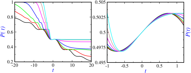
Figure 1: The probability for remaining in the region $x<0$ versus time for the free propagation of the state given by Eq. (20) in the CK framework (left panel). Different values of the friction coefficient are used: $\gamma=0$ (black), $\gamma=0.025$ (red), $\gamma=0.05$ (green), $\gamma=0.1$ (blue), $\gamma=0.2$ (magenta), $\gamma=0.3$ (brown) and $\gamma=0.4$ (cyan). The right panel is a close-up of the left one around the origin.

V Numerical calculations

All numerical calculations in this section are carried out for the initial state given by Eq. (20) working in a system of units where $\hbar=m=1$ with $\sigma_{p}=0.05$, $p_{0b}=0.3$, $p_{0a}=1.4$, $\alpha=1.9$ and $\theta=\pi$. With these values, the amount of backflow is maximal for the non-dissipative dynamics Albarelli-2016 . Thus, from Eq. (19), the probability for finding the particle with a negative momentum is $\approx 7.72\times 10^{-10}$. This means that the initial state in the configuration space is practically constructed by superposition of plane waves with positive momenta.

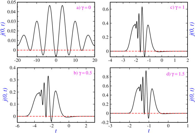
Figure 2: The probability current density at the origin versus time, $j(0,t)$, in the CK framework for four different values of friction coefficient.

Figure 1 (left panel) displays the dissipative quantum backflow in the CK framework. In this figure, we have plotted the probability for remaining in the region $x<0$ versus time for different values of the friction coefficient: $\gamma=0$ (black), $\gamma=0.025$ (red), $\gamma=0.05$ (green), $\gamma=0.1$ (blue), $\gamma=0.2$ (magenta), $\gamma=0.3$ (brown) and $\gamma=0.4$ (cyan). This figure shows that there are some time intervals where the probability for remaining in the negative semi-infinite region increases with time. This is the hallmark of the backflow effect. This is better observed in the right panel of the same figure where a zoom of the time interval around zero is displayed. As observed, the difference between the minima and maxima is slightly reduced by friction and thus the backflow probability.

After Eq. (29), during the backflow intervals where the probability increases, the probability current is negative as clearly observed in Figure 2 where the probability current density at the origin versus time, $j(0,t)$, for four different values of friction coefficient is plotted.

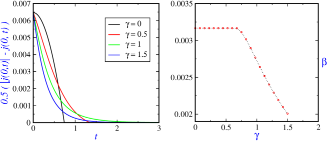
Figure 3: Negative part of the probability current (left panel) and the backflow amount $\beta$ versus $\gamma$ (right panel) in the CK framework.

According to Eq. (29), in order to compute the different backflow probabilities, the time intervals which contain the negative peaks of the probability current should be identified by finding the zeros of this current. Alternatively, another method proposed in Albarelli-2016 is based on the numerical integration of the negative part of the probability current, $0.5(|j(0,t)|-j(0,t))$, over time intervals which contains only a peak. This quantity is plotted in the left panel of Figure 3 for a period of positive times which contains only the highest peak of $0.5(|j(0,t)|-j(0,t))$. The maximum amplitude of such a temporary increase of the probability has been used to quantify this effect Albarelli-2016 ,

$$\beta^{\prime} = \underset{t^{\prime}_{1}<t^{\prime}_{2}}{\sup}[P(t^{\prime}_{2})-P(t^{\prime}_{1})]$$ (72)

where $(t^{\prime}_{1},t^{\prime}_{2})$ represents the different time intervals where the backflow occurs. In the following we use another criterion to quantify the amount of backflow through the numerical integration of the negative part of the probability current over an interval $[t_{1},t_{2}]$ which contains only its highest peak,

$$\beta = \frac{1}{2}\int_{t_{1}}^{t_{2}}dt~{}\{|j(0,t)|-j(0,t)\}.$$ (73)

Due to the dissipation of energy, to arrive at $x=0$ with velocity $\frac{p_{0}}{m}$, the condition $\dot{x}_{t}\rightarrow+\infty$ must be fulfilled at negative times $t\ll-\gamma^{-1}$ for the single Gaussian wavepacket. But, the above condition cannot be fulfilled in practice. Thus, we concentrate our attention to positive times. For comparison, the non-dissipative dynamics should also be considered for positive times. This means that Eq. (73) should be considered for $t_{1}\geq 0$. Using this method, we have computed the backflow amount $\beta$ for different values of friction coefficient and plotted in the right panel of Figure 3. Interesting enough, this amount decreases with friction after a certain plateau at low friction values. If one allows for negative times then the amount of backflow given by Eq. (73) leads to $\beta\approx 0.006323$ for the free non-dissipative dynamics.

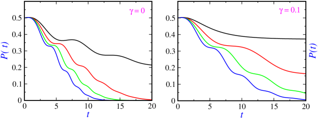
Figure 4: The probability for remaining in the region $x<0$ versus time under the presence of a constant force in the CK framework for the initial state (20) for two values of the friction coefficient: $\gamma=0$ (left panel) and $\gamma=0.1$ (right panel). Different values of the force constant are analyzed: $g=0$ (black curves), $g=0.1$ (red curves), $g=0.2$ (green curves) and $g=0.3$ (blue curves).

Figure 4 highlights the quantum backflow in the CK framework when a constant force is present. In this figure, this effect is studied for non-dissipative and dissipative dynamics separately for different values of the force constant. The corresponding backflow probability for remaining in the region $x<0$ versus time under the presence of a constant force for the initial state (20) and for two values of the friction coefficient, $\gamma=0$ (left panel) and $\gamma=0.1$ (right panel), is plotted. Different values of the force constant are analyzed: $g=0$ (black curve), $g=0.1$ (red curve), $g=0.2$ (green curve) and $g=0.3$ (blue curve). As expected, it is seen in both cases, non-dissipative and dissipative dynamics, that the backflow probability reduces with the force constant.

In subsection IV.1, we have argued that backflow can occur for a single Gaussian wave packet in the CL approach. Occurrence of this backflow has a different nature from the one reported for non-dissipative systems and also dissipative ones in the context of CK, where the backflow originates from quantum interference effects. Here, this backflow seems to be originated directly from the particular dissipative CL dynamics. If we consider free evolution of the state (20) for $\alpha=0$ in the CL framework then, from Eq. (63), one obtains

$$P(t) = \int_{-\infty}^{0}dx\rho(x,t)=\frac{1}{2}\text{erfc}\left[\frac{x_{ta}}{\sqrt{2}w_{t}}\right]$$ (74)

where $x_{ta}$ is the center of the wave packet given by Eq. (12) replacing $p_{0}$ by $p_{0a}$, and $w_{t}$ by Eq. (64). The width of the wavepacket, $w_{t}$, increases with time and this increasing width of the probability distribution works in favour of the appearance of backflow. In the CK case, the increasing of the corresponding width, $\sigma_{t}$, is countered by the motion of the center of the distribution. In figure 5 the probability for remaining in $x<0$ (left panels) and the negative part of the probability density (right panels) have been plotted versus time for two friction coefficients $\gamma=0.1$ (top panels) and $\gamma=0.5$ (bottom panels) and four temperatures, $k_{B}T=1$ (black curves), $k_{B}T=2$ (red curves), $k_{B}T=5$ (green curves) and $k_{B}T=10$ (blue curves). This figure clearly shows there is an important backflow interval starting at $t>0$. The corresponding probability increases with time reaching apparently a constant value.

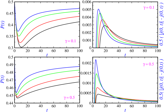
Figure 5: The probability for remaining in $x<0$ versus time in the free propagation of a single Gaussian wave packet, Eq. (20) with $\alpha=0$, within the CL framework for two values of friction coefficients ()$\gamma=0.1$ (top left panel) and $\gamma=0.5$ (bottom left panel)) and four values of temperature, $k_{B}T=1$ (black curves), $k_{B}T=2$ (red curves), $k_{B}T=5$ (green curves) and $k_{B}T=10$ (blue curves). In the right panels, we have plotted the negative part of the probability current density $0.5(|j(0,t)|-j(0,t))$ versus time.

Now we consider the superposition state (20) in the CL framework. The influence of the temperature is studied here within the CL framework. In Figure 6, the probability of finding the particle in the region $x<0$ for free propagation under the CL equation for two values of friction coefficient (0.1 and 0.5) and several temperatures ($k_{B}T=1$ (black curve), $k_{B}T=2$ (red curve), $k_{B}T=5$ (green curve) and $k_{B}T=10$ (blue curve)) is displayed in the top two panels. This figure shows two intervals where the mentioned probability increases i.e., the backflow occurs. A close-up of the first time interval is seen in the bottom two panels. As it is apparent, the amount and duration of this first backflow decreases with temperature for a given friction coefficient. Furthermore, for $\gamma=0.1$, the duration and amount of the first backflow are respectively $\approx 0.657143$ and $\approx 0.002705$ for $k_{B}T=1$ while the corresponding values for $k_{B}T=10$ are $\approx 0.385714$ and $\approx 0.001756$. A similar behavior of the probability is observed at long times with respect to the one Gaussian case.

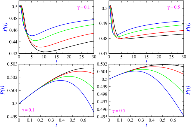
Figure 6: The probability for remaining in $x<0$ versus time in free propagation of the state (20) under the CL equation for different values of friction coefficients: $\gamma=0.1$ (top left panel) and $\gamma=0.5$ (top right panel) for different values of temperature, $k_{B}T=1$ (black curves), $k_{B}T=2$ (red curves), $k_{B}T=5$ (green curves) and $k_{B}T=10$ (blue curves). In the bottom panels we have focused on the first backflow interval.

Finally, in Figure 7 is depicted the probability for remaining in the negative part of $x-$axis for dissipative dynamics with $\gamma=0.1$ at the temperature $k_{B}T=1$ (left top panel) and $k_{B}T=10$ (right top panel) for different values of force constant, $g=0$ (black curve), $g=0.01$ (red curve), $g=0.02$ (green curve) and $g=0.03$ (blue curve). This figure shows again that there is a time interval where the probability for remaining in the negative semi-infinite region increases with time. This is better seen in the bottom panels where a zoom of this interval is plotted. Backflow decreases again with increasing acceleration $g$ for a given temperature. Furthermore, by comparing left and right panels for a given $g$, one observes that the temperature decreases the duration and amount of backflow. For instance, when $g=0.03$ we have $\approx 0.628571$ and $\approx 0.002631$ for $k_{B}T=1$ respectively, and $\approx 0.385714$ and $\approx 0.001734$ for $k_{B}T=10$.

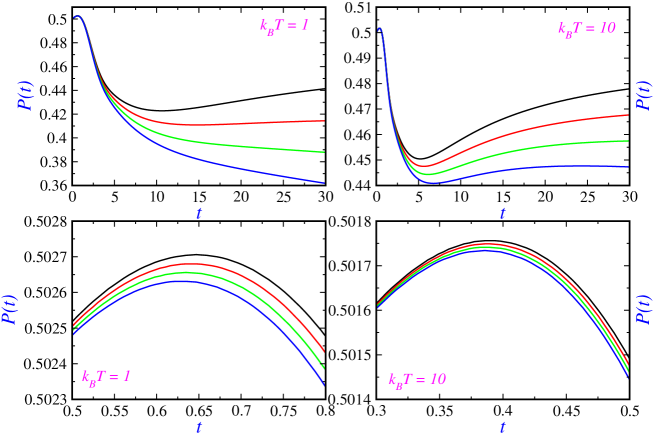
Figure 7: The probability for remaining in $x<0$ versus time in the CL framework for the pure state (20) for $\gamma=0.1$ for different temperatures: $k_{B}T=1$ (top left panel) and $k_{B}T=10$ (top right panel) for different values of acceleration, $g=0$ (black curves), $g=0.01$ (red curves), $g=0.02$ (green curves) and $g=0.03$ (blue curves). In the bottom panels we have focused on the region around the maximum.

VI summary and discussion

In this work, we have studied the backflow effect, that is, negative fluxes for positive-momentum wavepackets for an open quantum system in the CK and CL frameworks. In the CK approach, only friction is taken into account through an effective time-dependent Hamiltonian. In the CL approach, the quantum system under study is coupled to a boson reservoir, i.e., to an infinite number of quantum oscillators at thermal equilibrium. In this approach, both system and its environment is described by a single Hamiltonian. The equation of motion for the reduced density matrix describing the system of interest is obtained by tracing over the degrees of freedom of the environment. In this way, Caldeira and Leggett obtained the master equation (60) in the high-temperature limit. In both CK and CL approaches, the equation of motion for the quantum state is linear. The other approaches that one could choose are the logarithmic non-linear Schrödinger equations MoMi-AO-2018 ; MoMi-EPJP-2019 ; MoMi-Arxiv-2019 and the stochastic Schrödinger equation Percival ; Petruccione . In these approaches, the linearity is not fulfilled and the form of the initial superposed state is not preserved under such dynamics.

As far as we know, this is the first study of dissipative quantum backflow. For a superposition of Gaussian wavepackets with a negligible negative momentum contribution, the backflow also takes place as it has been already reported for the non-dissipative dynamics in free propagation. We have found that the backflow decreases with increasing the parameters of the environment i.e., friction $\gamma$ and temperature $T$ and also observed that it is never suppressed. The constant force $mg\geq 0$ behaves against backflow. Interestingly enough, quantum backflow is also observed for a single Gaussian wave packet within the CL context. Surprisingly, the backflow effect seems to be persistent at long times when considering both one and two Gaussian wave packets. Furthermore, we have studied backflow as an eigenvalue problem in the context of CK framework and concluded that eigenvalues are independent of mass, Planck’s constant, friction and duration of the backflow in free propagation. However, the dynamics under the presence of a constant force is again dependent on those parameters through a dimensionless quantity. Finally, the classical limit has been briefly discussed within a more natural context which is that of the classical Schrödinger equation. Within this scenario, backflow is not suppressed either. Quantum backflow for identical particles (fermions and bosons) in the conservative and non-coservative cases is now in progress.

Acknowledgement

SVM acknowledges support from the University of Qom and SMA support from the Ministerio de Ciencia, Innovación y Universidades (Spain) under the Project FIS2017-83473-C2-1-P. We would like to thank the referees for providing us very important and critical comments.

References

- (1) G. R. Allcock, Ann. Phys 53 (1969) 253; ibid 53 (1969) 286; ibid 53 (1969) 311.
- (2) A. J. Bracken and G. F. Melloy, J. Phys. A Math. Gen. 27 (1994) 2197.
- (3) A. J. Bracken and G. F. Melloy, Ann. Phys. (Leipzig) 7 (1998) 726.
- (4) M. Penz, G. Grübl, S. Kreidl and R. Verch, J. Phys. A 39 (2006) 423.
- (5) J. G. Muga and C. R. Leavens, Phys. Rep. 338 (2000) 353.
- (6) M. V. Berry and S. Popescu, J. Phys. A:Math. Theor. 39 (2006) 6965.
- (7) M. V. Berry, J. Phys. A: Math. Theor. 43 (2010) 415302.
- (8) J. M. Yearsley, J. J. Halliwell, R. Hartshorn and A. Whitby, Phys. Rev. A 86 (2012) 042116.
- (9) J. M. Yearsley and J. J. Halliwell, J. Phys.: Conference Serie 442 (2013) 012055.
- (10) F. Albarelli, T. Guaita and M. G. A. Paris, Int. J. Quantum Inf., 14 (2016) 1650032.
- (11) A. Goussev, Phys. Rev. A, 99 (2019) 043626.
- (12) J. M. Yearsley, Phys. Rev. A 82 (2010) 012116.
- (13) P. Caldirola Nuovo Cimento 18 (1941) 393; E. Kanai Prog. Theor. Phys. 3 (1948) 440.
- (14) A. O. Caldeira and A. J. Leggett, Physica A, 121 (1983) 587.
- (15) A. O. Caldeira, An Introduction to Macroscopic Quantum Phenomena and Quantum Dissipation, Cambridge University Press, 2014.
- (16) S.V. Mousavi and S. Miret-Artés, Ann. Phys. 393 (2018) 76.
- (17) A. S. Sanz, R. Martínez-Casado, H. C. Peñate-Rodriguez, G. Rojas-Lorenzo and S. Miret-Artés, Ann. Phys. 347 (2014) 1.
- (18) C. D. Richardson, P. Schlagheck, J. Martin, N. Vandewalle and T. Bastin, Phys. Rev. A 89 (2014) 032118.
- (19) S.V. Mousavi and S. Miret-Artés, J. Phys. Commun. 2 (2018) 035029.
- (20) S.V. Mousavi and S. Miret-Artés, Eur. Phys. J. Plus, 135 (2020) 83.
- (21) A. Venugopalan, Phys. Rev. A 50 (1994) 2742; A. Venugopalan, D. Kumar and R. Ghosh, Physica A 220 (1995) 563.
- (22) C. R. Leavens: Bohm Trajectory Approach to Timing Electrons, Lect. Notes Phys. 734 (2008) 129–162.
- (23) S.V. Mousavi and S. Miret-Artés, Eur. Phys. J. Plus, 134 (2019) 311.
- (24) S.V. Mousavi and S. Miret-Artés, Eur. Phys. J. Plus, 134 (2019) 431.
- (25) I. Percival, Quantum State Diffusion, Cambridge University Press, Cambridge, 1998.
- (26) H.-P. Bauer and F. Petruccione, The Theory of Open Quantum Systems, Oxford University Press, 2002.