Quasistable charginos in ultraperipheral proton-proton collisions at the LHC

Abstract

We propose a model-independent approach for the search of charged long-lived particles produced in ultraperipheral collisions at the LHC. The main idea is to improve event reconstruction at ATLAS and CMS with the help of their forward detectors. Detection of both scattered protons in forward detectors allows complete recovery of event kinematics. Though this requirement reduces the number of events, it greatly suppresses the background, including the large background from the pile-up.

1 Introduction

The Large Hadron Collider (LHC) can be considered as a photon-photon collider with the photons produced in ultraperipheral collisions (UPC) of charged particles: protons or heavy ions. In such collisions the colliding particles pass near each other exchanging photons; the particles remain intact after the collision. Enormous collision energy achieved at the LHC permits treatment of the particles’ electromagnetic fields as bunches of real photons distributed according to a well-known spectrum. This approximation is known as the equivalent photon approximation (EPA) [1, 2, 3, 4] (see also [5, 6, 7, 8]).

Ultraperipheral collisions are a promising source of New Physics events for the kinds of physics that can appear in photon fusion. They feature clear experimental signature with only the photon fusion result and the two initial particles in the final state. The colliding particles scatter at a very small angle and escape the detector through the beam pipe. They can be registered with forward detectors—ATLAS Forward Proton Detector (AFP) [9] or CMS-TOTEM Precision Proton Spectrometer [10]. These detectors are located at the distance of $\approx 200$ m from the interaction point along the beam pipe, and they can be moved as close as a few millimeters from the beam. Forward detectors can detect a proton with efficiency near 100% if its fractional momentum loss, $\xi\equiv\Delta p/p$, is in the range $0.015<\xi<0.15$ [9, 10]. In the original FP420 proposal [11] forward detectors were placed at 420 m from the interaction point, and the corresponding fractional momentum loss range was at smaller values $0.002<\xi<0.020$. This position at 420 m was not retained in the actual AFP detector, but can be used for estimations of sensitivities. The corresponding energy losses are presented in Table 1. Unfortunately, a heavy ion from lead-lead collisions with the energy of $5.02$ TeV/nucleon pair cannot be detected in forward detectors because the production cross section and EPA spectrum are highly suppressed at $\xi\gtrsim 0.002$.

Table 1: Energy losses required for a particle to be detected in the forward detector placed at different distances from the interaction point (IP).

Distance from the IP, m	200		420
$\xi$ range	$0.015$–	$0.15$	$0.002$–	$0.02$
$6.5$ TeV $p$ energy loss, GeV	$97.5$–	975	13–	130
$0.5$ PeV 208Pb energy loss, TeV	$7.8$–	78	$1.0$–	10

Photon flux in UPC is proportional to $(Z_{1}e)^{2}(Z_{2}e)^{2}$, where $Z_{1}e$ and $Z_{2}e$ are electric charges of the colliding particles. In this respect, collisions of heavy ions, e.g. lead ions with $Z=82$, look much more promising for the search of New Physics. However, in order for the process of photon emission to be coherent, photon virtuality $q^{2}$ where $q$ is the photon 4-momentum has to be smaller than square of the inverse of the charge radius. In the case of proton, calculation based on its electromagnetic form factor results in $\hat{q}=0.20$ GeV [12], where $\hat{q}$ is the maximum momentum of a virtual photon in the proton rest frame. In the laboratory reference frame the maximum photon energy is $\hat{q}\gamma$ where $\gamma$ is the Lorentz $\gamma$-factor of the proton; for a $6.5$ TeV proton $\hat{q}\gamma=1.4$ TeV. For the lead ion, $\hat{q}=30$ MeV [12], so in lead-lead collisions with the energy $5.02~{}\text{TeV}/\text{nucleon pair}$, maximum photon energy is $80$ GeV. Photons with higher energy are produced as well, but their production is suppressed by the nucleus form factor, thus greatly reducing the benefits from higher photon flux in a collision of heavy ions. Nevertheless, the production cross section for a system with invariant mass about 100 GeV is several orders of magnitude larger in lead-lead collisions than in proton-proton collisions [12].

A good example of New Physics that can be searched in UPC is supersymmetry (SUSY) [13, 14, 15, 16, 17]. The supersymmetric partners of the electroweak bosons are six particles: four neutralinos and two charginos. Let $\tilde{\chi}_{1}^{0}$ be the lightest neutralino and $\tilde{\chi}_{1}^{\pm}$ be the lightest chargino. At present, chargino and neutralino with masses below $\sim 1$ TeV are excluded in a large region of SUSY parameters by the LHC results [18, §110.5]. However, most of the searches are much less sensitive to the case when the masses of the lightest chargino and the lightest neutralino are approximately equal. In particular, in the framework of the MSSM, when $m_{\tilde{\chi}_{1}^{\pm}}-m_{\tilde{\chi}_{1}^{0}}\lesssim 2$ GeV, the bound $m_{\tilde{\chi}_{1}^{\phantom{.}}}>92$ GeV comes from the LEP experiments [19]. At this mass scale, the possibility that $m_{\tilde{\chi}_{1}^{\pm}}<m_{\tilde{\chi}_{1}^{0}}$ is excluded, since then the chargino would be stable (assuming $R$-parity conservation), and the charginos remaining after the Big Bang and/or produced in cosmic rays would form hydrogen-like atoms that would be observed in sea water [20, 21, 22, 23] (see also [24]). Thus, in what follows we consider only the case when the lightest chargino is (slightly) heavier than the lightest neutralino. Such compressed chargino-neutralino spectrum is realized in the following two cases: $M_{2}\ll M_{1},\mu$ (wino-like) or $\mu\ll M_{1},M_{2}$ (higgsino-like), where $M_{1}$ is the bino mass parameter, $M_{2}$ is the wino mass parameter, and $\mu$ is the higgsino mass parameter.

In this scenario, chargino might live long enough to fly through the detector and decay outside if they are produced at the LHC. Such particles are called long-lived charged particles (LLCP). In this paper we suggest an approach for the search of LLCP using forward detectors of the ATLAS and CMS collaborations. Although LLCP appear in a variety of models of New Physics, we find SUSY with compressed mass scenario to be the most interesting. Nevertheless, our results can be applied to LLCP of any nature.

There are many searches for long-lived particles in inelastic processes at the LHC [25, 26, 27, 28, 29, 30, 31, 32, 33, 34, 35, 36]. The unobservation of LLCP at the LHC allows the experiments to set model-independent constraints on fiducial LLCP production cross sections. These constraints are then reinterpreted in a particular model to derive bounds on LLCP integrated production cross sections and masses. Therefore, the bounds established in these papers strongly depend on the choice of the supersymmetric model, e.g., on squark masses and/or chargino coupling to $Z$. Further extension of the model with New Physics such as extra Higgs fields or $Z^{\prime}$ bosons will affect these bounds as well. In ultraperipheral collisions, chargino production is mediated by photons which couple to chargino in a model independent way. Consequently, UPC provide us with a way to set model-independent bounds on the masses of charginos (or other long-lived charged particles).

Small cross sections of UPC processes prevent observation of LLCP in the previous searches [25, 26, 27, 28, 29, 30, 31, 32, 33, 34, 35, 36]. See Appendix A for the detailed discussion.

The region of SUSY parameters with $m_{\tilde{\chi}_{1}^{0}}\approx m_{\tilde{\chi}_{1}^{\pm}}\equiv m_{\chi}\sim 100$ GeV can be probed at the LHC in UPC of both protons and heavy ions. Let us consider the cross sections (Section 2), the search strategy (Section 3), the background (Section 4) for chargino production, and the accessible chargino masses and lifetimes (Section 5). In Appendix A we discuss why papers [25, 26, 27, 28, 29, 30, 31, 32, 33, 34, 35, 36] do not exclude the production of charged long-lived particles with masses 100–200 GeV in ultraperipheral collisions.

2 Production cross section

Figure 1: Leading order Feynman diagrams for chargino production in an ultraperipheral collision of two protons.

Consider production of a pair of charginos in an UPC of two identical particles with charge $Ze$. The leading order Feynman diagrams of this process for protons are presented in Fig. 1. Collision is mediated by approximately real photons emitted from the colliding particles. The equivalent photon approximation provides the momentum distribution of these photons [37]:

$$n(\vec{q}_{\perp},\omega)\,\mathrm{d}^{2}q_{\perp}\,\mathrm{d}\omega=\frac{Z^{2}\alpha}{\pi^{2}}\frac{\vec{q}_{\perp}^{\;2}}{\omega\left(\vec{q}_{\perp}^{\;2}+\dfrac{\omega^{2}}{\gamma^{2}}\right)^{2}}\left\lvert F\left(\vec{q}_{\perp}^{\;2}+\frac{\omega^{2}}{\gamma^{2}}\right)\right\rvert^{2}\,\mathrm{d}^{2}q_{\perp}\,\mathrm{d}\omega,$$ (1)

where $\omega$ is the photon energy in the laboratory frame, $\vec{q}_{\perp}$ is the transverse component of the photon momentum, $\gamma$ is the Lorentz factor of the source particle, $F$ is the form factor originating from the vertex involving the particle which emit photons. Let us note that $\vec{q}_{\perp}^{\;2}+(\omega/\gamma)^{2}=-q^{2}$, where $q$ is the photon 4-momentum.

When discussing the form factors it is convenient to use photon 3-momentum in the rest frame of the source particle $\vec{q}=(\vec{q}_{\perp},\omega/\gamma)$. For the proton, the Dirac form factor is [38]

$$F(\vec{q}^{\;2})=G_{D}(\vec{q}^{\;2})\left[1+\frac{(\mu_{p}-1)\tau}{1+\tau}\right],$$ (2)

where

$$G_{D}(\vec{q}^{\;2})\equiv\frac{1}{(1+\vec{q}^{\;2}/\Lambda^{2})^{2}}$$ (3)

is the dipole form factor, $\mu_{p}=2.79$ is the proton magnetic moment, $\tau=\vec{q}^{\;2}/4m_{p}^{2}$, $m_{p}$ is the proton mass, and $\Lambda^{2}=0.71~{}\text{GeV}^{2}$. Since in an UPC $\lvert q^{2}\rvert\lesssim\Lambda_{\text{QCD}}^{2}\ll 4m_{p}^{2}$, the magnetic form factor contribution can be neglected. In this case $F(\vec{q}^{\;2})\approx G_{D}(\vec{q}^{\;2})$, and the equivalent photon spectrum is given by [12]

$$n_{p}(\omega)\,\mathrm{d}\omega=\frac{\alpha}{\pi}\left[(4a+1)\ln\left(1+\frac{1}{a}\right)-\frac{24a^{2}+42a+17}{6(a+1)^{2}}\right]\frac{\mathrm{d}\omega}{\omega},$$ (4)

where $a=(\omega/\Lambda\gamma)^{2}$.

Heavy nucleus form factor is more complicated. The most accurate description of nucleus charge distribution appears to be in the form of Bessel decomposition [39]:

$$\rho(r)=\sum\limits_{n=1}^{N}a_{n}\,j_{0}(n\pi r/R)\,\theta(R-r),$$ (5)

where $j_{0}(x)=\sin x/x$ is the spherical Bessel function of order zero, $\theta(x)$ is the Heaviside step function, $a_{n}$ and $R$ are parameters of the decomposition. The form factor is the Fourier transform of the charge distribution:

$$F(\vec{q}^{\;2})=\frac{\int\rho(r)\mathrm{e}^{i\vec{q}\vec{r}}\mathrm{d}^{3}r}{\int\rho(r)\mathrm{d}^{3}r}=\frac{\sin\lvert\vec{q}\,\rvert R}{\lvert\vec{q}\,\rvert R}\cdot\frac{\sum\limits_{n=1}^{N}\frac{(-1)^{n}a_{n}}{n^{2}\pi^{2}-\vec{q}^{\;2}R^{2}}}{\sum\limits_{n=1}^{N}\frac{(-1)^{n}a_{n}}{n^{2}\pi^{2}}}.$$ (6)

Numerical values of $a_{n}$ and $R$ are provided in Ref. [40]. The corresponding equivalent photon spectrum $n_{\text{Pb}}(\omega)$ is calculated through numerical integration of Eq. (1).

Production of charginos in photon fusion is described by the Breit-Wheeler cross section [41],

$$\sigma(\gamma\gamma\to\tilde{\chi}_{1}^{+}\tilde{\chi}_{1}^{-})=\frac{4\pi\alpha^{2}}{s}\left[\left(1+\frac{4m_{\chi}^{2}}{s}-\frac{8m_{\chi}^{4}}{s^{2}}\right)\ln\frac{1+\sqrt{1-4m_{\chi}^{2}/s}}{1-\sqrt{1-4m_{\chi}^{2}/s}}-\left(1+\frac{4m_{\chi}^{2}}{s}\right)\sqrt{1-\frac{4m_{\chi}^{2}}{s}}\right],$$ (7)

where $\sqrt{s}\equiv\sqrt{4\omega_{1}\omega_{2}}$ is the invariant mass of the pair of charginos, $\omega_{1}$ and $\omega_{2}$ are photons energies. Cross section for charginos production in ultraperipheral collisions is

$$\sigma(NN\to NN\tilde{\chi}_{1}^{+}\tilde{\chi}_{1}^{-})=\int\limits_{0}^{\infty}\int\limits_{0}^{\infty}\sigma(\gamma\gamma\to\tilde{\chi}_{1}^{+}\tilde{\chi}_{1}^{-})\,n_{N}(\omega_{1})\,n_{N}(\omega_{2})\,\mathrm{d}\omega_{1}\,\mathrm{d}\omega_{2},$$ (8)

where $N$ is the colliding particle, $n_{N}(\omega)$ is its equivalent photon spectrum. For $m_{\chi}=100$ GeV,

$$\sigma(pp\to pp\tilde{\chi}_{1}^{+}\tilde{\chi}_{1}^{-})=2.84~{}\text{fb},\ \sigma(\text{Pb}\;\text{Pb}\to\text{Pb}\;\text{Pb}\;\tilde{\chi}_{1}^{+}\tilde{\chi}_{1}^{-})=21.2~{}\text{pb},$$ (9)

where the proton-proton collision energy is 13 TeV, and lead-lead collision energy is $5.02$ TeV/nucleon pair (these parameters correspond to the currently available LHC data). Cross section dependence on chargino mass is presented in Fig. 2. At higher masses chargino pair production in lead-lead collisions is heavily suppressed by the lead ion form factor.

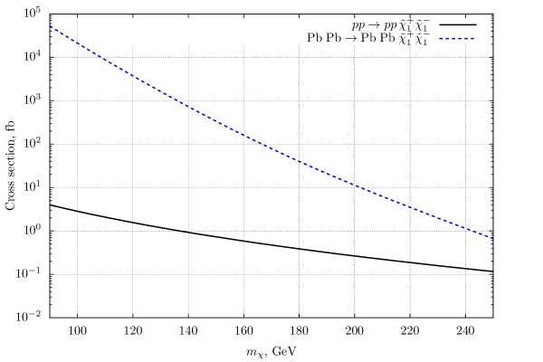
Figure 2: Cross sections for chargino pair production in proton-proton UPC with the collision energy 13 TeV and lead-lead UPC with the collision energy 5.02 TeV/nucleon pair.

In order for both colliding particles to be detected in forward detectors (FD), their momentum loss $\xi=\Delta p/p$ has to be in the interval $\xi_{\text{min}}<\xi<\xi_{\text{max}}$, where $\xi_{\text{min}}=0.015$ and $\xi_{\text{max}}=0.15$ for the ATLAS and CMS experiments [9, 10] (see Table 1). The corresponding cross section is given by formula (8) with cuts on photon energies:

$$\sigma_{\text{FD}}(NN\to NN\tilde{\chi}_{1}^{+}\tilde{\chi}_{1}^{-})=\int\limits_{\xi_{\text{min}}E}^{\xi_{\text{max}}E}\int\limits_{\xi_{\text{min}}E}^{\xi_{\text{max}}E}\sigma(\gamma\gamma\to\tilde{\chi}_{1}^{+}\tilde{\chi}_{1}^{-})\,n_{N}(\omega_{1})\,n_{N}(\omega_{2})\,\mathrm{d}\omega_{1}\,\mathrm{d}\omega_{2},$$ (10)

where $2E$ is the collision energy. For the same parameters as in (9),

$$\sigma_{\text{FD}}(pp\to pp\tilde{\chi}_{1}^{+}\tilde{\chi}_{1}^{-})=0.80~{}\text{fb}.$$ (11)

For lead ions, according to Eq. (9), with the current integrated luminosity $2.5~{}\text{nb}^{-1}$ [46, 47], there will be $0.053$ events. To observe chargino in lead-lead collisions, the integrated luminosity has to be tremendously increased. If the luminosity could be increased by three orders of magnitude, there would be about 50 events. For a lead ion to survive in an UPC, its energy loss should not be much greater than $\approx 100$ GeV [12]. The corresponding value of $\xi$ is $1.9\cdot 10^{-4}$. It makes detection of a lead ion in a forward detector impossible (see Table 1).

Differential cross sections are presented in Fig. 3. Assuming total Run 3 luminosity in proton-proton collisions of 300 fb^-1 at the ATLAS and CMS detectors, the number of produced chargino pairs with both protons detected in forward detectors can be of the order of 250 per detector.

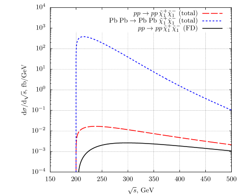
Figure 3: Differential cross sections for chargino pair production in ultraperipheral collisions at the LHC with respect to the chargino pair invariant mass $\sqrt{s}$ (often denoted as $\sqrt{s_{\gamma\gamma}}$ in other papers). $pp\to pp\tilde{\chi}_{1}^{+}\tilde{\chi}_{1}^{-}$ (total) and $\text{Pb}\;\text{Pb}\to\text{Pb}\;\text{Pb}\;\tilde{\chi}_{1}^{+}\tilde{\chi}_{1}^{-}$ (total) are the cross sections integrated over whole phase space. $pp\to pp\tilde{\chi}_{1}^{+}\tilde{\chi}_{1}^{-}$ (FD) is the cross section with the requirement that both protons are detected in forward detectors (FD). The FD cross section for lead-lead collisions is many orders of magnitude less, and its threshold is at $\sqrt{s}\approx 15$ TeV, because both lead ions have to lose at least $7.8$ TeV of their energy to hit forward detectors (see Table 1). Here chargino mass is assumed to be 100 GeV, $pp$ collision energy is 13 TeV, Pb Pb collision energy is $5.02~{}\text{TeV}/\text{nucleon pair}$.

In the LHC experiments, some regions of the phase space of produced particles are cut off. Common requirements for a particle to be detected in the muon system are $p_{T}>\hat{p}_{T}$ and $\lvert\eta\rvert<\hat{\eta}$, where $p_{T}$ is the particle transverse momentum, $\eta$ is its pseudorapidity, and $\hat{p}_{T}$ and $\hat{\eta}$ are experimental cuts on these values. The corresponding (fiducial) cross section for the $pp\to pp\,\tilde{\chi}_{1}^{+}\tilde{\chi}_{1}^{-}$ reaction is (see [12] for the derivation of this formula with $m_{\chi}=0$)

$$\sigma_{\text{fid.}}(pp\to pp\,\tilde{\chi}_{1}^{+}\tilde{\chi}_{1}^{-})=\\ =\int\limits_{(2\xi_{\text{min}}E)^{2}}^{(2\xi_{\text{max}}E)^{2}}\mathrm{d}s\int\limits_{\max\left(\hat{p}_{T},\frac{\sqrt{s/4-m_{\chi}^{2}}}{\cosh\hat{\eta}}\right)}^{\sqrt{s/4-m_{\chi}^{2}}}\mathrm{d}p_{T}\,\frac{\mathrm{d}\sigma(\gamma\gamma\to\tilde{\chi}_{1}^{+}\tilde{\chi}_{1}^{-})}{\mathrm{d}p_{T}}\int\limits_{1/\hat{x}}^{\hat{x}}\frac{\mathrm{d}x}{8x}\,n\left(\sqrt{\frac{sx}{4}}\right)\,n\left(\sqrt{\frac{s}{4x}}\right),$$ (12)

where $x=\omega_{1}/\omega_{2}$, and

$$\hat{x} =\left(\hat{X}+\sqrt{\hat{X}^{2}+1}\right)^{2},$$ (13)

$$\hat{X} =\frac{\sqrt{s}\,p_{T}}{2(p_{T}^{2}+m_{\chi}^{2})}\left(\sinh\hat{\eta}-\sqrt{\cosh^{2}\hat{\eta}+\frac{m_{\chi}^{2}}{p_{T}^{2}}}\cdot\sqrt{1-\frac{4(p_{T}^{2}+m_{\chi}^{2})}{s}}\right).$$

The differential with respect to $p_{T}$ cross section is

$$\frac{\mathrm{d}\sigma(\gamma\gamma\to\tilde{\chi}_{1}^{+}\tilde{\chi}_{1}^{-})}{\mathrm{d}p_{T}}=\frac{8\pi\alpha^{2}p_{T}}{s(p_{T}^{2}+m_{\chi}^{2})}\cdot\frac{1-\dfrac{2(p_{T}^{4}+m_{\chi}^{4})}{s(p_{T}^{2}+m_{\chi}^{2})}}{\sqrt{1-\dfrac{4(p_{T}^{2}+m_{\chi}^{2})}{s}}}.$$ (14)

For

$$m_{\chi} =100~{}\text{GeV}, E =6.5~{}\text{TeV},$$ (15)

$$\xi_{\text{min}}E =97.5~{}\text{GeV}, \xi_{\text{max}}E =975~{}\text{GeV},$$

$$\hat{p}_{T} =20~{}\text{GeV}, \hat{\eta} =2.5,$$

we get

$$\sigma_{\text{fid.}}(pp\to pp\,\tilde{\chi}_{1}^{+}\tilde{\chi}_{1}^{-})=0.72~{}\text{fb}.$$ (16)

The differential fiducial cross section is presented in Fig. 4. Integrated fiducial cross section for a range of chargino masses is presented in Fig. 5.

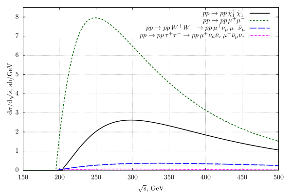
Figure 4: Differential fiducial cross sections for the reaction $pp\to pp\,\tilde{\chi}_{1}^{+}\tilde{\chi}_{1}^{-}$ and its backgrounds with respect to the invariant mass of the produced system.

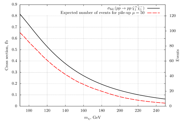
Figure 5: Upper curve: fiducial cross section for the $pp\to pp\;\tilde{\chi}_{1}^{+}\tilde{\chi}_{1}^{-}$ reaction with respect to chargino mass. Lower curve: expected number of events in the LHC data collected in Run 2 (for the integrated luminosity 150 fb^-1) assuming constant pile-up $\mu=50$ and after applying the cut (25).

3 Search strategy

Assuming $R$-parity conservation, with the lightest chargino and the lightest neutralino masses being nearly equal, it is possible that $\tilde{\chi}_{1}^{\pm}$ lives long enough to escape the detector and decay outside. The experimental signature and, consequently, the background of the chargino production process greatly depend on the stability of chargino. There are three possible scenarios: 1. Chargino decays in the beam pipe of the detector. This scenario will not be studied in this paper. For model-dependent bounds see, e.g., [48, 49]. 2. Chargino decays in the body of the detector producing a disappearing track in the detector. This scenario is studied in Ref. [50, 51] in the framework of minimal anomaly mediated symmetry breaking model (mAMSB), and charginos with the mass 100 GeV and lifetime above 0.02 ns and below few 100 ns are excluded. These searches require high energetic jet from initial state radiation in chargino production events, so their bounds are not applicable for chargino production in ultraperipheral collisions. This scenario will not be further studied in this paper. 3. Chargino decays outside the detector producing a track in the detector.

Let us consider the case when chargino lives long enough to escape the detector (case 3). Then a track from a charged particle will be observed in the detector. Since in the Standard Model only a muon can go through the full detector (including the outer muon spectrometers), the question is whether a chargino can be distinguished from a muon. The common approach for the search for long-lived charged heavy particles is to measure their energy loss ($\mathrm{d}E/\mathrm{d}x)$ and time of flight through the detector (TOF) [25, 26, 27, 28, 29, 30, 31, 32, 33, 34, 35, 36]. An advantage of UPC is that the event kinematics can be fully reconstructed by measuring the proton energies in forward detectors. In what follows we will study the possibilities provided by this feature of UPC. The method proposed can be complemented by the conventional $\mathrm{d}E/\mathrm{d}x$ and TOF measurements.

For the reaction $pp\to pp\tilde{\chi}_{1}^{+}\tilde{\chi}_{1}^{-}$, momenta of all four particles in the final state can be measured: momenta of chargino candidates $\vec{p}_{1}$, $\vec{p}_{2}$ can be reconstructed from their tracks in the detector, and final state protons can be detected by the forward detectors thus providing their energy losses $\xi_{1}$, $\xi_{2}$ (protons transverse momenta can be neglected). The observable suitable for the discovery of chargino in UPC is the mass of the charged particle

$$m=\sqrt{\frac{1}{4}\left(E(\xi_{1}+\xi_{2})+\frac{\vec{p}_{1}^{\;2}-\vec{p}_{2}^{\;2}}{E(\xi_{1}+\xi_{2})}\right)^{2}-\vec{p}_{1}^{\;2}}=\frac{\sqrt{\left(E^{2}(\xi_{1}+\xi_{2})^{2}-(\vec{p}_{1}^{\;2}+\vec{p}_{2}^{\;2})\right)^{2}-4\vec{p}_{1}^{\;2}\vec{p}_{2}^{\;2}}}{2E(\xi_{1}+\xi_{2})},$$ (17)

$$m=\sqrt{\frac{(2\xi_{1}\xi_{2}E^{2}+\vec{p}_{1}\vec{p}_{2})^{2}-\vec{p}_{1}^{\;2}\vec{p}_{2}^{\;2}}{4\xi_{1}\xi_{2}E^{2}+(\vec{p}_{1}+\vec{p}_{2})^{2}}}.$$ (18)

Eqs. (17) and (18) are equivalent due to momentum conservation law, however experimental uncertainties give different contributions to these formulas, so both of them are useful when dealing with experimental data. In what follows we will use (18), which is less affected by finite detector resolution. Calculating the mass according to (18) for every event with exactly two charged tracks and two protons detected in forward detectors, and plotting the number of such events with respect to $m$, one should get $\delta(m-m_{\chi})$ smeared with the detector resolution.

4 Background

4.1 Muons

A long-lived chargino produces a signal in the detector very similar to that of a muon. Therefore, the sources of the background are the reactions producing a pair of muons. We consider the following processes:

1. $pp\to pp\,\mu^{+}\mu^{-}$.

2. $pp\to pp\,W^{+}W^{-}\to pp\,\mu^{+}\nu_{\mu}\,\mu^{-}\bar{\nu}_{\mu}$.

3. $pp\to pp\,\tau^{+}\tau^{-}\to pp\,\mu^{+}\nu_{\mu}\bar{\nu}_{\tau}\,\mu^{-}\bar{\nu}_{\mu}\nu_{\tau}$.

Eq. (12) with $m_{\chi}$ replaced with $m_{\mu}$ also works for the $pp\to pp\,\mu^{+}\mu^{-}$ reaction. Fiducial cross sections for the $pp\to pp\,W^{+}W^{-}\to pp\,\mu^{+}\nu_{\mu}\,\mu^{-}\bar{\nu}_{\mu}$ and $pp\to pp\,\tau^{+}\tau^{-}\to pp\,\mu^{+}\nu_{\mu}\bar{\nu}_{\tau}\,\mu^{-}\bar{\nu}_{\mu}\nu_{\tau}$ reactions were calculated with the help of the Monte Carlo method. Parameters of the calculation are defined in Eq. (15). Cross section for the $\gamma\gamma\to W^{+}W^{-}$ process is [52]

$$\sigma(\gamma\gamma\to W^{+}W^{-})=\\ =\frac{8\pi\alpha^{2}}{m_{W}^{2}}\left[\left(1+\frac{3m_{W}^{2}}{4s}+\frac{12m_{W}^{4}}{s^{2}}\right)\sqrt{1-\frac{4m_{W}^{2}}{s}}-\frac{3m_{W}^{4}}{4s^{2}}\left(1-\frac{2m_{W}^{2}}{s}\right)\ln\frac{1+\sqrt{1-4m_{W}^{2}/s}}{1-\sqrt{1-4m_{W}^{2}/s}}\right].$$ (19)

The results are presented in Fig. 4 and Table 2.

Table 2: Fiducial cross sections for the $pp\to pp\,\tilde{\chi}_{1}^{+}\tilde{\chi}_{1}^{-}$ reaction and its backgrounds.

Reaction	Cross section, fb
$pp\to pp\,\tilde{\chi}_{1}^{+}\tilde{\chi}_{1}^{-}\quad(m_{\chi}=100~{}\text{GeV})$	$0.72$
$pp\to pp\,\mu^{+}\mu^{-}$	$1.60$
$pp\to pp\,W^{+}W^{-}\to pp\,\mu^{+}\nu_{\mu}\,\mu^{-}\bar{\nu}_{\mu}$	$0.15$
$pp\to pp\,\tau^{+}\tau^{-}\to pp\,\mu^{+}\nu_{\mu}\bar{\nu}_{\tau}\,\mu^{-}\bar{\nu}_{\mu}\nu_{\tau}$	$0.02$

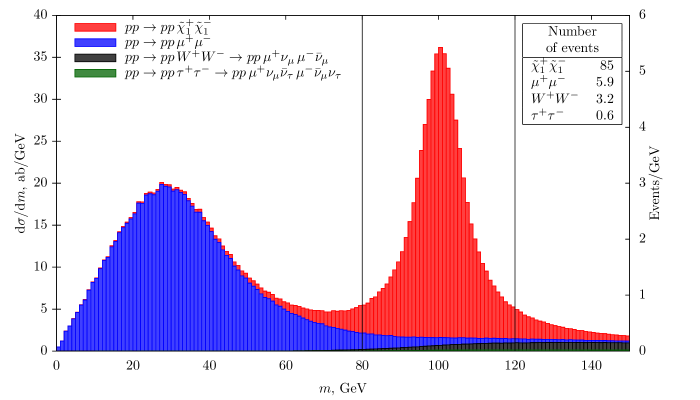
Figure 6: Monte Carlo simulation of the chargino candidate mass distribution. Here and in subsequent plots parameters of the calculation are defined in Eq. (15), the integrated luminosity is assumed to be 150 fb^-1, bin width is 1 GeV and the values in the inset are the total number of the events in between the vertical lines.

Chargino candidate mass distributions according to Eq. (18) for the signal and background processes were calculated by means of the Monte Carlo method. Finite central detector resolution was taken into account according to [53, Section 4.5]. Finite forward detector resolution was taken into account by replacing in (18) $\xi_{i}E$ with a random number normally distributed around $\xi_{i}E$ with the standard variation linearly interpolated with pivot points 5 GeV for $\xi_{i}=0.04$ and 10 GeV for $\xi_{i}=0.14$, in accordance with [9, Section 3.3.2]. The results are presented in Fig. 6. In the case of muons, in half of the events $m^{2}$ is negative, and such events were discarded. When changing from the distribution with respect to $m^{2}$ to the distribution with respect to $m$, an extra factor of $m$ from the Jacobian results in the distribution being 0 at $m=0$ (see Appendix B). This effect is mostly irrelevant for charginos which peak is far from $m=0$. The peak of charginos is well separated from the peak of muons. The background from $W^{+}W^{-}$ and $\tau^{+}\tau^{-}$ production and decay is negligible. Note that the background with neutrinos in the final state can be further heavily suppressed by the requirement that $p_{T1}+p_{T2}=0$ where $p_{Ti}$ are transverse momenta of the detected particles.

4.2 Pile-up

Another important source of background is pile-up. During Run 2 of the LHC, the pile-up was increasing from 25 to 38 collisions per bunch crossing on average, reaching over 70 collisions in some events [46, 47]. In what follows we consider a bunch crossing with $\mu=50$ collisions. It is possible that in one of the collisions, a pair of muons is produced with the energies high enough to pass the cuts on transverse momentum, but not high enough for the proton(s) to be detected in the forward detector(s). At the same time in one or more of the other 49 collisions, another event might happen which results in the proton hitting the forward detector yet the produced particles (e.g., pions) do not pass the trigger thresholds or escape the detector through the beam pipe. In this case the muons from the original event and the protons from the pile-up will mimic the production of a chargino pair with relevant chargino masses.

The most probable event resulting in a proton hitting the forward detector is proton diffractive dissociation which produces a few low-energy pions which escape detection [54]. Proton diffractive dissociation is described by the triple-Regge diagrams [55]. In Appendix B of Ref. [56], the probability for a proton after dissociation to hit the forward detector was estimated to be $P_{\text{SD}}(1)\approx 0.01$ for $0.02<\xi<0.15$. The probability to observe one or more of such protons in a single bunch crossing is

$$P_{\text{SD}}(\mu)=1-(1-P_{\text{SD}}(1))^{\mu}.$$ (20)

$P_{\text{SD}}(50)\approx 0.39$, or, in other words, about 40% of bunch crossings with 50 collisions at once produce at least one proton hitting one of the forward detectors. Following Ref. [57], we shall use the low-$\xi$ approximation for the differential cross section of proton dissociation in the form

$$M_{X}^{2}\frac{\mathrm{d}\sigma}{\mathrm{d}M_{X}^{2}}\propto 1+\frac{2~{}\text{GeV}}{M_{X}},$$ (21)

where $M_{X}$ is the invariant mass of the system produced. Since $\xi=M_{X}^{2}/4E^{2}$, this expression can be rewritten as

$$\xi\frac{\mathrm{d}\sigma}{\mathrm{d}\xi}\propto 1+\frac{\varkappa}{\sqrt{\xi}},$$ (22)

where $\varkappa=2~{}\text{GeV}/\,13~{}\text{TeV}=1.5\cdot 10^{-4}$. The corresponding spectrum of dissociated protons hitting the forward detector per bunch crossing is

$$f_{p}(\mu,\xi)=P_{\text{SD}}(\mu)\cdot\frac{\,\mathrm{d}\sigma/\mathrm{d}\xi}{\int\limits_{\xi_{\text{min}}}^{\xi_{\text{max}}}\frac{\mathrm{d}\sigma}{\mathrm{d}\xi}\,\mathrm{d}\xi}=\frac{P_{\text{SD}}(\mu)\cdot\dfrac{1}{\xi}\left(1+\dfrac{\varkappa}{\sqrt{\xi}}\right)}{\ln\dfrac{\xi_{\text{max}}}{\xi_{\text{min}}}-\dfrac{\varkappa}{2}\left(\dfrac{1}{\sqrt{\xi_{\text{max}}}}-\dfrac{1}{\sqrt{\xi_{\text{min}}}}\right)}.$$ (23)

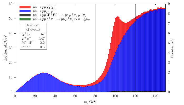
Figure 7: Monte Carlo simulation of the chargino candidate mass distribution with the pile-up background ($\mu=50$).

The results of Monte Carlo simulation with pile-up value $\mu=50$ are presented in Fig. 7. In this case the background is much larger than the signal. The reason is that the equivalent photon spectrum increases at low photon energies, so production of a pair of muons in an UPC is much more probable than production of a pair of charginos with the mass 100 GeV. With no pile-up events, the background from muons was suppressed by the lower bound of the forward detector acceptance region $\xi_{\text{min}}$: if the invariant mass of the muon pair was less than $2\xi_{\text{min}}E=195$ GeV, both protons could not hit the forward detectors simultaneously. With the pile-up enabled, one or two of the protons can come from the pile-up. In Fig. 7 events with multiple hits in forward detectors were discarded.

The advantage of ultraperipheral collisions in the case of pair production of quasistable charginos is that all particles in the final state can be detected and their momenta can be measured. This information can be used to greatly suppress the pile-up background. The total 3-momentum of the colliding system is zero. Its longitudinal component after the collision,

$$p_{\parallel,1}+p_{\parallel,2}+(1-\xi_{1})E-(1-\xi_{2})E=0,$$ (24)

where $p_{\parallel,1}$, $p_{\parallel,2}$, $(1-\xi_{1})E$, and $-(1-\xi_{2})E$ are longitudinal components of momenta of the charginos and the protons. In the case of the pile-up, one or both of the protons are produced in a different event, and this equation is violated. Hence, the background is suppressed by the cut

$$\lvert p_{\parallel,1}+p_{\parallel,2}-(\xi_{1}-\xi_{2})E\rvert<\hat{p}_{\parallel}.$$ (25)

This cut also suppresses the background from $W^{+}W^{-}$ and $\tau^{+}\tau^{-}$ production since neutrinos carry away longitudinal momentum.

Chargino mass distribution for the same parameters as in Fig. 6 with the pile-up value $\mu=50$ was calculated with the help of the Monte Carlo method. The value of $\hat{p}_{\parallel}$ was chosen to be 20 GeV. The result is presented in Fig. 8. In the case of multiple hits in forward detectors, the pair of protons which satisfies Eq. (25) was selected (events with more than one such pair were discarded). This restores the signal events that were discarded due to pile-up in Fig. 7 almost to the number that was available with no pile-up in Fig. 6. The background from $W^{+}W^{-}$ and $\tau^{+}\tau^{-}$ production is less than $0.15$ ab/GeV.

The total number of events expected to be observed in Run 2 data depending on chargino mass is shown in Fig. 5.

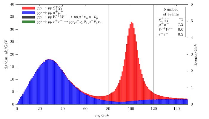
Figure 8: Monte Carlo simulation of the chargino candidate mass distribution with the pile-up background and the cut on the longitudinal momentum of the final state system (25).

5 Accessible masses and lifetimes

So far we were considering charginos living long enough to escape the detector. However, chargino can decay in the detector reducing the number of events that can be reconstructed with our method. In this section we will estimate the range of chargino lifetimes that would allow for the observation of charginos with the LHC data collected during Run 2 assuming that forward detectors operated at 100% efficiency.

For that purpose we have implemented the possibility for chargino decay in our Monte Carlo simulations. Both charginos have to escape the detector for the event to be selected. Chargino candidate mass distributions were calculated for a set of chargino masses $m_{\chi}$ and lifetimes $\tau_{\chi}$ for the pile-up $\mu=50$. For each distribution the mass range $m_{\chi}-10~{}\text{GeV}<m<m_{\chi}+10~{}\text{GeV}$ was selected and the corresponding number of signal events $n_{\chi}$ from the $pp\to pp\tilde{\chi}_{1}^{+}\tilde{\chi}_{1}^{-}$ reaction and the total number of events $n$ including the background processes were calculated. Significance was estimated as $S=n_{\chi}/\sqrt{n}$. Fig. 9 shows isolines of $S$ corresponding to $S=3$ and $S=5$. The largest chargino mass that can be observed at the level of 3 standard deviations is 190 GeV. Chargino candidate mass distribution for stable chargino with the mass 190 GeV is presented in Fig. 10. In the region of masses from 180 to 200 GeV the signal is 11 events, the background is $3.7$ events.

Our results do not take into account the reduction of the number of events due to trigger and reconstruction efficiency. In Ref. [58], the reconstruction efficiency for the $pp\to pp\mu^{+}\mu^{-}$ reaction was estimated at the level of $\varepsilon=0.4$. To demonstrate the effect of efficiency, we have reduced the number of events correspondingly and presented the isolines of $S$ for this value in Fig. 9 as well.

Decaying charginos will leave disappearing tracks in the detector. If the chargino lifetime is too small for chargino to be observed with the method proposed, the latter can be complemented by the search for disappearing tracks. Existing searches for disappearing tracks [50, 51] require a jet in the final state which will not be present in the case of ultraperipheral collisions.

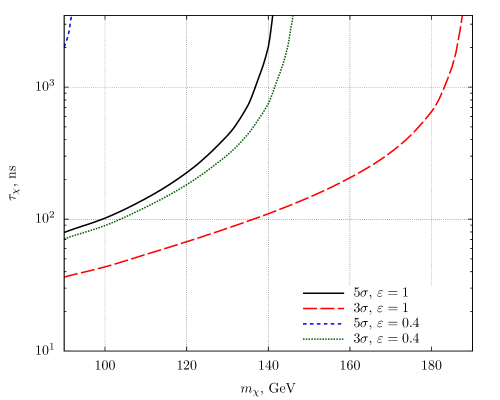
Figure 9: Lower bounds on the values $(m_{\chi},\tau_{\chi})$ that could be observed with the LHC Run 2 data. $3\sigma$ and $5\sigma$ are the signal significances. $\varepsilon$ is the trigger and reconstruction efficiencies. Here ATLAS detector geometry and resolution were used.

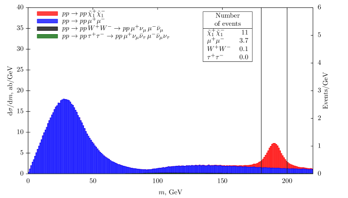
Figure 10: Same as Fig. 8, but with chargino mass set to 190 GeV.

6 Conclusions

Ultraperipheral collisions of protons allow production of heavy charged particles in very clean events. Its cross section is unambiguously determined by the electric charge and the mass of the particles produced and it does not depend on the particular model of New Physics. Measurement of momenta of heavy long-lived charged particles in the main detector complemented by the measurement of protons momenta in forward detectors allows complete reconstruction of event kinematics. With the LHC Run 2 data the range of particle masses available for observation at the level of 3 standard deviations reaches 190 GeV (see Figs. 5 and 10). Accessible masses and lifetimes are shown in Fig. 9. Particles with the lifetime greater than 100 ns can be observed with the method proposed. In view of these results, the operation of the ATLAS and CMS forward detectors during Run 3 will allow for the discovery of new heavy quasistable charged particles provided they exist.

Ultraperipheral lead-lead collisions provide orders of magnitudes greater production cross section than the proton-proton collisions (see Fig. 2). However, complete reconstruction of kinematics with the help of forward detectors is impossible in the case of lead-lead collisions because the required energy loss is too large. New particles can still be searched for with conventional methods based on the ionization energy loss and time-of-flight measurements. These measurements will benefit from the very clean final state of ultraperipheral collisions even in the case of collisions of lead ions. In order to look for long-lived charged particles in lead-lead collisions, the integrated luminosity should be increased by 2–3 orders of magnitude (see the text after Eq. (11)). This call for significantly larger future heavy ion runs and/or runs with lighter ions is discussed in detail in Ref. [59].

7 Acknowledgments

We are grateful to K. G. Boreskov, A. D. Stepennov and I. I. Tsukerman for useful discussions, and to V. A. Khoze for bringing to our attention the large pile-up background. We thank the unknown referee for the comments that helped to substantially improve the paper. The authors are supported by the Russian Science Foundation grant No 19-12-00123.

Appendix A On preceding searches for heavy charged long-lived particles

If heavy long-lived charged particles (LLCP) exist and have masses 100–200 GeV, they would have already been produced in ultraperipheral collisions at the LHC. They could be observed in searches which do not require large missing energy or jets in the final state. Most of Refs. [25, 26, 27, 28, 29, 30, 31, 32, 33, 34, 35, 36] look for events with two well-separated muon-like tracks with large transverse momentum not accompanied by hadronic jets. We shall discuss why these studies do not exclude LLCP with the masses 100–200 GeV produced in $pp$ UPC.

Ref. [25] is devoted to the search for heavy stable charged particles in $pp$ collisions at the collision energy 7 TeV. Production cross section in UPC (8) at this energy is $1.19$ fb for chargino mass 100 GeV, and it decreases when the mass increases. With the integrated luminosity studied in this paper ($3.1~{}\text{pb}^{-1}$), no events are expected.

In Ref. [26], the collision energy is 7 TeV as well, but the integrated luminosity is about one order of magnitude larger ($37~{}\text{pb}^{-1}$). However, the luminosity is still too low for even a single $\tilde{\chi}_{1}^{+}\tilde{\chi}_{1}^{-}$ pair to be produced.

In Ref. [27], $5~{}\text{fb}^{-1}$ of integrated luminosity in 7 TeV $pp$ collisions are analyzed. According to (8), 6 events of chargino pair production are expected in this data. For an event to be selected, transverse momentum of each LLCP was required to be larger than $\hat{p}_{T}=40$ GeV and its pseudorapidity to be less than $\hat{\eta}=2.1$. With the help of Eq. (12), setting $\xi_{\text{min}}=0$, $\xi_{\text{max}}=1$ (so each proton can miss the forward detector), we get the corresponding fiducial cross section of $0.65$ fb. 3 events passing these experimental cuts are expected, and even no observation is compatible with this expectation. Additional cuts implemented in Ref. [27] will further diminish the number of events.

In Ref. [28], $5.0~{}\text{fb}^{-1}$ of data at the collision energy 7 TeV and $18.8~{}\text{fb}^{-1}$ of data at the collision energy 8 TeV are analyzed. The selection criteria for LLCP are $p_{T}>70$ GeV, $\lvert\eta\rvert<2.1$. The strongest bound comes from the analysis taking both the $\mathrm{d}E/\mathrm{d}x$ and time-of-flight (TOF) measurements into account. As is shown in Table 3 of that paper, the expected number of background events for $m_{\chi}>100$ GeV is $1.0\pm 0.2$ for the collision energy 7 TeV and $5.6\pm 1.1$ for the collision energy 8 TeV. The number of observed events are 3 and 7 correspondingly. Cross section for pair production of LLCP with the mass 100 GeV in UPC passing the selection criteria is $0.47$ fb ($0.57$ fb) for 7 (8) TeV which corresponds to $2.3$ ($10.7$) events. To compare these numbers with the number of observed events, the former should be multiplied by the detector efficiency. From Table 3 and Figure 8 of the paper we estimate the detector efficiency to be less than 20% for $m_{\chi}=100$ GeV. The resulting number of events is compatible with the background fluctuation.

In Ref. [29], $19.1~{}\text{fb}^{-1}$ of integrated luminosity in 8 TeV $pp$ collisions are analyzed. The relevant signal region is SR-CH-2C which considers chargino pair production with two charged tracks observed in the detector. The cuts on the phase space are $p_{T}>70$ GeV, $\lvert\eta\rvert<2.5$. Chargino mass is varied in the interval 100–800 GeV, but the results are presented only for $m_{\chi}>450$ GeV. As is shown in Table 6, for $m_{\chi}=500$ GeV, the detector efficiency is $0.061\pm 0.003$. The cross section for production of a pair of LLCPs with the mass 100 GeV in UPC is $0.66$ fb, so the number of expected events in this amount of data is $12.6$. Assuming that the detector efficiency does not exceed 10% for $m_{\chi}=100$ GeV, we obtain that only about 1 event is expected. No events observed is consistent with this expectation.

Ref. [30] sets bounds on pMSSM and AMSB models using the results of Ref. [28].

Ref. [31] considers production of metastable charged particles which decay inside the detector. Only the events with the missing energy $E_{T}^{\text{miss}}>80$ GeV were selected. There is no missing energy in pair production of LLCP in UPC, so such events would not be seen in this analysis.

In Ref. [32], the LHCb collaboration searches for the LLCP with the ring imagining Cherenkov detectors. 1 fb^-1 of data collected at $pp$ collisions with the energy 7 TeV and 2 fb^-1 of data collected at $pp$ collisions with the energy 8 TeV are used in this analysis. For an event to be selected, both LLCP candidates have to have $p_{T}>50$ GeV and hit the detector located at $1.8<\eta<4.9$. Cross section for pair production of LLCP with the mass $m_{\chi}=100$ GeV in UPC of protons with the energy 8 TeV satisfying the selection criteria is definitely less than $0.45$ fb. The predicted number of events is less than 1. The background from the $Z/\gamma^{*}\to\mu^{+}\mu^{-}$ reaction is much larger than 1. Therefore, production of LLCP in UPC cannot be observed in this experiment with the current amount of data.

In Ref. [33], the ATLAS collaboration searches for long-lived $R$-hadrons. As in Ref. [31], large missing energy ($E_{T}^{\text{miss}}>70$ GeV) is required, so this search is not sensitive to ultraperipheral collisions.

In Ref. [34], $2.5~{}\text{fb}^{-1}$ of $pp$ collisions with the energy 13 TeV are analyzed. Cross section for pair production of LLCP with the mass 100 GeV in UPC at this energy is $2.84$ fb (9), so $7.1$ events are expected in the data. For the analysis, the events with $p_{T}>55$ GeV and $\lvert\eta\rvert<2.1$ were selected. The UPC cross section diminishes to $1.21$ fb which corresponds to $3.0$ events. As is shown in Table 1 of that paper, 4 events were observed with the predicted number of background events $5.4\pm 1.1$. Even not taking into account the detector efficiency (30–40%, see Tables 5, 6), LLCP pair production in ultraperipheral collisions cannot be excluded.

In Ref. [35], as in Ref. [33], long-lived $R$-hadrons are searched for. Large missing energy (over 170 GeV) is required for an event to be selected. This search is not sensitive to ultraperipheral collisions.

In Ref. [36], $36.1~{}\text{fb}^{-1}$ of integrated luminosity in proton-proton collisions with the energy of 13 TeV is studied. Several signal regions are considered in the paper. The most sensitive region for LLCP pair production in UPC is SR-2Cand-FullDet which requires two tracks from charged particles with $p_{T}>70$ GeV and $\lvert\eta\rvert<2.0$. The corresponding fiducial cross section for $m_{\chi}=100$ GeV is $0.97$ fb. However, the region $m_{\chi}<200$ GeV was used as a control region in the paper. The fiducial cross section in UPC for $m_{\chi}=200$ GeV is $0.14$ fb which corresponds to $5.1$ events. The total cross section (not taking the experimental cuts into account) is $0.27$ fb. According to Table 8, the product of detector acceptance and efficiency is equal to $0.083\pm 0.003$ for the process considered in the paper. Assuming that the detector acceptance for LLCP pair production in UPC is approximately the same as in the process considered in the paper, the detector efficiency is $\sim 0.083/(0.14/0.27)\approx 16$%, so only $0.8$ events of LLCP pair production in UPC are expected in this study.

We see that the cross sections of LLCP pair production in UPC convoluted with actual detection efficiencies and luminosities are too small for these particles to be detected in Refs. [25, 26, 27, 28, 29, 30, 31, 32, 33, 34, 35, 36].

Due to pile-up, an ultraperipheral collision in which a LLCP pair is produced may be accompanied by another collision with large missing energy. However, taking into account that the number of charginos produced in UPC in the papers considered above are of the order of 10, while cross section of the events with large missing energy is many orders of magnitudes less than the total $pp$ cross section ($\sim 100$ mb), the probability of such a coincidence is negligible.

Appendix B The shape of the reconstructed mass distribution

The reader may still be puzzled why the maximum of the reconstructed mass distribution is at the value $\sim 30~{}\text{GeV}$ for muon background rather than at the muon mass. This happens because we plot the reconstructed mass distributions while the width of the squared mass distribution is much larger than its mean value, i.e. the squared muon mass. The value of $\sim 30~{}\text{GeV}$ is defined by detector resolution and the energy spectrum of the muon background.

To illustrate this let us consider the following simple example. For the monochromatic muon beam with energy $E_{\rm beam}$ two independent systems measure the muons energy (analogous to forward detectors providing us with the protons energy losses and therefore with particle energies) and momentum (analogous to the central detector). Due to final resolutions of these systems, $\varepsilon_{\rm E}$ and $\varepsilon_{\rm p}$, reconstructed energy $E_{\rm rec}$ and momentum $p_{\rm rec}$ are not $\delta$-functions but distributed around central values $E_{\rm beam}$ and $p_{\rm beam}=\sqrt{E_{\rm beam}^{2}-m^{2}}$, where $m\approx 0.105~{}\text{GeV}$. For $\varepsilon_{\rm E}=\varepsilon_{\rm p}=5\%$ the distributions for $E_{\rm rec}$ and $p_{\rm rec}$ are shown in Fig. 11(a), 11(b).

With measured energy and momentum for each muon, the mass can be reconstructed as $m_{\rm rec}^{2}=E_{\rm rec}^{2}-p_{\rm rec}^{2}$. The corresponding distribution is shown in Fig. 11(c). It has a peak at the squared muon mass (indistinguishable from 0) as expected.

To plot the same data with respect to $m_{\rm rec}=\sqrt{m_{\rm rec}^{2}}$ one has to exclude events with negative $m_{\rm rec}^{2}$ and calculate the square root for the remaining events. The result is shown in Fig. 11(d). It is clear that the maximum is shifted from 0. The reason for that is just the change of variable for which the distribution was made. To make it more evident we made the $m_{\rm rec}$ distribution with the larger bin width and gave each bin its own color, see Fig. 11(f). Then we marked the events from these bins in the $m_{\rm rec}^{2}$ distribution by the same color, see Fig. 11(e). Now it is clear why the first bin in Fig. 11(f) is so small: in the $m_{\rm rec}^{2}$ distribution it maps to a really narrow region. The next bin 10-20 GeV maps to 100-400 GeV², i.e. three times wider than 0-100 GeV² for the first bin 0-10 GeV.

If $p(m^{2})$ and $p^{\prime}(m)$ are continuous probability distributions for $m_{\rm rec}^{2}$ and $m_{\rm rec}$ value respectively, then we have the following relation:

$$p^{\prime}\left(m\right)=2m\cdot p\left(m^{2}\right).$$ (26)

Therefore, if $p\left(m^{2}\right)$ is regular at 0, then $p^{\prime}\left(0\right)=0$. This is just what can be seen in Figs 11(c) and 11(d).

The maximum of the $m_{\rm rec}$ distribution is defined by the width of the $m_{\rm rec}^{2}$ distribution that originates from $E_{\rm rec}$ and $p_{\rm rec}$ widths and central values. To illustrate that we made the similar plots for $\varepsilon_{\rm E}=\varepsilon_{\rm p}=1\%$ and $E_{\rm beam}=50~{}\text{GeV}$, see Fig. 12. The maximum has shifted down to $7.5$ GeV.

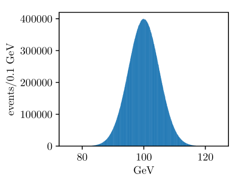
(a) $E_{\rm rec}$.

(b) $p_{\rm rec}$.

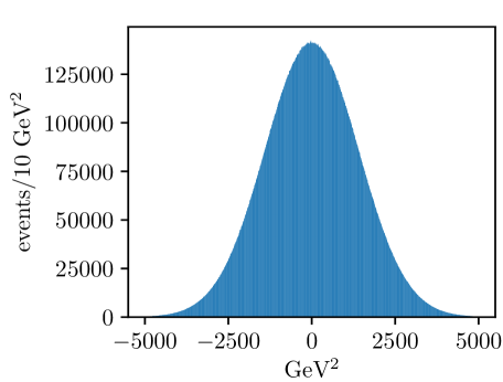
(c) $m^{2}_{\rm rec}$.

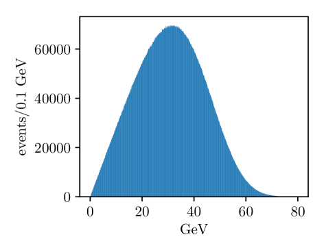
(d) $m_{\rm rec}$.

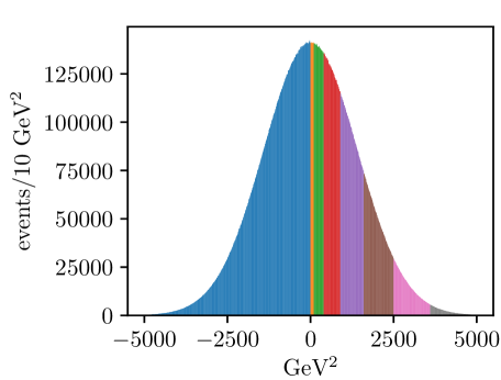
(e) Highlighted $m^{2}_{\rm rec}$.

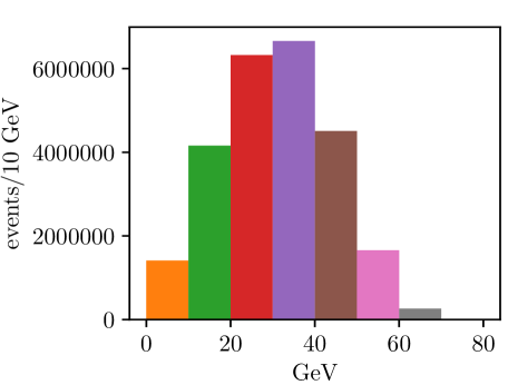
(f) Highlighted $m_{\rm rec}$.

Figure 11: Distributions of reconstructed values for $\varepsilon_{\rm E}=\varepsilon_{\rm p}=5\%$ and $E_{\rm beam}=100~{}\text{GeV}$.

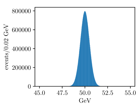
(a) $E_{\rm rec}$.

(b) $p_{\rm rec}$.

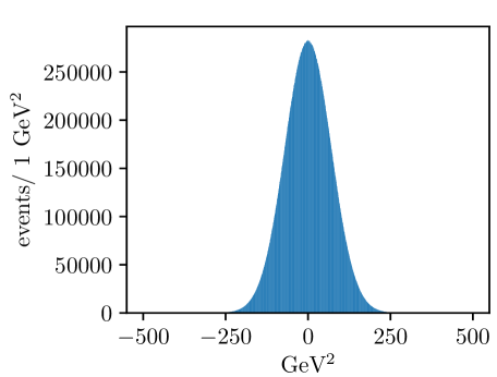
(c) $m^{2}_{\rm rec}$.

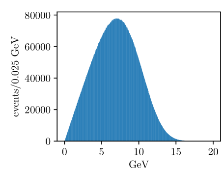
(d) $m_{\rm rec}$.

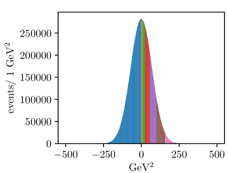
(e) Highlighted $m^{2}_{\rm rec}$.

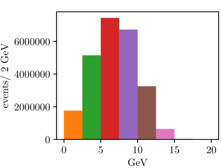
(f) Highlighted $m_{\rm rec}$.

Figure 12: Distributions of reconstructed values for $\varepsilon_{\rm E}=\varepsilon_{\rm p}=1\%$ and $E_{\rm beam}=50~{}\text{GeV}$.

References

- [1] E. Fermi. On the theory of the impact between atoms and electrically charged particles. Z.Physik 29, 315 (1924).
- [2] C. F. V. Weizsäcker. Radiation emitted in collisions of very fast electrons. Z.Physik 88, 612 (1934).
- [3] E. J. Williams. Correlation of certain collision problems with radiation theory. Kgl. Danske Vidensk. Selskab. Mat.-Fiz. Medd. 13, 4 (1935).
- [4] L. D. Landau, E. M. Lifshitz. Production of electrons and positrons by a collision of two particles. Phys.Zs.Sowjet 6, 244 (1934).
- [5] V. E. Balakin, V. M. Budnev, I. F. Ginzburg. Feasibility of an experiment in which hadrons are produced by two protons from threshold to extremely large energies. JETP Lett. 11, 388 (1970).
- [6] H. Terazawa. Two-photon processes for particle production at high energies. Rev.Mod.Phys. 4, 615 (1973).
- [7] V. M. Budnev, I. F. Ginzburg, G. V. Meledin, V. G. Serbo. The two-photon particle production and the equivalent photon approximation. Particles & Nuclei 4, 239 (1973) [in Russian].
- [8] V. M. Budnev, I. F. Ginzburg, G. V. Meledin, V. G. Serbo. The two-photon particle production mechanism. Physical problems. Applications. Equivalent photon approximation. Phys.Rep. 15, 181 (1975)
- [9] The ATLAS Collaboration. ATLAS Forward Proton Phase I Upgrade. Technical Design Report. CERN-LHCC-2015-009, ATLAS-TDR-024-2015.
- [10] The CMS and TOTEM Collaborations. CMS-TOTEM Precision Proton Spectrometer. Technical Design Report. CERN-LHCC-2014-021, TOTEM-TDR-003.
- [11] M. Albrow et al.. The FP420 R&D project: Higgs and New Physics with forward protons at the LHC. JINST 4, T10001 (2009). arXiv:0806.0302
- [12] M. Vysotsky, E. Zhemchugov. Equivalent photons in proton-proton and ion-ion collisions at the LHC. Physics-Uspekhi 189, 975 (2019). arXiv:1806.07238
- [13] J. Ohnemus, T. F. Walsh, P. M. Zerwas. production of non-strongly interacting SUSY particles at hadron colliders. Phys. Lett. B328, 369 (1994). arXiv:hep-ph/9402302
- [14] N. Schul, K. Piotrzkowski. Detection of two-photon exclusive production of supersymmetric pairs at the LHC. Nucl. Phys. Proc. Suppl. 179, 289 (2008). arXiv:0806.1097
- [15] V. A. Khoze, A. D. Martin, M. G. Ryskin, A. G. Shuvaev. A new window at the LHC: BSM signals using tagged protons. Eur. Phys. J. C68, 125 (2010). arXiv:1002.2857
- [16] L. A. Harland-Lang, C. H. Kom, K. Sakurai, W. J. Stirling. Measuring the masses of a pair of semi-invisibly decaying particles in central exclusive production with forward proton tagging. Eur. Phys. J. C72, 1969 (2012). arXiv:1110.4320
- [17] L. Beresford, J. Liu. Photon collider search strategy for sleptons and dark matter at the LHC. Phys. Rev. Lett. 123, 141801 (2019). arXiv:1811.06465
- [18] M. Tanabashi et al. (Particle Data Group). Review of Particle Physics. Phys. Rev. D98, 030001 (2018).
- [19] LEP2 SUSY Working Group, ALEPH, DELPHI, L3 and OPAL experiments. Combined LEP chargino results, up to 208 GeV for low DM. Note LEPSUSYWG/02-04.1 (2002), http://lepsusy.web.cern.ch/lepsusy
- [20] P. F. Smith, J. R. J. Bennett, G. J. Homer, J. D. Lewin, H. E. Walford, W. A. Smith. A search for anomalous hydrogen in enriched D2O, using a time-of-flight spectrometer. Nucl.Phys. B206, 333 (1982).
- [21] T. K. Hemmick, D. Elmore, T. Gentile, P. W. Kubik et al. Search for low- nuclei containing massive stable particles. Phys.Rev. D41, 2074 (1990).
- [22] P. Verkerk, G. Grynberg, B. Pichard, M. Spiro, S. Zylberajch, M. E. Goldberg, P. Fayet. Search for superheavy hydrogen in sea water. Phys.Rev.Lett. 68, 1116 (1992).
- [23] T. Yamagata, Y. Takamori, H. Utsunomiya. Search for anomalously heavy hydrogen in deep sea water at 4000 m. Phys.Rev. D47, 1231 (1993).
- [24] M. Byrne, Ch. Kolda, P. Regan. Bounds on charged, stable superpartners from cosmic ray production. Phys.Rev. D66, 075007 (2002). arXiv:hep-ph/0202252
- [25] The CMS Collaboration. Search for heavy stable charged particles in collisions at TeV. JHEP 1103, 024 (2011). arXiv:1101.1645
- [26] The ATLAS Collaboration. Search for heavy long-lived charged particles with the ATLAS detector in collisions at TeV. Phys. Lett. B703, 428 (2011). arXiv:1106.4495
- [27] The CMS Collaboration. Search for heavy long-lived charged particles in collisions at TeV. Phys. Lett. B713, 408 (2012). arXiv:1205.0272
- [28] The CMS Collaboration. Searches for long-lived charged particles in collisions at and 8 TeV. JHEP 1307, 122 (2013). arXiv:1305.0491
- [29] The ATLAS Collaboration. Searches for heavy long-lived particles with the ATLAS detector in proton-proton collisions at TeV. JHEP 1501, 068 (2015). arXiv:1411.6795
- [30] The CMS Collaboration. Constraints on the pMSSM, AMSB model and on other models from the search for long-lived charged particles in proton-proton collisions at TeV. Eur. Phys. J. C75, 325 (2015). arXiv:1502.02522
- [31] The ATLAS Collaboration. Search for metastable heavy charged particles with large ionization energy loss in collisions at TeV using the ATLAS experiment. Eur. Phys. J. C75, 407 (2015). arXiv:1506.05332
- [32] The LHCb Collaboration. Search for long-lived heavy charged particles using a ring imaging Cherenkov technique at LHCb. Eur. Phys. J. C75, 595 (2015). arXiv:1506.09173
- [33] The ATLAS Collaboration. Search for metastable heavy charged particles with large ionization energy loss in collisions at TeV using the ATLAS experiment. Phys. Rev. D93, 112015 (2016). arXiv:1604.04520
- [34] The CMS Collaboration. Search for long-lived charged particles in proton-proton collisions at TeV. Phys. Rev. D94, 112004 (2016). arXiv:1609.08382
- [35] The ATLAS Collaboration. Search for heavy charged long-lived particles in proton-proton collisions at TeV using an ionization measurement with the ATLAS detector. Phys. Lett. B788, 96 (2019). arXiv:1808.04095
- [36] The ATLAS Collaboration. Search for heavy charged long-lived particles in the ATLAS detector in of proton-proton collision data at TeV. Phys. Rev. D99, 092007 (2019). arXiv:1902.01636
- [37] V. B. Berestetskii, E. M. Lifshitz, L. P. Pitaevskii. Kvantovaya Electrodynamica. — Moscow: Fizmatlit, 2001.
- [38] S. Pacetti, R. B. Ferroli, E. Tomasi-Gustafsson. Proton electromagnetic form factors: basic notions, present achievements and future perspectives. Phys.Rep. 550, 1 (2015).
- [39] B. Dreher, J. Friedrech, K. Merle, H. Rothhaas, G. Lührs. The determination of the nuclear ground state and transition charge density from measured electron scattering data. Nucl.Phys. A235, 219 (1974).
- [40] H. de Vries, C. W. de Jager, C. de Vries. Nuclear charge-density-distribution parameters from elastic electron scattering. Atomic Data and Nuclear Data Tables 36, 495 (1987).
- [41] G. Breit, J. A. Wheeler. Collision of two light quanta. Phys.Rev. 46, 1087 (1934).
- [42] M. Dyndal, L. Schoeffel. The role of finite-size effects on the spectrum of equivalent photons in proton-proton collisions at the LHC. Phys. Lett. B741, 66 (2015). arXiv:1410.2983
- [43] L. A. Harland-Lang, V. A. Khoze, M. G. Ryskin. Exclusive physics at the LHC with SuperChic 2. Eur. Phys. J. C76, 9 (2016). arXiv:1508.02718
- [44] R. N. Cahn, J. D. Jackson. Realistic equivalent-photon yields in heavy-ion collisions. Phys. Rev. D42, 3690 (1990).
- [45] L. A. Harland-Lang, V. A. Khoze, M. G. Ryskin. Exclusive LHC physics with heavy ions: SuperChic 3. Eur. Phys. J. C79, 39 (2019). arXiv:1810.06567
-
[46]
ATLAS Luminosity—Public Results.
https://twiki.cern.ch/twiki/bin/view/AtlasPublic/LuminosityPublicResultsRun2 -
[47]
CMS Luminosity—Public Results.
https://twiki.cern.ch/twiki/bin/view/CMSPublic/LumiPublicResults - [48] The ATLAS Collaboration. Searches for electroweak production of supersymmetric particles with compressed mass spectra in TeV collisions with the ATLAS detector. ATLAS-CONF-2019-014 (2019).
- [49] The CMS Collaboration. Search for supersymmetry with a compressed mass spectrum in the vector boson fusion topology with 1-lepton and 0-lepton final states in proton-proton collisions at TeV. arXiv:1905.13059 (2019).
- [50] The ATLAS Collaboration. Search for long-lived charginos based on a disappearing-track signature in collisions at TeV with the ATLAS detector. JHEP 06, 022 (2018). arXiv:1712.02118
- [51] The CMS Collaboration. Search for disappearing tracks as a signature of new long-lived particles in proton-proton collisions at TeV. JHEP 1808, 016 (2018). arXiv:1804.07321
- [52] I. F. Ginzburg, G. L. Kotkin, S. L. Panfil, V. G. Serbo. boson production at the , and colliding beams. Nucl. Phys. B228, 285 (1983).
- [53] ATLAS Inner Detector Community. Technical Design Report vol. I. ATLAS-TDR-4, CERN/LHCC 97-16 (1997).
- [54] A. B. Kaidalov. Diffractive production mechanisms. Phys. Rep. 50, 157 (1979).
- [55] A. B. Kaidalov, V. A. Khoze, Yu. F. Pirogov, N. L. Ter-Isaakyan. On determination of the triple-pomeron coupling from the ISR data. Phys. Lett. B45, 493 (1973).
- [56] L. A. Harland-Lang, V. A. Khoze, M. G. Ryskin, M. Tasevsky. LHC searches for Dark Matter in compressed mass scenarios: challenges in the forward proton mode. JHEP 1904, 010 (2019). arXiv:1812.04886.
- [57] V. A. Khoze, A. D. Martin, M. G. Ryskin. Can invisible objects be ‘seen’ via forward proton detectors at the LHC? J. Phys. G44, 055002 (2017). arXiv:1702.05023.
- [58] The ATLAS Collaboration. Measurement of the exclusive process in proton-proton collisions at TeV with the ATLAS detector. Phys.Lett. B 777, 303 (2018). arXiv:1708.04053
- [59] R. Bruce, D. d’Enterria, A. de Roeck, M. Drewes et. al. New physics searches with heavy-ion collisions at the LHC. arXiv:1812.07688