Uniqueness in inverse electromagnetic scattering problem with phaseless far-field data at a fixed frequency

Abstract

This paper is concerned with uniqueness in inverse electromagnetic scattering with phaseless far-field pattern at a fixed frequency. In our previous work [SIAM J. Appl. Math. 78 (2018), 3024-3039], by adding a known reference ball into the acoustic scattering system, it was proved that the impenetrable obstacle and the index of refraction of an inhomogeneous medium can be uniquely determined by the acoustic phaseless far-field patterns generated by infinitely many sets of superpositions of two plane waves with different directions at a fixed frequency. In this paper, we extend these uniqueness results to the inverse electromagnetic scattering case. The phaseless far-field data are the modulus of the tangential component in the orientations $\bm{e}_{\phi}$ and $\bm{e}_{\theta}$, respectively, of the electric far-field pattern measured on the unit sphere and generated by infinitely many sets of superpositions of two electromagnetic plane waves with different directions and polarizations. Our proof is mainly based on Rellich’s lemma and the Stratton–Chu formula for radiating solutions to the Maxwell equations.

Keywords: Uniqueness, inverse electromagnetic scattering, phaseless far-field pattern, perfectly conducting obstacle, impedance obstacle, partially coated obstacle, inhomogeneous medium.

1 Introduction

Inverse scattering theory has wide applications in such fields as radar, sonar, geophysics, medical imaging, and nondestructive testing (see, e.g., [8, 15]). This paper is concerned with inverse electromagnetic scattering by a bounded obstacles or an inhomogeneous medium from phaseless far-field data, associated with incident plane waves at a fixed frequency.

Inverse scattering problems with phased data have been extensively studied both mathematically and numerically in the past several decades (see, e.g., [3, 8, 15]). However, in many applications, it is difficult to measure the phase of the wave field accurately, compared with the modulus of the wave field. Therefore, it is desirable to reconstruct the scatterers from the phaseless near-field or far-field data (i.e., the intensity of the near-field or far-field), which is called the phaseless inverse scattering problem.

The main difficulty of inverse scattering problems with phaseless far-field data is the so-called translation invariance property of the phaseless far-field pattern, that is, the modulus of the far-field pattern generated by one plane wave is invariant under the translation of the scatterers. This implies that it is impossible to recover the location of the scatterer from the phaseless far-field data with one plane wave as the incident field. Several iterative methods have been proposed in [12, 13, 14, 21] to reconstruct the shape of the scatterer. Under a priori condition that the sound-soft scatterer is a ball or disk, it was proved in [22] that the radius of the scatterer can be uniquely determined by a single phaseless far-field datum. It was proved in [23] that the shape of a general, sound-soft, strictly convex obstacle can be uniquely determined by the phaseless far-field data generated by one plane wave at a high frequency. However, there is no translation invariance property for phaseless near-field data. Therefore, many numerical algorithms for inverse scattering problems with phaseless near-field data have been developed (see, e.g., [3, 4, 6, 18, 32, 36] for the acoustic case and [5] for the electromagnetic case). Uniqueness results and stability have also been established for inverse scattering problems with phaseless near-field data (see [16, 17, 19, 24, 26, 27, 30, 37, 42, 43] for the acoustic and potential scattering case and [29, 37] for the electromagnetic scattering case).

Recently in [38], it was proved that the translation invariance property of the phaseless far-field pattern can be broken by using superpositions of two plane waves as the incident fields with an interval of frequencies. Following this idea, several algorithms have been developed for inverse acoustic scattering problems with phaseless far-field data, based on using the superposition of two plane waves as the incident field (see [38, 39, 40]). Further, by using the spectral properties of the far-field operator, rigorous uniqueness results have also been established in [34] for inverse acoustic scattering problems with phaseless far-field data generated by infinitely many sets of superpositions of two plane waves with different directions at a fixed frequency, under certain a priori assumptions on the property of the scatterers. In [35], by adding a known reference ball into the acoustic scattering system, it was shown that the uniqueness results obtained in [34] remain true without the a priori assumptions on the property of the scatterers. Note that the idea of adding a known reference ball to the scattering system was first applied in [11] to numerically enhance the reconstruction results of the linear sampling method and also used in [41] to prove uniqueness in inverse acoustic scattering problems with phaseless far-field data. Note further that there are certain studies on uniqueness for phaseless inverse scattering problems with using superpositions of two point sources as the incident fields (see [30, 33, 37, 42, 43]).

The purpose of this paper is to establish uniqueness results in inverse electromagnetic scattering problems with phaseless far-field data at a fixed frequency, extending the uniqueness results in [35] for the acoustic case to the electromagnetic case. Different from the acoustic case considered in [35], the electric far-field pattern is a complex-valued vector function, so the measurement of the phaseless electric far-field pattern is more complicated. In practice, one usually makes measurement of the modulus of each tangential component of the electric total-field or electric far-field pattern on the measurement surface (see, e.g., [10, 28, 31, 44]). Motivated by this and the idea in [34, 35], we make use of superpositions of two electromagnetic plane waves with different directions and polarizations as the incident fields and consider the modulus of the tangential component in the orientations $\bm{e}_{\phi}$ and $\bm{e}_{\theta}$, respectively, of the corresponding electric far-field pattern measured on the unit sphere as the measurement data (called the phaseless electric far-field data). We then prove that, by adding a known reference ball into the electromagnetic scattering system, the impenetrable obstacle or the refractive index of the inhomogeneous medium (under the condition that the magnetic permeability is a positive constant) can be uniquely determined by the phaseless electric far-field data at a fixed frequency. Our proof is mainly based on Rellich’s lemma and the Stratton–Chu formula for radiating solutions to the Maxwell equations.

The rest part of this paper is organised as follows. In Section 2, we introduce the electromagnetic scattering problems considered. The uniqueness results for inverse obstacle and medium electromagnetic scattering with phaseless electric far-field data are presented in Section 3 and 4, respectively. Conclusions are given in Section 5.

2 The electromagnetic scattering problems

In this section, we introduce the electromagnetic scattering problems considered in this paper. To give a precise description of the scattering problems, we assume that $D$ is an open and bounded domain in ${\mathbb{R}}^{3}$ with $C^{2}-$boundary $\partial D$ satisfying that the exterior ${\mathbb{R}}^{3}\setminus\overline{D}$ of $D$ is connected. Note that $D$ may not be connected and thus may consist of several (finitely many) connected components. We consider the time-harmonic ($e^{-i\omega t}$ time dependence) incident electromagnetic plane waves described by the matrices $E^{i}(x,d)$ and $H^{i}(x,d)$ defined by

$$E^{i}(x,d)p:=\frac{i}{k}{\rm curl}\,{\rm curl}\,pe^{ikx\cdot d}=ik(d\times p)\times de^{ikx\cdot d},\quad x\in{\mathbb{R}}^{3},$$ (2.1)

$$H^{i}(x,d)p:={\rm curl}\,pe^{ikx\cdot d}=ikd\times pe^{ikx\cdot d},\quad x\in{\mathbb{R}}^{3},$$ (2.2)

where $d\in{\mathbb{S}}^{2}$ is the incident direction with ${\mathbb{S}}^{2}$ being the unit sphere, $p\in{\mathbb{R}}^{3}$ is the polarization vector, $k=\omega/\sqrt{\varepsilon_{0}\mu_{0}}$ is the wave number, $\omega$ is the frequency, and $\varepsilon_{0}$ and $\mu_{0}$ are the electric permittivity and magnetic permeability of a homogeneous medium, respectively.

When $D$ is an impenetrable obstacle, then the scattering problem can be modeled by the exterior boundary value problem:

$${\rm curl}\,E-ikH=0 \;\;\text{in}\;\;{\mathbb{R}}^{3}\setminus\overline{D},$$ (2.3a)

$${\rm curl}\,H+ikE=0 \;\;\text{in}\;\;{\mathbb{R}}^{3}\setminus\overline{D},$$ (2.3b)

$$\mathscr{B}E=0 \;\;\text{on}\;\;\partial D,$$ (2.3c)

$$\lim_{r\rightarrow\infty}(H^{s}\times x-rE^{s})=0, \;\;r=|x|,$$ (2.3d)

where $(E^{s},H^{s})$ is the scattered field, $E:=E^{i}+E^{s}$ and $H:=H^{i}+H^{s}$ are the electric total-field and the magnetic total-field, respectively, the equations (2.3a)–(2.3b) are the Maxwell equations, and (2.3d) is the Silver–Müller radiation condition. The boundary condition $\mathscr{B}$ in (2.3c) depends on the physical property of the obstacle $D$, that is, $\mathscr{B}E=\nu\times E$ if $D$ is a perfectly conducting obstacle, $\mathscr{B}E=\nu\times{\rm curl\,}{E}-i\lambda(\nu\times E)\times\nu=0$ if $D$ is an impedance obstacle, and $\mathscr{B}E=\nu\times E$ on $\Gamma_{D}$, $\mathscr{B}E=\nu\times{\rm curl\,}{E}-i\lambda(\nu\times E)\times\nu=0$ on $\Gamma_{I}$ if $D$ is a partially coated obstacle, where $\nu$ is the unit outward normal vector on the boundary $\partial D$. Here, for the case when $D$ is an impedance obstacle, we assume that $\lambda$ is the impedance function on $\partial D$ with $\lambda\in C(\partial D)$ and $\lambda(x)\geq 0$ for all $x\in\partial D$. Further, for the case when $D$ is a partially coated obstacle, we assume that $\partial D$ has a Lipschitz dissection $\partial D=\Gamma_{D}\cup\Pi\cup\Gamma_{I}$ with $\Gamma_{D}$ and $\Gamma_{I}$ being disjoint and relatively open subsets of $\partial D$ and having $\Pi$ as their common boundary in $\partial D$ (see, e.g. [25]) and $\lambda$ is the impedance function on $\Gamma_{I}$ with $\lambda\in C(\Gamma_{I})$ and $\lambda(x)\geq 0$ for all $x\in\Gamma_{I}$.

When $D$ is an inhomogeneous medium, we assume that the magnetic permeability $\mu=\mu_{0}$ is a positive constant in the whole space. Then the scattering problem is modeled by the medium scattering problem

$${\rm curl}\,E-ikH=0 \;\;\text{in}\;\;{\mathbb{R}}^{3},$$ (2.4a)

$${\rm curl}\,H+iknE=0 \;\;\text{in}\;\;{\mathbb{R}}^{3},$$ (2.4b)

$$\lim_{r\rightarrow\infty}(H^{s}\times x-rE^{s})=0, \;\;r=|x|,$$ (2.4c)

where $(E^{s},H^{s})$ is the scattered field, $E:=E^{i}+E^{s}$ and $H:=H^{i}+H^{s}$ are the electric total-field and the magnetic total-field, respectively. The refractive index $n$ in (2.4b) is given by

$$n(x):=\frac{1}{\varepsilon_{0}}\left(\varepsilon(x)+i\frac{\sigma(x)}{\omega}\right),$$

where $\varepsilon(x)$ is the electric permittivity with $\varepsilon(x)\geq\varepsilon_{min}$ in ${\mathbb{R}}^{3}$ for a constant $\varepsilon_{min}>0$ and $\sigma(x)$ is the electric conductivity with $\sigma(x)\geq 0$ in ${\mathbb{R}}^{3}$. We assume further that $n-1$ has a compact support $\overline{D}$ and $n\in C^{2,\gamma}({\mathbb{R}}^{3})$ for $0<\gamma<1$. From the above assumptions, it can be seen that ${\rm Re}[n(x)]\geq n_{min}:=\varepsilon_{min}/\varepsilon_{0}>0$ and ${\rm Im}[n(x)]\geq 0$ for all $x\in{\mathbb{R}}^{3}$.

The existence of a unique (variational) solution to the problems (2.3a)–(2.3d) and (2.4a)–(2.4c) has been proved in [1, 2, 7, 8, 25] (see Theorem 6.21 in [8] and Theorem 10.8 in [25] for scattering by a perfectly conducting obstacle or an impedance obstacle with $\lambda\equiv 0$ on $\partial D$, Theorems 6.11 and 9.11 in [8] for scattering by an impedance obstacle with constant impedance function, Theorems 2.1 and 3.3 in [7] for scattering by an impedance obstacle with $\lambda\in C^{0,\gamma}(\partial D)$, Theorem 3.5 in [2] (see also Theorem 2.7 in [1]) for scattering by a partly coated obstacle or an impedance obstacle and Theorem 5.5 in [15] (see also Theorem 9.5 in [8]) for scattering by an inhomogeneous medium). In particular, it is well-known from [8] that the electric and magnetic scattered fields $E^{s}$ and $H^{s}$ have the asymptotic behavior

$$E^{s}(x,d)p=\frac{e^{ik|x|}}{|x|}\left\{E^{\infty}(\hat{x},d)p+O\left(\frac{1}{|x|}\right)\right\},\;\;|x|\rightarrow\infty,$$

$$H^{s}(x,d)p=\frac{e^{ik|x|}}{|x|}\left\{H^{\infty}(\hat{x},d)p+O\left(\frac{1}{|x|}\right)\right\},\;\;|x|\rightarrow\infty$$

uniformly for all observation directions $\hat{x}=x/|x|\in{\mathbb{S}}^{2}$, where $E^{\infty}(\hat{x},d)p$ is the electric far-field pattern of $E^{s}(x,d)p$ and $H^{\infty}(\hat{x},d)p$ is the magnetic far-field pattern of $H^{s}(x,d)p$ for any $p\in{\mathbb{R}}^{3}$, satisfying that (see [8, (6.24)])

$$H^{\infty}(\hat{x},d)p=\hat{x}\times E^{\infty}(\hat{x},d)p,\;\;\;\hat{x}\cdot E^{\infty}(\hat{x},d)p=\hat{x}\cdot H^{\infty}(\hat{x},d)p=0.$$ (2.5)

Because of the linearity of the direct scattering problem with respect to the incident field, the scattered waves, the total-fields and the corresponding far-field patterns can be represented by matrices $E^{s}(x,d)$ and $H^{s}(x,d)$, $E(x,d)$ and $H(x,d)$, and $E^{\infty}(\hat{x},d)$ and $H^{\infty}(\hat{x},d)$, respectively. Each component of the matrices $E^{\infty}(\hat{x},d)$ and $H^{\infty}(\hat{x},d)$ is an analytic function of $\hat{x}\in{\mathbb{S}}^{2}$ for each $d\in{\mathbb{S}}^{2}$ and of $d\in{\mathbb{S}}^{2}$ for each $\hat{x}\in{\mathbb{S}}^{2}$ (see, e.g., [8]).

Throughout this paper, we assume that the wave number $k$ is arbitrarily fixed, i.e., the frequency $\omega$ is arbitrarily fixed. Following [34, 35, 38, 39], we make use of the following superposition of two plane waves as the incident (electric) field:

$$E^{i}:=E^{i}(x,d_{1},d_{2},p_{1},p_{2})=E^{i}(x,d_{1})p_{1}+E^{i}(x,d_{2})p_{2}=\frac{i}{k}{\rm curl}\,{\rm curl}\,p_{1}e^{ikx\cdot d_{1}}+\frac{i}{k}{\rm curl}\,{\rm curl}\,p_{2}e^{ikx\cdot d_{2}},$$

where $d_{1},d_{2}\in{\mathbb{S}}^{2}$ and $p_{1},p_{2}\in{\mathbb{R}}^{3}$. Then the (electric) scattered field $E^{s}$ has the asymptotic behavior

$$E^{s}(x,d_{1},d_{2},p_{1},p_{2})=\frac{e^{ik|x|}}{|x|}\left\{E^{\infty}(\hat{x},d_{1},d_{2},p_{1},p_{2})+O\left(\frac{1}{|x|}\right)\right\},\;|x|\rightarrow\infty$$

uniformly for all observation directions $\hat{x}\in{\mathbb{S}}^{2}$. From the linear superposition principle it follows that

$$E^{s}(x,d_{1},d_{2},p_{1},p_{2})=E^{s}(x,d_{1})p_{1}+E^{s}(x,d_{2})p_{2}$$

and

$$E^{\infty}(\hat{x},d_{1},d_{2},p_{1},p_{2})=E^{\infty}(\hat{x},d_{1})p_{1}+E^{\infty}(\hat{x},d_{2})p_{2},$$ (2.6)

where $E^{s}(x,d_{j})p_{j}$ and $E^{\infty}(\hat{x},d_{j})p_{j}$ are the (electric) scattered field and its far-field pattern corresponding to the incident electric field $E^{i}(x,d_{j})p_{j}$, respectively, $j=1,2$.

Following the idea in [10, 28, 31, 44], we measure the modulus of the tangential component of the electric far-field pattern on the unit sphere ${\mathbb{S}}^{2}$. To present the tangential components, we introduce the spherical coordinates

$$\begin{cases}\hat{x}_{1}=\sin\theta\cos\phi,\\ \hat{x}_{2}=\sin\theta\sin\phi,\\ \hat{x}_{3}=\cos\theta,\end{cases}$$

with $\hat{x}:=(\hat{x}_{1},\hat{x}_{2},\hat{x}_{3})\in{\mathbb{S}}^{2}$ and $(\theta,\phi)\in[0,\pi]\times[0,2\pi)$. For any $\hat{x}\in{\mathbb{S}}^{2}\setminus\{N,S\}$, the spherical coordinates give an one-to-one correspondence between $\hat{x}$ and $(\phi,\theta)$, where $N:=(0,0,1)$ and $S:=(0,0,-1)$ denote the north and south poles of ${\mathbb{S}}^{2}$, respectively. Define

$$\bm{e}_{\phi}(\hat{x}):=(-\sin\phi,\cos\phi,0),\;\;\;\;\bm{e}_{\theta}(\hat{x}):=(\cos\theta\cos\phi,\cos\theta\sin\phi,-\sin\theta).$$

Then $\bm{e}_{\phi}(\hat{x})$ and $\bm{e}_{\theta}(\hat{x})$ are two orthonormal tangential vectors of ${\mathbb{S}}^{2}$ at $\hat{x}\notin\{N,S\}$. Thus the phaseless far-field data we use are $|\bm{e}_{m}(\hat{x})\cdot E^{\infty}(\hat{x},d_{1},d_{2},p_{1},p_{2})|$, $\hat{x}\in{\mathbb{S}}^{2}\setminus\{N,S\}$, $m\in\{\phi,\theta\}$, $d_{j}\in{\mathbb{S}}^{2}$ and $p_{j}\in{\mathbb{R}}^{3}$ such that $d_{j}\bot p_{j}$, $j=1,2$.

The inverse electromagnetic obstacle (or medium) scattering problem we consider in this paper is to reconstruct the obstacle $D$ and its physical property (or the refractive index $n$ of the inhomogeneous medium) from the phaseless far-field data $|\bm{e}_{m}(\hat{x})\cdot E^{\infty}(\hat{x},d_{1},d_{2},p_{1},p_{2})|$, $\hat{x}\in{\mathbb{S}}^{2}\setminus\{N,S\}$, $m\in\{\phi,\theta\}$, $d_{j}\in{\mathbb{S}}^{2}$ and $p_{j}\in{\mathbb{R}}^{3}$ such that $d_{j}\bot p_{j}$, $j=1,2$. The purpose of this paper is to establish the uniqueness results for these inverse problems.

3 Uniqueness for inverse electromagnetic obstacle scattering

Let $B$ be a given, perfectly conducting ball and let us assume that $k$ is not a Maxwell eigenvalue in $B$. Here, $k$ is called a Maxwell eigenvalue in $B$ if the electromagnetic interior boundary value problem

$${\rm curl}\,\widetilde{E}-ik\widetilde{H}=0 \text{in}\;\;B,$$ (3.1)

$${\rm curl}\,\widetilde{H}+ik\widetilde{E}=0 \text{in}\;\;B,$$ (3.2)

$$\nu\times\widetilde{E}=0 \text{on}\;\;\partial B$$ (3.3)

has a nontrivial solution $(\widetilde{E},\widetilde{H})$. Note that, if the radius $r$ of the ball $B$ is chosen so that $j_{n}(kr)\neq 0$ and $j_{n}(kr)+krj^{\prime}_{n}(kr)\neq 0$ for $n=0,1,\ldots$, then $k$ is not a Maxwell eigenvalue in $B$ (see [8, Page 252]), where $j_{n}$ denotes the spherical Bessel function of order $n$.

Now, denote by $E_{j}^{s}$, $H_{j}^{s}$, $E_{j}^{\infty}$, and $H_{j}^{\infty}$ the electric scattered field, the magnetic scattered field, the electric far-field pattern and the magnetic far-field pattern, respectively, associated with the obstacle $D_{j}\cup B$ and corresponding to the incident electromagnetic waves $E^{i}$ and $H^{i}$, $j=1,2$. The geometry of the scattering problem is given in Figure 1. Then we have the following uniqueness result for the inverse electromagnetic obstacle problem.

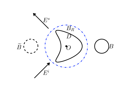
Figure 1: Scattering by a bounded obstacle.

Theorem 3.1.

Assume that $B$ is a given perfectly conducting reference ball such that $k$ is not a Maxwell eigenvalue in $B$. Suppose $D_{1}$ and $D_{2}$ are two obstacles with $\overline{D_{1}\cup D_{2}}\subset B_{R}$, where $B_{R}$ is a ball of radius $R$ and centered at the origin satisfying that $\overline{B}\cap\overline{B_{R}}=\emptyset$. If the corresponding electric far-field patterns satisfy that

$$|\bm{e}_{m}(\hat{x})\cdot E_{1}^{\infty}(\hat{x},d_{1},d_{2},p_{1},p_{2})|=|\bm{e}_{m}(\hat{x})\cdot E_{2}^{\infty}(\hat{x},d_{1},d_{2},p_{1},p_{2})|$$ (3.4)

for all $\hat{x}\in{\mathbb{S}}^{2}\setminus\{N,S\}$, $d_{1},d_{2}\in{\mathbb{S}}^{2}$, $m\in\{\phi,\theta\}$ and $p_{1},p_{2}\in{\mathbb{R}}^{3}$ satisfying that $d_{1}\bot p_{1}$ and $d_{2}\bot p_{2}$, then $D_{1}=D_{2}$ and $\mathscr{B}_{1}=\mathscr{B}_{2}$.

To prove Theorem 3.1, we need the following lemma.

Lemma 3.2.

Under the assumptions of Theorem 3.1, the following equation does not hold:

$$E_{1}^{\infty}(\hat{x},d_{0})\bm{e}_{m}(d_{0})=e^{i\beta}\overline{E_{2}^{\infty}(\hat{x},d_{0})}\bm{e}_{m}(d_{0})\;\;\;\forall\hat{x}\in{\mathbb{S}}^{2},$$ (3.5)

where $m\in\{\phi,\theta\}$ and $d_{0}\in{\mathbb{S}}^{2}\setminus\{N,S\}$ are arbitrarily fixed and $\beta$ is a real constant.

Proof.

Assume to the contrary that (3.5) holds. Then, by using the Stratton–Chu formula (see [8, Theorem 6.7]), we have that the electric scattered field $E_{2}^{s}(x,d_{0})\bm{e}_{m}(d_{0})$ satisfies that

$$E_{2}^{s}(x,d_{0})\bm{e}_{m}(d_{0}) = {\rm curl}\,\int_{\partial B\cup\partial B_{R}}\nu(y)\times[E_{2}^{s}(y,d_{0})\bm{e}_{m}(d_{0})]\Phi(x,y)ds(y)$$

$$-\frac{1}{ik}{\rm curl}\,{\rm curl}\,\int_{\partial B\cup\partial B_{R}}\nu(y)\times[H_{2}^{s}(y,d_{0})\bm{e}_{m}(d_{0})]\Phi(x,y)ds(y),\;x\in{\mathbb{R}}^{3}\setminus\overline{B\cup B_{R}},$$

where $\nu(y)$ is the unit normal vector at $y\in\partial B$ or $y\in\partial B_{R}$ directed into the exterior of $B$ or $B_{R}$ and $\Phi(x,y)$ is the fundamental solution to the Helmholtz equation in ${\mathbb{R}}^{3}$ given by

$$\Phi(x,y):=\frac{1}{4\pi}\frac{e^{ik|x-y|}}{|x-y|},\;\;\;x\neq y.$$

Then it follows from [8, (6.25)] that the corresponding far-field pattern $E_{2}^{\infty}(\hat{x},d_{0})\bm{e}_{m}(d_{0})$ is given as

$$E_{2}^{\infty}(\hat{x},d_{0})\bm{e}_{m}(d_{0})$$

$$\quad=\frac{ik}{4\pi}\hat{x}\times\int_{\partial B\cup\partial B_{R}}\left\{\nu(y)\times[E_{2}^{s}(y,d_{0})\bm{e}_{m}(d_{0})]+\left[\nu(y)\times[H_{2}^{s}(y,d_{0})\bm{e}_{m}(d_{0})]\right]\times\hat{x}\right\}e^{-ik\hat{x}\cdot y}ds(y),\;\;\hat{x}\in{\mathbb{S}}^{2}.\qquad$$

By this and (3.5) we deduce that for any $\hat{x}\in{\mathbb{S}}^{2}$,

$$e^{-i\beta}E_{1}^{\infty}(\hat{x},d_{0})\bm{e}_{m}(d_{0})=\overline{E_{2}^{\infty}(\hat{x},d_{0})}\bm{e}_{m}(d_{0})$$

$$\;=-\frac{ik}{4\pi}\hat{x}\times\int_{\partial B\cup\partial B_{R}}\left\{\nu(y)\times[\overline{E_{2}^{s}(y,d_{0})}\bm{e}_{m}(d_{0})]+\left[\nu(y)\times[\overline{H_{2}^{s}(y,d_{0})}\bm{e}_{m}(d_{0})]\right]\times\hat{x}\right\}e^{ik\hat{x}\cdot y}ds(y)$$

$$\;=-\frac{ik}{4\pi}\hat{x}\times\int_{\partial\widetilde{B}\cup\partial B_{R}}\left\{-\nu(y)\times[\overline{E_{2}^{s}(-y,d_{0})}\bm{e}_{m}(d_{0})]+\left[-\nu(y)\times[\overline{H_{2}^{s}(-y,d_{0})}\bm{e}_{m}(d_{0})]\right]\times\hat{x}\right\}e^{-ik\hat{x}\cdot y}ds(y)$$

$$\;=\frac{ik}{4\pi}\hat{x}\times\int_{\partial\widetilde{B}\cup\partial B_{R}}\left\{\nu(y)\times[\overline{E_{2}^{s}(-y,d_{0})}\bm{e}_{m}(d_{0})]+\left[\nu(y)\times[\overline{H_{2}^{s}(-y,d_{0})}\bm{e}_{m}(d_{0})]\right]\times\hat{x}\right\}e^{-ik\hat{x}\cdot y}ds(y),\quad$$

where $\widetilde{B}:=\{x\in{\mathbb{R}}^{3}:-x\in B\}$. Then, by Rellich’s lemma we have

$$e^{-i\beta}E_{1}^{s}(x,d_{0})\bm{e}_{m}(d_{0}) = {\rm curl}\,\int_{\partial\widetilde{B}\cup\partial B_{R}}\nu(y)\times[\overline{E_{2}^{s}(-y,d_{0})}\bm{e}_{m}(d_{0})]\Phi(x,y)ds(y)$$

$$-\frac{1}{ik}{\rm curl}\,{\rm curl}\,\int_{\partial\widetilde{B}\cup\partial B_{R}}\nu(y)\times[\overline{H_{2}^{s}(-y,d_{0})}\bm{e}_{m}(d_{0})]\Phi(x,y)ds(y),\;x\in{\mathbb{R}}^{3}\setminus\overline{\widetilde{B}\cup B_{R}}.$$

This implies that $E_{1}^{s}(\cdot,d_{0})\bm{e}_{m}(d_{0})$ can be analytically extended into ${\mathbb{R}}^{3}\setminus\overline{\widetilde{B}\cup B_{R}}$. Since

$$H_{1}^{s}(\cdot,d_{0})\bm{e}_{m}(d_{0})=\frac{1}{ik}{\rm curl}\,[E_{1}^{s}(\cdot,d_{0})\bm{e}_{m}(d_{0})],$$

then it follows from (3) that $E_{1}^{s}(\cdot,d_{0})\bm{e}_{m}(d_{0})$ and $H_{1}^{s}(\cdot,d_{0})\bm{e}_{m}(d_{0})$ satisfy the Maxwell equations (2.3a)–(2.3b) in ${\mathbb{R}}^{3}\setminus\overline{\widetilde{B}\cup B_{R}}$. On the other hand, by the definitions of $E^{s}_{1}$ and $H^{s}_{1}$ it is known that $E_{1}^{s}(\cdot,d_{0})\bm{e}_{m}(d_{0})$ and $H_{1}^{s}(\cdot,d_{0})\bm{e}_{m}(d_{0})$ also satisfy the Maxwell equations (2.3a)–(2.3b) in ${\mathbb{R}}^{3}\setminus\overline{B\cup B_{R}}$. Since $\overline{B}\cap\overline{B_{R}}=\emptyset$, then the origin $0\notin B$ and $B\cap\widetilde{B}=\emptyset$. Thus it is concluded that $E_{1}^{s}(\cdot,d_{0})\bm{e}_{m}(d_{0})$ and $H_{1}^{s}(\cdot,d_{0})\bm{e}_{m}(d_{0})$ satisfy the Maxwell equations (2.3a)–(2.3b) in ${\mathbb{R}}^{3}\setminus\overline{B_{R}}$. Since the electric total field $E_{1}:=E_{1}(\cdot,d_{0})\bm{e}_{m}(d_{0})=E_{1}^{i}(\cdot,d_{0})\bm{e}_{m}(d_{0})+E_{1}^{s}(\cdot,d_{0})\bm{e}_{m}(d_{0})$ and the magnetic total field $H_{1}:=(1/{ik}){\rm curl\,}\,E_{1}$ satisfy the perfectly conducting boundary condition on $\partial B$, then $(E_{1},H_{1})$ satisfies the problem (3.1)–(3.3). By the fact that $k$ is not a Maxwell eigenvalue in $B$ we have that $E_{1}\equiv 0$ in $B$, which, together with the analyticity of the electric total field $E_{1}$ in ${\mathbb{R}}^{3}\setminus\overline{B_{R}}$, implies that $E_{1}\equiv 0$ in ${\mathbb{R}}^{3}\setminus\overline{B_{R}}$. This is a contradiction, and so (3.5) dose not hold. The proof is complete. ∎

We are now ready to prove Theorem 3.1.

Proof of Theorem 3.1.

Using (2.6) and (3.4), we have

$$|\bm{e}_{m}(\hat{x})\cdot[E_{1}^{\infty}(\hat{x},d_{1})p_{1}+E_{1}^{\infty}(\hat{x},d_{2})p_{2}]|=|\bm{e}_{m}(\hat{x})\cdot[E_{2}^{\infty}(\hat{x},d_{1})p_{1}+E_{2}^{\infty}(\hat{x},d_{2})p_{2}|$$ (3.7)

for all $\hat{x}\in{\mathbb{S}}^{2}\setminus\{N,S\}$, $d_{1},d_{2}\in{\mathbb{S}}^{2}$, $m\in\{\phi,\theta\}$ and $p_{1},p_{2}\in{\mathbb{R}}^{3}$ satisfying that $d_{1}\bot p_{1}$ and $d_{2}\bot p_{2}$. By (2.1) we know that $E^{i}(x,d)d=0$ for all $\hat{x},d\in{\mathbb{S}}^{2}$, and so, from the well-posedness of the scattering problem it follows that

$$E_{j}^{\infty}(\hat{x},d)d=0\;\;\;\forall\hat{x},d\in{\mathbb{S}}^{2}.$$ (3.8)

Thus (3.7) is equivalent to the condition

$$|\bm{e}_{m}(\hat{x})\cdot[E_{1}^{\infty}(\hat{x},d_{1})p_{1}+E_{1}^{\infty}(\hat{x},d_{2})p_{2}]|=|\bm{e}_{m}(\hat{x})\cdot[E_{2}^{\infty}(\hat{x},d_{1})p_{1}+E_{2}^{\infty}(\hat{x},d_{2})p_{2}|$$ (3.9)

for all $\hat{x}\in{\mathbb{S}}^{2}\setminus\{N,S\}$, $d_{1},d_{2}\in{\mathbb{S}}^{2}$, $m\in\{\phi,\theta\}$ and $p_{1},p_{2}\in{\mathbb{R}}^{3}$. This implies that

$${\rm Re}\left\{[\bm{e}_{m}(\hat{x})\cdot E_{1}^{\infty}(\hat{x},d_{1})p_{1}]\times\overline{[\bm{e}_{m}(\hat{x})\cdot E_{1}^{\infty}(\hat{x},d_{2})p_{2}]}\right\}$$

$$\qquad\qquad={\rm Re}\left\{[\bm{e}_{m}(\hat{x})\cdot E_{2}^{\infty}(\hat{x},d_{1})p_{2}]\times\overline{[\bm{e}_{m}(\hat{x})\cdot E_{2}^{\infty}(\hat{x},d_{2})p_{2}]}\right\}$$ (3.10)

for all $\hat{x}\in{\mathbb{S}}^{2}\setminus\{N,S\}$, $d_{1},d_{2}\in{\mathbb{S}}^{2}$, $m\in\{\phi,\theta\}$ and $p_{1},p_{2}\in{\mathbb{R}}^{3}$.

For $d,q\in{\mathbb{S}}^{2}$ and $p\in{\mathbb{R}}^{3}$ define $r_{j}(\hat{x},d,q,p):=|q\cdot E_{j}^{\infty}(\hat{x},d)p|,\;j=1,2$. Then, by setting $d_{1}=d_{2}=:d$ and $p_{1}=p_{2}=:p$ in (3.9) we have

$$r_{1}(\hat{x},d,\bm{e}_{m}(\hat{x}),p) = r_{2}(\hat{x},d,\bm{e}_{m}(\hat{x}),p)=:r(\hat{x},d,\bm{e}_{m}(\hat{x}),p)$$ (3.11)

$$\qquad\;\forall\hat{x}\in{\mathbb{S}}^{2}\setminus\{N,S\},\;d\in{\mathbb{S}}^{2},\;m\in\{\phi,\theta\},\;p\in{\mathbb{R}}^{3}.$$

Thus we know that

$$\bm{e}_{m}(\hat{x})\cdot E_{j}^{\infty}(\hat{x},d)p=r(\hat{x},d,\bm{e}_{m}(\hat{x}),p)e^{i\vartheta_{j}^{(m)}(\hat{x},d,p)}\;\;\;\forall\hat{x}\in{\mathbb{S}}^{2}\setminus\{N,S\},\;d\in{\mathbb{S}}^{2},\;m\in\{\phi,\theta\},\;p\in{\mathbb{R}}^{3},j=1,2,$$

where $\vartheta_{j}^{(m)}$ is a real-valued function, $j=1,2$.

Let $m\in\{\phi,\theta\}$ be arbitrarily fixed. We then prove that

$$E_{1}^{\infty}(\hat{x},d)\bm{e}_{m}(d)=E_{2}^{\infty}(\hat{x},d)\bm{e}_{m}(d)\;\;\;\forall\hat{x}\in{\mathbb{S}}^{2},\;d\in{\mathbb{S}}^{2}\setminus\{N,S\}.$$ (3.12)

To do this, we distinguish between the following two cases.

Case 1. $r(\hat{x},d,\bm{e}_{m}(\hat{x}),p)\not\equiv 0$ for $\hat{x}\in{\mathbb{S}}^{2}\setminus\{N,S\}$, $d\in{\mathbb{S}}^{2}$ and $p\in{\mathbb{R}}^{3}$.

In this case, by the analyticity of $\bm{e}_{m}(\hat{x})\cdot E_{j}^{\infty}(\hat{x},d)p$ with respect to $\hat{x}$, $d$ and $p$, respectively, $j=1,2$, it is easily seen that there exist open sets $U_{1}\subset{\mathbb{S}}^{2}\setminus\{N,S\}$, $U_{2}\subset{\mathbb{S}}^{2}$ and $V\subset{\mathbb{R}}^{3}$ small enough such that (i) $r(\hat{x},d,\bm{e}_{m}(\hat{x}),p)\not=0$ for all $\hat{x}\in U_{1}$, $d\in U_{2}$ and $p\in V$, and (ii) $\vartheta_{j}^{(m)}(\hat{x},d,p)$ is analytic with respect to $\hat{x}\in U_{1}$, $d\in U_{2}$ and $p\in V$, respectively, $j=1,2$. Then, and by (3.10) we obtain that

$$\cos[\vartheta_{1}^{(m)}(\hat{x},d_{1},p_{1})-\vartheta_{1}^{(m)}(\hat{x},d_{2},p_{2})]=\cos[\vartheta_{2}^{(m)}(\hat{x},d_{1},p_{1})-\vartheta_{2}^{(m)}(\hat{x},d_{2},p_{2})]$$ (3.13)

for all $\hat{x}\in U_{1}$, $d_{1},d_{2}\in U_{2}$ and $p_{1},p_{2}\in V$. From (3.13) and the fact that $\vartheta_{j}^{(m)}(\hat{x},d,p)$ is a real-valued analytic function of $\hat{x}\in U_{1}$, $d\in U_{2}$ and $p\in V$, respectively, $j=1,2$, it is derived that there holds either

$$\vartheta_{1}^{(m)}(\hat{x},d_{1},p_{1})-\vartheta_{1}^{(m)}(\hat{x},d_{2},p_{2})=\vartheta_{2}^{(m)}(\hat{x},d_{1},p_{1})-\vartheta_{2}^{(m)}(\hat{x},d_{2},p_{2})+2l\pi$$ (3.14)

or

$$\vartheta_{1}^{(m)}(\hat{x},d_{1},p_{1})-\vartheta_{1}^{(m)}(\hat{x},d_{2},p_{2})=-[\vartheta_{2}^{(m)}(\hat{x},d_{1},p_{1})-\vartheta_{2}^{(m)}(\hat{x},d_{2},p_{2})]+2l\pi$$ (3.15)

for some $l\in{\mathbb{Z}}$ and for all $\hat{x}\in U_{1}$, $d_{1},d_{2}\in U_{2}$ and $p_{1},p_{2}\in V$.

For the case when (3.14) holds, we have

$$\vartheta_{1}^{(m)}(\hat{x},d_{1},p_{1})-\vartheta_{2}^{(m)}(\hat{x},d_{1},p_{1}) = \vartheta_{1}^{(m)}(\hat{x},d_{2},p_{2})-\vartheta_{2}^{(m)}(\hat{x},d_{2},p_{2})+2l\pi$$ (3.16)

$$\;\;\;\;\quad\forall\hat{x}\in U_{1},d_{1},d_{2}\in U_{2},p_{1},p_{2}\in V.$$

Fix $d_{2}\in U_{2}$, $p_{2}\in V$ and define

$$\alpha^{(m)}(\hat{x}):=\vartheta_{1}^{(m)}(\hat{x},d_{2},p_{2})-\vartheta_{2}^{(m)}(\hat{x},d_{2},p_{2})\;\;\;\forall\hat{x}\in U_{1}.$$ (3.17)

Then, by (3.16) we get

$$\bm{e}_{m}(\hat{x})\cdot E_{1}^{\infty}(\hat{x},d)p = r(\hat{x},d,\bm{e}_{m}(\hat{x}),p)e^{i\vartheta_{1}^{(m)}(\hat{x},d,p)}$$

$$= r(\hat{x},d,\bm{e}_{m}(\hat{x}),p)e^{i\alpha^{(m)}(\hat{x})+i\vartheta_{2}^{(m)}(\hat{x},d,p)}$$

$$= e^{i\alpha^{(m)}(\hat{x})}\bm{e}_{m}(\hat{x})\cdot E_{2}^{\infty}(\hat{x},d)p$$

for all $\hat{x}\in U_{1},d\in U_{2}$ and $p\in V$. By the analyticity of $\bm{e}_{m}(\hat{x})\cdot E_{1}^{\infty}(\hat{x},d)p-e^{i\alpha^{(m)}(\hat{x})}\bm{e}_{m}(\hat{x})\cdot E_{2}^{\infty}(\hat{x},d)p$ in $d\in{\mathbb{S}}^{2}$ and $p\in{\mathbb{R}}^{3}$, respectively, it is deduced that

$$\bm{e}_{m}(\hat{x})\cdot E_{1}^{\infty}(\hat{x},d)p=e^{i\alpha^{(m)}(\hat{x})}\bm{e}_{m}(\hat{x})\cdot E_{2}^{\infty}(\hat{x},d)p\;\;\;\;\forall\hat{x}\in U_{1},\;d\in{\mathbb{S}}^{2},\;p\in{\mathbb{R}}^{3}.$$ (3.18)

Changing the variables $\hat{x}\rightarrow-d$ and $d\rightarrow-\hat{x}$ in (3.18) gives

$$\bm{e}_{m}(-d)\cdot E_{1}^{\infty}(-d,-\hat{x})p=e^{i\alpha^{(m)}(-d)}\bm{e}_{m}(-d)\cdot E_{2}^{\infty}(-d,-\hat{x})p\;\;\;\forall-d\in U_{1},\;\hat{x}\in{\mathbb{S}}^{2},\;p\in{\mathbb{R}}^{3}.$$

The reciprocity relation $E_{j}^{\infty}(\hat{x},d)=[E_{j}^{\infty}(-d,-\hat{x})]^{\top}$ for all $\hat{x},\;d\in{\mathbb{S}}^{2}$ ($j=1,2$) (see [8, Theorem 6.30]) leads to the result

$$p\cdot E_{1}^{\infty}(\hat{x},d)\bm{e}_{m}(-d)=e^{i\alpha^{(m)}(-d)}p\cdot E_{2}^{\infty}(\hat{x},d)\bm{e}_{m}(-d)\;\;\;\forall-d\in U_{1},\;\hat{x}\in{\mathbb{S}}^{2},\;p\in{\mathbb{R}}^{3}.$$

Since $\bm{e}_{\phi}(d)=-\bm{e}_{\phi}(-d)$ and $\bm{e}_{\theta}(d)=\bm{e}_{\theta}(-d)$, we have

$$E_{1}^{\infty}(\hat{x},d)\bm{e}_{m}(d)=e^{i\alpha^{(m)}(-d)}E_{2}^{\infty}(\hat{x},d)\bm{e}_{m}(d)\;\;\;\forall-d\in U_{1},\;\hat{x}\in{\mathbb{S}}^{2}.$$ (3.19)

Now, by Rellich’s lemma we obtain that

$$E_{1}^{s}(x,d)\bm{e}_{m}(d)=e^{i\alpha^{(m)}(-d)}E_{2}^{s}(x,d)\bm{e}_{m}(d)\;\;\;\forall x\in G,\;-d\in U_{1},$$ (3.20)

where $G$ denotes the unbounded component of the complement of $B\cup D_{1}\cup D_{2}$. The perfectly conducting boundary condition on $\partial B$ gives that $\nu\times[E_{j}^{s}(\cdot,d)\bm{e}_{m}(d)]=-\nu\times[E^{i}(\cdot,d)\bm{e}_{m}(d)]$ on $\partial B$ ($j=1,2$), which, together with (3.20), implies that

$$-\nu\times[E^{i}(\cdot,d)\bm{e}_{m}(d)]=-e^{i\alpha^{(m)}(-d)}\nu\times[E^{i}(\cdot,d)\bm{e}_{m}(d)]\;\;\;\text{on}\;\;\;\partial B$$ (3.21)

for all $-d\in U_{1}$. For arbitrarily fixed $-d\in U_{1}$, define $\widetilde{E}:=(1-e^{i\alpha^{(m)}(-d)})E^{i}(\cdot,d)\bm{e}_{m}(d)$ and $\widetilde{H}:=(1/{ik}){\rm curl\,}\,\widetilde{E}$. Then, by (3.21) it follows that $(\widetilde{E},\widetilde{H})$ satisfies the electromagnetic interior boundary value problem

$$\begin{cases}\displaystyle{\rm curl}\,\widetilde{E}-ik\widetilde{H}=0&\text{in}\;\;\;B,\\ \displaystyle{\rm curl}\,\widetilde{H}+ik\widetilde{E}=0&\text{in}\;\;\;B,\\ \displaystyle\nu\times\widetilde{E}=0&\text{on}\;\;\;\partial B.\end{cases}$$

Since $k$ is not a Maxwell eigenvalue in $B$ and $E^{i}(\cdot,d)\bm{e}_{m}(d)\not\equiv 0$ in $B$, we have $e^{i\alpha^{(m)}(-d)}=1$ for all $-d\in U_{1}$. Thus it follows from (3.19) that

$$E_{1}^{\infty}(\hat{x},d)\bm{e}_{m}(d)=E_{2}^{\infty}(\hat{x},d)\bm{e}_{m}(d)\;\;\;\forall-d\in U_{1},\;\hat{x}\in{\mathbb{S}}^{2}.$$ (3.22)

By the analyticity of $E_{j}^{\infty}(\hat{x},d)\bm{e}_{m}(d)$ in $d\in{\mathbb{S}}^{2}\setminus\{N,S\}$, $j=1,2$, the required equation (3.12) follows.

For the case when (3.15) holds, a similar argument as above gives the result

$$E_{1}^{\infty}(\hat{x},d)\bm{e}_{m}(d)=e^{i\beta^{(m)}(-d)}\overline{E_{2}^{\infty}(\hat{x},d)}\bm{e}_{m}(d)\;\;\;\forall\hat{x}\in{\mathbb{S}}^{2},-d\in U_{1},$$ (3.23)

where $\beta^{(m)}$ is a real-valued function defined by

$$\beta^{(m)}(\hat{x}):=\vartheta_{1}^{(m)}(\hat{x},d_{2},p_{2})+\vartheta_{2}^{(m)}(\hat{x},d_{2},p_{2})$$ (3.24)

for all $\hat{x}\in U_{1}$ and for some fixed $d_{2}\in U_{2}$, $p_{2}\in V$. However, by Lemma 3.2 (3.23) does not hold.

Case 2. $r(\hat{x},d,\bm{e}_{m}(\hat{x}),p)\equiv 0$ for $\hat{x}\in{\mathbb{S}}^{2}\setminus\{N,S\}$, $d\in{\mathbb{S}}^{2}$ and $p\in{\mathbb{R}}^{3}$. In this case, it is easily seen that (3.12) holds.

Finally, by (3.8), (3.12) and the linear combination of $\bm{e}_{\phi}(d)$, $\bm{e}_{\theta}(d),d$, and noting the arbitrariness of $m\in\{\phi,\theta\}$ in (3.12) and the analyticity of $E_{j}^{\infty}(\hat{x},d)$ in $d\in{\mathbb{S}}^{2}$, $j=1,2$, we deduce that

$$E_{1}^{\infty}(\hat{x},d)=E_{2}^{\infty}(\hat{x},d)\;\;\;\forall\hat{x},d\in{\mathbb{S}}^{2}.$$ (3.25)

This, together with [8, Theorem 7.1], [20, Theorem 1] and [2, Theorem 3.1], implies that $D_{1}=D_{2}$ and $\mathscr{B}_{1}=\mathscr{B}_{2}$. The proof is thus complete. ∎

4 Uniqueness for inverse medium scattering

Assume that $B$ is the given reference ball and that $n_{0}\in C^{2,\gamma}({\mathbb{R}}^{3})$, $0<\gamma<1$, is the refractive index of a given inhomogeneous medium with the support of $n_{0}-1$ in $\overline{B}$. Assume further that $n_{1},n_{2}\in C^{2,\gamma}({\mathbb{R}}^{3})$ are the refractive indices of two inhomogeneous media with $m_{j}:=n_{j}-1$ supported in $\overline{D_{j}}$, $j=1,2$. Denote by $E_{j}^{s}$, $H_{j}^{s}$, $E_{j}^{\infty}$ and $H_{j}^{\infty}$ the electric scattered field, the magnetic scattered field, the electric far-field pattern and the magnetic far-field pattern, respectively, associated with the inhomogeneous medium with the refractive index $\widetilde{n}_{j}$ and corresponding to the incident electromagnetic waves $E^{i}$ and $H^{i}$, $j=1,2$. Here, the refractive index $\widetilde{n}_{j}$ is given by

$$\widetilde{n}_{j}(x):=\begin{cases}n_{0}(x),&x\in B,\\ n_{j}(x),&x\in{\mathbb{R}}^{3}\setminus\overline{B}\end{cases}$$

for $j=1,2$. It is noticed that if $\overline{D}_{j}\cap\overline{B}=\emptyset$ then $\widetilde{n}_{j}\in C^{2,\gamma}({\mathbb{R}}^{3})$. See Figure 2 for the geometric description of the scattering problem. Suppose $k$ is not an electromagnetic interior transmission eigenvalue in $B$. Here, $k$ is called an electromagnetic interior transmission eigenvalue in $B$ if the homogeneous electromagnetic interior transmission problem

$$\begin{cases}\displaystyle{\rm curl}\,\widetilde{E}-ik\widetilde{H}=0,\;\;\;{\rm curl}\,\widetilde{H}+ikn_{0}\widetilde{E}=0&\text{in}\;\;B,\\ \displaystyle{\rm curl}\,E_{0}-ikH_{0}=0,\;\;\;{\rm curl}\,H_{0}+ikE_{0}=0&\text{in}\;\;B,\\ \displaystyle\nu\times(\widetilde{E}-E_{0})=0,\;\;\;\nu\times(\widetilde{H}-H_{0})=0&\text{on}\;\;\partial B\end{cases}$$ (4.1)

has a nontrivial solution $(\widetilde{E},\widetilde{H},E_{0},H_{0})$. Note that if $n_{0}$ is chosen so that ${\rm Im}\,[n_{0}(x_{0})]>0$ for some $x_{0}\in B$ then $k$ is not an electromagnetic interior transmission eigenvalue (see the discussion in the proof of [8, Theorem 9.8]).

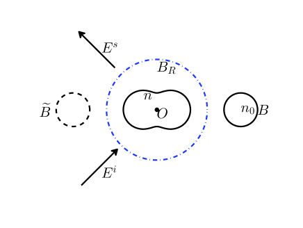
Figure 2: Scattering by an inhomogeneous medium.

Theorem 4.1.

Assume that $B$ is a given ball filled with the inhomogeneous medium of the refractive index $n_{0}\in C^{2,\gamma}({\mathbb{R}}^{3})$, $0<\gamma<1$, such that the support of $n_{0}-1$ is $\overline{B}$ and $k$ is not an electromagnetic interior transmission eigenvalue in $B$. Assume further that $n_{1},n_{2}\in C^{2,\gamma}({\mathbb{R}}^{3})$ are the refractive indices of two inhomogeneous media with $m_{j}:=n_{j}-1$ supported in $\overline{D_{j}}$, $j=1,2$. Suppose $\overline{D_{1}\cup D_{2}}\subset B_{R}$, where $B_{R}$ is a ball of radius $R$ and centered at the origin and satisfies that $\overline{B}\cap\overline{B_{R}}=\emptyset$. If the corresponding electric far-field patterns satisfy (3.4) for all $\hat{x}\in{\mathbb{S}}^{2}\setminus\{N,S\}$, $d_{1},d_{2}\in{\mathbb{S}}^{2}$, $m\in\{\phi,\theta\}$ and $p_{1},p_{2}\in{\mathbb{R}}^{3}$ satisfying that $d_{1}\bot p_{1}$ and $d_{2}\bot p_{2}$, then $n_{1}=n_{2}$.

To prove Theorem 4.1, we need the following lemma which is similar to Lemma 3.2.

Lemma 4.2.

Under the assumptions of Theorem 4.1, there does not hold the equation

$$E_{1}^{\infty}(\hat{x},d_{0})\bm{e}_{m}(d_{0})=e^{i\beta}\overline{E_{2}^{\infty}(\hat{x},d_{0})}\bm{e}_{m}(d_{0})\;\;\;\forall\hat{x}\in{\mathbb{S}}^{2},$$ (4.2)

where $m\in\{\phi,\theta\}$ and $d_{0}\in{\mathbb{S}}^{2}$ are arbitrarily fixed and $\beta$ is a real constant.

Proof.

Assume to the contrary that (4.2) holds. Then, by a similar argument as in the proof of Lemma 3.2 it can be derived that $E_{1}^{s}(\cdot,d_{0})\bm{e}_{m}(d_{0})$ and $H_{1}^{s}(\cdot,d_{0})\bm{e}_{m}(d_{0})$ can be analytically extended into ${\mathbb{R}}^{3}\setminus\overline{B_{R}}$ and satisfy the Maxwell equations (2.3a)–(2.3b) in ${\mathbb{R}}^{3}\setminus\overline{B_{R}}$. Noting that the incident waves $E^{i}(\cdot,d_{0})\bm{e}_{m}(d_{0})$ and $H^{i}(\cdot,d_{0})\bm{e}_{m}(d_{0})$ satisfy the Maxwell equations (2.3a)–(2.3b) in ${\mathbb{R}}^{3}$, we obtain that the total fields $E_{1}:=E_{1}(\cdot,d_{0})\bm{e}_{m}(d_{0})=E_{1}^{i}(\cdot,d_{0})\bm{e}_{m}(d_{0})+E_{1}^{s}(\cdot,d_{0})\bm{e}_{m}(d_{0})$ and $H_{1}:=(1/{ik}){\rm curl}\,E_{1}$ satisfy the Maxwell equations (2.3a)–(2.3b) in $B$.

On the other hand, from the definition of $\widetilde{n}_{1}$ and the electromagnetic medium scattering problem it follows that the total fields $E_{1}$ and $H_{1}$ also satisfy the first two Maxwell equations in (4.1) in $B$. Thus, $(\widetilde{E},\widetilde{H},E_{0},H_{0}):=(E_{1},H_{1},E_{1},H_{1})$ satisfies the problem (4.1). Since $k$ is not an electromagnetic interior transmission eigenvalue in $B$, it follows that $E_{1}\equiv 0$ in $B$. By the analyticity of the electric scattered field $E_{1}^{s}(\cdot,d_{0})\bm{e}_{m}(d_{0})$ in ${\mathbb{R}}^{3}\setminus\overline{B_{R}}$, it is easily seen that $E_{1}$ is also analytic in ${\mathbb{R}}^{3}\setminus\overline{B_{R}}$, and thus we have that $E_{1}\equiv 0$ in ${\mathbb{R}}^{3}\setminus\overline{B_{R}}$. This is a contradiction, implying that (4.2) dose not hold. The proof is then complete. ∎

With the aid of Lemma 4.2, we can now prove Theorem 4.1.

Proof of Theorem 4.1..

Our proof follows a similar argument as for the case of inverse obstacle scattering in Section 3. Arguing similarly as in the proof of Theorem 3.1, we can easily obtain (3.11). We now want to prove (3.12) for arbitrarily fixed $m\in\{\phi,\theta\}$. First, if $r(\hat{x},d,\bm{e}_{m}(\hat{x}),p)\equiv 0$ for $\hat{x}\in{\mathbb{S}}^{2}\setminus\{N,S\}$, $d\in{\mathbb{S}}^{2}$ and $p\in{\mathbb{R}}^{3}$, then it is obvious that (3.12) holds.

We now consider the case $r(\hat{x},d,\bm{e}_{m}(\hat{x}),p)\not\equiv 0$ for $\hat{x}\in{\mathbb{S}}^{2}\setminus\{N,S\}$, $d\in{\mathbb{S}}^{2}$ and $p\in{\mathbb{R}}^{3}$. By a similar argument as in the proof of Theorem 3.1 it can be shown that either (3.19) or (3.23) holds for some open set $U_{1}\subset{\mathbb{S}}^{2}\setminus\{N,S\}$, where $\alpha^{(m)}$ and $\beta^{(m)}$ are defined similarly as in (3.17) and (3.24), respectively, in the proof of Theorem 3.1. But, Lemma 4.2 implies that (3.23) does not hold. Thus we only need to consider the case when (3.19) holds. By (3.19) and Rellich’s lemma we obtain (3.20), where $G$ is defined as above. For any fixed $-d\in U_{1}$, define

$$\widetilde{E}:=[E^{i}(\cdot,d)+E^{s}_{1}(\cdot,d)]\bm{e}_{m}(d)-e^{i\alpha^{(m)}(-d)}[E^{i}(\cdot,d)+E^{s}_{2}(\cdot,d)]\bm{e}_{m}(d),\;\;\;\widetilde{H}:=(1/{ik}){\rm curl}\,\widetilde{E},$$

$$E_{0}:=\left(1-e^{i\alpha^{(m)}(-d)}\right)E^{i}(\cdot,d)\bm{e}_{m}(d),\;\;\;H_{0}:=(1/{ik}){\rm curl}\,E_{0}.$$

Then, by (3.20) we have $\widetilde{E}=E_{0}$ in $G$, and so $(\widetilde{E},\widetilde{H},E_{0},H_{0})$ satisfies the boundary conditions on $\partial B$ in the problem (4.1). Further, by the definition of $\widetilde{E}$, $\widetilde{H}$, $E_{0}$ and $H_{0}$ it is known that $(\widetilde{E},\widetilde{H},E_{0},H_{0})$ satisfies the problem (4.1). Since $k$ is not an electromagnetic interior transmission eigenvalue in $B$, we obtain that $e^{i\alpha^{(m)}(-d)}=1$ for all $-d\in U_{1}$, which means that (3.22) holds. By this and the analyticity of $E_{j}^{\infty}(\hat{x},d)\bm{e}_{m}(d)$ in $d\in{\mathbb{S}}^{2}\setminus\{N,S\}$, $j=1,2$, it follows that (3.12) is true. Similarly, we can show that (3.25) holds. Since $\overline{D_{1}\cup D_{2}}\subset B_{R}$ and $\overline{B}\cap\overline{B_{R}}=\emptyset$ then $\widetilde{n}_{j}\in C^{2,\gamma}({\mathbb{R}}^{3})$, $j=1,2$. Therefore, by (3.25) and [9, Theorem 4.9] we obtain that $n_{1}=n_{2}$. The proof is then complete. ∎

5 Conclusion

In this paper, by adding a given reference ball into the electromagnetic scattering system, we established uniqueness results for inverse electromagnetic obstacle and medium scattering with phaseless electric far-field data generated by infinitely many sets of superpositions of two electromagnetic plane waves with different directions and polarizations at a fixed frequency for the first time. These uniqueness results extend our previous results in [35] for the acoustic case to the electromagnetic case. Our method is based on a simple technique of using Rellich’s lemma and the Stratton–Chu formula for the radiating solutions to the Maxwell equations. In the future, we hope to show the same uniqueness results without using the reference ball, which is more challenging.

References

- [1] F. Cakoni, D. Colton and P. Monk, The electromagnetic inverse-scattering problem for partly coated Lipschitz domains, Proc. Roy. Soc. Edinburgh A 134 (2004), 661-682.
- [2] F. Cakoni, D. Colton and P. Monk, The Linear Sampling Method in Inverse Electromagnetic Scattering, SIAM, Philadelphia, PA, 2011.
- [3] X. Chen, Computational Methods for Electromagnetic Inverse Scattering, Wiley, 2018.
- [4] Z. Chen, S. Fang and G. Huang, A direct imaging method for the half-space inverse scattering problem with phaseless data, Inverse Probl. Imaging 11 (2017), 901-916.
- [5] Z. Chen and G. Huang, A direct imaging method for electromagnetic scattering data without phase information, SIAM J. Imaging Sci. 9 (2016), 1273-1297.
- [6] Z. Chen and G. Huang, Phaseless imaging by reverse time migration: Acoustic waves, Numer. Math., Theor. Meth. Appl. 10 (2017), 1-21.
- [7] D. Colton and R. Kress, The impedance boundary value problem for the time harmonic Maxwell equations, Math. Methods Appl. Sci. 3 (1981), 475-487.
- [8] D. Colton and R. Kress, Inverse Acoustic and Electromagnetic Scattering Theory (3rd Ed), Springer, New York, 2013.
- [9] P. Hähner, On Acoustic, Electromagnetic, and Elastic Scattering Problems in Inhomogeneous Media, Habilitation Thesis, University of Göttingen, 1998.
- [10] J. E. Hansen, Spherical Near-Field Antenna Measurements, The Institution of Engineering and Technology, London, 2008.
- [11] J. Li, H. Liu, and J. Zou, Strengthened linear sampling method with a reference ball, SIAM J. Sci. Comput. 31 (2009), 4013-4040.
- [12] O. Ivanyshyn, Shape reconstruction of acoustic obstacles from the modulus of the far field pattern, Inverse Probl. Imaging 1 (2007), 609-622.
- [13] O. Ivanyshyn and R. Kress, Identification of sound-soft 3D obstacles from phaseless data, Inverse Probl. Imaging 4 (2010), 131-149.
- [14] O. Ivanyshyn and R. Kress, Inverse scattering for surface impedance from phaseless far field data, J. Comput. Phys. 230 (2011), 3443-3452.
- [15] A. Kirsch and N. Grinberg, The factorization method for inverse problems, Oxford University Press, Oxford, 2008.
- [16] M.V. Klibanov, Phaseless inverse scattering problems in three dimensions, SIAM J. Appl. Math. 74 (2014), 392-410.
- [17] M.V. Klibanov, A phaseless inverse scattering problem for the 3-D Helmholtz equation, Inverse Probl. Imaging 11 (2017), 263-276.
- [18] M.V. Klibanov and V.G. Romanov, Reconstruction procedures for two inverse scattering problems without the phase information, SIAM J. Appl. Math. 76 (2016), 178-196.
- [19] M.V. Klibanov and V.G. Romanov, Uniqueness of a 3-D coefficient inverse scattering problem without the phase information, Inverse Problems 33 (2017) 095007.
- [20] R. Kress, Uniqueness in inverse obstacle scattering for electromagnetic waves, in: Proceedings of the URSI General Assembly, Maastricht, 2002.
- [21] R. Kress and W. Rundell, Inverse obstacle scattering with modulus of the far field pattern as data, in: Inverse Problems in Medical Imaging and Nondestructive Testing, Springer, Wien, 1997, pp. 75-92.
- [22] X. Liu and B. Zhang, Unique determination of a sound-soft ball by the modulus of a single far field datum, J. Math. Anal. Appl. 365 (2010), 619-624.
- [23] A. Majda, High frequency asymptotics for the scattering matrix and the inverse problem of acoustical scattering, Comm. Pure Appl. Math. 29 (1976), 261-291.
- [24] S. Maretzke and T. Hohage, Stability estimates for linearized near-field phase retrieval in X-ray phase contrast imaging, SIAM J. Appl. Math. 77 (2017), 384-408.
- [25] W. McLean, Strongly Elliptic Systems and Boundary Integral Equations, Cambridge Univ. Press, Cambridge, 2000.
- [26] R.G. Novikov, Formulas for phase recovering from phaseless scattering data at fixed frequency, Bull. Sci. Math. 139 (2015), 923-936.
- [27] R.G. Novikov, Explicit formulas and global uniqueness for phaseless inverse scattering in multidimensions, J. Geom. Anal. 26 (2016), 346-359.
- [28] L. Pan, Y. Zhong, X. Chen and S.P. Yeo, Subspace-based optimization method for inverse scattering problems utilizing phaseless data, IEEE Trans. Geosci. Remote Sensing 49 (2011), 981-987.
- [29] V.G. Romanov, The problem of recovering the permittivity coefficient from the modulus of the scattered electromagnetic field, Siberian Math. J. 58 (2017), 711-717.
- [30] V.G. Romanov and M. Yamamoto, Phaseless inverse problems with interference waves, J. Inverse Ill-posed Problems 26 (2018), 681-688.
- [31] C.H. Schmidt, S.F. Razavi, T.F. Eibert and Y. Rahmat-Samii, Phaseless spherical near-field antenna measurements for low and medium gain antennas, Adv. Radio Sci. 8 (2010), 43-48.
- [32] J. Shin, Inverse obstacle backscattering problems with phaseless data, Euro. J. Appl. Math. 27 (2016), 111-130.
- [33] F. Sun, D. Zhang and Y. Guo, Uniqueness in phaseless inverse scattering problems with superposition of incident point sources, arXiv:1812.03291v1, 2018.
- [34] X. Xu, B. Zhang and H. Zhang, Uniqueness in inverse scattering problems with phaseless far-field data at a fixed frequency, SIAM J. Appl. Math. 78 (2018), 1737-1753.
- [35] X. Xu, B. Zhang and H. Zhang, Uniqueness in inverse scattering problems with phaseless far-field data at a fixed frequency. II, SIAM J. Appl. Math. 78 (2018), 3024-3039.
- [36] X. Xu, B. Zhang and H. Zhang, Uniqueness and direct imaging method for inverse scattering by locally rough surfaces with phaseless near-field data, SIAM J. Imaging Sci. 12 (2019), 119-152.
- [37] X. Xu, B. Zhang and H. Zhang, Uniqueness in inverse acoustic and electromagnetic scattering with phaseless near-field data at a fixed frequency, arXiv:1906.05116, 2019.
- [38] B. Zhang and H. Zhang, Recovering scattering obstacles by multi-frequency phaseless far-field data, J. Comput. Phys. 345 (2017), 58-73.
- [39] B. Zhang and H. Zhang, Imaging of locally rough surfaces from intensity-only far-field or near-field data, Inverse Problems 33 (2017) 055001 (28pp).
- [40] B. Zhang and H. Zhang, Fast imaging of scattering obstacles from phaseless far-field measurements at a fixed frequency, Inverse Problems 34 (2018) 104005.
- [41] D. Zhang and Y. Guo, Uniqueness results on phaseless inverse scattering with a reference ball, Inverse Problems 34 (2018) 085002 (12pp).
- [42] D. Zhang, F. Sun, Y. Guo and H. Liu, Uniqueness in inverse acoustic scattering with phaseless near-field measurements, arXiv:1905.08242v1, 2019.
- [43] D. Zhang, Y. Wang, Y. Guo and J. Li, Uniqueness in inverse cavity scattering problems with phaseless near-field data, arXiv:1905.09819v1, 2019.
- [44] Y. Zhang and W. Wang, Robust array diagnosis against array mismatch using amplitude-only far field data, IEEE Access 7 (2019), 5589-5596.