Dynamics of stochastic gradient descent for two-layer neural networks in the teacher-student setup

Abstract

Deep neural networks achieve stellar generalisation even when they have enough parameters to easily fit all their training data. We study this phenomenon by analysing the dynamics and the performance of over-parameterised two-layer neural networks in the teacher-student setup, where one network, the student, is trained on data generated by another network, called the teacher. We show how the dynamics of stochastic gradient descent (SGD) is captured by a set of differential equations and prove that this description is asymptotically exact in the limit of large inputs. Using this framework, we calculate the final generalisation error of student networks that have more parameters than their teachers. We find that the final generalisation error of the student increases with network size when training only the first layer, but stays constant or even decreases with size when training both layers. We show that these different behaviours have their root in the different solutions SGD finds for different activation functions. Our results indicate that achieving good generalisation in neural networks goes beyond the properties of SGD alone and depends on the interplay of at least the algorithm, the model architecture, and the data set.

Deep neural networks behind state-of-the-art results in image classification and other domains have one thing in common: their size. In many applications, the free parameters of these models outnumber the samples in their training set by up to two orders of magnitude ^{1, 2}. Statistical learning theory suggests that such heavily over-parameterised networks generalise poorly without further regularisation ^{3, 4, 5, 6, 7, 8, 9}, yet empirical studies consistently find that increasing the size of networks to the point where they can easily fit their training data and beyond does not impede their ability to generalise well, even without any explicit regularisation ^{10, 11, 12}. Resolving this paradox is arguably one of the big challenges in the theory of deep learning.

One tentative explanation for the success of large networks has focused on the properties of stochastic gradient descent (SGD), the algorithm routinely used to train these networks. In particular, it has been proposed that SGD has an implicit regularisation mechanism that ensures that solutions found by SGD generalise well irrespective of the number of parameters involved, for models as diverse as (over-parameterised) neural networks ^{10, 13}, logistic regression ¹⁴ and matrix factorisation models ^{15, 16}.

In this paper, we analyse the dynamics of one-pass (or online) SGD in two-layer neural networks. We focus in particular on the influence of over-parameterisation on the final generalisation error. We use the teacher-student framework ^{17, 18}, where a training data set is generated by feeding random inputs through a two-layer neural network with $M$ hidden units called the teacher. Another neural network, the student, is then trained using SGD on that data set. The generalisation error is defined as the mean squared error between teacher and student outputs, averaged over all of input space. We will focus on student networks that have a larger number of hidden units $K\geq M$ than their teacher. This means that the student can express much more complex functions than the teacher function they have to learn; the students are thus over-parameterised with respect to the generative model of the training data in a way that is simple to quantify. We find this definition of over-parameterisation cleaner in our setting than the oft-used comparison of the number of parameters in the model with the number of samples in the training set, which is not well justified for non-linear functions. Furthermore, these two numbers surely cannot fully capture the complexity of the function learned in practical applications.

The teacher-student framework is also interesting in the wake of the need to understand the effectiveness of neural networks and the limitations of the classical approaches to generalisation ¹¹. Traditional approaches to learning and generalisation are data agnostic and seek worst-case type bounds ¹⁹. On the other hand, there has been a considerable body of theoretical work calculating the generalisation ability of neural networks for data arising from a probabilistic model, particularly within the framework of statistical mechanics ^{20, 21, 17, 22, 18}. Revisiting and extending the results that have emerged from this perspective is currently experiencing a surge of interest ^{23, 24, 25, 26, 27, 28}.

In this work we consider two-layer networks with a large input layer and a finite, but arbitrary, number of hidden neurons. Other limits of two-layer neural networks have received a lot of attention recently. A series of papers ^{29, 30, 31, 32} studied the mean-field limit of two-layer networks, where the number of neurons in the hidden layer is very large, and proved various general properties of SGD based on a description in terms of a limiting partial differential equation. Another set of works, operating in a different limit, have shown that infinitely wide over-parameterised neural networks trained with gradient-based methods effectively solve a kernel regression ^{33, 34, 35, 36, 37, 38}, without any feature learning. Both the mean-field and the kernel regime crucially rely on having an infinite number of nodes in the hidden layer, and the performance of the networks strongly depends on the detailed scaling used ^{38, 39}. Furthermore, a very wide hidden layer makes it hard to have a student that is larger than the teacher in a quantifiable way. This leads us to consider the opposite limit of large input dimension and finite number of hidden units.

Our main contributions are as follows:

(i) The dynamics of SGD (online) learning by two-layer neural networks in the teacher-student setup was studied in a series of classic papers ^{40, 41, 42, 43, 44} from the statistical physics community, leading to a heuristic derivation of a set of coupled ordinary differential equations (ODE) that describe the typical time-evolution of the generalisation error. We provide a rigorous foundation of the ODE approach to analysing the generalisation dynamics in the limit of large input size by proving their correctness.

(ii) These works focused on training only the first layer, mainly in the case where the teacher network has the same number of hidden units and the student network, $K=M$. We generalise their analysis to the case where the student’s expressivity is considerably larger than that of the teacher in order to investigate the over-parameterised regime $K>M$.

(iii) We provide a detailed analysis of the dynamics of learning and of the generalisation when only the first layer is trained. We derive a reduced set of coupled ODE that describes the generalisation dynamics for any $K\geq M$ and obtain analytical expressions for the asymptotic generalisation error of networks with linear and sigmoidal activation functions. Crucially, we find that with all other parameters equal, the final generalisation error increases with the size of the student network. In this case, SGD alone thus does not seem to be enough to regularise larger student networks.

(iv) We finally analyse the dynamics when learning both layers. We give an analytical expression for the final generalisation error of sigmoidal networks and find evidence that suggests that SGD finds solutions which amount to performing an effective model average, thus improving the generalisation error upon over-parameterisation. In linear and ReLU networks, we experimentally find that the generalisation error does change as a function of $K$ when training both layers. However, there exist student networks with better performance that are fixed points of the SGD dynamics, but are not reached when starting SGD from initial conditions with small, random weights.

Crucially, we find this range of different behaviours while keeping the training algorithm (SGD) the same, changing only the activation functions of the networks and the parts of the network that are trained. Our results clearly indicate that the implicit regularisation of neural networks in our setting goes beyond the properties of SGD alone. Instead, a full understanding of the generalisation properties of even very simple neural networks requires taking into account the interplay of at least the algorithm, the network architecture, and the data set used for training, setting up a formidable research programme for the future.

Reproducibility — We have packaged the implementation of our experiments and our ODE integrator into a user-friendly library with example programs at https://github.com/sgoldt/nn2pp. All plots were generated with these programs, and we give the necessary parameter values beneath each plot.

1 Online learning in teacher-student neural networks

We consider a supervised regression problem with training set $\mathcal{D}=\{(x^{\mu},y^{\mu})\}$ with $\mu=1,\ldots,P$. The components of the inputs $x^{\mu}\in\mathbb{R}^{N}$ are i.i.d. draws from the standard normal distribution $\mathcal{N}(0,1)$. The scalar labels $y^{\mu}$ are given by the output of a network with $M$ hidden units, a non-linear activation function $g:\mathbb{R}\to\mathbb{R}$ and fixed weights $\theta^{*}=(v^{*}\in\mathbb{R}^{M},w^{*}\in\mathbb{R}^{M\times N})$ with an additive output noise $\zeta^{\mu}\sim\mathcal{N}(0,1)$, called the teacher (see also Fig. 1a):

$$y^{\mu}\equiv\phi(x^{\mu},\theta^{*})+\sigma\zeta^{\mu},\qquad\textrm{where}\quad\phi(x,\theta^{*})=\sum_{m=1}^{M}v^{*}_{m}g\left(\frac{w^{*}_{m}x}{\sqrt{N}}\right)=\sum_{m}^{M}v^{*}_{m}g(\rho_{m})\,,$$ (1)

where $w^{*}_{m}$ is the $m$th row of $w^{*}$, and the local field of the $m$th teacher node is $\rho_{m}\equiv w^{*}_{m}x/\sqrt{N}$. We will analyse three different network types: sigmoidal with $g(x)=\operatorname{erf}(x/\sqrt{2})$, ReLU with $g(x)=\max(x,0)$, and linear networks where $g(x)=x$.

A second two-layer network with $K$ hidden units and weights $\theta=(v\in\mathbb{R}^{K},w\in\mathbb{R}^{K\times N})$, called the student, is then trained using SGD on the quadratic training loss $E(\theta)\propto\sum_{\mu=1}^{P}{\left[\phi(x^{\mu},\theta)-y^{\mu}\right]}^{2}$. We emphasise that the student network may have a larger number of hidden units $K\geq M$ than the teacher and thus be over-parameterised with respect to the generative model of its training data.

The SGD algorithm defines a Markov process $X^{\mu}\equiv\left[v^{*},w^{*},v^{\mu},w^{\mu}\right]$ with update rule given by the coupled SGD recursion relations

$$w_{k}^{\mu+1} =w_{k}^{\mu}-\frac{\eta_{w}}{\sqrt{N}}v_{k}^{\mu}g^{\prime}(\lambda_{k}^{\mu})\Delta^{\mu}x^{\mu},$$ (2)

$$v_{k}^{\mu+1} =v_{k}^{\mu}-\frac{\eta_{v}}{N}g(\lambda_{k}^{\mu})\Delta^{\mu}.$$ (3)

We can choose different learning rates $\eta_{v}$ and $\eta_{w}$ for the two layers and denote by $g^{\prime}(\lambda_{k}^{\mu})$ the derivative of the activation function evaluated at the local field of the student’s $k$th hidden unit $\lambda_{k}^{\mu}\equiv w_{k}x^{\mu}/\sqrt{N}$, and we defined the error term $\Delta^{\mu}\equiv\sum_{k}v_{k}^{\mu}g\left(\lambda_{k}^{\mu}\right)-\sum_{m}v^{*}_{m}g(\rho_{m}^{\mu})-\sigma\zeta^{\mu}$. We will use the indices $i,j,k,\ldots$ to refer to student nodes, and $n,m,\ldots$ to denote teacher nodes. We take initial weights at random from $\mathcal{N}(0,1)$ for sigmoidal networks, while initial weights have variance $1/\sqrt{N}$ for ReLU and linear networks.

The key quantity in our approach is the generalisation error of the student with respect to the teacher:

$$\epsilon_{g}(\theta,\theta^{*})\equiv\frac{1}{2}\left\langle{\left[\phi(x,\theta)-\phi(x,\theta^{*})\right]}^{2}\right\rangle,$$ (4)

where the angled brackets $\langle\cdot\rangle$ denote an average over the input distribution. We can make progress by realising that $\epsilon_{g}(\theta^{*},\theta)$ can be expressed as a function of a set of macroscopic variables, called order parameters in statistical physics,^{21, 40, 41}

$$Q^{\mu}_{ik}\equiv\frac{w^{\mu}_{i}w^{\mu}_{k}}{N},\quad R^{\mu}_{in}\equiv\frac{w^{\mu}_{i}w^{*}_{n}}{N}\quad\mathrm{and}\quad T_{nm}\equiv\frac{w^{*}_{n}w^{*}_{m}}{N},$$ (5)

together with the second-layer weights $v^{*}$ and $v^{\mu}$. Intuitively, the teacher-student overlaps $R^{\mu}=[R_{in}^{\mu}]$ measure the similarity between the weights of the $i$th student node and the $n$th teacher node. The matrix $Q_{ik}$ quantifies the overlap of the weights of different student nodes with each other, and the corresponding overlap of the teacher nodes are collected in the matrix $T_{nm}$. We will find it convenient to collect all order parameters in a single vector

$$m^{\mu}\equiv(R^{\mu},Q^{\mu},T,v^{*},v^{\mu}),$$ (6)

and we write the full expression for $\epsilon_{g}(m^{\mu})$ in Eq. (S31).

In a series of classic papers, Biehl, Schwarze, Saad, Solla and Riegler ^{40, 41, 42, 43, 44} derived a closed set of ordinary differential equations for the time evolution of the order parameters $m$ (see SM Sec. B). Together with the expression for the generalisation error $\epsilon_{g}(m^{\mu})$, these equations give a complete description of the generalisation dynamics of the student, which they analysed for the special case $K=M$ when only the first layer is trained ^{42, 44}. Our first contribution is to provide a rigorous foundation for these results under the following assumptions:

(A1)

Both the sequences $x^{\mu}$ and $\zeta^{\mu}$, $\mu=1,2,\ldots$, are i.i.d. random variables; $x^{\mu}$ is drawn from a normal distribution with mean 0 and covariance matrix $\mathbb{I}_{N}$, while $\zeta^{\mu}$ is a Gaussian random variable with mean zero and unity variance;

(A2)

The function $g(x)$ is bounded and its derivatives up to and including the second order exist and are bounded, too;

(A3)

The initial macroscopic state $m^{0}$ is deterministic and bounded by a constant;

(A4)

The constants $\sigma$, $K$, $M$, $\eta_{w}$ and $\eta_{v}$ are all finite.

The correctness of the ODE description is then established by the following theorem:

Theorem 1.1.

Choose $T\!>\!0$ and define $\alpha\equiv\mu/N$. Under assumptions (A1) – (A4), and for any $\alpha>0$, the macroscopic state $m^{\mu}$ satisfies

$$\max_{0\leq\mu\leq NT}\mathbb{E}\;\;||m^{\mu}-m(\alpha)||\leq\frac{C(T)}{\sqrt{N}}\,,$$ (7)

where $C(T)$ is a constant depending on $T$, but not on $N$, and $m(\alpha)$ is the unique solution of the ODE

$$\frac{\operatorname{d}\!}{\operatorname{d}\!t}m(\alpha)=f(m(\alpha))$$ (8)

with initial condition $m^{*}$. In particular, we have

$$\frac{\operatorname{d}\!R_{in}}{\operatorname{d}\!\alpha} \equiv f_{R}(m(\alpha)) =\eta v_{i}\langle\Delta g^{\prime}(\lambda_{i})\rho_{n}\rangle\,,$$ (9a)

$$\frac{\operatorname{d}\!Q_{ik}}{\operatorname{d}\!\alpha} \equiv f_{Q}(m(\alpha)) =\eta v_{i}\langle\Delta g^{\prime}(\lambda_{i})\lambda_{k}\rangle+\eta v_{k}\langle\Delta g^{\prime}(\lambda_{k})\lambda_{i}\rangle$$

$$\qquad+\eta^{2}v_{i}v_{k}\langle\Delta^{2}g^{\prime}(\lambda_{i})g^{\prime}(\lambda_{k})\rangle+\eta^{2}v_{i}v_{k}\sigma^{2}\langle g^{\prime}(\lambda_{i})g^{\prime}(\lambda_{k})\rangle\,,$$ (9b)

$$\frac{\operatorname{d}\!v_{i}}{\operatorname{d}\!\alpha} \equiv f_{v}(m(\alpha)) =\eta_{v}\langle\Delta g(\lambda_{i})\rangle.$$ (9c)

where all $f(m(\alpha))$ are uniformly Lipschitz continuous in $m(\alpha)$. We are able to close the equations because we can express averages in Eq. (9) in terms of only $m(\alpha)$.

We prove Theorem 1.1 using the theory of convergence of stochastic processes and a coupling trick introduced recently by Wang et al. ⁴⁵ in Sec. A of the SM. The content of the theorem is illustrated in Fig. 1b, where we plot $\epsilon_{g}(\alpha)$ obtained by numerically integrating (9) (solid) and from a single run of SGD (2) (crosses) for sigmoidal students and varying $K$, which are in very good agreement.

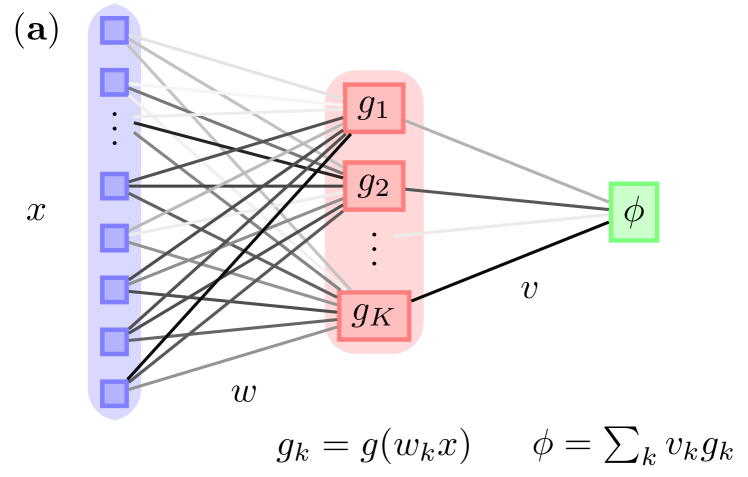
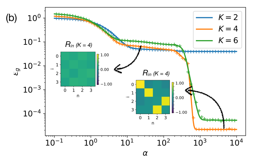
Figure 1: The analytical description of the generalisation dynamics of sigmoidal networks matches experiments. (a) We consider two-layer neural networks with a very large input layer. (b) We plot the learning dynamics $\epsilon_{g}(\alpha)$ obtained by integration of the ODEs (9) (solid) and from a single run of SGD (2) (crosses) for students with different numbers of hidden units $K$. The insets show the values of the teacher-student overlaps $R_{in}$ (5) for a student with $K=4$ at the two times indicated by the arrows. $N=784,M=4,\eta=0.2$.

Given a set of non-linear, coupled ODE such as Eqns. (9), finding the asymptotic fixed points analytically to compute the generalisation error would seem to be impossible. In the following, we will therefore focus on analysing the asymptotic fixed points found by numerically integrating the equations of motion. The form of these fixed points will reveal a drastically different dependence of the test error on the over-parameterisation of neural networks with different activation functions in the different setups we consider, despite them all being trained by SGD. This highlights the fact that good generalisation goes beyond the properties of just the algorithm. Second, knowledge of these fixed points allows us to make analytical and quantitative predictions for the asymptotic performance of the networks which agree well with experiments. We also note that several recent theorems ^{29, 31, 30} about the global convergence of SGD do not apply in our setting because we have a finite number of hidden units.

2 Asymptotic generalisation error of Soft Committee machines

We will first study networks where the second layer weights are fixed at $v^{*}_{m}=v_{k}=1$. These networks are called a Soft Committee Machine (SCM) in the statistical physics literature ^{40, 41, 42, 44, 18, 27}. One notable feature of $\epsilon_{g}(\alpha)$ in SCMs is the existence of a long plateau with sub-optimal generalisation error during training. During this period, all student nodes have roughly the same overlap with all the teacher nodes, $R_{in}=\mathrm{const.}$ (left inset in Fig. 1b). As training continues, the student nodes “specialise” and each of them becomes strongly correlated with a single teacher node (right inset), leading to a sharp decrease in $\epsilon_{g}$. This effect is well-known for both batch and online learning ¹⁸ and will be key for our analysis.

Let us now use the equations of motion (9) to analyse the asymptotic generalisation error of neural networks $\epsilon_{g}^{*}$ after training has converged and in particular its scaling with $L=K-M$. Our first contribution is to reduce the remaining $K(K+M)$ equations of motion to a set of eight coupled differential equations for any combination of $K$ and $M$ in Sec. C. This enables us to obtain a closed-form expression for $\epsilon_{g}^{*}$ as follows.

In the absence of output noise ($\sigma=0$), the generalisation error of a student with $K\geq M$ will asymptotically tend to zero as $\alpha\!\to\!\infty$. On the level of the order parameters, this corresponds to reaching a stable fixed point of (9) with $\epsilon_{g}=0$. In the presence of small output noise $\sigma>0$, this fixed point becomes unstable and the order parameters instead converge to another, nearby fixed point $m^{*}$ with $\epsilon_{g}(m^{*})>0$. The values of the order parameters at that fixed point can be obtained by perturbing Eqns. (9) to first order in $\sigma$, and the corresponding generalisation error $\epsilon_{g}(m^{*})$ turns out to be in excellent agreement with the generalisation error obtained when training a neural network using (2) from random initial conditions, which we show in Fig. 2a.

Sigmoidal networks.

We have performed this calculation for teacher and student networks with $g(x)=\operatorname{erf}(x/\sqrt{2})$. We relegate the details to Sec. C.2, and content us here to state the asymptotic value of the generalisation error to first order in $\sigma^{2}$,

$$\epsilon_{g}^{*}=\frac{\sigma^{2}\eta}{2\pi}f(M,L,\eta)+\mathcal{O}(\sigma^{3}),$$ (10)

where $f(M,L,\eta)$ is a lengthy rational function of its variables. We plot our result in Fig. 2a together with the final generalisation error obtained in a single run of SGD (2) for a neural network with initial weights drawn i.i.d. from $\mathcal{N}(0,1)$ and find excellent agreement, which we confirmed for a range of values for $\eta$, $\sigma$, and $L$.

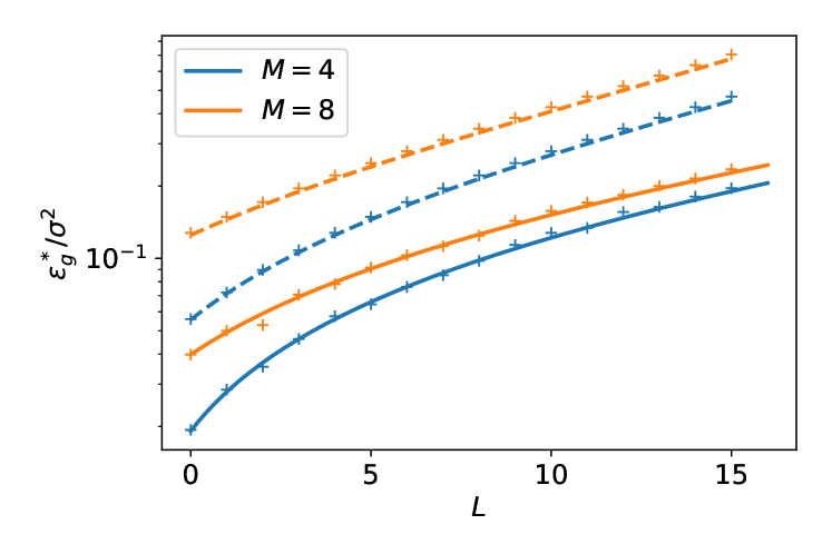
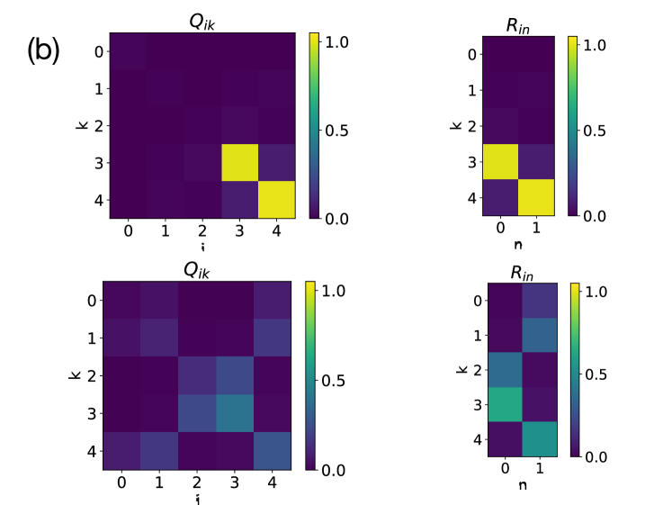
Figure 2: The asymptotic generalisation error of Soft Committee Machines increases with the network size. $N=784,\eta=0.05,\sigma=0.01$. (a) Our theoretical prediction for $\epsilon_{g}^{*}/\sigma^{2}$ for sigmoidal (solid) and linear (dashed), Eqns. (10) and (12), agree perfectly with the result obtained from a single run of SGD (2) starting from random initial weights (crosses). (b) The final overlap matrices $Q$ and $R$ (5) at the end of an experiment with $M=2,K=5$. Networks with sigmoidal activation function (top) show clear signs of specialisation as described in Sec. 2. ReLU networks (bottom) instead converge to solutions where all of the student’s nodes have finite overlap with teacher nodes.

One notable feature of Fig. 2a is that with all else being equal, SGD alone fails to regularise the student networks of increasing size in our setup, instead yielding students whose generalisation error increases linearly with $L$. One might be tempted to mitigate this effect by simultaneously decreasing the learning rate $\eta$ for larger students. However, lowering the learning rate incurs longer training times, which requires more data for online learning. This trade-off is also found in statistical learning theory, where models with more parameters (higher $L$) and thus a higher complexity class (e.g. VC dimension or Rademacher complexity ⁴) generalise just as well as smaller ones when given more data. In practice, however, more data might not be readily available, and we show in Fig. S2 of the SM that even when choosing $\eta=1/K$, the generalisation error still increases with $L$ before plateauing at a constant value.

We can gain some intuition for the scaling of $\epsilon_{g}^{*}$ by considering the asymptotic overlap matrices $Q$ and $R$ shown in the left half of Fig. 2b. In the over-parameterised case, $L=K-M$ student nodes are effectively trying to specialise to teacher nodes which do not exist, or equivalently, have weights zero. These $L$ student nodes do not carry any information about the teachers output, but they pick up fluctuations from output noise and thus increase $\epsilon_{g}^{*}$. This intuition is borne out by an expansion of $\epsilon_{g}^{*}$ in the limit of small learning rate $\eta$, which yields

$$\epsilon_{g}^{*}=\frac{\sigma^{2}\eta}{2\pi}\left(L+\frac{M}{\sqrt{3}}\right)+\mathcal{O}(\eta^{2}),$$ (11)

which is indeed the sum of the error of $M$ independent hidden units that are specialised to a single teacher hidden unit, and $L=K-M$ superfluous units contributing each the error of a hidden unit that is “learning” from a hidden unit with zero weights $w^{*}_{m}=0$ (see also Sec. D of the SM).

Linear networks.

Two possible explanations for the scaling $\epsilon_{g}^{*}\sim L$ in sigmoidal networks may be the specialisation of the hidden units or the fact that teacher and student network can implement functions of different range if $K\neq M$. To test these hypotheses, we calculated $\epsilon_{g}^{*}$ for linear neural networks ^{46, 47} with $g(x)=x$. Linear networks lack a specialisation transition ²⁷ and their output range is set by the magnitude of their weights, rather than their number of hidden units. Following the same steps as before, a perturbative calculation in the limit of small noise variance $\sigma^{2}$ yields

$$\epsilon_{g}^{*}=\frac{\eta\sigma^{2}(L+M)}{4-2\eta(L+M)}+\mathcal{O}(\sigma^{3}).$$ (12)

This result is again in perfect agreement with experiments, as we demonstrate in Fig. 2a. In the limit of small learning rates $\eta$, Eq. (10) simplifies to yield the same scaling as for sigmoidal networks,

$$\epsilon_{g}^{*}=\frac{1}{4}\eta\sigma^{2}(L+M)+\mathcal{O}\left(\eta^{2}\right).$$ (13)

This shows that the scaling $\epsilon_{g}^{*}\sim L$ is not just a consequence of either specialisation or the mismatched range of the networks’ output functions. The optimal number of hidden units for linear networks is $K=1$ for all $M$, because linear networks implement an effective linear transformation with an effective matrix $W=\sum_{k}w_{k}$. Adding hidden units to a linear network hence does not augment the class of functions it can implement, but it adds redundant parameters which pick up fluctuations from the teacher’s output noise, increasing $\epsilon_{g}$.

ReLU networks.

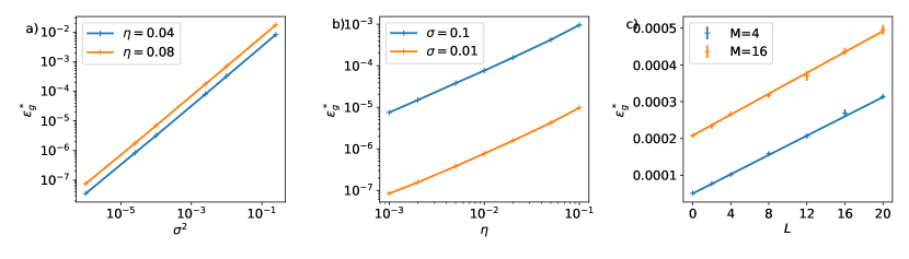
Figure S3: The final generalisation error of over-parametrised ReLU networks scales as $\epsilon_{g}^{*}\sim\eta\sigma^{2}L$. Simulations confirm that the asymptotic generalisation error $\epsilon_{g}^{*}$ of a ReLU student learning from a ReLU teacher scales with the learning rate $\eta$, the variance of the teacher’s output noise $\sigma^{2}$ and the number of additional hidden units as $\epsilon_{g}\sim\eta\sigma^{2}L$, which is the same scaling as the one found analytically for sigmoidal networks in Eq. (S49). Straight lines are linear fits to the data, with slope $1$ in (a) and (b). Parameters: $M=2,K=6$ (a, b) and $M=4,16$; $K=M+L$ (c); in all figures, $N=784,\kappa=0$.

The analytical calculation of $\epsilon^{*}_{g}$, described above, for ReLU networks poses some additional technical challenges, so we resort to experiments to investigate this case. We found that the asymptotic generalisation error of a ReLU student learning from a ReLU teacher has the same scaling as the one we found analytically for networks with sigmoidal and linear activation functions: $\epsilon_{g}^{*}\sim\eta\sigma^{2}L$ (see Fig. S3). Looking at the final overlap matrices $Q$ and $R$ for ReLU networks in the bottom half of Fig. 2b, we see that instead of the one-to-one specialisation of sigmoidal networks, all student nodes have a finite overlap with some teacher node. This is a consequence of the fact that it is much simpler to re-express the sum of $M$ ReLU units with $K\neq M$ ReLU units. However, there are still a lot of redundant degrees of freedom in the student, which all pick up fluctuations from the teacher’s output noise and increase $\epsilon_{g}^{*}$.

Discussion.

The key result of this section has been that the generalisation error of SCMs scales as

$$\epsilon_{g}^{*}\sim\eta\sigma^{2}L.$$ (14)

Before moving on the full two-layer network, we discuss a number of experiments that we performed to check the robustness of this result (Details can be found in Sec. G of the SM). A standard regularisation method is adding weight decay to the SGD updates (2). However, we did not find a scenario in our experiments where weight decay improved the performance of a student with $L>0$. We also made sure that our results persist when performing SGD with mini-batches. We investigated the impact of higher-order correlations in the inputs by replacing Gaussian inputs with MNIST images, with all other aspects of our setup the same, and the same $\epsilon_{g}$-$L$ curve as for Gaussian inputs. Finally, we analysed the impact of having a finite training set. The behaviour of linear networks and of non-linear networks with large but finite training sets did not change qualitatively. However, as we reduce the size of the training set, we found that the lowest asymptotic generalisation error was obtained with networks that have $K>M$.

3 Training both layers: Asymptotic generalisation error of a neural network

We now study the performance of two-layer neural networks when both layers are trained according to the SGD updates (2) and (3). We set all the teacher weights equal to a constant value, $v_{m}^{*}=v^{*}$, to ensure comparability between experiments. However, we train all $K$ second-layer weights of the student independently and do not rely on the fact that all second-layer teacher weights have the same value. Note that learning the second layer is not needed from the point of view of statistical learning: the networks from the previous section are already expressive enough to capture the students, and we are thus slightly increasing the over-parameterisation even further. Yet, we will see that the generalisation properties will be significantly enhanced.

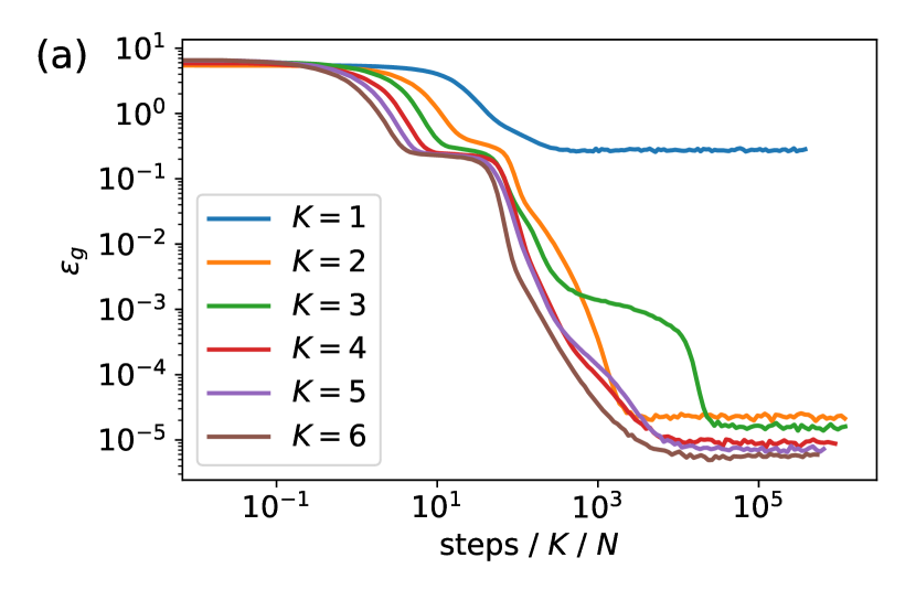
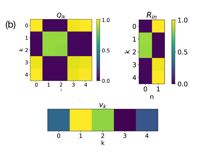
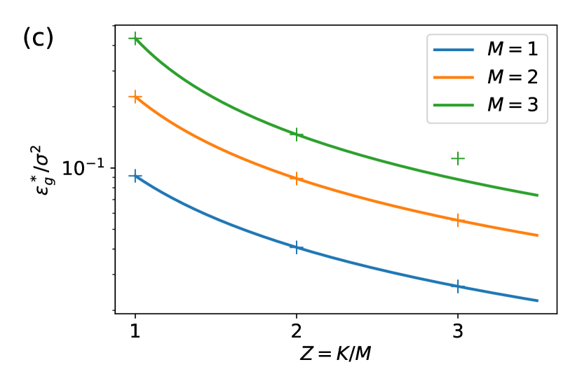
Figure 3: The performance of sigmoidal networks improves with network size when training both layers with SGD. (a) Generalisation dynamics observed experimentally for students with increasing $K$, with all other parameters being equal. ($N=500,M=2,\eta=0.05,\sigma=0.01,v^{*}=4$). (b) Overlap matrices $Q$, $R$, and second layer weights $v_{k}$ of the student at the end of the run with $K=5$ shown in (a). (c) Theoretical prediction for $\epsilon_{g}^{*}$ (solid) against $\epsilon_{g}^{*}$ observed after integration of the ODE until convergence (crosses) (9) ($\sigma=0.01,\eta=0.2,v^{*}=2$).

Sigmoidal networks.

We plot the generalisation dynamics of students with increasing $K$ trained on a teacher with $M=2$ in Fig. 3a. Our first observation is that increasing the student size $K\geq M$ decreases the asymptotic generalisation error $\epsilon_{g}^{*}$, with all other parameters being equal, in stark contrast to the SCMs of the previous section.

A look at the order parameters after convergence in the experiments from Fig. 3a reveals the intriguing pattern of specialisation of the student’s hidden units behind this behaviour, shown for $K=5$ in Fig. 3b. First, note that all the hidden units of the student have non-negligible weights ($Q_{ii}>0$). Two student nodes ($k=1,2$) have specialised to the first teacher node, i.e. their weights are very close to the weights of the first teacher node ($R_{10}\approx R_{20}\approx 0.85$). The corresponding second-layer weights approximately fulfil $v_{1}+v_{3}\approx v^{*}$. Summing the output of these two student hidden units is thus approximately equivalent to an empirical average of two estimates of the output of the teacher node. The remaining three student nodes all specialised to the second teacher node, and their outgoing weights approximately sum to $v^{*}$. This pattern suggests that SGD has found a set of weights for both layers where the student’s output is a weighted average of several estimates of the output of the teacher’s nodes. We call this the denoising solution and note that it resembles the solutions found in the mean-field limit of an infinite hidden layer ^{29, 31} where the neurons become redundant and follow a distribution dynamics (in our case, a simple one with few peaks, as e.g. Fig. 1 in ³¹).

We confirmed this intuition by using an ansatz for the order parameters that corresponds to a denoising solution to solve the equations of motion (9) perturbatively in the limit of small noise to calculate $\epsilon_{g}^{*}$ for sigmoidal networks after training both layers, similarly to the approach in Sec. 2. While this approach can be extended to any $K$ and $M$, we focused on the case where $K=ZM$ to obtain manageable expressions; see Sec. E of the SM for details on the derivation. While the final expression is again too long to be given here, we plot it with solid lines in Fig. 3c. The crosses in the same plot are the asymptotic generalisation error obtained by integration of the ODE (9) starting from random initial conditions, and show very good agreement.

While our result holds for any $M$, we note from Fig. 3c that the curves for different $M$ are qualitatively similar. We find a particular simple result for $M=1$ in the limit of small learning rates, where:

$$\epsilon_{g}^{*}=\frac{\eta(\sigma v^{*})^{2}}{2\sqrt{3}K\pi}+\mathcal{O}(\eta\sigma^{2})\,.$$ (15)

This result should be contrasted with the $\epsilon_{g}\sim K$ behaviour found for SCM.

Experimentally, we robustly observed that training both layers of the network yields better performance than training only the first layer with the second layer weights fixed to $v^{*}$. However, convergence to the denoising solution can be difficult for large students which might get stuck on a long plateau where their nodes are not evenly distributed among the teacher nodes. While it is easy to check that such a network has a higher value of $\epsilon_{g}$ than the denoising solution, the difference is small, and hence the driving force that pushes the student out of the corresponding plateaus is small, too. These observations demonstrate that in our setup, SGD does not always find the solution with the lowest generalisation error in finite time.

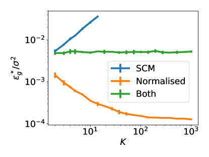
Figure 4: Asymptotic performance of linear two layer network. Error bars indicate one standard deviation over five runs. Parameters: $N=100,M=4,v^{*}=1,\eta=0.01,\sigma=0.01$.

ReLU and linear networks.

We found experimentally that $\epsilon_{g}^{*}$ remains constant with increasing $K$ in ReLU and in linear networks when training both layers. We plot a typical learning curve in green for linear networks in Fig. 4, but note that the figure shows qualitatively similar features for ReLU networks (Fig. S4). This behaviour was also observed in linear networks trained by batch gradient descent, starting from small initial weights ⁴⁸. While this scaling of $\epsilon_{g}^{*}$ with $K$ is an improvement over its increase with $K$ for the SCM, (blue curve), this is not the $1/K$ decay that we observed for sigmoidal networks. A possible explanation is the lack of specialisation in linear and ReLU networks (see Sec. 2), without which the denoising solution found in sigmoidal networks is not possible. We also considered normalised SCM, where we train only the first layer and fix the second-layer weights at $v^{*}_{m}=1/M$ and $v_{k}=1/K$. The asymptotic error of normalised SCM decreases with $K$ (orange curve in Fig. 4), because the second-layer weights $v_{k}=1/K$ effectively reduce the learning rate, as can be easily seen from the SGD updates (2), and we know from our analysis of linear SCM in Sec. 2 that $\epsilon_{g}\sim\eta$. In SM Sec. F we show analytically how imbalance in the norms of the first and second layer weights can lead to a larger effective learning rate. Normalised SCM also beat the performance students where we trained both layers, starting from small initial weights in both cases. This is surprising because we checked experimentally that the weights of a normalised SCM after training are a fixed point of the SGD dynamics when training both layers. However, we confirmed experimentally that SGD does not find this fixed point when starting with random initial weights.

Discussion.

The qualitative difference between training both or only the first layer of neural networks is particularly striking for linear networks, where fixing one layer does not change the class of functions the model can implement, but makes a dramatic difference for their asymptotic performance. This observation highlights two important points: first, the performance of a network is not just determined by the number of additional parameters, but also by how the additional parameters are arranged in the model. Second, the non-linear dynamics of SGD means that changing which weights are trainable can alter the training dynamics in unexpected ways. We saw this for two-layer linear networks, where SGD did not find the optimal fixed point, and in the non-linear sigmoidal networks, where training the second layer allowed the student to decrease its final error with every additional hidden unit instead of increasing it like in the SCM.

Dynamics of stochastic gradient descent for two-layer
neural networks in the teacher-student setup
SUPPLEMENTAL MATERIAL

Appendix A Proof of Theorem 1.1

A.1 Outline

We will prove Theorem 1.1 in two steps. First, we will show that the mean values of the order parameters $R_{in}$, $Q_{ik}$ and $v_{k}$ are given by the expressions used in the equations of motion (Lemma A.1) and that they concentrate, i.e. that their variance is bounded by a term of order $N^{-2}$. This ensures that the leading-order of the average increment is captured by the ODE of Theorem 1.1, and that the stochastic part of the increment of the order parameters can be ignored in the thermodynamic limit $N\to\infty$. In other words, the two bounds ensure that the stochastic Markov process converges to a deterministic process. To complete the proof, we use a form of the coupling trick as described by Wang et al. ⁴⁵.

A.2 First moments of the increment $m^{\mu}$

Throughout this paper, we use the convention that $\mathbb{E}\;$ indicates an average over all the random variables that follow, while $\mathbb{E}_{\mu}$ denotes the conditional expectation of all the random variables that follow conditioned on the state of the Markov chain at step $\mu$, $m^{\mu}$.

Lemma A.1.

Under the same setting as Theorem 1.1, for all $\mu<NT$, we have

$$\mathbb{E}\;|\mathbb{E}_{\mu}\;m^{\mu+1}-m^{\mu}-\frac{1}{N}f(m^{\mu})|\leq CN^{-3/2}.$$ (S1)

Proof.

We first recall that $m^{\mu}$ contains all time-dependent order parameters $R^{\mu}$, $Q^{\mu}$, and $v^{\mu}$, so we will prove the Lemma in turn for each of them. In fact, in each case we can prove a slightly stronger result which encompasses the required bound.

For the teacher-student overlaps $R_{in}^{\mu}$, we multiply the update (2) with $w^{*}_{n}/N$ on both sides and find that

$$R_{in}^{\mu+1}=R_{in}^{\mu}-\frac{\eta_{w}}{N}v_{i}\rho_{n}^{\mu}g^{\prime}(\lambda_{i}^{\mu})\Delta^{\mu}\,.$$ (S2)

The local field of the teacher is $\rho_{n}^{\mu}\equiv w^{*}_{n}x^{\mu}/\sqrt{N}$ is a Gaussian random variable with mean zero and variance $T_{nn}$. Taking the conditional expectation, we find

$$\mathbb{E}_{\mu}\;R_{in}^{\mu+1}-R_{in}^{\mu}=\frac{1}{N}\eta_{w}v_{i}\langle\rho_{n}^{\mu}\Delta^{\mu}g^{\prime}(\lambda_{i}^{\mu})\rangle$$ (S3)

as required.

For the student-student overlaps $Q_{ik}^{\mu}$, we multiply the update (2) by $w_{k}^{\mu}/N$ and find that

$$\begin{split}Q_{ik}^{\mu+1}&=Q_{ik}^{\mu}-\frac{1}{N}\left(\eta_{w}\Delta^{\mu}v^{\mu}_{k}g^{\prime}(\lambda_{k}^{\mu})\lambda_{i}^{\mu}+\eta_{w}\Delta^{\mu}v^{\mu}_{i}g^{\prime}(\lambda_{i}^{\mu})\lambda_{k}^{\mu}\right)\\ &\qquad+\frac{1}{N}\left(\eta_{w}^{2}{(\Delta^{\mu})}^{2}v_{i}^{\mu}v_{k}^{\mu}g^{\prime}(\lambda_{i}^{\mu})g^{\prime}(\lambda_{k}^{\mu})\frac{{(x^{\mu})}^{2}}{N}\right)\,.\end{split}$$ (S4)

Using assumption (A1), we see that the term ${(x^{\mu})}^{2}/N$ concentrates to yield 1 by the central limit theorem. Thus we find after taking the conditional expectation of both sides and using $\mathbb{E}_{\mu}\;\zeta^{\mu}=0$ that

$$\mathbb{E}_{\mu}\;Q_{ik}^{\mu+1}-Q_{ik}^{\mu}=\frac{1}{N}f_{Q}(m^{\mu})\,.$$ (S5)

Finally, it is easy to convince oneself that taking the conditional expectation of the update for the second-layer weights (3) yields

$$\mathbb{E}_{\mu}\;v_{k}^{\mu+1}-v_{k}^{\mu}=\frac{1}{N}f_{v}(m^{\mu})$$ (S6)

which completes the proof of Lemma A.1. ∎

A.3 Second moments of the increment $m^{\mu}$

We now proceed to bound the second-order moments of the increments of the time-dependent order parameters. We collect these bounds in the following lemma:

Lemma A.2.

Under the assumptions of Theorem 1.1, for all $\mu<NT$, we have that

$$\mathbb{E}\;{||m^{\mu+1}-\mathbb{E}_{\mu}\;m^{\mu+1}||}^{2}\leq C(T)N^{-2}\,.$$ (S7)

Before proceeding with the proof, we state a simple technical lemma that will be helpful in the following; we relegate its proof to Sec. A.5.

Lemma A.3.

Under the same assumptions as Theorem 1.1, we have for all $0\leq\mu\leq NT$ that

$$\mathbb{E}\;v_{k}^{\mu}\leq C(T)\,,$$ (S8)

where $C(T)$ is a constant independent of $N$.

In the following, we will use $q$ to denote any order-parameter that is varying in time, such as the teacher-student overlaps $R_{in}^{\mu}$, while we keep $m^{\mu}$ as the collection of all order parameters, including those that are static, such as the teacher-teacher overlaps $T_{nm}$.

Proof of Lemma A.2.

We first note all order parameters $q\in\left\{R_{in},Q_{ik},v_{k}\right\}$ obey update equations of the form

$$q^{\mu+1}=q^{\mu}+\frac{1}{N}f_{q}(m^{\mu},x^{\mu})\,,$$ (S9)

where we have emphasised that the update function $f_{q}(\cdot)$ may depend on all order parameters at time $\mu$ and the $\mu$th sample shown to the student $x^{\mu}$. For the variance $\sigma_{q}^{2}=\mathbb{E}\;(q-\mathbb{E}\;q)^{2}$ of the order parameter $q$, a little algebra yields the recursion relation

$$\begin{split}\left(\sigma_{q}^{\mu+1}\right)^{2}-\left(\sigma_{q}^{\mu}\right)^{2}&=\frac{2}{N}\left(\mathbb{E}\;q^{\mu}f_{q}(m^{\mu},x^{\mu})-\mathbb{E}\;f_{q}(m^{\mu},x^{\mu})\mathbb{E}\;q^{\mu}\right)\\ &\qquad+\frac{1}{N^{2}}\left(\mathbb{E}\;f_{q}(m^{\mu},x^{\mu})^{2}-\left[\mathbb{E}\;f_{q}(m^{\mu},x^{\mu})\right]^{2}\right).\end{split}$$ (S10)

We will now use complete induction to show that for any $q$, the update of the variance at every step is bounded by $C(T)N^{-2}$ as required. In particular, this means showing that the term proportional to $N^{-1}$ actually scales as $N^{-2}$.

For the induction start, we note that by Assumption A3, we have $\sigma_{q}^{0}=0$. Hence the variance of any order parameter after a single step of SGD reads

$$(\sigma_{q}^{1})^{2} =\frac{2}{N}\left(\mathbb{E}\;q^{0}\mathbb{E}\;f_{q}(m^{0},x^{0})-\mathbb{E}\;f_{q}(m^{0},x^{0})\mathbb{E}\;q^{0}\right)$$

$$\qquad+\frac{1}{N^{2}}\left(\mathbb{E}\;f_{q}(m^{0},x^{0})^{2}-\left[\mathbb{E}\;f_{q}(m^{0},x^{0})\right]^{2}\right)$$ (S11)

$$=\frac{1}{N^{2}}\left(\mathbb{E}\;f_{q}(m^{0},x^{0})^{2}-\left[\mathbb{E}\;f_{q}(m^{0},x^{0})\right]^{2}\right)\,.$$ (S12)

In going from the first to the second line, we have used assumption (A3) by which the initial macroscopic state is deterministic and therefore the average $\mathbb{E}\;$ is just an average over the first sample shown during training, which leads to the simplification of Eq. S12.

For the induction step, we assume that the variance after $\mu<T$ steps is $(\sigma^{\mu}_{v})^{2}\leq C(T)\mu N^{-2}\leq C(T)\alpha N^{-1}$. By using the existence and boundedness of the derivatives of the activation function, we can write $m^{\mu}=\mathbb{E}\;m^{\mu}+(m^{\mu}-\mathbb{E}\;m^{\mu})$ and expand the terms proportional to $N^{-1}$ using a multivariate Taylor expansion in $(m^{\mu}-\mathbb{E}\;m^{\mu})$. We find that

$$\left(\mathbb{E}\;q^{\mu}f_{q}(m^{\mu},x^{\mu})-\mathbb{E}\;f_{q}(m^{\mu},x^{\mu})\mathbb{E}\;q^{\mu}\right)\leq C(T)\mathbb{E}\;(m^{\mu}-\mathbb{E}\;m^{\mu})\leq C(T)\sigma_{q}^{2}\leq C(T)\sigma_{q}N^{-1}.$$ (S13)

We are justified in truncating the expansion since we assumed that $\sigma_{q}^{2}\leq C(T)N^{-1}$. If the functions $f_{q}(m,x)$ are bounded by a constant, this completes the induction and shows that the variance of the increment of the order parameters is bounded by $C(T)N^{-2}$, as required.

It is easy to check that all three functions $f_{v}$, $f_{R}$ and $f_{Q}$ fulfil this condition because of the boundedness of $g(x)$ and its derivatives (A2) and of Lemma A.3, which completes the proof of Lemma A.2. ∎

A.4 Putting it all together

Having proved both Lemmas A.1 and A.2, we can proceed to prove Theorem 1.1 by using the coupling trick in the form given by Wang et al. ⁴⁵ for another online learning problem, namely the training of generative adversarial networks. We paraphrase the coupling trick as given by Wang et al. in the following to make the proof self-contained and refer to the supplemental material of their paper for additional details.

Proof of Theorem 1.1.

We first define a stochastic process $b^{\mu}$ that is coupled with the Markov process $m^{\mu}$ as

$$b^{\mu+1}=b^{\mu}+\frac{1}{N}g(m^{\mu})+m^{\mu+1}-\mathbb{E}_{\mu}\;m^{\mu+1}\,.$$ (S14)

This process lives in the same space as $m^{\mu}$. Wang et al. ⁴⁵ showed that for such a process, when Lemma A.1 holds, we have that

$$\mathbb{E}\;||b^{\mu}-m^{\mu}||\leq C(T)N^{-1/2}$$ (S15)

for all $\mu\leq NT$. We then define a deterministic process

$$d^{\mu+1}=d^{\mu}+\frac{1}{N}g(d^{\mu}),$$ (S16)

which is a standard first-order finite difference approximation of the equations of motion (9), and also lives in the space as $m^{\mu}$. Invoking a standard Euler argument for first-order finite differences gives

$$\mathbb{E}\;||d^{\mu}-m(\mu/N)||\leq C(T)N^{-1}.$$ (S17)

Wang et al. ⁴⁵ further showed that for such a process, using Lemma A.2, we have

$$\mathbb{E}\;||b^{\mu}-d^{\mu}||\leq C(T)N^{-1}.$$ (S18)

Finally, combining Eqs. (S15), (S18) and (S17), we have

$$\mathbb{E}\;||m^{\mu}-m(\mu/N)||\leq C(T)N^{-1/2}$$ (S19)

which completes the proof. ∎

A.5 Additional proof details

Proof of Lemma A.3.

The increment of $v_{k}$ reads explicitly

$$v_{k}^{\mu+1}-v_{k}^{\mu}=\frac{\eta_{v}}{N}\left[\sum_{m}v^{*}_{m}g(\rho_{m}^{\mu})-\sum_{k}v_{k}^{\mu}g\left(\lambda_{k}^{\mu}\right)-\sigma\zeta^{\mu}\right]\,.$$ (S20)

To bound the value of $v_{k}^{\mu}$ after $\mu$ steps, we consider the three terms in the sum $v_{k}^{\mu}=\sum_{s=1}^{\mu}v_{k}^{\mu}$ each in turn. We first note that the sum of the output noise variables $\zeta^{\mu}$ is a simple sum over uncorrelated, (sub-) Gaussian random variables rescaled by $1/N$ and thus by Hoeffding’s inequality almost surely smaller than a constant ⁴⁹.

For the first two terms, we can use an argument similar to the one used to prove the bound on the variance of the increment of the order parameters. We first note that $g(\cdot)$ is a bounded function by Assumption (A2) and that the initial conditions of the second-layer weights are bounded by a constant by Assumption (A3). Hence, after a first step, the weight has increased by a term bounded by $C(T)N^{-1}$. Actually, at every step where the weight is bounded by a constant, its increase will be bounded by $C(T)N^{-1}$. Hence the magnitude of $v_{k}^{\mu}\leq C(T)$ for $0\leq\mu\leq NT$, as required. ∎

Appendix B Derivation of the ODE description of the generalisation dynamics of online learning

Here we demonstrate how to evaluate the averages found in the equations of motion for the order parameters (9), following the classic work by Biehl and Schwarze ⁴⁰ and Saad and Solla ^{41, 42}. We repeat the two main technical assumption of our work, namely having a large network ($N\to\infty$) and a data set that is large enough to allow that we visit every sample only once before training converges. Both will play a key role in the following computations.

B.1 Expressing the generalisation error in terms of order parameters

We first demonstrate how the assumptions stated above allow to rewrite the generalisation error in terms of a number of order parameters. We have

$$\epsilon_{g}(\theta,\theta^{*}) \equiv\frac{1}{2}\left\langle{\left[\phi(x,\theta)-\phi(x,\theta^{*})\right]}^{2}\right\rangle$$ (S21)

$$=\frac{1}{2}\left\langle{\left[\sum_{k=1}^{K}v_{k}g\left(\lambda_{k}\right)-\sum_{m=1}^{M}v^{*}_{m}g(\rho_{m})\right]}^{2}\right\rangle,$$ (S22)

where we have used the local fields $\lambda_{k}$ and $\rho_{m}$. Here and throughout this paper, we will use the indices $i,j,k,\ldots$ to refer to hidden units of the student, and indices $n,m,\ldots$ to denote hidden units of the teacher. Since the input $x^{\mu}$ only appears in $\epsilon_{g}$ only via products with the weights of the teacher and the student, we can replace the high-dimensional average $\langle\cdot\rangle$ over the input distribution $p(x)$ by an average over the $K+M$ local fields $\lambda_{k}^{\mu}$ and $\rho_{m}^{\mu}$. The assumption that the training set is large enough to allow that we visit every sample in the training set only once guarantees that the inputs and the weights of the networks are uncorrelated. Taking the limit $N\to\infty$ ensures that the local fields are jointly normally distributed with mean zero ($\langle x_{n}\rangle=0$). Their covariance is also easily found: writing $w_{ka}$ for the $a$th component of the $k$th weight vector, we have

$$\langle\lambda_{k}\lambda_{l}\rangle=\frac{\sum_{a,b}^{N}w_{ka}w_{lb}\langle x_{a}x_{b}\rangle}{N}=\frac{w_{k}w_{l}}{N}\equiv Q_{kl},$$ (S23)

since $\langle x_{a}x_{b}\rangle=\delta_{ab}$. Likewise, we define

$$\langle\rho_{n}\rho_{m}\rangle=\frac{w^{*}_{n}w^{*}_{m}}{N}\equiv T_{nm},\quad\langle\lambda_{k}\rho_{m}\rangle=\frac{w_{k}w^{*}_{m}}{N}\equiv R_{km}.$$ (S24)

The variables $R_{in}$, $Q_{ik}$, and $T_{nm}$ are called order parameters in statistical physics and measure the overlap between student and teacher weight vectors $w_{i}$ and $w^{*}_{n}$ and their self-overlaps, respectively. Crucially, from Eq. (S22) we see that they are sufficient to determine the generalisation error $\epsilon_{g}$. We can thus write the generalisation error as

$$\epsilon_{g}=\frac{1}{2}\sum_{i,k}v_{i}v_{k}I_{2}(i,k)+\frac{1}{2}\sum_{n,m}v^{*}_{n}v^{*}_{m}I_{2}(n,m)-\sum_{i,n}v_{i}v^{*}_{n}I_{2}(i,n),$$ (S25)

where we have defined

$$I_{2}(i,k)\equiv\langle g(\lambda_{i})g(\lambda_{k})\rangle.$$ (S26)

Assuming sigmoidal activation functions $g(x)=\operatorname{erf}(x/\sqrt{2})$ allows us to evaluate the average $I_{2}(i,k)$ analytically:

$$I_{2}(i,k)=\frac{1}{\pi}\arcsin\frac{Q_{ik}}{\sqrt{1+Q_{ii}}\sqrt{1+Q_{kk}}}.$$ (S27)

The average in Eq. (S26) is taken over a normal distribution for the local fields $\lambda_{i}$ and $\lambda_{k}$ with mean $(0,0)$ and covariance matrix

$$C_{2}=\begin{pmatrix}Q_{ii}&Q_{ik}\\ Q_{ik}&Q_{kk}\end{pmatrix}.$$ (S28)

Since we are using the indices $i,j,\ldots$ for student units and $n,m,\ldots$ for teacher hidden units, we have

$$I_{2}(i,n)=\langle g(\lambda_{i})g(\rho_{n})\rangle,$$ (S29)

where the covariance matrix of the joint of distribution $\lambda_{i}$ and $\rho_{m}$ is given by

$$C_{2}=\begin{pmatrix}Q_{ii}&R_{in}\\ T_{in}&T_{nn}\end{pmatrix}.$$ (S30)

and likewise for $I_{2}(n,m)$. We will use this convention to denote integrals throughout this section. For the generalisation error, this means that it can be expressed in terms of the order parameters alone as

$$\epsilon_{g}=\frac{1}{\pi}\sum_{i,k}v_{i}v_{k}\arcsin\frac{Q_{ik}}{\sqrt{1+Q_{ii}}\sqrt{1+Q_{kk}}}+\frac{1}{\pi}\sum_{n,m}v^{*}_{n}v^{*}_{m}\arcsin\frac{T_{nm}}{\sqrt{1+T_{nn}}\sqrt{1+T_{mm}}}\\ -\frac{2}{\pi}\sum_{i,n}v_{i}v^{*}_{n}\arcsin\frac{R_{in}}{\sqrt{1+Q_{ii}}\sqrt{1+T_{nn}}}.$$ (S31)

B.2 ODEs for the evolution of the order parameters

Expressing the generalisation error in terms of the order parameters as we have in Eq. (S31) is of course only useful if we can track the evolution of the order parameters over time. We can derive ODEs that allow us to do precisely that for the order parameters $Q$ by squaring the weight update of $w$ (2) and for $R$ taking the inner product of (2) with $w^{*}_{n}$, respectively, which yields the equations of motion (9).

To make progress however, i.e. to obtain a closed set of differential equations for $Q$ and $R$, we need to evaluate the averages $\langle\cdot\rangle$ over the local fields. In particular, we have to compute three types of averages:

$$I_{3}=\langle g^{\prime}(a)bg(c)\rangle,$$ (S32)

where $a$ is one the local fields of the student, while $b$ and $c$ can be local fields of either the student or the teacher;

$$I_{4}=\langle g^{\prime}(a)g^{\prime}(b)g(c)g(d)\rangle,$$ (S33)

where $a$ and $b$ are local fields of the student, while $c$ and $d$ can be local fields of both; and finally

$$J_{2}=\langle g^{\prime}(a)g^{\prime}(b)\rangle,$$ (S34)

where $a$ and $b$ are local fields of the teacher. In each of these integrals, the average is taken with respect to a multivariate normal distribution for the local fields with zero mean and a covariance matrix whose entries are chosen in the same way as discussed for $I_{2}$.

We can re-write Eqns. (9) with these definitions in a more explicit form as ^{41, 42, 43}

$$\frac{\operatorname{d}\!R_{in}}{\operatorname{d}\!t}=\eta v_{i}\left[\sum_{m}^{M}v^{*}_{m}I_{3}(i,n,m)-\sum_{j}^{K}v_{j}I_{3}(i,n,j)\right]\,,$$ (S35)

$$\begin{split}\frac{\operatorname{d}\!Q_{ik}}{\operatorname{d}\!t}&=\eta_{w}v_{i}\left[\sum_{m}^{M}v^{*}_{m}I_{3}(i,k,m)-\sum_{j}^{K}v_{j}I_{3}(i,k,j)\right]\\ &\quad+\eta_{w}v_{k}\left[\sum_{m}^{M}v^{*}_{m}I_{3}(k,i,m)-\sum_{j}^{K}v_{j}I_{3}(i,j,k)\right]\\ &\quad+\eta_{w}^{2}v_{i}v_{k}\left[\sum_{n}^{M}\sum_{m}^{M}v^{*}_{n}v^{*}_{m}I_{4}(i,k,n,m)-2\sum_{j}^{K}\sum_{n}^{M}v_{j}v^{*}_{n}I_{4}(i,k,j,n)\right.\\ &\qquad\qquad\qquad\left.+\sum_{j}^{K}\sum_{l}^{K}v_{j}v_{l}I_{4}(i,k,j,l)+\sigma^{2}J_{2}(i,k)\right]\end{split}$$ (S36)

$$\frac{\operatorname{d}\!v_{i}}{\operatorname{d}\!t}=\eta_{v}\left[\sum_{n}^{M}v^{*}_{n}I_{2}(i,n)-\sum_{j}^{K}v_{j}I_{2}(i,j)\right]\,.$$ (S37)

The explicit form of the integrals $I_{2}(\cdot)$, $I_{3}(\cdot)$, $I_{4}(\cdot)$ and $J_{2}(\cdot)$ is given in Sec. H for the case $g(x)=\operatorname{erf}\left(x/\sqrt{2}\right)$. Solving these equations numerically for $Q$ and $R$ and substituting their values in to the expression for the generalisation error (S25) gives the full generalisation dynamics of the student. We show the resulting learning curves together with the result of a single simulation in Fig. 2 of the main text. We have bundled our simulation software and our ODE integrator as a user-friendly library with example programs at https://github.com/sgoldt/nn2pp. In Sec. C, we discuss how to extract information from them in an analytical way.

Appendix C Calculation of $\epsilon_{g}$ in the limit of small noise for Soft Committee Machines

Our aim is to understand the asymptotic value of the generalisation error

$$\epsilon_{g}^{*}\equiv\lim_{\alpha\to\infty}\epsilon_{g}(\alpha).$$ (S38)

We focus on students that have more hidden units than the teacher, $K\geq M$. These students are thus over-parameterised with respect to the generative model of the data and we define

$$L\equiv K-M$$ (S39)

as the number of additional hidden units in the student network. In this section, we focus on the sigmoidal activation function

$$g(x)=\operatorname{erf}\left(x/\sqrt{2}\right),$$ (S40)

unless stated otherwise.

Eqns. (S35ff) are a useful tool to analyse the generalisation dynamics and they allowed Saad and Solla to gain plenty of analytical insight into the special case $K=M$ ^{41, 42}. However, they are also a bit unwieldy. In particular, the number of ODEs that we need to solve grows with $K$ and $M$ as $K^{2}+KM$. To gain some analytical insight, we make use of the symmetries in the problem, e.g. the permutation symmetry of the hidden units of the student, and re-parametrised the matrices $Q_{ik}$ and $R_{in}$ in terms of eight order parameters that obey a set of self-consistent ODEs for any $K>M$. We choose the following parameterisation with eight order parameters:

$$Q_{ij}= \begin{cases}Q&\quad i=j\leq M,\\ C&\quad i\neq j;\;i,j\leq M,\\ D&\quad i>M,j\leq M\quad\mathrm{or}\quad i\leq M,j>M,\\ E&\quad i=j>M,\\ F&\quad i\neq j;\;i,j>M,\end{cases}$$ (S41)

$$R_{in}= \begin{cases}R&\quad i=n,\\ S&\quad i\neq n;\;i\leq M,\\ U&\quad i>M,\end{cases}$$ (S42)

which in matrix form for the case $M=3$ and $K=5$ read:

$$R=\begin{pmatrix}R&S&S\\ S&R&S\\ S&S&R\\ U&U&U\\ U&U&U\end{pmatrix}\quad\mathrm{and}\quad Q=\begin{pmatrix}Q&C&C&D&D\\ C&Q&C&D&D\\ C&C&Q&D&D\\ D&D&D&E&F\\ D&D&D&F&E\\ \end{pmatrix}\,.$$ (S43)

We choose this number of order parameters and this particular setup for the overlap matrices $Q$ and $R$ for two reasons: it is the smallest number of variables for which we were able to self-consistently close the equations of motion (S35), and they agree with numerical evidence obtained from integrating the full equations of motion (S35).

By substituting this ansatz into the equations of motion (S35), we find a set of eight ODEs for the order parameters. These equations are rather unwieldy and some of them do not even fit on one page, which is why we do not print them here in full; instead, we provide a Mathematica notebook where they can be found and interacted with together with the source at http://www.github.com/sgoldt/nn2pp. These equations allow for a detailed analysis of the effect of over-parameterisation on the asymptotic performance of the student, as we will discuss now.

C.1 Heavily over-parameterised students can learn perfectly from a noiseless teacher using online learning

For a teacher with $T_{nm}=\delta_{nm}$ and in the absence of noise in the teacher’s outputs ($\sigma=0$), there exists a fixed point of the ODEs with $R=Q=1$, $C=D=E=F=0$, and perfect generalisation $\epsilon_{g}=0$. Online learning will find this fixed point ^{41, 42}. More precisely, after a plateau whose length depends on the size of the network for the sigmoidal network, the generalisation error eventually begins an exponential decay to the optimal solution with zero generalisation error. The learning rates are chosen such that learning converges, but aren’t optimised otherwise.

C.2 Perturbative solution of the ODEs

We have calculated the asymptotic value of the generalisation error $\epsilon_{g}^{*}$ for a teacher with $T_{nm}=\delta_{nm}$ to first order in the variance of the noise $\sigma^{2}$. To do so, we performed a perturbative expansion around the fixed point

$$R_{0}=Q_{0}=1,$$ (S44)

$$S_{0}=U_{0}=C_{0}=D_{0}=E_{0}=F_{0}=0,$$ (S45)

with the ansatz

$$X=X_{0}+\sigma^{2}X_{1}$$ (S46)

for all the order parameters. Writing the ODEs to first order in $\sigma^{2}$ and solving for their steady state where $X^{\prime}(\alpha)=0$ yielded a fixed point with an asymptotic generalisation error

$$\epsilon_{g}^{*}=\frac{\sigma^{2}\eta}{2\pi}f(M,L,\eta)+\mathcal{O}(\sigma^{3}).$$ (S47)

$f(M,L,\eta)$ is an unwieldy rational function of its variables. Due to its length, we do not print it here in full; instead, we give the full function in a Mathematica notebook together with our source code at https://github.com/anon/.... Here, we plot the results in various forms in Fig. S1. We note in particular the following points:

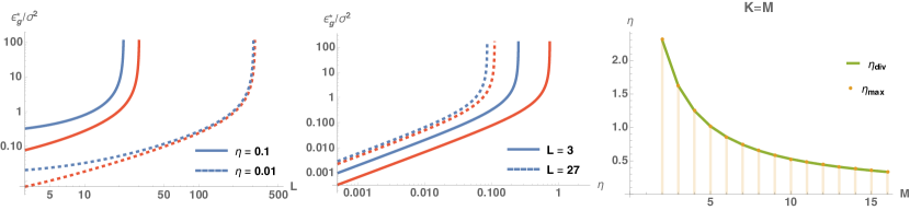
Figure S1: The final generalisation error of over-parameterised sigmoidal networks scales linearly with the learning rate, the variance of the teacher’s output noise, and $L$. We plot $\epsilon_{g}^{*}/\sigma^{2}$ in the limit of small noise, Eq. (S47), for $M=2$ (red) and $M=16$ (blue). It is clear that generalisation error increases with the number of superfluous units $L$ at fixed learning rate (left) and the learning rate $\eta$ (middle). Right: For $K=M$, the learning rate $\eta_{\mathrm{div}}$ at which our perturbative result diverges is precisely the maximum learning rate $\eta_{\max}$ at which the exponential convergence to the optimal solution is guaranteed for $\sigma=0$, Eq. (S48)

$\epsilon_{g}^{*}$ increases with $L$, $\eta$

The two plots on the left show that the generalisation error increases monotonically with both $L$ and $\eta$ while keeping the other fixed, respectively, for teachers with $M=2$ (red) and $M=16$ (blue)

The role of the learning rate $\eta$

Mitigating this effect by decreasing the learning rate $\eta$ for larger students raises two problems: a lower learning rate yields longer training times, and longer training times imply that more data is required until convergence. This is in agreement with statistical learning theory, where models with more parameters generalise just as well as smaller ones given enough data, despite having a higher complexity class as measured by VC dimension or Rademacher complexity ⁴, for example. Furthermore, we show in Sec. C.2 that even with $\eta\sim 1/K$, the generalisation error increases with $L$ before plateauing at a constant value. Moreover, we show in Fig. S2 that the asymptotic generalisation error (S47) of a student trained using SGD with learning rate $\eta=1/K$ still increases with $L$ before plateauing at a constant value that is independent of $M$.

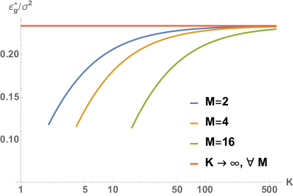
Figure S2: Asymptotic generalisation error for sigmoidal soft committee machines with learning rate $\eta=1/K$. We plot the asymptotic generalisation error $\epsilon_{g}^{*}$ (S47) over $\sigma^{2}$ of a student with a varying number of hidden units trained on data generated by teachers with $M=2,4,16$ using SGD with learning rate $1/K$. The generalisation error still increases with $K$, before plateauing at a constant value that is independent of $M$. Weight decay parameter $\kappa=0$.

Divergence at large $\eta$

Our perturbative result diverges for large $L$, or equivalently, for a large learning rate that depends on the number of hidden units $L\sim K$. For the special case $K=M$, the learning rate $\eta_{\mathrm{div}}$ at which our perturbative result diverges is precisely the maximum learning rate $\eta_{\max}$ for which the exponential convergence to the optimal solution is still guaranteed for $\sigma=0$ ⁴²

$$\eta_{\max}=\frac{\sqrt{3}\pi}{M+3/\sqrt{5}-1}$$ (S48)

as we show in the right-most plot of Fig. S1.

Expansion for small $\eta$

In the limit of small learning rates, which is the most relevant in practice and which from the plots in Fig. S1 dominates the behaviour of $\epsilon_{g}^{*}$ outside of the divergence, the generalisation error is linear in the learning rate. Expanding $\epsilon_{g}^{*}$ to first order in the learning rate reveals a particularly revealing form,

$$\epsilon_{g}^{*}=\frac{\sigma^{2}\eta}{2\pi}\left(L+\frac{M}{\sqrt{3}}\right)+\mathcal{O}(\eta^{2})$$ (S49)

with second-order corrections that are quadratic in $L$. This is actually the sum of the asymptotic generalisation errors of $M$ continuous perceptrons that are learning from a teacher with $T=1$ and $L$ continuous perceptrons with $T=0$ as we calculate in Sec. D. This neat result is a consequence of the specialisation that is typical of SCMs with sigmoidal activation functions as we discussed in the main text.

Appendix D Asymptotic generalisation error of a noisy continuous perceptron

What is the asymptotic generalisation for a continuous perceptron, i.e. a network with $K=1$, in a teacher-student scenario when the teacher has some additive Gaussian output noise? In this section, we repeat a calculation by Biehl and Schwarze ⁴⁰ where the teacher’s outputs are given by

$$y=g\left(\frac{w^{*}x}{\sqrt{N}}\right)+\zeta\,,$$ (S50)

where $\zeta$ is again a Gaussian r.v. with mean 0 and variance $\sigma^{2}$. We keep denoting the weights of the student by $w$ and the weights of the teacher by $w^{*}$. To analyse the generalisation dynamics, we introduce the order parameters

$$R\equiv\frac{ww^{*}}{N},\qquad Q\equiv\frac{ww}{N}\quad\mathrm{and}\quad T\equiv\frac{w^{*}w^{*}}{N}.$$ (S51)

and we explicitly do not fix $T$ for the moment. For $g(x)=\mathrm{erf}\left(x/\sqrt{2}\right)$, they obey the following equations of motion:

$$\frac{dR}{dt}= \frac{2\eta}{\pi\left(Q(t)+1\right)}\left(\frac{TQ(t)-{R(t)}^{2}+T}{\sqrt{(T+1)Q(t)-{R(t)}^{2}+T+1}}-\frac{R(t)}{\sqrt{2Q(t)+1}}\right)$$ (S52)

$$\frac{dQ}{dt}= \frac{4\eta}{\pi(Q(t)+1)}\left(\frac{R(t)}{\sqrt{2(Q(t)+1)-R(t)^{2}}}-\frac{Q(t)}{\sqrt{2Q(t)+1}}\right)$$

$$+\frac{4\eta^{2}}{\pi^{2}\sqrt{2Q(t)+1}}\left[-2\arcsin\left(\frac{R(t)}{\sqrt{(6Q(t)+2)(2Q(t)-R(t)^{2}+1)}}\right)\right.$$

$$\qquad+\left.\arcsin\left(\frac{2\left(Q(t)-R(t)^{2}\right)+1}{2\left(2Q(t)-R(t)^{2}+1\right)}\right)+\arcsin\left(\frac{Q(t)}{3Q(t)+1}\right)\right]$$

$$+\frac{2\eta^{2}\sigma^{2}}{\pi\sqrt{2Q(t)+1}}.$$ (S53)

The equations of motion have a fixed point at $Q=R=T$ which has perfect generalisation for $\sigma=0$. We hence make a perturbative ansatz in $\sigma^{2}$

$$Q(t)= T+\sigma^{2}q(t)$$ (S54)

$$R(t)= T+\sigma^{2}r(t)$$ (S55)

and find for the asymptotic generalisation error

$$\epsilon_{g}^{*}=\frac{\eta\sigma^{2}(4T+1)}{2\sqrt{2T+1}\left(-\eta\sqrt{8T^{2}+6T+1}+4\pi T+\pi\right)}+\mathcal{O}\left(\sigma^{3}\right).$$ (S56)

To first order in the learning rate, this reads

$$\epsilon_{g}^{*}=\frac{\eta\sigma^{2}}{2\pi\sqrt{2T+1}},$$ (S57)

which should be compared to the corresponding result for the full SCMs, Eq. (S49).

Appendix E Calculation of the asymptotic generalisation error in two-layer sigmoidal networks

In this section, we describe the ansatz we chose for the ODE to compute the asymptotic generalisation error when training both layers with sigmoidal activation function. As we describe in the main text, the ansatz used for the Soft Committee Machine is not appropriate, since (i) all the hidden units of the student are used, and (ii) several nodes overlap with the same teacher node. Inspection of the overlaps after integration of the ODE thus suggested the following ansatz when the number of nodes in the student is a multiple of the number of teacher nodes, $K=ZM$:

$$Q_{ij}= \begin{cases}Q&\quad i\mod M=j\mod M,\\ C&\quad\mathrm{otherwise}\end{cases}$$ (S58)

$$R_{in}= \begin{cases}R&\quad i\mod M=n\mod M,\\ S&\quad\mathrm{otherwise}\end{cases}$$ (S59)

which in matrix form for the case $M=2$ and $K=4$ read:

$$R_{in}=\begin{pmatrix}R&S\\ S&R\\ R&S\\ S&R\end{pmatrix}\quad\mathrm{and}\quad Q_{ik}=\begin{pmatrix}Q&C&Q&C\\ C&Q&C&Q\\ Q&C&Q&C\\ C&Q&C&Q\end{pmatrix}$$ (S60)

Once this ansatz is found, the rest of the calculation follows along the same lines as that of Sec. C: we derive a reduced set of coupled ODE for $Q,C,R$ and $S$, expand around the noiseless fixed point where $R=1,S=0,Q=1,C=0$ and substitute the resulting fixed point into the expression for the generalisation error, yielding the formula plotted in Fig. 3c.

In Fig. S4 we show the asymptotic performance linear and ReLU two-layer networks that we discuss at the end of Sec. 3 of the main text.

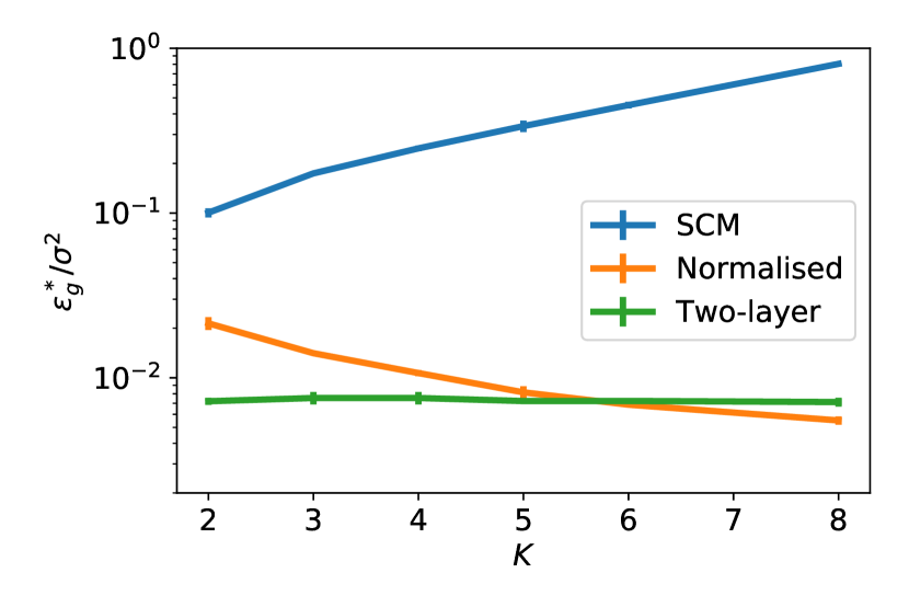
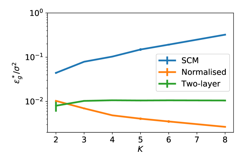
Figure S4: Asymptotic performance of linear (left) and ReLU (right) two layer networks. Error bars indicate one standard deviation over five runs, and the y-axis is the same in both plots. Parameters: $N=500,M=2,v^{*}=4,\eta=0.01,\sigma=0.01$. N.B. The right plot is the same as Fig. 4 of the main text.

Appendix F Unbalanced weights rescale effective learning rate in two layer linear networks

If we consider a linear, two layer neural network of the form:

$$\phi(x,\theta)=\sum_{m,j}{v_{m}w_{mj}x_{j}},$$ (S61)

where $v\in\mathbb{R}^{1\times M}$, $w\in\mathbb{R}^{M\times N}$ and $x\in\mathbb{R}^{N\times 1}$. The online SGD updates to the first and second layer weights will have the form:

$$\Delta w^{\mu}_{mj}=\eta(y^{\mu}-\phi(x^{\mu},\theta^{\mu}))v_{m}^{\mu}x_{j}^{\mu},$$ (S62)

and

$$\Delta v^{\mu}_{m}=\eta(y^{\mu}-\phi(x^{\mu},\theta^{\mu}))\sum_{j}{w_{mj}x_{j}^{\mu}}.$$ (S63)

If we define the product of student weights as a vector $u$:

$$u_{j}=\sum_{m=1}^{M}{v_{m}w_{mj}},$$ (S64)

it follows that

$$\Delta u_{j}^{\mu}=\sum_{m=1}^{M}{\left(v_{m}^{\mu}\Delta w^{\mu}_{mj}+\Delta v_{m}^{\mu}w^{\mu}_{mj}\right)}.$$ (S65)

Substituting the form for the update in first and second layer weights into the expression above we find:

$$\Delta u^{\mu}=\eta(y^{\mu}-u^{\mu}\cdot x^{\mu})(x^{\mu})^{T}\left(\mathbb{I}_{N}\|v^{\mu}\|^{2}+(w^{\mu})^{T}(w^{\mu})\right).$$ (S66)

This suggests that the level of imbalance between the norm of weights at different layers may impact the noisy fluctuations in updates even at late training times. If we compare the update step of the network with another network which produces the same output but has a different scaling of the weights we can see that the effective learning rate will be different. For instance $\tilde{v}=av$ and $\tilde{w}=\frac{1}{a}{w}$ leads to an equivalent network, but updates which scale as:

$$\Delta u^{\mu}=\eta(y^{\mu}-u^{\mu}\cdot x^{\mu})(x^{\mu})^{T}\left(\mathbb{I}_{N}a^{2}\|v^{\mu}\|^{2}+\frac{1}{a^{2}}(w^{\mu})^{T}(w^{\mu})\right).$$ (S67)

We can think of this scaling of the weights as impacting the effective learning, and we have provided an expression for how the learning rate impacts generalisation error in this paper. Our finding thus suggests that weights with more balanced norms across layers will tend to lead to lower generalisation error during online learning.

Appendix G Additional experiments on Soft Committee Machines

G.1 Regularisation by weight decay does not help

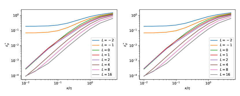
Figure S5: Weight decay. We plot the final generalisation error $\epsilon_{g}^{*}$ of a student with a varying number of hidden units trained on data generated by a teacher with $M=4$ using SGD with weight decay. The generalisation error clearly increases with the weight decay constant $\kappa$. Parameters: $N=784,\eta=0.1,\sigma=0.01$.

A natural strategy to avoid the pitfalls of overfitting is to regularise the weights, for example by using explicit weight decay by choosing $\kappa>0$. We have not found a setup where adding weight decay improved the asymptotic generalisation error of a student compared to a student that was trained without weight decay in our setup. As a consequence, weight decay completely fails to mitigate the increase of $\epsilon_{g}^{*}$ with $L$. We show the results of an illustrative experiment in Fig. S5.

G.2 SGD with mini-batches

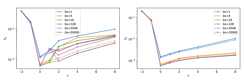
Figure S6: SGD with mini-batches shows the same qualitative behaviour as online learning We show the asymptotic generalisation error $\epsilon_{g}^{*}$ for students with sigmoidal (left) and ReLU activation function (right) for various $K$ learning from a teacher with $M=4$. Between the curves, we change the size of the mini-batch used at each step of SGD from $1$ (online learning) to 20 000. Parameters: $N=500,\eta=0.2,\sigma=0.1,\kappa=0$.

One key characteristic of online learning is that we evaluate the gradient of the loss function using a single sample from the training step per step. In practice, it is more common to actually use a number of samples $b>1$ to estimate the gradient at every step. To be more precise, the weight update equation for SGD with mini-batches would read:

$$w_{k}^{\mu+1}=w_{k}^{\mu}-\frac{\kappa}{N}w_{k}^{\mu}\\ -\frac{\eta}{b\sqrt{N}}\sum_{\ell=1}^{b}x^{\mu,\ell}g^{\prime}(\lambda_{k}^{\mu,\ell})\left[\phi(x^{\mu,\ell},\theta)-y^{\mu,\ell}\right].$$ (S68)

where $x^{\mu,\ell}$ is the $\ell$th input from the mini-batch used in the $m$th step of SGD, $\lambda_{k}^{\mu,\ell}$ is the local field of the $k$th student unit for the $\ell$th sample in the mini-batch, etc. Note that when we use every sample only once during training, using mini-batches of size $b$ increases the amount of data required by a factor $b$ when keeping the number of steps constant.

We show the asymptotic generalisation error of student networks of varying size trained using SGD with mini-batches and a teacher with $M=4$ in Fig. S6. Two trends are visible: first, using increasing the size of the mini-batches decreases the asymptotic generalisation error $\epsilon_{g}^{*}$ up to a certain mini-batch size, after which the gains in generalisation error become minimal; and second, the shape of the $\epsilon_{g}^{*}-L$ curve is the same for all mini-batch sizes, with the minimal generalisation error attained by a network with $K=M$.

G.3 Using MNIST images for training and testing

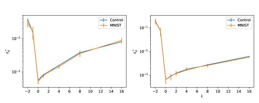
Figure S7: Higher-order correlations in the input data do not play a role for the asymptotic generalisation. We plot the final generalisation error $\epsilon_{g}^{*}$ after online learning of a student of various sizes from a teacher with $M=4$ using Gaussian inputs (blue) and MNIST images (red) for training and testing. $N=784,\eta=0.1,\sigma=0.1,\kappa=0$.

In the derivation of the ODE description of online learning for the main text, we noted that only the first two moments of the input distribution matter for the learning dynamics and for the final generalisation error. The reason for this is that the inputs only appear in the equations of motion for the order parameters as a product with the weights of either the teacher or the student. Now since they are – by assumption – uncorrelated with those weights, this product is the sum of large number of random variables and hence distributed by the central limit theorem.

We have checked how our results change when this assumption breaks down in one example where we train a network on a finite data set with non-trivial higher order moments, namely the images of the MNIST data set. We studied the very same setup that we discuss throughout this work, namely the supervised learning of a regression task in the teacher-student scenario. We only replace the the inputs, which would have been i.i.d. draws from the standard normal distribution, with the images of the MNIST data set. In particular, this means that we do not care about the labels of the images. Figure S7 shows a plot of the resulting final generalisation against $L$ for both the MNIST data set and a data set of the same size, comprised of i.i.d. draws from the standard normal distribution, which are in good agreement.

G.4 The scaling of $\epsilon^{*}_{g}$ with $L$ for finite training sets

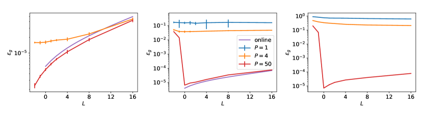
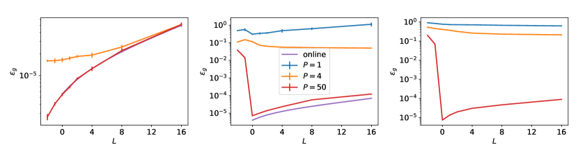
Figure S8: The scaling of $\epsilon_{g}^{*}$ with $L$ shows a similar dependence on the size of the training set for early-stopping (top) and final (bottom) generalisation error. We plot the asymptotic and the early-stopping generalisation error after SGD with a finite training set containing $PN$ samples (linear, sigmoidal and ReLU networks from left to right). The result for online learning for linear and sigmoidal networks, Eqns. (10) and (12) of the main text, are plotted in violet. Error bars indicate one standard deviation over 10 simulations, each with a different training set; many of them are too small to be clearly visible. Parameters: $N=784,M=4,\eta=0.1,\sigma=0.01$.

In practice, a single sample of the training data set will be visited several times during training. After a first pass through the training set, the online assumption that an incoming sample $(x,y)$ is uncorrelated to the weights of the network thus breaks down. A complete analytical treatment in this setting remains an open problem, so to study this practically relevant setup, we turn to simulations. We keep the setup described in Secs. 1, but simply reduce the number of samples in the training data set $P$. Our focus is again on the final generalisation error after convergence $\epsilon_{g}^{*}$ for linear, sigmoidal and ReLU networks, which we plot from left to right as a function of $L$ in Fig. S8.

Linear networks show a similar behaviour to the setup with a very large training set discussed in Sec. 2: the bigger the network, the worse the performance for both $P=4$ and $P=50$. Again, the optimal network has $K=1$ hidden units, irrespective of the size of the teacher. However, for non-linear networks, the picture is more varied: For large training sets, where the number of samples easily outnumber the free parameters in the network ($P=50$, red curve; this corresponds roughly to learning a data set of the size of MNIST), the behaviour is qualitatively described by our theory from Sec. 2: the best generalisation is obtained by a network that matches the teacher size, $K=M$. However, as we reduce the size of the training set, this is no longer true. For $P=4$, for example, the best generalisation is obtained with networks that have $K>M$. Thus the size of the training set with respect to the network has an important influence on the scaling of $\epsilon_{g}^{*}$ with $L$. Note that the early-stopping generalisation error, which we define as the minimal generalisation error over the duration of training, shows qualitatively the same behaviour as $\epsilon_{g}^{*}$.

G.5 Early-stopping generalisation error for finite training sets

A common way to prevent over-fitting of a neural network when training with a finite training set in practice is early stopping, where the training is stopped before the training error has converged to its final value yet. The idea behind early-stopping is thus to stop training before over-fitting sets in. For the purpose of our analysis of the generalisation of two-layer networks trained on a fixed finite data set in Sec. 4 of the main text, we define the early-stopping generalisation error $\hat{\epsilon}_{g}$ as the minimum of $\epsilon_{g}$ during the whole training process. In Fig. S8, we reproduce Fig. 6 from the main text at the bottom and plot $\hat{\epsilon}_{g}$ obtained from the very same experiments at the top. While the ReLU networks showed very little to no over-training, the sigmoidal networks showed more significant over-training. However, the qualitative dependence of the generalisation errors on $L$ was observed to be the same in this experiment. In particular, the early-stopping generalisation error also shows two different regimes, one where increasing the network hurts generalisation ($P\gg K$), and one where it improves generalisation or at least doesn’t seem to affect it much (small $P\sim K$).

Appendix H Explicit form of the integrals appearing in the equations of motion of sigmoidal networks

To be as self-contained as possible, here we collect the explicit forms of the integrals $I_{2}$, $I_{3}$, $I_{4}$ and $J_{2}$ that appear in the equations of motion for the order parameters and the generalisation error for networks with $g(x)=\operatorname{erf}\left(x/\sqrt{2}\right)$, see Eq. (S35). They were first given by ^{40, 41}. Each average $\langle\cdot\rangle$ is taken w.r.t. a multivariate normal distribution with mean 0 and covariance matrix $C\in\mathbb{R}^{n}$, whose components we denote with small letters. The integration variables $u,v$ are always components of $\lambda$, while $w$ and $z$ can be components of either $\lambda$ or $\rho$.

$$J_{2} \equiv\langle g^{\prime}(u)g^{\prime}(v)\rangle=\frac{2}{\pi}{\left(1+c_{11}+c_{22}+c_{11}c_{22}-c_{12}^{2}\right)}^{-1/2}$$ (S69)

$$I_{2} \equiv\frac{1}{2}\langle g(w)g(z)\rangle=\frac{1}{\pi}\arcsin\frac{c_{12}}{\sqrt{1+c_{11}}\sqrt{1+c_{12}}}.$$ (S70)

$$I_{3} \equiv\langle g^{\prime}(u)wg(z)\rangle=\frac{2}{\pi}\frac{1}{\sqrt{\Lambda_{3}}}\frac{c_{23}(1+c_{11})-c_{12}c_{13}}{1+c_{11}}$$ (S71)

$$I_{4} \equiv\langle g^{\prime}(u)g^{\prime}(v)g(w)g(z)\rangle=\frac{4}{\pi^{2}}\frac{1}{\sqrt{\Lambda_{4}}}\arcsin\left(\frac{\Lambda_{0}}{\sqrt{\Lambda_{1}\Lambda 2}}\right)$$ (S72)

where

$$\Lambda_{4}=(1+c_{11})(1+c_{22})-c_{12}^{2}$$ (S73)

and

$$\Lambda_{0} =\Lambda_{4}c_{34}-c_{23}c_{24}(1+c_{11})-c_{13}c_{14}(1+c_{22})+c_{12}c_{13}c_{24}+c_{12}c_{14}c_{23}$$ (S74)

$$\Lambda_{1} =\Lambda_{4}(1+c_{33})-c_{23}^{2}(1+c_{11})-c_{13}^{2}(1+c_{22})+2c_{12}c_{13}c_{23}$$ (S75)

$$\Lambda_{2} =\Lambda_{4}(1+c_{44})-c_{24}^{2}(1+c_{11})-c_{14}^{2}(1+c_{22})+2c_{12}c_{14}c_{24}$$ (S76)

References

- 1 Y. LeCun, Y. Bengio, and G.E. Hinton. Deep learning. Nature, 521(7553):436–444, 2015.
- 2 K. Simonyan and A. Zisserman. Very Deep Convolutional Networks for Large-Scale Image Recognition. In International Conference on Learning Representations, 2015.
- 3 P. L. Bartlett and S. Mendelson. Rademacher and Gaussian complexities: Risk bounds and structural results. Journal of Machine Learning Research, 3(3):463–482, 2003.
- 4 M. Mohri, A. Rostamizadeh, and A. Talwalkar. Foundations of Machine Learning. MIT Press, 2012.
- 5 B. Neyshabur, R. Tomioka, and N. Srebro. Norm-Based Capacity Control in Neural Networks. In Conference on Learning Theory, 2015.
- 6 N. Golowich, A. Rakhlin, and O. Shamir. Size-independent sample complexity of neural networks. Information and Inference: A Journal of the IMA, 2019.
- 7 G.K. Dziugaite and D.M. Roy. Computing Nonvacuous Generalization Bounds for Deep (Stochastic) Neural Networks with Many More Parameters than Training Data. In Proceedings of the Thirty-Third Conference on Uncertainty in Artificial Intelligence, 2017.
- 8 S. Arora, R. Ge, B. Neyshabur, and Y. Zhang. Stronger generalization bounds for deep nets via a compression approach. In 35th International Conference on Machine Learning, ICML 2018, pages 390–418, 2018.
- 9 Z. Allen-Zhu, Y. Li, and Y. Liang. Learning and Generalization in Overparameterized Neural Networks, Going Beyond Two Layers. arXiv:1811.04918, 2018.
- 10 B. Neyshabur, R. Tomioka, and N. Srebro. In search of the real inductive bias: On the role of implicit regularization in deep learning. In ICLR, 2015.
- 11 C. Zhang, S. Bengio, M. Hardt, B. Recht, and O. Vinyals. Understanding deep learning requires rethinking generalization. In ICLR, 2017.
- 12 D. Arpit, S. Jastrz, M.S. Kanwal, T. Maharaj, A. Fischer, A. Courville, and Y. Bengio. A Closer Look at Memorization in Deep Networks. In Proceedings of the 34th International Conference on Machine Learning, 2017.
- 13 P. Chaudhari and S. Soatto. On the inductive bias of stochastic gradient descent. In International Conference on Learning Representations, 2018.
- 14 D. Soudry, E. Hoffer, and N. Srebro. The implicit bias of gradient descent on separable data. In International Conference on Learning Representations, 2018.
- 15 S. Gunasekar, B. Woodworth, S. Bhojanapalli, B. Neyshabur, and N. Srebro. Implicit Regularization in Matrix Factorization. In Advances in Neural Information Processing Systems 30, pages 6151–6159, 2017.
- 16 Y. Li, T. Ma, and H. Zhang. Algorithmic Regularization in Over-parameterized Matrix Sensing and Neural Networks with Quadratic Activations. In Conference on Learning Theory, pages 2–47, 2018.
- 17 H. S. Seung, H. Sompolinsky, and N. Tishby. Statistical mechanics of learning from examples. Physical Review A, 45(8):6056–6091, 1992.
- 18 A. Engel and C. Van den Broeck. Statistical Mechanics of Learning. Cambridge University Press, 2001.
- 19 V. Vapnik. Statistical learning theory. New York, pages 156–160, 1998.
- 20 E. Gardner and B. Derrida. Three unfinished works on the optimal storage capacity of networks. Journal of Physics A: Mathematical and General, 22(12):1983–1994, 1989.
- 21 W. Kinzel, P. Ruján, and P. Rujan. Improving a Network Generalization Ability by Selecting Examples. EPL (Europhysics Letters), 13(5):473–477, 1990.
- 22 T.L.H. Watkin, A. Rau, and M. Biehl. The statistical mechanics of learning a rule. Reviews of Modern Physics, 65(2):499–556, 1993.
- 23 L. Zdeborová and F. Krzakala. Statistical physics of inference: thresholds and algorithms. Adv. Phys., 65(5):453–552, 2016.
- 24 M.S. Advani and S. Ganguli. Statistical mechanics of optimal convex inference in high dimensions. Physical Review X, 6(3):1–16, 2016.
- 25 P. Chaudhari, A. Choromanska, S. Soatto, Y. LeCun, C. Baldassi, C. Borgs, J. Chayes, L. Sagun, and R. Zecchina. Entropy-SGD: Biasing Gradient Descent Into Wide Valleys. In ICLR, 2017.
- 26 M.S. Advani and A.M. Saxe. High-dimensional dynamics of generalization error in neural networks. arXiv:1710.03667, 2017.
- 27 B. Aubin, A. Maillard, J. Barbier, F. Krzakala, N. Macris, and L. Zdeborová. The committee machine: Computational to statistical gaps in learning a two-layers neural network. In Advances in Neural Information Processing Systems 31, pages 3227–3238, 2018.
- 28 M. Baity-Jesi, L. Sagun, M. Geiger, S. Spigler, G.B. Arous, C. Cammarota, Y. LeCun, M. Wyart, and G. Biroli. Comparing Dynamics: Deep Neural Networks versus Glassy Systems. In Proceedings of the 35th International Conference on Machine Learning, 2018.
- 29 S. Mei, A. Montanari, and P. Nguyen. A mean field view of the landscape of two-layer neural networks. Proceedings of the National Academy of Sciences, 115(33):E7665–E7671, 2018.
- 30 G.M. Rotskoff and E. Vanden-Eijnden. Parameters as interacting particles: long time convergence and asymptotic error scaling of neural networks. In Advances in Neural Information Processing Systems 31, pages 7146–7155, 2018.
- 31 L. Chizat and F. Bach. On the global convergence of gradient descent for over-parameterized models using optimal transport. In Advances in Neural Information Processing Systems 31, pages 3040–3050, 2018.
- 32 J. Sirignano and K. Spiliopoulos. Mean field analysis of neural networks: A central limit theorem. Stochastic Processes and their Applications, 2019.
- 33 A. Jacot, F. Gabriel, and C. Hongler. Neural tangent kernel: Convergence and generalization in neural networks. In Advances in Neural Information Processing Systems 32, pages 8571–8580, 2018.
- 34 S.S. Du, X. Zhai, B. Poczos, and A. Singh. Gradient descent provably optimizes over-parameterized neural networks. In International Conference on Learning Representations, 2019.
- 35 Z. Allen-Zhu, Y. Li, and Z. Song. A convergence theory for deep learning via over-parameterization. arXiv preprint arXiv:1811.03962, 2018.
- 36 Y. Li and Y. Liang. Learning Overparameterized Neural Networks via Stochastic Gradient Descent on Structured Data. In Advances in Neural Information Processing Systems 31, 2018.
- 37 D. Zou, Y. Cao, D. Zhou, and Q. Gu. Stochastic gradient descent optimizes over-parameterized deep relu networks. Machine Learning, pages 1–26, 2019.
- 38 L. Chizat, E. Oyallon, and F. Bach. On lazy training in differentiable programming. In Advances in Neural Information Processing Systems 33, 2019.
- 39 S. Mei, T. Misiakiewicz, and A. Montanari. Mean-field theory of two-layers neural networks: dimension-free bounds and kernel limit. arXiv preprint arXiv:1902.06015, 2019.
- 40 M. Biehl and H. Schwarze. Learning by on-line gradient descent. J. Phys. A. Math. Gen., 28(3):643–656, 1995.
- 41 D. Saad and S.A. Solla. Exact Solution for On-Line Learning in Multilayer Neural Networks. Phys. Rev. Lett., 74(21):4337–4340, 1995.
- 42 D. Saad and S.A. Solla. On-line learning in soft committee machines. Phys. Rev. E, 52(4):4225–4243, 1995.
- 43 P. Riegler and M. Biehl. On-line backpropagation in two-layered neural networks. Journal of Physics A: Mathematical and General, 28(20), 1995.
- 44 D. Saad and S.A. Solla. Learning with Noise and Regularizers Multilayer Neural Networks. In Advances in Neural Information Processing Systems 9, pages 260–266, 1997.
- 45 C. Wang, Hong Hu, and Yue M. Lu. A Solvable High-Dimensional Model of GAN. arXiv:1805.08349, 2018.
- 46 A. Krogh and J. A. Hertz. Generalization in a linear perceptron in the presence of noise. Journal of Physics A: Mathematical and General, 25(5):1135–1147, 1992.
- 47 A.M. Saxe, James L. McClelland, and S. Ganguli. Exact solutions to the nonlinear dynamics of learning in deep linear neural networks. In ICLR, 2014.
- 48 A.K. Lampinen and S. Ganguli. An analytic theory of generalization dynamics and transfer learning in deep linear networks. In International Conference on Learning Representations, 2019.
- 49 R. Vershynin. High-Dimensional Probability. Cambridge University Press, 2009.