Energy Models for Better Pseudo-Labels: Improving Semi-Supervised Classification with the 1-Laplacian Graph Energy

Abstract

Semi-supervised classification is a great focus of interest, as in real-world scenarios obtaining labels is expensive, time-consuming and might require expert knowledge. This has motivated the fast development of semi-supervised techniques, whose performance is on a par with or better than supervised approaches. A current major challenge for semi-supervised techniques is how to better handle the network calibration and confirmation bias problems for improving performance. In this work, we argue that energy models are an effective alternative to such problems. With this motivation in mind, we propose a hybrid framework for semi-supervised classification called CREPE model (1-LaplaCian gRaph Energy for Pseudo-labEls). Firstly, we introduce a new energy model based on the non-smooth $\ell_{1}$ norm of the normalised graph 1-Laplacian. Our functional enforces a sufficiently smooth solution and strengthens the intrinsic relation between the labelled and unlabelled data. Secondly, we provide a theoretical analysis for our proposed scheme and show that the solution trajectory does converge to a non-constant steady point. Thirdly, we derive the connection of our energy model for pseudo-labelling. We show that our energy model produces more meaningful pseudo-labels than the ones generated directly by a deep network. We extensively evaluate our framework, through numerical and visual experiments, using six benchmarking datasets for natural and medical images. We demonstrate that our technique reports state-of-the-art results for semi-supervised classification.

1 Introduction

In this era of big data, deep learning (DL) has reported astonishing results for different tasks in computer vision. For the task of image classification, a major breakthrough has been reported in the setting of supervised learning. In this context, the majority of methods are based on deep convolutional neural networks e.g. [1, 2], in which pre-trained, fine-tuned and trained from scratch solutions have been considered. A key factor for these impressive results is the assumption of a large and well-representative corpus of labelled data. These labels can be generated either by humans or automatically on proxy tasks. However, obtaining well-annotated labels is expensive, time consuming and one should account for the inherent human bias and uncertainty that adversely effect the classification output. These drawbacks have motivated semi-supervised learning (SSL) [3, 4] to be a great focus of interest for the community.

The key idea of SSL is to leverage on a tiny labelled set and a large unlabelled set to produce a good classification output. The desirable advantages of this setting is that one can decrease the dependency on a large amount of well-annotated data whilst gaining further understanding of intrinsic data structures [3]. The body of literature has reported promising results, from the classic perspective, for semi-supervised classification using both transductive (e.g [5, 6, 7, 8, 9, 10, 11]) and inductive (e.g. [12, 13, 14]) philosophies. Those techniques seek to infer the labels for the large unlabelled set, relying solely on the tiny labelled set as prior, by minimising a given energy (i.e., energy models [3, 5, 6]). More recently, deep learning has also been applied in the SSL context - examples are [15, 16, 17, 18], where strong augmentations and costly optimisation schemes are key for the outstanding performance. Both perspectives have shown potentials but they still have limitations. Whilst energy models rely on hand-crafted features that are difficult to generalise, deep learning techniques lack of a well-defined theory.

A few recent works [19, 20, 21] have attempted to combine both perspectives, so-called hybrid models, where the principles of energy models and deep learning are combined. Hybrid models have demonstrated performance which readily competes against deep learning techniques [21]. However, similarly to deep learning techniques, hybrid models have been investigated mainly from the practical point of view. That is, in the context of hybrid models not much effort has been spent on developing better energy functionals and analysing their theoretical properties. This is the motivation that drives the basis for this work.

More precisely, in this work we propose a robust graph energy for semi-supervised classification following a hybrid setting. We focus on the normalised Dirichlet energy (2) based on the graph Laplacian. Promising results have already been shown in this context. For example, the seminal algorithmic approach of [6] was introduced to perform a graph transduction, through the propagation of few labels, by minimising the Laplacian graph energy (2) for the specific case when $p=2$. Subsequent machine learning studies showed that using non-smooth energies with the $p=1$ norm, related to non-local total variation, can achieve better clustering performances [22], but original algorithms only approximated $p\to 1$. More advanced optimisation tools were therefore proposed to consider the exact $p=1$ norm for binary [23] or multi-class [24] graph transduction. The normalisation of the operator is nevertheless crucial, as underlined in [25], to ensure within-cluster similarity when the degrees $d_{i}$ of the nodes are broadly distributed in the graph. These motivations drive our approach using the normalised Dirichlet energy (2) based on the graph Laplacian.

Contributions. Our work is motivated by the problems of network calibration and the confirmation bias in pseudo-labelling [26, 27, 28, 29], where one seeks that the probability of the predicted label reflects the ground truth correctness likelihood. In particular, in the context of deep learning a current major family of techniques is pseudo-labelling. In this perspective, a current challenge is how to improve poorly calibrated networks for better pseudo-labels [28, 30]. In this work, we argue that energy models can be a powerful alternative for inferring more meaningful pseudo-labels than the ones directly generated from a deep network. With this motivation in mind, we propose a hybrid framework for semi-supervised classification called CREPE Model (1-LaplaCian gRaph Energy for Pseudo-labEls). The core of our proposal is a novel 1-Laplacian graph energy for inferring more certain pseudo-labels, these are then intertwined in an alternating optimisation scheme with a deep network for updating the graph. Our contributions are:

• We propose a hybrid framework for semi-supervised classification, in which we highlight:

  $-$ A new energy model based on the normalised and non-smooth Dirichlet energy (2) based on the graph Laplacian, where we consider the exact $p=1$ norm (energy functional (13) following our scheme (14)). Our functional is based on a carefully chosen class priors to enforce a sufficiently smooth solution, and to strengthen the intrinsic relation between the labelled and unlabelled data.

  $-$ We provide a convergence analysis of our model, and show that the solution trajectory does indeed converge to a non-constant steady point (Proposition 2, Proposition 3). Moreover, we provide a simple yet effective coupling constraint between labels for multi-class problems (Section 4.2).

  $-$ We apply our results (Proposition 4) and derive the connection of our energy model with the principles of pseudo-labelling. We then show how our graph based pseudo-labels can be iteratively updated, in an alternating optimisation scheme, with a deep network.

• We extensively evaluate our model, with numerical and visual results, using six benchmarking datasets from medical and natural images: CIFAR-10/100, Chest-Xray14, CBIS-DDSM, Fashion-MNIST and Mini-ImageNet. We demonstrate that our technique is able to generalise well to these diverse set-ups, and provides readily competing results against supervised techniques and state-of-the-art results for semi-supervised classification.

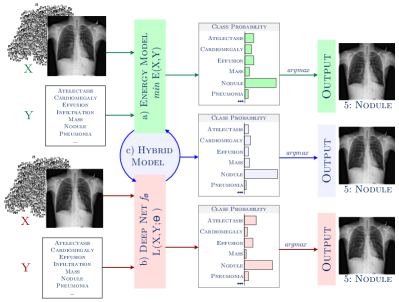
Figure 1: Three major semi-supervised categories in image classification. a) Energy models seek to minimise a given energy (a maximum in probability) to infer the labels for the unlabelled set. b) Deep learning techniques aim to predict the unlabelled samples solely relying on deep networks. c) Hybrid techniques use principles from both energy models and deep networks.

2 Related Work

The problem of classifying images with scarce annotations has been extensively investigated in the machine learning community. In the literature, semi-supervised learning (SSL) can be broadly divided into three categories: energy models (classic techniques) e.g. [5, 6, 10, 11], deep-learning based methods e.g. [16, 17, 18, 31], and hybrid techniques e.g. [19, 20, 21]. An illustration of each category is displayed in Fig. 1. These categories can be split by different perspectives including graph-based techniques, generative models, pseudo-labelling and consistency regularisation. In this section, we review the existing techniques.

Energy Models for Semi-Supervised Classification. Semi-supervised classification has been extensively investigated in the literature, where the underpinning theory of this paradigm has been actively developed since early works e.g. [32, 33, 34, 35, 3]. The solid foundations have been strongly driven by the practical interest of relying less on labelled data in real-world applications such as text analysis [36, 35]. A first family of techniques developed in the area is the energy models [3, 5, 6], where the main idea is to minimise a given energy (a maximum in probability) to infer the labels from the huge amount of unlabelled data using as prior a tiny labelled set. An illustration of this class of techniques is displayed in Fig. 1-a. The term energy models has been largely used in mathematics and physics for years, and since the early developments in semi-supervised learning e.g. [3, 5, 6]. There are several perspectives under this family of techniques including generative models e.g. [37, 38, 39] and low-density separation approaches e.g. [40, 35, 41, 42]. Besides these techniques another large subfamily of techniques is graph based approaches which is the focus of our interest.

Several techniques have been reported following the graph perspective including random walks e.g. [43, 44], harmonic based energy e.g. [5], graph mincut e.g. [45, 9, 46], and spectral techniques e.g [47, 48]. In most recent works, the authors of [49] used a sparse variant of label propagation under the condition that initial labels are in the proximity of the cluster boundaries. A weighted nonlocal Laplacian energy was introduced in [50], where the authors enforce preservation of the symmetry of the Laplace operator. A kernel clustering approach was used in [51, 52] as an approach for Laplacian regularisation. The Poisson equation on a graph was used in [53] for low label rates classification.

Deep Semi-Supervised Techniques. The power of deep learning has been recently applied for semi-supervised classification, which leads the current state-of-the-art performance. A visualisation of this family of techniques is displayed in Fig. 1-b). There exist two major families of techniques in modern semi-supervised techniques: consistency regularisation (aka perturbation-based methods) e.g. [16, 31, 54] and pseudo-labelling e.g. [55, 29, 56]. Consistency regularisation techniques work under the assumption that the model’s performance (output $g(X_{u})$, where $X_{u}$ is the unlabelled data) should not change under any induced $\tau$-perturbation – that is: $g(X_{u})=g(X_{u}+\tau)$. Following this principle, several techniques have been proposed including the works of [16, 17, 18, 57, 58, 59, 56]. A major challenge on these approaches is how to set $\tau$. Different strategies for $\tau$ have been considered in the literature, including mixup augmentations e.g. [60], generative augmentations e.g. [18] and SOTA augmenters e.g. [61, 62]. The core of the performance, of this family of technique, is the use of costly optimisation schemes (e.g. more than 1M training iterations) along with strong augmentations.

The second large family of deep semi-supervised techniques is pseudo-labelling introduced by Lee in [55]. The idea of pseudo-labelling is to generate proxy labels to guide the learning process. Different techniques have been proposed to improve the performance of pseudo-labelling. The use of mix-max feature regularisation was presented in [63]. The authors of [64] proposed a density aware mechanism for improving feature learning and pseudo-label generation. Label propagation using the graph Laplacian with the $p=2$ case have been proposed in [19] and in combination with clustering regularisation in [20]. Mixup has been shown to offer good performance along with small labels per mini-batch [29], and together with graph based pseudo-labels [21]. Certainty mechanisms have also been proposed to improve pseudo-labelling [30, 56].

Hybrid Techniques and Comparison to our Work. Whilst existing techniques either are energy models or deep learning techniques, works simultaneously using these principles, called  hybrid techniques, are very recent and scarce (see Fig. 1-c). The existing works are under the family of pseudo-labelling techniques, where energy models have been used for improving performance. The work of [19] adapted the energy model of [6] to an inductive framework using modern deep networks. The same energy model was used in [20] along with clustering regularisation. Most recently, the work of [21] showed high performance by using the energy model of [6] along with a multi-sampling augmentation strategy.

The existing hybrid models have a commonality that is the use of the energy model of [6], where one seeks to minimise (2) for the specific case $p=2$. The focus of existing works is not the energy model part but rather the development of mechanisms for improving the network performance. In contrast to those works, our approach centers in developing better energy functionals and their theoretical properties to help the learning process. Moreover, existing works have not investigated how more robust energy models impact the performance.

3 Preliminaries

This work addresses the problem of semi-supervised classification. In particular, we follow the graph based perspective in semi-supervised learning. Formally, we aim at solving the following problem.

Problem Statement. Given a set of samples $X=(x_{1},...,x_{l},x_{l+1},...,x_{n})\text{ where }x_{i}\in\mathcal{X}$, we assume that a tiny subset is labelled $D_{L}=\{(x_{i},y_{i})\}_{i=1}^{l}$ with provided labels $\{y_{i}\}_{i=1}^{l}\in\mathcal{L}=\{1,..,L\}$ for $L$ classes, and a large subset is unlabelled $X_{u}=\{x_{i}\}_{i=l+1}^{n}$ . We then seek to infer a function $f:\mathcal{X}\mapsto\mathcal{L}$ such that $f$ gets a good estimate for $\{x_{i}\}_{i=l+1}^{n}$ with minimum generalisation error.

Figure 2: Visual illustration of our graph based energy that seeks to infer better pseudo-labels. Left figure displays the initial graph where only a tiny label set is given as prior. Each colour represents a different class (few given labels per class, e.g.  =’Mass’,  =’Nodule’, using the ChestXray-14 dataset) and black nodes denotes the unlabelled data. Right side shows the inferred pseudo-labels using our energy model.

We address this problem from the hybrid perspective (see Fig. 1-c), where one seeks to combine principles from energy models and deep networks. In particular, our work focus on a hybrid technique from the pseudo-labelling perspective. In deep semi-supervised classification for pseudo-labelling, the main goal is to solve a loss that relates the labelled and unlabelled sets, whose general form reads:

$$\min_{\theta}{{\sum_{(x,y)\in D_{L}}\mathcal{L_{S}}(x,y;\theta)}}+\gamma{{\sum_{x,\in X_{u}}\mathcal{L_{U}}(x,\hat{y};\theta)}},$$ (1)

where the two terms $\mathcal{L_{S}}$ and $\mathcal{L_{U}}$ handle the labelled and unlabelled set respectively, $\theta$ is the network parameters, $\hat{y}$ are pseudo-labels, and $\gamma$ a positive parameter weighting the importance of each term. In the body of literature, the main difference between existing works is the way to define $\mathcal{L_{U}}$, for example using a pseudo-labelling strategy or consistency regularisation.

A current major challenge is how to better handle issues relating to network calibration and confirmation bias e.g. [26, 27, 28, 29]. In the context of pseudo-labelling, hybrid techniques e.g. [19, 20, 21] have shown that one can mitigate such issues by inferring pseudo-labels from an energy model and then combine them with deep networks rather than predict them directly from a deep network. However, existing hybrid techniques have only focused on designing mechanism for the networks and the investigation of better energy models are to be investigated.

With previous motivation in mind, we seek to design better funtionals for improving the inference of pseudo-labels. To do this, we follow a graph based perspective for inferring more certain pseudo-labels. In this work, we consider functions $u\in{\mathbb{R}}^{n}$, defined over a set $\mathcal{N}$ of $n$ nodes. Our main points of interest are convex and absolutely $p$-homogeneous (i.e. $J(\alpha u)=|\alpha|^{p}J(u)$) non-local functionals, defined on $u$, of the particular form:

$$D_{p}(u)=\sum_{ij}w_{ij}\left|\left|\frac{u_{i}}{d_{i}^{1/p}}-\frac{u_{j}}{d_{j}^{1/p}}\right|\right|^{p},$$ (2)

with weights $w_{ij}=w_{ji}\geq 0$ taken such that the vector $d\in{\mathbb{R}}^{n}$ has non-null entries satisfying: $d_{i}=\sum_{j}w_{ij}>0$. This energy acts on the graph defined by nodes $\mathcal{N}$ and weights $w_{ij}$. With respect to classical Dirichlet energies associated to the graph $p$-Laplacian [65, 66, 23, 24], it includes a normalisation through rescaling with the degree of the node. In this work, we focus our attention to the non smooth case $p=1$ with the absolutely one homogeneous energy defined by the function $J(u)=D_{1}(u)$ that can be rewritten as:

$$J(u)=|\!|WD^{-1}u|\!|_{1},$$ (3)

with an $n\times n$ diagonal matrix $D=\operatorname{diag}(d)$, containing the nodes degree so that $d=D\mathbf{1}_{n}$, and an $m\times n$ matrix $W$ that encodes the $m$ edges in the graph. Each of these edges is represented on a different line of the sparse matrix $W$ with the value $w_{ij}$ (resp. $-w_{ij}$) on the column $i$ (resp. $j$).

Subdifferential. Let us first define as $\partial J$ the set of possible subdifferentials of $J$: $\partial J=\{\phi,\,\textrm{ s.t. }\exists u,\,\textrm{ with }\phi\in\partial J(u)\}$. Any absolutely one homogeneous function $J$ checks:

$$\begin{split}J(u)&=\sup_{\phi\in\partial J}\langle\phi,u\rangle\\ \end{split}$$ (4)

so that $J(u)=\langle\phi,u\rangle,\,\forall\phi\in\partial J(u)$.

For the particular function $J$ defined in (3), we can observe that

$$\phi\in\partial J\Leftrightarrow\phi=D^{-1}W^{\top}z,\,\textrm{ with }||z||_{\infty}\leq 1.$$ (5)

Considering the finite dimension setting, there exists $L_{J}<\infty$ such that $|\!|\phi|\!|_{2}<L_{J}$, $\forall\phi\in\partial J$. We also have the following property.

Proposition 1.

For all $\phi\in\partial J$, with $J$ defined in (3), one has

$$\langle\phi,d\rangle=0.$$

Proof.

Observing that $d=D\mathbf{1}$ and using (5) we have that $\exists z\in{\mathbb{R}}^{m}$ such that

$$\langle\phi,d\rangle=\langle D^{-1}W^{\top}z,D\mathbf{1}_{n}\rangle.$$

Since the weights satisfy $w_{ij}=w_{ji}$, then for all $z\in{\mathbb{R}}^{m}$:

$$\begin{split}&\langle W^{\top}z,\mathbf{1}_{n}\rangle=\sum_{i}\sum_{j}w_{ij}(z_{i}-z_{j})=\\ &\sum_{i}\sum_{j>i}w_{ij}(z_{i}-z_{j}-z_{i}+z_{j})=0.\end{split}$$

∎

Eigenfunctions. Eigenfunctions of any convex functional $J$ satisfy $\lambda u\in\partial J(u)$. For $J$ being the nonlocal total variation, (i.e. when $d_{i}$ is constant), eigenfunctions are known to be essential tools to provide a relevant clustering of the graph [25]. Methods [22, 67, 68, 69, 70] have thus been designed to estimate such eigenfunctions through the local minimisation of the Rayleigh quotient, which reads:

$$\min_{|\!|u|\!|_{2}=1}\frac{J(u)}{H(u)},$$ (6)

with another absolutely one homogeneous function $H$, that is typically a norm. Taking $H(u)=|\!|u|\!|_{2}$ as the $\ell_{2}$ norm, one can recover eigenfunctions of $J$. For $H(u)=|\!|u|\!|_{1}$ being the $\ell_{1}$ norm, one can also compute bi-valued functions $u$ that are local minima of (6) and eigenfunctions of $J$ [71]. Being bivalued, these estimations can easily be used to realise a partition of the domain. These schemes also relate to the Cheeger cut of the graph induced by nodes $u_{i}$ and edges $w_{ij}$. Balanced cuts can also be obtained by considering $H(u)=|\!|u-\operatorname{median}(u)|\!|_{1}$ [24].

A last point to underline comes from Proposition 1 that states that eigenfunctions $\lambda u\in\partial J(u)$ should be orthogonal to $d$. It is thus important to design schemes that ensure this property.

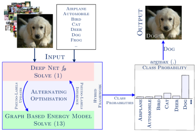
Figure 3: Visual illustration of our hybrid framework. The core of our technique is a graph based energy model for inferring better pseudo-labels (see green box). These are then updated in an alternating optimisation fashion through a deep net (red box) for boosting the classification performance. The output is assigned as the one with the highest probability.

4 Improving Pseudo-Labelling with the 1-Laplacian Graph Energy

This section describes our proposed energy model that fits into a hybrid framework that we called CREPE Model (1-LaplaCian gRaph Energy for Pseudo-labEls). As illustrated in Fig. 3, there are two main components in hybrid techniques: a deep network and an energy model. In this work and unlike existing hybrid techniques that focused on designing better mechanisms for improving the network performance, we focus on developing better energy functionals and their theoretical properties (see green box from Fig. 3). This section describes three key parts: i) the convergence of our energy model, ii) the definition of our coupling constrain for the multi-class problem and iii) our multi-class energy flow for pseudo-labelling.

Core Idea. We seek to infer better pseudo-labels using an energy model (outside a deep network) instead of generating them directly from a deep network. To do this, we introduce a 1-Laplacian graph energy (see green box from Fig. 3), which is detailed next.

4.1 Convergence Analysis

In the following, we will denote the value of function $u$ at node $x$ by $u(x)$ and the value of $u$ at iteration $k$ as $u_{k}$. In order to realise a binary partition of the domain of the graph $\mathcal{N}$ through the minimisation of the quotient $R(u)=J(u)/H(u)$, we adapt the method of [71] to incorporate the scaling $d(x)$ of (3) and consider the semi-explicit scheme:

$$\left\{\begin{array}[]{ll}\frac{u_{k+1/2}-u_{k}}{\delta t}&=\frac{J(u_{k})}{H(u_{k})}(q_{k}-\tilde{q}_{k})-\phi_{k+1/2},\\ u_{k+1}&=\frac{u_{k+1/2}}{|\!|u_{k+1/2}|\!|_{2}}\end{array}\right.$$ (7)

with $\phi_{k+1/2}\in\partial J(u_{k+1/2})$, $q\in\partial H(u_{k})$, $\tilde{q}_{k}=\frac{\langle d,q_{k}\rangle}{\langle d,d\rangle}d$. We recall that both $J$ and $H$ are absolutely one homogeneous and satisfy (4). Since $\langle\phi,d\rangle=0$, $\forall\phi\in\partial J$, the shift with $\tilde{q}_{k}$ is necessary to show the convergence of the scheme (7) as we have $u_{k}\to u^{*}\Rightarrow\frac{J(u^{*})}{H(u^{*})}(q^{*}-\tilde{q}^{*})=\phi^{*}$, for $\phi^{*}\in\partial J(u^{*})$ and $q^{*}\in\partial H(u^{*})$.
Such sequence $u_{k}$ satisfies the following properties.

Proposition 2.

For $\langle u_{0},d\rangle=0$, the trajectory $u_{k}$ given by (7) satisfies:

1. $\langle u_{k+1},d\rangle=0$,

2. $||u_{k+1/2}||_{2}\geq||u_{k}||_{2}$,

3. $R(u_{k})$ is non increasing,

4. $H(u_{k+1/2})\leq\kappa<+\infty$.

Proof.

In this proof, we use the fact that $u_{k+1/2}$ defined in (7) is the unique minimiser of:

$$F_{k}(u)=\frac{1}{2\delta t}|\!|u-u_{k}|\!|_{2}^{2}+R(u_{k})\langle q_{k}-\tilde{q}_{k},u\rangle+J(u).$$ (8)

For $\langle u_{k},d\rangle=0$, we have

$$\begin{split}\langle u_{k+1/2},d\rangle&=\langle u_{k},d\rangle+\delta t\left(R(u_{k})\langle(q_{k}-\tilde{q}_{k}),d\rangle-\langle\phi_{k+1/2},d\rangle\right)\\ &=\delta tR(u_{k})\left(\langle q_{k},d\rangle-\frac{\langle d,q_{k}\rangle}{\langle d,d\rangle}\langle d,d\rangle\right)\\ &=0,\end{split}$$

where we used Proposition 1 in the right part of the previous relation to get $\langle\phi_{k+1/2},d\rangle=0$. We conclude with the fact that $u_{k+1}$ is a rescaling of $u_{k+1/2}$.

Since $H$ is a norm, it is absolutely one homogeneous and $q_{k}\in\partial H(u_{k})\Rightarrow H(u_{k})=\langle q_{k},u_{k}\rangle$. Next, we observe that $J(u_{k})=\sup_{\phi\in\partial J}\langle\phi,u_{k}\rangle\geq\langle\phi_{k+1/2},u_{k}\rangle$ and we get

$$\begin{split}\langle u_{k+1/2},u_{k}\rangle&=||u_{k}||^{2}_{2}+\delta t\left(R(u_{k})\langle q_{k}-\tilde{q}_{k},u_{k}\rangle-\langle\phi_{k+1/2},u_{k}\rangle\right)\\ &\geq||u_{k}||^{2}_{2}+\delta t\left(J(u_{k})-R(u_{k})\langle\tilde{q}_{k},u_{k}\rangle-J(u_{k})\right)\\ &\geq||u_{k}||^{2}_{2}-\delta tR(u_{k})\frac{\langle d,q_{k}\rangle}{\langle d,d\rangle}\langle d,u_{k}\rangle\\ &\geq||u_{k}||^{2}_{2}.\end{split}$$

We then conclude with the fact that $\langle u_{k+1/2},u_{k}\rangle\leq||u_{k+1/2}||_{2}.||u_{k}||_{2}$.

Since $\langle u_{k},d\rangle=0$ for all $k$ and $\tilde{q}_{k}=\frac{\langle d,q_{k}\rangle}{\langle d,d\rangle}d$, then $\langle\tilde{q},u_{k+1/2}\rangle=\langle\tilde{q},u_{k}\rangle=0$. Next, we recall that $H(u_{k+1/2})=\sup_{q\in\partial H{.}}\langle q,u_{k+1/2}\rangle\geq\langle q_{k},u_{k+1/2}\rangle$. Hence we have

$$\begin{split}F_{k}(u_{k+1/2})\leq F(u_{k})\\ \frac{1}{2\delta t}|\!|u_{k+1/2}-u_{k}|\!|_{2}^{2}-R(u_{k})\langle q_{k},u_{k+1/2}\rangle+J(u_{k+1/2})\leq 0\\ \frac{1}{2\delta t}|\!|u_{k+1/2}-u_{k}|\!|_{2}^{2}+J(u_{k+1/2})\leq R(u_{k})H(u_{k+1/2})\\ R(u_{k+1/2})\leq R(u_{k})\\ R(u_{k+1})\leq R(u_{k})\\ \end{split}$$ (9)

where the final rescaling with $|\!|u_{k+1/2}|\!|_{2}$ is possible since $J$ and $H$ are absolutely one homogeneous functions.

In the finite dimension setting, there exists $K_{J},K_{H}<\infty$ such that $||p||\leq K_{J}$ and $||q||\leq K_{H}$ for an absolutely one homogeneous functionals $J$ defined in (1) and a norm $H$. Then one has

$$\begin{split}u_{k+1/2}&=u_{k}+\delta t\left(\frac{J(u_{k})}{H(u_{k})}(q_{k}-\tilde{q}_{k})-\phi_{k+1/2}\right)\\ |\!|u_{k+1/2}|\!|_{2}^{2}&=\langle u_{k},u_{k+1}\rangle+\delta t\left(\frac{J(u_{k})}{H(u_{k})}\langle q_{k},u_{k+1/2}\rangle-\langle\phi_{k+1/2}\rangle\right)\\ |\!|u_{k+1/2}|\!|_{2}^{2}&\leq|\!|u_{k+1/2}|\!|_{2}\left(|\!|u_{k}|\!|_{2}+\delta t\left(\frac{J(u_{k})}{H(u_{k})}K_{H}+K_{J}\right)\right)\\ |\!|u_{k+1/2}|\!|_{2}&\leq 1+\delta t\left(\frac{J(u_{0})}{H(u_{0})}K_{H}+K_{J}\right).\end{split}$$

From the equivalence of norms in finite dimensions, there exists $0<\kappa<\infty$ such that $H(u_{k+1/2})\leq\kappa$. ∎

Hence, we can show the convergence of the trajectory.

Proposition 3.

The sequence $u_{k}$ defined in (7) converges to a non-constant steady point $u^{*}$.

Proof.

As $u_{k+1/2}$ is the unique minimiser of $F_{k}$ in (8), as $F_{k}(u_{k})=0$, and as $\langle q_{k}-\tilde{q}_{k},u_{k+1/2}\rangle\leq H(u_{k+1/2})$, we get:

$$\frac{1}{2\delta tH(u_{k+1/2})}|\!|u_{k+1/2}-u_{k}|\!|_{2}^{2}+R(u_{k+1})\leq R(u_{k}).$$ (10)

Since $u_{k+1}$ is the orthogonal projection of $u_{k+1/2}$ on the $\ell_{2}$ ball then $|\!|u_{k+1}-u_{k}|\!|_{2}\leq|\!|u_{k+1/2}-u_{k}|\!|_{2}$. Finally, from statement 4 of Proposition 2, we have that $1/H(u_{k+1/2})\geq 1/\kappa$. We then sum relation (10) from $0$ to $K$ and deduce that:

$$\sum_{k=0}^{K}\frac{1}{2\delta t\kappa}|\!|u_{k+1}-u_{k}|\!|_{2}^{2}\leq H(u_{0}),$$

so that $|\!|u_{k+1}-u_{k}|\!|_{2}$ converges to $0$. Since all the quantities are bounded, we can show that up to a subsequence $u_{k}\to u^{*}$ (see [71], Theorem 2.1).

From Proposition 2, the points $u_{k}$ being of constant norm and $\langle d,u_{k}\rangle$ being zero (with positive weights $d_{i}$), the limit point $u^{*}$ of the trajectory (7) necessarily has negative and positive entries. ∎

In practice, to realise a partition of the graph with the scheme (7), we miniminise the functional (8) at each iteration $k$ with the primal-dual algorithm of [72] to obtain $u_{k+1/2}$, and then normalise this estimation. As it is non-constant and satisfies $\langle u^{*},d\rangle=0$, the limit of the scheme $u^{*}$ can be used for partitioning with the simple criteria $u^{*}>0$.

4.2 Our Coupling Constraint

As we consider a multi-class setting, we aim at finding $L$ coupled functions $u^{l}$ that are all local minima of the ratio $J(u)/H(u)$. The issue is to define a coupling constraint between the $u^{l}$’s such that it is easy to project on. Let ${\bf u}=[u^{1},\cdots u^{L}]$, in this work we consider the following simple linear coupling, which reads:

$$C:\{{\bf u},\,\textrm{s.t. }\sum_{l=1}^{L}u^{l}(x)=0,\,\forall x\in\mathcal{N}\}.$$ (11)

There are three main reasons for considering such coupling instead of classical simplex [24, 73, 74] or orthogonality [75] constraints:

1. Projection on this linear constraint is explicit with a simple shift of the vector ${\bf u}(x)$ for each node $x$. On the other hand, simplex constraint ($u^{l}(x)\geq 0$, $\sum_{l}u^{l}(x)=1$, $\forall x$) requires more expensive projections of the vectors ${\bf u}(x)$ on the $L$ simplex. Lastly, projection on the orthogonal constraint of the $u^{l}$’s is a non convex problem.

2. Contrary to the simplex constraint, it is compatible with the weighted zero mean condition $\langle u^{l},d\rangle$ that any eigenfunction of $J$ should satisfy, as shown in Proposition 1.

3. The characteristic function of a linear constraint is absolutely one homogeneous. This leads to a natural extension of the binary case.

4.3 Multi-Class Flow for Better Pseudo-Labelling

In previous section, we provide the convergence analysis and coupling constraint of our energy model. In this section, we detail how these elements fit into our new energy functional for pseudo-labelling.

We recall to the reader that we consider the problem:

$$\min_{|\!|{\bf u}|\!|_{2}=1}\sum_{l=1}^{L}\frac{J(u^{l})}{H(u^{l})}.$$ (12)

To find a local minima of (12), we define our iterative multi-class energy functional, which reads:

$$F^{L}_{k}({\bf u})=\frac{1}{2\delta t}|\!|{\bf u}-{\bf u}_{k}|\!|_{2}^{2}-\sum_{l=1}^{L}R(u_{k}^{l})\langle q_{k}^{l}-\tilde{q}_{k}^{l},u^{l}\rangle\\ +\sum_{l=1}^{L}J(u^{l})+\chi_{C}({\bf u})$$ (13)

where $q_{k}^{l}\in\partial H(u_{k}^{l})$ and $\chi_{C}$ is the characteristic function of the constraints (11). Starting from an initial point ${\bf u}_{0}$ that satisfies the constraint ($\chi_{C}({\bf u}_{0})=0$) and has been normalised ($|\!|{\bf u}_{0}|\!|_{2}^{2}=\sum_{l=1}^{L}|\!|u_{0}^{l}|\!|_{2}^{2}=1$), the scheme we consider reads:

$$\left\{\begin{array}[]{ll}{\bf u}_{k+1/2}&=\underset{{\bf u}}{\operatorname{argmin}}\;F^{L}_{k}({\bf u})\vspace{0.2cm}\\ {\bf u}_{k+1}&=\frac{{\bf u}_{k+1/2}}{|\!|{\bf u}_{k+1/2}|\!|_{2}}.\end{array}\right.$$ (14)

In practice, if for some $l$, $u^{l}_{k+1/2}$ vanishes, then we define $R(u^{l}_{k+1})=0$ for the next iteration. With such assumptions, the sequence ${\bf u}_{k}$ have the following properties.

Proposition 4.

For $\langle u_{0}^{l},d\rangle=0$, $l=1\cdots L$, the trajectory ${\bf u}_{k}$ given by (14) satisfies

1. $\langle u_{k}^{l},d\rangle=0$,

2. $||{\bf u}_{k}||_{2}\leq||{\bf u}_{k+1/2}||_{2}\leq\kappa<\infty$,

3. $\sum_{l=1}^{L}H(u_{k+1}^{l})\left(R(u_{k+1}^{l})-R(u_{k}^{l})\right)$
                     $\leq-\frac{1}{2\delta t\kappa}|\!|{\bf u}_{k+1}-{\bf u}_{k}|\!|_{2}^{2}$.

Proof.

The scheme reads

$$\left\{\begin{array}[]{ll}{\bf u}_{k+1/2}=\underset{{\bf u}}{\operatorname{argmin}}\;F^{L}_{k}({\bf u}):=\frac{1}{2\delta t}|\!|{\bf u}-{\bf u}_{k}|\!|_{2}^{2}+\sum_{l=1}^{L}J(u^{l})\\ \hskip 14.22636pt-\sum_{l=1}^{L}R(u_{k}^{l})\langle q_{k}^{l}-\tilde{q}_{k}^{l},u^{l}\rangle+\chi_{C}({\bf u})\vspace{0.3cm}\\ {\bf u}_{k+1}=\frac{{\bf u}_{k+1/2}}{|\!|{\bf u}_{k+1/2}|\!|_{2}}.\end{array}\right.$$

The Karush–Kuhn–Tucker conditions of the above problem states that there exist $\phi^{l}_{k+1/2}$ and $r_{k+1/2}$ such that

$$u_{k+1/2}^{l}=u_{k}^{l}+\delta t\left(R(u^{l}_{k})(q_{k}^{l}-\tilde{q}^{l}_{k})-\phi^{l}_{k+1/2}-r_{k+1/2}\right)$$

where $\phi^{l}_{k+1/2}\in\partial J(u^{l}_{k+1/2})$ and $r_{k+1/2}$ is a Lagrange multiplier independent of $l$ for the linear constraint $\chi_{C}$. The point ${\bf u}_{k+1/2}$ in the above scheme corresponds to the global minimiser of $F^{L}_{k}({\bf u})$.

For $\langle u^{l}_{k},d\rangle=0$, and following point 1 of Proposition 2, we have

$$\begin{split}\langle u_{k+1/2}^{l},d\rangle&=\langle u_{k}^{l},d\rangle+\delta t\big{(}R(u_{k}^{l})\langle(q_{k}^{l}-\tilde{q}_{k}^{l}),d\rangle\\ &-\langle\phi^{l}_{k+1/2},d\rangle-\langle r_{k+1/2},d\rangle\big{)}\\ &=-\langle r_{k+1/2},d\rangle.\end{split}$$

Next, as ${\bf u}_{k+1/2}\in C$, we have $\sum_{l}u^{l}_{k+1/2}(x)=0$, $\forall x\in\mathcal{N}$ and obtain:

$$\begin{split}\sum_{l=1}^{L}\langle u_{k+1/2}^{l},d\rangle&=-\sum_{l=1}^{L}\langle r_{k+1/2},d\rangle\\ \sum_{l=1}^{L}\sum_{x\in\mathcal{N}}u^{l}_{k+1/2}(x)d(x)&=-L\langle r_{k+1/2},d\rangle\\ \sum_{x\in\mathcal{N}}d(x)\left(\sum_{l=1}^{L}u^{l}_{k+1/2}(x)\right)&=-L\langle r_{k+1/2},d\rangle\\ 0&=\langle r_{k+1/2},d\rangle.\end{split}$$

We have

$$\begin{split}\langle u^{l}_{k+1/2},u^{l}_{k}\rangle=||u^{l}_{k}||^{2}_{2}+\delta t\left(R(u^{l}_{k})\langle q^{l}_{k}-\tilde{q}^{l}_{k},u^{l}_{k}\rangle-\right.\\ \left.\langle\phi^{l}_{k+1/2},u^{l}_{k}\rangle-\langle r_{k+1/2},u^{l}_{k}\rangle\right).\end{split}$$

We follow the point 2 of Proposition 2 to first get: $\langle u_{k+1/2}^{l},u_{k}^{l}\rangle\geq|\!|u_{k}^{l}|\!|_{2}-\langle r^{l}_{k+1/2},u_{k}^{l}\rangle$, for $i=1\cdots n$. Then, as $\sum_{l}\langle r_{k+1/2},u^{l}_{k}\rangle=\sum_{x}r_{k+1/2}(x)\sum_{l}u^{l}_{k}(x)=0$, we deduce that $|\!|{\bf u}_{k+1/2}|\!|_{2}.|\!|{\bf u}_{k}|\!|_{2}\geq\sum_{l}\langle u^{l}_{k+1/2},u^{l}_{k}\rangle\geq\sum_{l}\langle u^{l}_{k},u^{l}_{k}\rangle=||{\bf u}_{k}||_{2}^{2}$. Next we observe that

$$\begin{split}|\!|u^{l}_{k+1/2}|\!|_{2}^{2}&=\langle u^{l}_{k+1/2},u^{l}_{k}\rangle+\delta t\left(-\langle r_{k+1/2},u^{l}_{k+1/2}\rangle\right.\\ &\left.+R(u^{l}_{k})\langle q^{l}_{k}-\tilde{q}^{l}_{k},u^{l}_{k+1/2}\rangle-J(u^{l}_{k+1/2})\right).\end{split}$$

Summing on $l$, we get

$$\begin{split}|\!|{\bf u}_{k+1/2}|\!|_{2}^{2}&\leq|\!|{\bf u}_{k+1/2}|\!|_{2}\left(|\!|{\bf u}_{k}|\!|_{2}+\delta t\left(\sum_{l=1}^{L}R(u^{l}_{k})|\!|q_{k}^{l}|\!|_{2}\right.\right.\\ &\left.\left.+|\!|\phi^{l}_{k+1/2}|\!|_{2}\right)\right)\\ |\!|{\bf u}_{k+1/2}|\!|_{2}&\leq|\!|{\bf u}_{k}|\!|_{2}+\delta t\left(\sum_{l=1}^{L}\frac{J(u^{l}_{k})}{H(u^{l}_{k})}K_{H}+K_{J}\right)\leq 1\\ &+\delta tK_{J}\left(\sum_{l=1}^{L}\frac{|\!|u^{l}_{k}|\!|_{2}}{H(u^{l}_{k})}K_{H}+1\right).\end{split}$$

Notice that we defined $R(u^{l}_{k})=0$ for $u^{l}_{k}=0$. As $H$ is a norm, the equivalence of norm in finite dimensions implies that ${|\!|u^{l}_{k}|\!|_{2}}{H(u^{l}_{k})}$ is bounded by some constant $c<\infty$. We then have $|\!|{\bf u}_{k+1/2}|\!|_{2}\leq\kappa=1+\delta tK_{J}\left(1+LK_{H}c\right)$.

Since ${\bf u}_{k+1/2}$ is the global minimiser of (10), then:

$$\begin{split}&\hskip 85.35826ptF_{k}^{L}({\bf u}_{k+1/2})\leq F_{k}^{L}({\bf u}_{k})\\ &\frac{1}{2\delta t}|\!|{\bf u}_{k+1/2}-{\bf u}_{k}|\!|_{2}^{2}+\sum_{l=1}^{L}J(u^{l}_{k+1/2})\leq\sum_{l=1}^{L}R(u_{k}^{l})\langle q_{k}^{l}-\tilde{q}_{k}^{l},u^{l}_{k+1/2}\rangle\\ &\frac{1}{2\delta t}|\!|{\bf u}_{k+1/2}-{\bf u}_{k}|\!|_{2}^{2}+\sum_{l=1}^{L}J(u^{l}_{k+1/2})\leq\sum_{l=1}^{L}R(u_{k}^{l})H(u_{k+1/2}^{l})\\ &\sum_{l=1}^{L}\left(J(u^{l}_{k+1/2})-\frac{J(u_{k}^{l})}{H(u_{k}^{l})}H(u_{k+1/2}^{l})\right)\leq-\frac{1}{2\delta t}|\!|{\bf u}_{k+1/2}-{\bf u}_{k}|\!|_{2}^{2}\\ &|\!|{\bf u}_{k+1/2}|\!|_{2}\sum_{l=1}^{L}H(u_{k+1}^{l})\left(R(u_{k+1}^{l})-R(u_{k}^{l})\right)\leq-\frac{1}{2\delta t}|\!|{\bf u}_{k+1}-{\bf u}_{k}|\!|_{2}^{2}\\ &\sum_{l=1}^{L}H(u_{k+1}^{l})\left(R(u_{k+1}^{l})-R(u_{k}^{l})\right)\leq-\frac{1}{2\delta t\kappa}|\!|{\bf u}_{k+1}-{\bf u}_{k}|\!|_{2}^{2}.\qed\end{split}$$

Point 3 of Proposition 4 contains weights $H(u_{k+1}^{l})$ that prevent from showing the exact decrease of the sum of ratios. This is in line with the results in [24]. To ensure the decrease of the sum of ratios $\sum_{l=1}^{L}{J(u^{l}_{k})}/{H(u^{l}_{k})}$, it is possible to introduce auxiliary variables to deal with individual ratio decrease, as in [73]. The involved sub-problem at each iteration $k$ is nevertheless more complex to solve.

4.4 Introducing Label Priors

The partitioning process induced by the scheme (14) so far does not integrate any label information. As we are working in a semi-supervised setting, we consider given a small subsets of labelled nodes $\mathcal{N}^{l}\subset\mathcal{N}$ (with $|\mathcal{N}^{l}|<<|\subset\mathcal{N}|$) belonging to each cluster $i$, with $\mathcal{N}^{l}\cap\mathcal{N}_{j}=\emptyset$. Denoting as $\mathcal{L}=\cup_{l=1}^{L}\mathcal{N}^{l}$, the objective is to propagate the prior information in the graph in order to infer pseudo-labels for the remaining nodes $x\in\mathcal{N}\backslash\mathcal{L}$. To that end, we simply have to modify the coupling constraint $C$ in (11) as

$$C:\left\{{\bf u},\,\textrm{s.t. }\begin{array}[]{ll}\sum_{l=1}^{L}u^{l}(x)=0&\textrm{if }x\in\mathcal{N}\backslash\mathcal{L}\\ u^{l}(x)\geq\epsilon&\textrm{if }x\in\mathcal{N}^{l}\\ u^{l^{\prime}}(x)\leq-\epsilon,\forall l^{\prime}\neq l&\textrm{if }x\in\mathcal{L}\backslash\mathcal{N}^{l}\end{array}\right\}.$$ (15)

With such constraint, clusters can no longer vanish or merge since they all contain different active nodes $x\in\mathcal{N}^{l}$ satisfying $u^{l}(x)>0$. The same scheme (14) with the new constraint set (15) can be applied to propagate these labels. Once it has converged, the inferred pseudo-label of each unlabelled node $x\in\mathcal{N}\backslash\mathcal{L}$ is taken as:

$$L(x)\in\underset{i\in\{1,\cdots L\}}{\operatorname{argmax}}\;u^{l}(x).$$ (16)

Soft labelling can either be obtained by considering all the clusters with non negative weights $\mathcal{I}(x)=\{l,\,u^{l}(x)\geq 0\}\neq\emptyset$ and with relative weights $w^{l}(x)=u^{l}(x)/(\sum_{l\in\mathcal{I}(x)}u^{l}(x))$, with the convention that $w^{l}(x)=1/L$, in the case that $u^{l}(x)=0$ for all $l=1\cdots L$ (which has never been observed in our experiments). For notation purposes and following the notation in (1), we denote the output of (16) as $\hat{y_{i}}$, having $\hat{Y}=\{\hat{y}_{k}\}_{k=l+1}^{n}$. The parameter $\epsilon$ in (15) is set to a small numerical value.

4.5 Hybrid Framework

We now fit our energy model into a hybrid framework as displayed in Fig. 3. We perform an alternating optimisation between (1) and (14). The process (14), that provides pseudo-labels $\hat{y}$, is extensively described in previous subsections (as our main contribution). The functional (1) is now detailed. For the first term in (1), we use a cross entropy loss with a weighting parameter as imbalance class strategy. We follow a standard strategy e.g. [76, 77] such that the parameter is inversely proportional to the number of samples for class $k:\beta_{k}\propto 1/\mathcal{E}_{n}$ where $\mathcal{E}_{n}$ is the total number of samples. The second term in (1) involves the inferred pseudo-labels updates $\hat{y}$ in a cross entropy loss, along with a dual weighting parameter $\beta\varphi$ where $\varphi$ is a measure of the uncertainty referring to the entropy. The remaining of the experiments follows this alternating optimisation. The choice for $f_{\theta}$ is discussed in the experimental results section.

5 Experimental Results

This section focuses on the detailed description of the experiments that we conducted to evaluate our proposed approach.

5.1 Data Description

We extensively evaluate our approach using six very diverse datasets. Firstly, we use the Fashion-MNIST [78] dataset. The dataset is composed of 70k grayscale images containing 10 classes from fashion items. To further support the generalisation and robustness of our technique, we use two major complex datasets from the medical domain. The ChestX-ray14 dataset [79] is composed of 112,120 frontal chest view X-ray with size of 1024$\times$1024 and 14 classes reflecting diverse pathologies. The CBIS-DDSM dataset [80], composed of 3,103 mammography images with a mean size of 3138$\times$5220, contains normal, benign, and malignant cases with verified pathology information. Finally, we use three natural image datasets. The CIFAR-10 and CIFAR-100 dataset [81] that contains 60k colour images of size 32$\times$32 with 10 and 100 different classes respectively. Finally, the Mini-ImageNet [82] dataset consisting of 60k colour images with of size $64\times 64$ and 100 classes.

TABLE I: Numerical comparison of our approach vs other energy-based approaches. The values are computed from 20 runs as the average of error rate $\pm$ standard deviation over several label counts. The best results are highlighted green whilst the second best ones are highlighted in red.

	% Labelled Set
Technique	1%	2%	5%	10%	20%	30%
Harmonic Gaussian (HG) [5]	18.97$\pm$0.34	17.96$\pm$0.23	16.35$\pm$0.10	15.33$\pm$0.10	14.48$\pm$0.11	14.09$\pm$0.08
Local to Global Consistency (LGC) [6]	18.65$\pm$0.59	17.81$\pm$0.31	16.41$\pm$0.12	15.20$\pm$0.15	14.33$\pm$0.13	13.68$\pm$0.06
Lazy Random Walks (LRW) [44]	19.09$\pm$0.25	17.84$\pm$0.17	16.38$\pm$0.06	15.69$\pm$0.10	15.35$\pm$0.10	15.19$\pm$0.07
Sparse Label Propagation (SLP) [49]	78.18$\pm$1.37	50.16$\pm$3.81	44.18$\pm$0.37	25.17$\pm$1.75	19.03$\pm$1.75	13.16$\pm$0.11
Weighted Nonlocal Laplacian (WNLL) [50]	19.68$\pm$0.17	18.96$\pm$0.28	17.41$\pm$0.12	16.15$\pm$0.17	14.93$\pm$0.13	14.32$\pm$0.09
Centered Kernel (CK) [51, 52]	31.16$\pm$1.28	24.29$\pm$0.61	20.30$\pm$0.11	18.62$\pm$0.24	16.54$\pm$0.12	15.38$\pm$0.07
Poisson Learning (PoL) [53]	20.60$\pm$1.37	19.89$\pm$3.81	19.17$\pm$0.37	19.03$\pm$1.75	18.82$\pm$0.71	18.87$\pm$0.41
Ours	17.62$\pm$0.21	16.05$\pm$0.24	14.21$\pm$0.08	13.16$\pm$0.11	12.31$\pm$0.09	11.82$\pm$0.04

5.2 Evaluation Protocol

We design the following evaluation scheme to validate our theory.

Baseline Comparison against existing energy models. As the core contribution of this work is a new graph based energy model, we first compared our technique against existing graph-based energy methods: Harmonic Gaussian (HG) [5], Local to Global Consistency (LGC) [6], Lazy Random Walks (LRW) [44], Sparse Label Propagation (SLP) [49], Weighted Nonlocal Laplacian (WNLL) [50], Centered Kernel (CK) [51, 52] and Poisson Learning (PoL) [53]. To solely evaluate the impact of these energy models, we used the same network architecture and substituted each method as the energy model (i.e. only green box of Fig. 3). We run the experiments for all techniques under the same conditions by constructing a k-NN graph with $k=20$ using the features extracted from a 13-Layer Network. We remark that these set of experiments are to purely compare energy models and not networks Fig. 3. We use different label % counts {1,2,5,10,20,30}, and report the mean error and standard deviation over randomly select the labelled samples over twenty repeated times (20 different splits).

Comparison against SOTA Techniques. For our full model we compare to the state-of-the-art for each of the differing domains

Medical Datasets. For the ChestX-ray14 dataset [79], we firstly compared against the SOTA supervised techniques of [79, 83, 84, 85, 86, 87, 88, 89, 90] using the official partition of the dataset (70% labelled data) against ours using 20% of labelled data. Moreover, we compared against the SOTA semi-supervised techniques of [17, 91, 92, 93]. All semi-supervised techniques are reported using 20% of labels. We also provide comparison with existing techniques [80] [94, 95, 96, 97] on the CBIS-DDSM dataset. The quality check is performed following standard convention in the medical domain by a ROC analysis using the area under the curve (AUC).

Natural Image Datasets. Finally, we report results against the SOTA semi-supervised techniques for natural image datasets: $\Pi-$Model and Temporal Ensembling [16], Mean Teacher (MT) [17], VAT [18], $\Pi+$SNTG [98], MT+fast-SWA [57], MT+ICT [58], Dual Student [59], MUSCLE+MT+LP [54], MT+TSSDL [63], MT+LP [19], CycleCluster [20], DAG [64], UPS [30], PL-Mixup [29], LaplaceNet [21], UDA [99], SimPLE [56], FixMatch [31]. We evaluate the quality of the classifiers by reporting the error rate and standard deviation over five runs and for a range number of labelled samples.

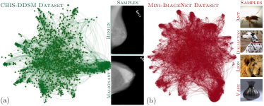
Figure 4: Graph visualisation for two selected datasets used in our experiments. Graphical representation for (a) the CBIS-DDSM dataset and (b) the Mini-ImageNet Dataset. A few sample images for each datasets are displayed at the left side of each graph.

5.3 Implementation Details

We set the architecture for $f_{\theta}$ (i.e. red box of Fig. 3) as follows. For the medical datasets we use a ResNet-18 [2]. For the natural image datasets, we ran experiments with three different networks. For CIFAR-10 and CIFAR-100, we divided our experiments into two parts. For the first part, we use a 13-Layer Network for a fair comparison as existing approaches run under this architecture. For the second part and motivated by the work of [100], we compare against the most recent techniques under exactly the same conditions which includes the optimiser, RandAugment implementation and a WideResNet-28-2 (WRN-28-2). Finally, we use a ResNet-18 for the Mini-Imagenet dataset as fair comparison for existing techniques. For the graph generation, a k-NN graph with $k=20$ is constructed using the features from each respective architecture - Fig. 4 displays examples of generated graphs for two selected datasets. For our approach, we set the number of epochs of 310 and a weight decay of $2\times 10^{-4}$. The learning rate is set to 5e-2 and with a scheduled cosine annealing. We use as optimiser stochastic gradient descent (SGD) and implement our code in PyTorch.

TABLE II: Performance comparison of our approach (20% of labelled data) against SOTA fully-supervised techniques (70% of labelled data). We reported the AUC per class and average AUC over all 14 pathologies. All compared techniques are performed using the official data split. The results in bold denotes the highest performance.

ChestX-ray14	Fully Supervised Techniques (70% Labelled data)									SSL
Pathology	Wang et al [79]	Yao et al [83]	Guendel et al[84]	Shen et al [85]	Baltruschat, [86]	CheXNet [87]	Guan et al[88]	Ma et al [89]	Kim, et al[90]	CREPE (Ours)
Atelectasis	70.03	73.30	76.70	76.60	76.30	75.9	78.10	77.70	78.2	78.65
Cardiomegaly	81.00	85.60	88.30	80.10	87.50	87.1	88.30	89.40	88.1	88.74
Effusion	75.85	80.60	82.80	79.70	82.20	82.1	83.10	82.90	83.6	83.15
Infiltration	66.14	67.30	70.90	75.10	69.40	70.0	69.70	69.60	71.5	72.25
Mass	69.33	77.70	82.10	76.00	82.00	81.0	83.00	83.80	83.4	83.41
Nodule	66.87	71.80	75.80	74.10	74.70	75.9	76.40	77.71	79.9	76.61
Pneumonia	65.80	68.40	73.10	77.80	71.40	71.8	72.50	72.20	73.0	76.04
Pneumothorax	79.93	80.50	84.60	80.00	84.00	84.8	86.60	86.20	87.4	86.89
Consolidation	70.32	71.10	74.50	78.70	74.90	74.1	75.80	75.00	74.7	75.42
Edema	80.52	80.60	83.50	82.00	84.60	84.4	85.30	84.60	83.4	84.96
Emphysema	83.30	84.20	89.50	77.30	89.50	89.1	91.10	90.80	93.6	90.95
Fibrosis	78.59	74.30	81.80	76.50	81.60	81.0	82.60	82.70	81.5	82.16
Pleural Thicken	68.35	72.40	76.10	75.90	76.30	76.8	78.00	77.90	79.8	76.84
Hernia	87.17	77.50	89.60	74.80	93.70	86.7	91.80	93.40	89.6	88.38
Average AUC	74.51	76.09	80.66	77.47	80.57	80.05	81.60	81.71	82.0	81.75

TABLE III: Numerical comparison of our technique and existing semi-supervised approaches for the ChestX-ray14 dataset. All techniques use 20%of labelled data, and the reported results reflect the AUC per class and average. The best results are highlighted green.

ChestX-ray14	Semi-Supervised/Self-Supervised Techniques
Pathology	MT [17]	GraphXNet [91]	MOCOV2 [101, 93]	SRC-MT [92]	S2MTS2 [93]	CREPE (Ours)
Atelectasis	75.12	71.89	77.21	75.38	78.57	78.65
Cardiomegaly	87.37	87.99	85.84	87.70	88.08	88.74
Effusion	80.81	79.20	81.62	81.58	82.87	83.15
Infiltration	70.67	72.05	70.91	70.40	70.68	72.25
Mass	77.72	80.90	81.71	78.03	82.57	83.41
Nodule	73.27	71.13	76.72	73.64	76.60	76.61
Pneumonia	69.17	76.64	71.08	69.27	72.25	76.04
Pneumothorax	85.63	83.70	85.92	86.12	86.55	86.89
Consolidation	72.51	73.36	74.47	73.11	75.47	75.42
Edema	82.72	80.20	83.57	82.94	84.83	84.96
Emphysema	88.16	84.07	91.10	88.98	91.88	90.95
Fibrosis	78.24	80.34	80.96	79.22	81.73	82.16
Pleural Thicken	74.43	75.70	75.65	75.63	76.86	76.84
Hernia	87.74	87.22	85.62	87.27	85.98	88.38
Average AUC	78.83	78.88	80.17	79.23	81.06	81.75

TABLE IV: AUC performance comparison of existing SOTA supervised techniques and our technique for the CBIS-DDSM dataset. The best results are marked in green whilst the second best in red.

CBIS-DDSM Dataset
	Paradigm
Technique	SL (85%)	SSL	AUC
ResNet-34	✓		79.2
Zhu et al [94]	✓		79.1
Tao et al [95]	✓		83.1
Shu et al [96]	✓		83.8
Shen et al$\dagger$ [97]	✓		84.0
CREPE (Ours, 35%)		✓	83.9
CREPE (Ours, 40%)		✓	84.2

TABLE V: Comparison performance of our technique against existing semi-supervised techniques (consistency regularisation and pseudo-labelling family of techniques) along with the fully supervised baseline for CIFAR-10 and CIFAR-100. All the results are derived from using a 13-Layer architecture, and reflect the error rate and standard deviation. The results in bold denotes the best performance.

	Labelled Samples (CIFAR-10)				Labelled Samples (CIFAR-100)
Technique (13-CNN)	1k	2k	4k		4k	10k
Fully Supervised	26.60$\pm$0.22	19.53$\pm$0.12	14.02$\pm$0.10		53.10$\pm$0.34	36.59$\pm$0.47
Consistency Regularisation Techniques
$\Pi-$Model [16]	31.65$\pm$1.20	17.57$\pm$0.44	12.36$\pm$0.31		$-$	39.19$\pm$0.36
Temporal Ensembling [16]	23.31$\pm$1.01	15.64$\pm$0.39	12.16$\pm$0.24		$-$	38.65$\pm$0.51
Mean Teacher (MT) [17]	21.55$\pm$1.48	15.73$\pm$0.31	12.31$\pm$0.28		45.36$\pm$0.49	36.08$\pm$0.51
VAT [18]	$-$	$-$	11.36$\pm$0.34		$-$	$-$
$\Pi+$SNTG [98]	21.23$\pm$1.27	14.65$\pm$0.31	11.00$\pm$0.13		$-$	37.97$\pm$0.29
MT+fast-SWA [57]	15.58$\pm$0.12	11.02$\pm$0.23	9.05$\pm$0.21		$-$	33.62$\pm$0.54
MT+ICT [58]	15.48$\pm$0.78	9.26$\pm$0.09	7.29$\pm$0.02		$-$	$-$
Dual Student [59]	14.17$\pm$0.38	10.72$\pm$0.19	8.89$\pm$0.09		$-$	32.77$\pm$0.24
MUSCLE+MT+LP [54]	13.29$\pm$0.36	$-$	$-$		42.34$\pm$0.45	35.21$\pm$0.25
Pseudo-Labelling Techniques
MT+TSSDL [63]	18.41$\pm$0.92	13.54$\pm$0.32	9.30$\pm$0.55		$-$	$-$
MT+LP [19]	16.93$\pm$0.70	13.22$\pm$0.29	10.61$\pm$0.28		43.73$\pm$0.20	35.92$\pm$0.47
CycleCluster [20]	15.52$\pm$0.88	12.79$\pm$0.35	10.79$\pm$0.45		45.19$\pm$0.34	35.65$\pm$0.50
DAG [64]	7.42$\pm$0.41	7.16$\pm$0.38	6.13$\pm$0.15		37.38$\pm$0.64	32.50$\pm$0.21
UPS [30]	8.18$\pm$0.15	$-$	6.39$\pm$0.02		40.77$\pm$0.10	32.00$\pm$0.49
PL-Mixup [29]	6.85$\pm$0.15	$-$	5.97$\pm$0.15		37.55$\pm$1.09	32.15$\pm$0.50
LaplaceNet [21]	5.33$\pm$0.02	4.99$\pm$0.12	4.64$\pm$0.07		31.64$\pm$0.02	26.60$\pm$0.23
CREPE (Ours)	5.04$\pm$0.03	4.58$\pm$0.11	4.31$\pm$0.08		31.02$\pm$0.03	25.11$\pm$0.19

TABLE VI: Performance comparison using CIFAR-10/100 reporting error rate$\pm$ standard deviation. The consistency regularisation and pseudo-labelling techniques were run under the same code-base using same architecture WRN-28-2.

	Labelled Samples (CIFAR-10)			Labelled Samples (CIFAR-100)
Technique (WRN-28-2)	2k	4k		4k	10k
UDA [99]	5.61$\pm$0.16	5.40$\pm$0.19		36.19$\pm$0.39	31.49$\pm$0.19
FixMatch [31]	5.42$\pm$0.11	5.30$\pm$0.08		34.87$\pm$0.17	30.89$\pm$0.18
SimPLE [56]	5.27$\pm$0.18	5.33$\pm$0.20		34.75$\pm$0.16	29.18$\pm$0.25
LaplaceNet [21]	4.71$\pm$0.05	4.35$\pm$0.10		33.16$\pm$0.22	27.49$\pm$0.22
CREPE (Ours)	4.33$\pm$0.09	4.16$\pm$0.11		32.21$\pm$0.18	26.14$\pm$0.24

TABLE VII: Error rate ($\pm$ standard deviation) comparison for Mini-ImageNet dataset. All techniques use a ResNet-18 Network. Numbers in bold indicate best performance.

	Labelled Samples (Mini-ImageNet)
Technique	4k	10k
Mean Teacher (MT) [17]	72.51$\pm$0.22	57.55$\pm$1.11
LP [19]	70.29$\pm$0.81	57.58$\pm$1.47
Two Cycle Learning [20]	69.12$\pm$1.05	54.27$\pm$0.71
PL-Mixup [29]	56.49$\pm$0.51	46.08$\pm$0.11
SimPLE [56]	50.21$\pm$0.42	43.44$\pm$0.12
LaplaceNet [21]	46.32$\pm$0.27	39.43$\pm$0.09
CREPE (Ours)	45.61$\pm$0.25	38.33$\pm$0.11

5.4 Results & Discussion.

In this section, we report and discuss the results and comparison of our proposed technique.

How Good is our Energy Model? We start by evaluating the performance of our energy model. To do this, we ran a set of comparisons of our technique against existing energy models including recent ones. For a fair comparison all techniques were fed with the same graph (constructed as detailed in previous subsection). The results are displayed in Table I, which reports the error rate averaged over 20 runs and the standard deviation under different % of labelled data. In a closer look at the results, we can observe that our approach reports the lowest error rate for all label counts whilst LGC [6] ranked second. The techniques of CK [51] and SLP [49] failed to be robust in the low label regime and needed a higher number of labels to improve the performance than the compared techniques. A similar performance behaviour was observed in the techniques of HG [5], LGC [6], LRW [44] and WNLL [50]. In contrast to the compared techniques, the performance of PoL [53] was not improved when more labels are considered. Our technique reported a percentage of improvement in the range of 6% to 14% with respect to LGC, the second best ranked technique. Overall and from the results, we highlight a key strength of our energy approach – it demonstrates a good generalisation performance in the low regime labelled set, and consistent performance improvement when more labels are considered.

Hybrid Semi-Supervised Medical Image Classification. We now evaluate our full hybrid framework (see Fig. 3). We start by using the ChestX-ray14 benchmarking dataset [79]. We first compared our approach against the SOTA supervised techniques, they assume a large corpus of annotated data (70%) whilst our technique reports the performance using 20% of labels. The results are reported in Table II displaying the AUC per class and the average over all classes. By inspection we can observe that our technique readily competes with existing deep supervised techniques in per class performance. Overall, our technique outperformed almost all existing techniques and places second behind the work of [90]. However, we remark that our technique is using far less labels (only 20%) than all compared techniques (fully supervised 70% of labelled data).

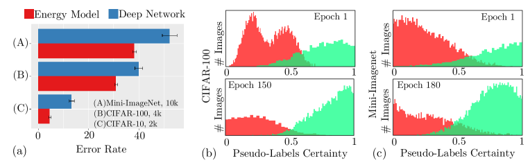
Figure 5: (a) Error rate comparison for pseudo-label generation between our energy model vs the deep network for Mini-Imagenet, CIFAR-10/100. (b)-(c) Certainty $\varphi$ of the pseudo-labels correctness (green) along with those incorrect (red) for two selected epochs for CIFAR-100 (4k labels) and Mini-Imagenet (10k labels) correspondingly.

Figure 6: Average AUC comparison of hybrid models performance using our energy model (red line) and that of [6] (blue line). (a) reports the comparison performance for different % of labels for the ChestX-ray14 dataset whilst b) for the CBIS-DDSM dataset.

We also compared our proposed technique against existing semi-supervised models for medical imaging. The results are reported in Table IV. All results are produced using 20% of labelled data, and the table displays the AUC per class and average over all classes. We observe that our technique reports the best AUC per class in majority of the pathologies, whith a best overall score (see scores highlighted in green). We further support the performance of our method with another challenging medical dataset the CBIS-DDSM dataset [80] for mammograms classification. We compare our approach against existing techniques for such dataset and report the results in Table IV. The compared techniques are deep supervised techniques, and to the best of our knowledge, there exists no modern semi-supervised techniques for this dataset to compare with. For the supervised techniques the official partition is used (i.e. 85% of labelled data). For our technique, we reported the AUC as result of an average of 5 split runs using 35% and 40% of labelled data. From the results, our technique produced readily compared performance whilst using only a fraction of labels, and reported the highest AUC using less than half of the labels than the compared techniques.

Comparison with SOTA Semi-Supervised Models. For our final set of experiments, we compared our technique against existing semi-supervised techniques for natural images where numerous methods have been proposed. For a fair comparison, we first provide a comparison using a 13-Layer Network, which is the most widely used network in semi-supervised classification. The results, in terms of error rate, are presented in Table V. We observe that our technique provides a substantial improvement in performance with respect to consistency regularisation techniques for both CIFAR-10/100 datasets. In terms of existing pseudo-labelling techniques, our technique provides a significant margin of improvement. We namely obtain the lowest error rates for all the label counts and for both datasets.

Most recent and current SOTA techniques are based on more complex optimisation schemes scaling to more modern networks. Therefore, we also provide results against the techniques of: UDA [99], FixMatch [31], SimPLE [56] and LaplaceNet [21]. To do this and following  [100] for a fair comparison, we ran those set of techniques under the same code-based (i.e. the same implementation for the augmentations (RandAugment), optimiser and network architecture) using the same backbone a WRN-28-2. The performance comparison in terms of error rate is reported in Table VII using {2k, 4k} and {4k, 10k} labels for CIFAR-10/100 respectively. Our technique reported the lowest error rate for all label counts and both datasets. We thus observe a significant performance improvement with respect to consistency regularisation techniques for larger class number (CIFAR-100). Finally to further support the generalisation of our technique, we report results for Mini-ImageNet in Table VII. In this experiment all methods use a ResNet-18. We highlight that for this complex dataset, our technique reports a substantial performance improvement ([3%, 37%]).

Our Energy Model vs Deep Network for Pseudo-labelling. Our graph energy model offers an alternative to the inherent problem of network calibration and confirmation bias for pseudo-labelling. To further support this argument and our extensive experiments, we provide a set of experiments to showcase the advantages of our energy model vs deep network for pseudo-label generation. We use for CIFAR-10/100 a 13 Layer Network whilst for Mini-Imagenet a ResNet-18. To do this, we run our framework from Section 4.5 with our energy model, and without it and allowing the network, directly from $f_{\theta}$, to generate the pseudo-labels. The results are displayed in Fig. 5. In a closer look at the results, we can observe that in Fig. 5-a that integrating our energy model encourage better pseudo-labels, which is reflected in having better performance than the deep network. This behaviour is consistently observed across all compared datasets. We also illustrate the certainty of the pseudo-labels over selected epochs from our approach in Figs. 5-a,c. We observe that our model enforces constant control on the level of certainty of the inferred pseudo-labels over the learning process. This effect can be seen in the plots, where the green shaded area, that reflects the correctness of the pseudo-labels with respect to the ground truth, increases with the evolution of the epochs; whilst the number of incorrect pseudo-labels (see red area) decrease.

A Better Energy Model. Another key motivation of our work is the need for a robust energy model as existing hybrid techniques [19, 20, 21] have as commonality the use of the energy model of that [6]. We firstly showed in Tables V, VII, VII that our approach outperforms those existing hybrid techniques. The use of such energy model is motivated by its performance as ranked second in Table I. To further support our results from that table, we run an additional set of experiments to further evaluate the gain of our energy model vs  [6] for more complex data – the ChestX-ray14 (see plot (a)) and CBIS-DDSM (see plot (b)) medical datasets. To do this, we run the hybrid framework from Section 4.5 with our energy model and the energy of [6] for different label rates – that is, changing the green block from Fig. 3. The results are displayed in Fig. 6 in terms of average AUC over the classes. We observe that our technique consistently outperforms that of LGC [6] for all label rates and both datasets. More precisely, we report a performance improvement in the range of 10% to 16% on the different label rates. We also can observe that the both graphical approaches reach a point where more labels are not providing a significant performance improvement. This is an expected behaviour and follows the findings of several early works where the graphical tranductivity bonus is not longer effective as the nature of working on low label rates [34].

Overall Remarks. From our results, we now summarise our main highlights over existing techniques:

Energy Models for Better Pseudo-labels. From our experiments, we observe that energy models are a strong approach for pseudo-labelling. The intuition behind our technique’s performance is that our energy model allows an explicit control and update of the predictive uncertainty on the pseudo-labels. By contrast, the compared techniques solely rely on the deep network to get the output without any guarantee or clear understanding on the correctness likelihood of the pseudo-labels.

Advantages of our Hybrid Model. Unlike existing energy models, our framework takes advantages of both a robust energy model and deep learning principles. In contrast to pure deep learning techniques, our work offers several mathematical properties such as convergence of the scheme and a better understanding of the technique’s behaviour. Finally, in comparison to existing hybrid techniques that use existing energy models and focus on new deep learning mechanism, we are the first work to investigate and propose more robust energy models for hybrid semi-supervised techniques.

Good Generalisation Capabilities. In contrast to existing techniques that only present results on natural images, we provided an extensive comparison using natural and medical images. Medical images are more complex and fundamentally different than natural images [102], and therefore, our results support the good generalisation capability of our technique. At this point in time, our technique set a new SOTA for semi-supervised techniques.

6 Conclusion

In this work we tackle the problem of classifying with scarce annotations via semi-supervised learning. For this purpose, we proposed a new hybrid framework for semi-supervised classification called CREPE (1-LaplaCian gRaph Energy for Pseudo-labEls). In contrast with existing techniques that focus on developing better mechanisms for improving the network performance, we address the problem of how to design better energy models for pseudo-labelling. The highlight of our work is a novel energy model based on the non-smooth $\ell_{1}$ norm of the normalised graph 1-Laplacian with thoughtfully selected class priors. Unlike existing deep learning or hybrid techniques, we provided a theoretical analysis of our model. We provide a convergence analysis for our model and its properties. We also show that energy models provide better pseudo-labels than the ones directly obtained from a network. We supported our model by an extensive evaluation using major datasets composed of natural and medical images. We showed that our technique is able to provide state-of-the-art performance for semi-supervised classification.

References

- [1] K. Simonyan and A. Zisserman, “Very deep convolutional networks for large-scale image recognition,” International Conference on Learning Representations (ICLR), 2015.
- [2] K. He, X. Zhang, S. Ren, and J. Sun, “Deep residual learning for image recognition,” in IEEE conference on computer vision and pattern recognition (CVPR), 2016, pp. 770–778.
- [3] O. Chapelle, B. Scholkopf, and A. Zien, “Semi-supervised learning,” MIT Press, vol. 20, no. 3, pp. 542–542, 2006.
- [4] X. Zhu and A. B. Goldberg, “Introduction to semi-supervised learning,” Synthesis lectures on artificial intelligence and machine learning, 2009.
- [5] X. Zhu, Z. Ghahramani, and J. D. Lafferty, “Semi-supervised learning using gaussian fields and harmonic functions,” in International conference on Machine learning (ICML’03), 2003, pp. 912–919.
- [6] D. Zhou, O. Bousquet, T. N. Lal, J. Weston, and B. Schölkopf, “Learning with local and global consistency,” in Advances in neural information processing systems, 2004, pp. 321–328.
- [7] J. Wang, T. Jebara, and S.-F. Chang, “Graph transduction via alternating minimization,” in International conference on Machine learning (ICML). ACM, 2008, pp. 1144–1151.
- [8] X. Zhu and Z. Ghahramani, “Learning from labeled and unlabeled data with label propagation,” Technical Report CMU-CALD-02-107, Carnegie Mellon University, Tech. Rep., 2002.
- [9] T. Joachims, “Transductive learning via spectral graph partitioning,” in International Conference on Machine Learning (ICML), 2003, pp. 290–297.
- [10] M. Hein and T. Bühler, “An inverse power method for nonlinear eigenproblems with applications in 1-spectral clustering and sparse pca,” in Advances in Neural Information Processing Systems (NIPS), 2010, pp. 847–855.
- [11] Y.-M. Zhang, K. Huang, and C.-L. Liu, “Fast and robust graph-based transductive learning via minimum tree cut,” in IEEE International Conference on Data Mining, 2011, pp. 952–961.
- [12] X. Zhu and J. Lafferty, “Harmonic mixtures: combining mixture models and graph-based methods for inductive and scalable semi-supervised learning,” in International conference on Machine Learning (ICML), 2005, pp. 1052–1059.
- [13] O. Delalleau, Y. Bengio, and N. Le Roux, “Efficient non-parametric function induction in semi-supervised learning.” in AISTATS, vol. 27, 2005.
- [14] M. Belkin, P. Niyogi, and V. Sindhwani, “Manifold regularization: A geometric framework for learning from labeled and unlabeled examples,” Journal of Machine Learning Research, pp. 2399–2434, 2006.
- [15] A. Rasmus, M. Berglund, M. Honkala, H. Valpola, and T. Raiko, “Semi-supervised learning with ladder networks,” in Advances in neural information processing systems (NIPS), 2015, pp. 3546–3554.
- [16] S. Laine and T. Aila, “Temporal ensembling for semi-supervised learning,” International conference on Machine learning (ICML), 2017.
- [17] A. Tarvainen and H. Valpola, “Mean teachers are better role models: Weight-averaged consistency targets improve semi-supervised deep learning results,” in Advances in neural information processing systems (NIPS), 2017, pp. 1195–1204.
- [18] T. Miyato, S.-i. Maeda, M. Koyama, and S. Ishii, “Virtual adversarial training: a regularization method for supervised and semi-supervised learning,” IEEE Transactions on Pattern Analysis and Machine Intelligence (PAMI), vol. 41, no. 8, pp. 1979–1993, 2018.
- [19] A. Iscen, G. Tolias, Y. Avrithis, and O. Chum, “Label propagation for deep semi-supervised learning,” IEEE Conference on Computer Vision and Pattern Recognition (CVPR), 2019.
- [20] P. Sellars, A. Aviles-Rivero, and C. B. Schönlieb, “Two cycle learning: clustering based regularisation for deep semi-supervised classification,” arXiv preprint arXiv:2001.05317, 2020.
- [21] P. Sellars, A. I. Aviles-Rivero, and C.-B. Schönlieb, “Laplacenet: A hybrid energy-neural model for deep semi-supervised classification,” arXiv preprint arXiv:2106.04527, 2021.
- [22] T. Bühler and M. Hein, “Spectral clustering based on the graph p-laplacian,” International Conference on Machine Learning (ICML), 2009.
- [23] M. Hein, S. Setzer, L. Jost, and S. S. Rangapuram, “The total variation on hypergraphs-learning on hypergraphs revisited,” in Advances in Neural Information Processing Systems (NIPS), 2013, pp. 2427–2435.
- [24] X. Bresson, T. Laurent, D. Uminsky, and J. Von Brecht, “Multiclass total variation clustering,” in Advances in Neural Information Processing Systems (NIPS), 2013, pp. 1421–1429.
- [25] U. von Luxburg, “A tutorial on spectral clustering,” Statistics and Computing, vol. 17, no. 4, pp. 395–416, 2007.
- [26] A. P. Dawid, “The well-calibrated bayesian,” Journal of the American Statistical Association, vol. 77, no. 379, pp. 605–610, 1982.
- [27] A. Niculescu-Mizil and R. Caruana, “Predicting good probabilities with supervised learning,” in International Conference on Machine Learning, 2005, pp. 625–632.
- [28] C. Guo, G. Pleiss, Y. Sun, and K. Q. Weinberger, “On calibration of modern neural networks,” in International Conference on Machine Learning, 2017, pp. 1321–1330.
- [29] E. Arazo, D. Ortego, P. Albert, N. E. O’Connor, and K. McGuinness, “Pseudo-labeling and confirmation bias in deep semi-supervised learning,” in 2020 International Joint Conference on Neural Networks (IJCNN). IEEE, 2020, pp. 1–8.
- [30] M. N. Rizve, K. Duarte, Y. S. Rawat, and M. Shah, “In defense of pseudo-labeling: An uncertainty-aware pseudo-label selection framework for semi-supervised learning,” in International Conference on Learning Representations (ICLR), 2021.
- [31] K. Sohn, D. Berthelot, N. Carlini, Z. Zhang, H. Zhang, C. A. Raffel, E. D. Cubuk, A. Kurakin, and C.-L. Li, “Fixmatch: Simplifying semi-supervised learning with consistency and confidence,” Advances in Neural Information Processing Systems, vol. 33, 2020.
- [32] C. J. Merz, D. S. Clair, and W. E. Bond, “Semi-supervised adaptive resonance theory (smart2),” in [Proceedings 1992] IJCNN International Joint Conference on Neural Networks, vol. 3. IEEE, 1992, pp. 851–856.
- [33] V. Castelli and T. M. Cover, “On the exponential value of labeled samples,” Pattern Recognition Letters, 1995.
- [34] V. Vapnik and V. Vapnik, “Statistical learning theory wiley,” New York, vol. 1, no. 624, p. 2, 1998.
- [35] T. Joachims, “Transductive inference for text classification using support vector machines,” in International Conference on Machine Learning (ICML), 1999.
- [36] K. Nigam, A. McCallum, S. Thrun, and T. Mitchell, “Learning to classify text from labeled and unlabeled documents,” in Proceedings of the Fifteenth National/Tenth Conference on Artificial Intelligence/Innovative Applications of Artificial Intelligence (AAAI). American Association for Artificial Intelligence, 1998.
- [37] C. Kemp, T. L. Griffiths, S. Stromsten, and J. B. Tenenbaum, “Semi-supervised learning with trees,” in Advances in neural information processing systems, 2004, pp. 257–264.
- [38] Y. Grandvalet and Y. Bengio, “Semi-supervised learning by entropy minimization,” in Advances in neural information processing systems, 2005, pp. 529–536.
- [39] R. P. Adams and Z. Ghahramani, “Archipelago: nonparametric bayesian semi-supervised learning,” in International Conference on Machine Learning (ICML), 2009, pp. 1–8.
- [40] T. Joachims, “Making large-scale svm learning practical,” Technical Report, Tech. Rep., 1998.
- [41] Z. Xu, R. Jin, J. Zhu, I. King, and M. Lyu, “Efficient convex relaxation for transductive support vector machine,” in Advances in neural information processing systems, 2008, pp. 1641–1648.
- [42] V. Vapnik, The nature of statistical learning theory. Springer science & business media, 2013.
- [43] M. Szummer and T. Jaakkola, “Partially labeled classification with markov random walks,” in Advances in Neural Information Processing Systems (NIPS), 2002, pp. 945–952.
- [44] D. Zhou and B. Schölkopf, “Learning from labeled and unlabeled data using random walks,” in Joint Pattern Recognition Symposium. Springer, 2004, pp. 237–244.
- [45] A. Blum and S. Chawla, “Learning from labeled and unlabeled data using graph mincuts,” in International conference on Machine Learning (ICML), 2001.
- [46] A. Blum, J. Lafferty, M. R. Rwebangira, and R. Reddy, “Semi-supervised learning using randomized mincuts,” in International Conference on Machine Learning (ICML), 2004.
- [47] M. Belkin and P. Niyogi, “Semi-supervised learning on manifolds,” Machine Learning Journal, 2002.
- [48] O. Chapelle, J. Weston, and B. Schölkopf, “Cluster kernels for semi-supervised learning,” in Advances in neural information processing systems, 2003, pp. 601–608.
- [49] A. Jung, A. O. Hero III, A. Mara, and S. Jahromi, “Semi-supervised learning via sparse label propagation,” arXiv preprint arXiv:1612.01414, 2016.
- [50] Z. Shi, S. Osher, and W. Zhu, “Weighted nonlocal laplacian on interpolation from sparse data,” Journal of Scientific Computing, vol. 73, no. 2, pp. 1164–1177, 2017.
- [51] X. Mai and R. Couillet, “Random matrix-inspired improved semi-supervised learning on graphs,” in International Conference on Machine Learning, 2018.
- [52] ——, “Consistent semi-supervised graph regularization for high dimensional data,” Journal of Machine Learning Research, vol. 22, no. 94, pp. 1–48, 2021.
- [53] J. Calder, B. Cook, M. Thorpe, and D. Slepcev, “Poisson learning: Graph based semi-supervised learning at very low label rates,” in International Conference on Machine Learning. PMLR, 2020, pp. 1306–1316.
- [54] H. Xie, M. E. Hussein, A. Galstyan, and W. Abd-Almageed, “Muscle: Strengthening semi-supervised learning via concurrent unsupervised learning using mutual information maximization,” in Proceedings of the IEEE/CVF Winter Conference on Applications of Computer Vision, 2021, pp. 2586–2595.
- [55] D.-H. Lee et al., “Pseudo-label: The simple and efficient semi-supervised learning method for deep neural networks,” in Workshop on challenges in representation learning, ICML, 2013.
- [56] Z. Hu, Z. Yang, X. Hu, and R. Nevatia, “Simple: Similar pseudo label exploitation for semi-supervised classification,” in Proceedings of the IEEE/CVF Conference on Computer Vision and Pattern Recognition, 2021, pp. 15 099–15 108.
- [57] B. Athiwaratkun, M. Finzi, P. Izmailov, and A. G. Wilson, “There are many consistent explanations of unlabeled data: Why you should average,” International Conference on Learning Representation (ICLR), 2019.
- [58] V. Verma, A. Lamb, J. Kannala, Y. Bengio, and D. Lopez-Paz, “Interpolation consistency training for semi-supervised learning,” in International Joint Conference on Artificial Intelligence, 2019, pp. 3635–3641.
- [59] Z. Ke, D. Wang, Q. Yan, J. Ren, and R. W. Lau, “Dual student: Breaking the limits of the teacher in semi-supervised learning,” in Proceedings of the IEEE/CVF International Conference on Computer Vision, 2019, pp. 6728–6736.
- [60] H. Zhang, M. Cisse, Y. N. Dauphin, and D. Lopez-Paz, “mixup: Beyond empirical risk minimization,” in International Conference on Learning Representations, 2018.
- [61] E. D. Cubuk, B. Zoph, D. Mane, V. Vasudevan, and Q. V. Le, “Autoaugment: Learning augmentation policies from data,” arXiv preprint arXiv:1805.09501, 2018.
- [62] E. D. Cubuk, B. Zoph, J. Shlens, and Q. V. Le, “Randaugment: Practical automated data augmentation with a reduced search space,” in Proceedings of the IEEE/CVF Conference on Computer Vision and Pattern Recognition Workshops, 2020, pp. 702–703.
- [63] W. Shi, Y. Gong, C. Ding, Z. MaXiaoyu Tao, and N. Zheng, “Transductive semi-supervised deep learning using min-max features,” in European Conference on Computer Vision (ECCV), 2018, pp. 299–315.
- [64] S. Li, B. Liu, D. Chen, Q. Chu, L. Yuan, and N. Yu, “Density-aware graph for deep semi-supervised visual recognition,” in Proceedings of the IEEE/CVF Conference on Computer Vision and Pattern Recognition, 2020, pp. 13 400–13 409.
- [65] F. Andreu, J. Mazón, J. Rossi, and J. Toledo, “A nonlocal p-laplacian evolution equation with neumann boundary conditions,” Journal de mathématiques pures et appliquées, vol. 90, no. 2, pp. 201–227, 2008.
- [66] A. Elmoataz, O. Lezoray, and S. Bougleux, “Nonlocal discrete regularization on weighted graphs: a framework for image and manifold processing,” IEEE transactions on Image Processing, vol. 17, no. 7, pp. 1047–1060, 2008.
- [67] X. Bresson, T. Laurent, D. Uminsky, and J. Von Brecht, “Convergence and energy landscape for Cheeger Cut clustering,” in Advances in Neural Information Processing Systems (NIPS), 2012, pp. 1385–1393.
- [68] X. Bresson, T. Laurent, D. Uminsky, and J. H. Von Brecht, “An adaptive total variation algorithm for computing the balanced cut of a graph,” arXiv preprint arXiv:1302.2717, 2013.
- [69] M. Benning, G. Gilboa, J. S. Grah, and C.-B. Schönlieb, “Learning filter functions in regularisers by minimising quotients,” in International Conference on Scale Space and Variational Methods in Computer Vision, 2017.
- [70] J. Aujol, G. Gilboa, and N. Papadakis, “Theoretical analysis of flows estimating eigenfunctions of one-homogeneous functionals,” SIAM Journal on Imaging Sciences, vol. 11, no. 2, pp. 1416–1440, 2018.
- [71] T. Feld, J. Aujol, G. Gilboa, and N. Papadakis, “Rayleigh quotient minimization for absolutely one-homogeneous functionals,” Inverse Problems, 2019.
- [72] A. Chambolle and T. Pock, “A first-order primal-dual algorithm for convex problems with applications to imaging,” J. Math. Imaging Vis., vol. 40, pp. 120–145, 2011.
- [73] S. S. Rangapuram, P. K. Mudrakarta, and M. Hein, “Tight continuous relaxation of the balanced k-cut problem,” in Advances in Neural Information Processing Systems (NIPS), 2014, pp. 3131–3139.
- [74] Y. Gao, E. Adeli-M, M. Kim, P. Giannakopoulos, S. Haller, and D. Shen, “Medical image retrieval using multi-graph learning for MCI diagnostic assistance,” in International Conference on Medical Image Computing and Computer-Assisted Intervention (MICCAI), 2015, pp. 86–93.
- [75] L. Dodero, A. Gozzi, A. Liska, V. Murino, and D. Sona, “Group-wise functional community detection through joint laplacian diagonalization,” in International Conference on Medical Image Computing and Computer-Assisted Intervention (MICCAI). Springer, 2014, pp. 708–715.
- [76] H. He and Y. Ma, Imbalanced learning: foundations, algorithms, and applications. John Wiley & Sons, 2013.
- [77] A. Fernandez, S. García, M. Galar, R. C. Prati, B. Krawczyk, and F. Herrera, Learning from Imbalanced Data Sets. Springer, 2018.
- [78] H. Xiao, K. Rasul, and R. Vollgraf, “Fashion-mnist: a novel image dataset for benchmarking machine learning algorithms,” arXiv preprint arXiv:1708.07747, 2017.
- [79] X. Wang, Y. Peng, L. Lu, Z. Lu, M. Bagheri, and R. M. Summers, “Chestx-ray8: Hospital-scale chest x-ray database and benchmarks on weakly-supervised classification and localization of common thorax diseases,” in IEEE Conference on Computer Vision and Pattern Recognition (CVPR), 2017, pp. 2097–2106.
- [80] R. S. Lee, F. Gimenez, A. Hoogi, K. K. Miyake, M. Gorovoy, and D. L. Rubin, “A curated mammography data set for use in computer-aided detection and diagnosis research,” Scientific data, 2017.
- [81] A. Krizhevsky, “Learning multiple layers of features from tiny images,” Citeseer, 2009.
- [82] O. Vinyals, C. Blundell, T. Lillicrap, D. Wierstra et al., “Matching networks for one shot learning,” Advances in neural information processing systems, vol. 29, pp. 3630–3638, 2016.
- [83] L. Yao, J. Prosky, E. Poblenz, B. Covington, and K. Lyman, “Weakly supervised medical diagnosis and localization from multiple resolutions,” arXiv preprint arXiv:1803.07703, 2018.
- [84] S. Guendel, S. Grbic, B. Georgescu, S. Liu, A. Maier, and D. Comaniciu, “Learning to recognize abnormalities in chest x-rays with location-aware dense networks,” in Iberoamerican Congress on Pattern Recognition, 2018, pp. 757–765.
- [85] Y. Shen and M. Gao, “Dynamic routing on deep neural network for thoracic disease classification and sensitive area localization,” in International Workshop on Machine Learning in Medical Imaging, 2018, pp. 389–397.
- [86] I. M. Baltruschat, H. Nickisch, M. Grass, T. Knopp, and A. Saalbach, “Comparison of deep learning approaches for multi-label chest x-ray classification,” Scientific reports, 2019.
- [87] P. Rajpurkar, J. Irvin, K. Zhu, B. Yang, H. Mehta, T. Duan, D. Ding, A. Bagul, C. Langlotz, K. Shpanskaya et al., “Chexnet: Radiologist-level pneumonia detection on chest x-rays with deep learning,” arXiv preprint arXiv:1711.05225, 2017.
- [88] Q. Guan and Y. Huang, “Multi-label chest x-ray image classification via category-wise residual attention learning,” Pattern Recognition Letters, vol. 130, pp. 259–266, 2020.
- [89] C. Ma, H. Wang, and S. C. Hoi, “Multi-label thoracic disease image classification with cross-attention networks,” in International Conference on Medical Image Computing and Computer-Assisted Intervention. Springer, 2019, pp. 730–738.
- [90] E. Kim, S. Kim, M. Seo, and S. Yoon, “Xprotonet: Diagnosis in chest radiography with global and local explanations,” in Proceedings of the IEEE/CVF Conference on Computer Vision and Pattern Recognition, 2021, pp. 15 719–15 728.
- [91] A. I. Aviles-Rivero, N. Papadakis, R. Li, P. Sellars, Q. Fan, R. T. Tan, and C.-B. Schönlieb, “Graphx NET- chest x-ray classification under extreme minimal supervision,” in International Conference on Medical Image Computing and Computer-Assisted Intervention. Springer, 2019, pp. 504–512.
- [92] Q. Liu, L. Yu, L. Luo, Q. Dou, and P. A. Heng, “Semi-supervised medical image classification with relation-driven self-ensembling model,” IEEE Transactions on Medical Imaging, vol. 39, no. 11, pp. 3429–3440, 2020.
- [93] F. Liu, Y. Tian, F. R. Cordeiro, V. Belagiannis, I. Reid, and G. Carneiro, “Self-supervised mean teacher for semi-supervised chest x-ray classification,” arXiv preprint arXiv:2103.03629, 2021.
- [94] W. Zhu, Q. Lou, Y. S. Vang, and X. Xie, “Deep multi-instance networks with sparse label assignment for whole mammogram classification,” in International Conference on Medical Image Computing and Computer-Assisted Intervention, 2017, pp. 603–611.
- [95] T. Wei, A. I. Aviles-Rivero, S. Wang, Y. Huang, F. J. Gilbert, C.-B. Schönlieb, and C. W. Chen, “Beyond fine-tuning: Classifying high resolution mammograms using function-preserving transformations,” arXiv preprint arXiv:2101.07945, 2021.
- [96] X. Shu, L. Zhang, Z. Wang, Q. Lv, and Z. Yi, “Deep neural networks with region-based pooling structures for mammographic image classification,” IEEE transactions on medical imaging, vol. 39, no. 6, pp. 2246–2255, 2020.
- [97] Y. Shen, N. Wu, J. Phang, J. Park, K. Liu, S. Tyagi, L. Heacock, S. G. Kim, L. Moy, K. Cho et al., “An interpretable classifier for high-resolution breast cancer screening images utilizing weakly supervised localization,” Medical image analysis, vol. 68, p. 101908, 2021.
- [98] Y. Luo, J. Zhu, M. Li, Y. Ren, and B. Zhang, “Smooth neighbors on teacher graphs for semi-supervised learning,” in IEEE Conference on Computer Vision and Pattern Recognition (CVPR), 2018, pp. 8896–8905.
- [99] Q. Xie, Z. Dai, E. Hovy, T. Luong, and Q. Le, “Unsupervised data augmentation for consistency training,” Advances in Neural Information Processing Systems, vol. 33, 2020.
- [100] A. Oliver, A. Odena, C. Raffel, E. D. Cubuk, and I. J. Goodfellow, “Realistic evaluation of deep semi-supervised learning algorithms,” in Neural Information Processing Systems, 2018, pp. 3239–3250.
- [101] X. Chen, H. Fan, R. Girshick, and K. He, “Improved baselines with momentum contrastive learning,” arXiv preprint arXiv:2003.04297, 2020.
- [102] M. Raghu, C. Zhang, J. Kleinberg, and S. Bengio, “Transfusion: understanding transfer learning for medical imaging,” in Neural Information Processing Systems, 2019, pp. 3347–3357.