Exciton dynamics in branched conducting polymers: Quantum graphs based approach

Abstract

We consider dynamics of excitons in branched conducting polymers. An effective model based on the use of quantum graph concept is applied for computing of exciton migration along the branched polymer chain. Condition for the regime, when the transmission of exciton through the branching point is reflectionless is revealed.

I Introduction

Modeling the charge carrier migration in conducting polymers is of practical importance for material and device optimization in organic electronics. Effective functionalization of conducting polymers for different purposes requires understanding of the mechanisms for charge transport and their utilization. So far, considerable progress has been made in the developing of different models for charge carrying quasiparticles in conducting polymers MGH ; Wallace ; Kumar ; Salaneck ; Heeger1 ; Heeger2 ; Heeger3 ; Chsol1 ; Chsol2 ; Chsol3 ; Chsol4 ; Chsol5 ; Chsol6 ; SSH ; TDFT ; PPP ; TDHF , such as polarons, excitons and solitons. Excitons, which are the bound electron-hole pair states, appear, e.g., in photovoltaic processes in conducting polymers interacting with optical field. Charged solitons in conducting polymers provide another mechanism for charge transport. When charge is trapped in the phonon cloud by forming a bound state, they are called polarons. Each mechanism for charge carrier transport plays important role depending on the type of the functionalization. Therefore, effective utilization of these mechanisms in organic electronics requires developing different effective models for charge carrier dynamics. Among these three mechanisms of charge transport, exciton mechanism is of importance for practical applications in organic photovoltaics and organic electronics. Tight binding theory of excitons in conducting polymers was proposed in Rice . Different aspects of excitons, including band structure calculations, field induced ionization, continuum approach for exciton transport and optical properties of conducting polymers have been studied in the Refs.Braz1 ; Braz02 ; Braz2 ; Braz3 ; Braz4 . In Kobrak dynamic model of self-trapped excitons is studied using the Schrödinger equation on polymer lattice by taking into account exciton-phonon interaction. Different aspects of exciton dynamics, such as ultrafast exciton dissociation Bittner1 , exciton dissociation at donor-acceptor polymer heterojunctions Bittner2 , exciton diffusion Bittner3 have been studied by E. Bittner and co-workers.

Most of the conducting polymers synthesized so far have linear (unbranched) structure. However, conducting polymers having branched architecture attracted much attention recently (see, e.g. Refs.BCP1 ; BCP2 ; BCP3 ; BCP5 ; BCP6 ; BCP7 ; BCP8 ; BCP9 ; BCP10 ; BCP11 ; BCP12 ; BCP13 ; BCP14 ; BCP15 ; BCP16 ). These are kinds of polymers, in which a linear chain splits into the two or more branches starting from some point, which is called branching point, or node. The structure of a branching can have different architecture, e.g. can be in the form of star, tree, ring, etc. These latter implies the rule for branching and called branching topology. When the topology of a polymer is very complicated, it is called hyperbranched polymer. Branched polymers differ from their linear counterparts in several important aspects. Such polymer forms a more compact coil than a linear polymer with the same molecular weight. Also, depending on the topology of branching, electronic and elasticity properties can be completely different than those of linear polymers. Despite the considerable progress made in the synthesis and study of branched conducting polymers, the problem of the charge carrier dynamics in such structures is still remaining as less studied topic. The only model for the study of exciton dynamics in branched conducting polymers and other quasi-one-dimensional molecular chains, to our knowledge, was proposed in a series of papers by V. Chernyak and co-authors in the Refs.Chernyak31 ; Chernyak34 ; Chernyak35 ; Chernyak36 ; Chernyak37 ; Chernyak39 ; Chernyak42 ; Chernyak43 , where so-called exciton scattering method was developed. The approach considers branched conjugated polymers as graphs and allows to construct scattering matrices, describing exciton scattering at the vertices. One of the advantages of the model proposed first in the Ref.Chernyak31 is the fact that it allows to describe multi-exciton case. Later, in the Refs.Chernyak34 ; Chernyak36 the approach was applied to compute exciton scattering characteristics and excitation energies in different conjugated polymers and quasi-one-dimensional molecules. The main assumption of the exciton scattering model was small sizes of the exciton compared to the length of the polymer branch and considering exciton as the standing wave. In such approach, the method gives the results, which are in good agreement with quantum chemical computations.

In this paper we consider dynamics of excitons in branched conducting polymers by modeling them in terms of so-called quantum graphs. These latter are the system of quantum wires connected to each other according to some rule, which is called topology of a graph. Linear, i.e. unbranched counterpart of such polymers have been extensively studied earlier in the literature within the different approaches (see, e.g., Refs.Heeger1 ; Heeger2 ; Heeger3 ). The model we use is based on the linear Schrödinger equation on metric graphs. Apart from branched polymers, quantum graphs have been extensively studied earlier in different contexts Kost ; Uzy1 ; Kuchment04 ; Uzy2 ; Exner15 ; Keating ; Uzy3 ; KarimBdG ; PTSQGR ; Jambul ; Jambul02 . For modeling of exciton migration and possible reflectionless transmission of excitons through the polymer branching point, we use so-called concept of transparent boundary conditions for quantum graphs proposed recently in the Refs.Jambul ; Jambul02 ; Jambul1 . We note that charge carrier dynamics in branched polymers have been recently studied in Chsol by considering charged solitons. The scope of our study can be considered in the same context as those of the Refs.Chernyak31 ; Chernyak34 ; Chernyak35 ; Chernyak36 ; Chernyak37 ; Chernyak39 ; Chernyak42 ; Chernyak43 . Moreover, Chernyak and co-authors also consider branched polymer as a graph, although in our model it is considered as quantum graphs, that allows us to use there well developed quantum graph theory. However, unlike these researches, where wide aspects of steady state excitons are considered, our study is focused on energy spectrum and transport of single exciton in branched conducting polymers.

An advantage of modeling branched structures in terms of metric graphs is the fact that it allows to describe the structure as one-dimensional, or quasi-one dimensional system. Here we consider star shaped branched polymers, where the exciton dynamics is described by the Schrödinger equation on metric star graph. This paper is organized as follows. In the next section we give formulation of the problem together with the description of the model. In Section III we apply the model to the exciton dynamics in star-shaped conducting polymers. Finally, Section IV presents some concluding remarks.

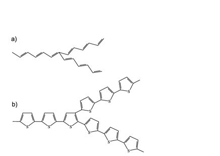
Figure 1: Sketch of branched conducting polymers.

II Steady state excitons in a star-branched polymer

Excitons in conducting polymers are the main charge carriers in photophysical processes and organic optoelectronic devices. Developing realistic models exciton migration is of crucial importance for engineering novel functional materials and optimization of existing ones. Apart from the exciton transport, description of steady state excitons allows to understand basic factors playing important role in exciton-lattice, exciton-phonon and other interactions. Different models for exciton dynamics in conjugated polymers have been proposed so far in the literature (see, e.g., Refs.Exc1 ; Exc2 ; Exc3 ; Exc4 ; Exc5 ). For conducting polymers, due to their quasi-one dimensional and periodic structure, a polymer chain can be considered as a one-dimensional lattice of monomers. Therefore, most of the models describing excitons in conducting polymers are the 1D models. This allows, e.g., to use 1D tight-binding approach, to calculate band structure and charge carrier migration. Such approach was proposed first in Rice . Here we consider dynamics of excitons in a branched conducting polymers that consist of three polymer chains, which are connected to each other at single monomer (see, Fig.1). The model we will use in this paper is close to that proposed by Abe in the Ref.Exc2 and assumes neglecting of electrons-phonon interactions, considers lattice as rigid and Coulomb interaction between the electron is assumed to be weak compared to that of between the electron and the hole. Also, to avoid appearing of the infinite binding energy, we include a cut-off length into the Coulomb potential Exc2 . Then the attractive Coulomb potential between the electron and hole can be written as

$$V(x)=-\frac{1}{|x+\xi|}.$$

Figure 2: Basic star graph.

Here we consider branched polymer in the form of Y-junction (see, Fig.1). However, our approach can be applied for arbitrary branching topology. Such system can be mapped onto the basic star graph presented in Fig.2. We assume that the size of the exciton is much smaller than that of polymer branch and both electron and hole belong to the same branch. Then the dynamics of electron-hole pair can be effectively reduced to one-particle description in terms of center-of-mass coordinates (see Appendix for details of separation of variables in the two-particle Schrödinger equation). The stationary Schrödinger equation on metric star graph describing exciton in branched polymer (on each branch of the graph presented in Fig.2 and in the units $\hbar=e=1$) can be written as

$$\left(\frac{p^{2}}{2\mu}-\frac{1}{|x+\xi_{j}|}\right)\psi_{j}(x)=E_{b}\psi_{j}(x),$$ (II.1)

where $p=-i\frac{d}{dx},$ $E_{b}$ is the binding energy for electron-hole pair, $j$ is the number of branch. Coulomb potential describes electron-hole interaction and $\mu$ is the reduced mass given by

$$\frac{1}{\mu}=\frac{1}{m_{e}}+\frac{1}{m_{h}},$$

To solve Eq.(II.1), one needs to impose the boundary conditions at the branching points (vertices) of the graph. Here we impose them as the continuity of the wave function at the branching point:

$$\psi_{1}(0)=\psi_{2}(0)=\psi_{3}(0)$$ (II.2)

and the Kirchhoff rule, which is given by

$$\sum\limits_{j=1}^{3}{\frac{d}{dx}\psi_{j}(x=0)}=0.$$ (II.3)

As the analytical solution of Eq.(II.1) is not possible, one needs to solve it numerically for the boundary conditions (II.2) and (II.3). To do this, we expand the wave function $\psi_{j}$ in terms of the complete set of eigenvalues of star graph:

$$\psi_{j}(x)=\sum c_{n}\phi_{j,n}(x),$$ (II.4)

where $\phi_{j,n}(x)$ are the eigenvalues of the unperturbed quantum star graph given by the following Schrödinger equation Keating :

$$-\frac{1}{2}\frac{d^{2}}{dx^{2}}\phi_{j}=\varepsilon\phi_{j}$$ (II.5)

with the boundary conditions

$$\phi_{1}(0)=\phi_{2}(0)=\phi_{3}(0)$$

and current conservation

$$\sum\limits_{j=1}^{3}{\frac{d}{dx}\phi_{j}(x=0)}=0,$$

and the Dirichlet boundary conditions at the branch ends given by

$$\phi_{1}(L_{1})=\phi_{2}(L_{2})=\phi_{3}(L_{3})=0.$$

Explicitly, the eigenfunctions $\phi_{j,n}$ can be written as Keating

$$\phi_{j,n}(x)=\frac{B_{n}}{\sin{(k_{n}L_{j})}}\sin{(k_{n}(L_{j}-x))},$$ (II.6)

where

$$B_{n}=\left[\sum\limits_{j}{(L_{j}+\sin{(2k_{n}L_{j})})\sin^{-2}{(k_{n}L_{j})}}/2\right]^{-1/2}.$$

Eigenvalues, $\varepsilon$ can be found from the following secular equation:

$$\sum_{j=1}^{3}\tan^{-1}\sqrt{2\varepsilon}L_{j}=0.$$

Inserting Eq.(II.4) into (II.1) and multiplying both sides to $\phi_{j,m}^{*}$ and integrating by taking into account the normalization conditions given by

$$\int\phi_{j,m}^{*}\phi_{j,n}dx=\delta_{mn},$$

the eigenvalues, $E_{n}$ can be found by diagonalizing the matrix $W_{mn}$, which is given as

$$W_{mn}=(\varepsilon_{n}\delta_{mn}+V_{mn}),$$ (II.7)

with $\delta_{mn}$ being the Kronecker symbol and

$$V_{mn}=-\sum_{j=1}^{3}\int\limits_{0}^{L_{j}}{\frac{\phi_{j,m}^{*}\phi_{j,n}}{|x+\xi_{j}|}dx}.$$

In the following numerical calculations we choose $\xi_{1}=\xi_{2}=\xi_{3}=1$. Fig.3 presents plot of the first 20 energy levels of a steady state exciton on a branched conducting polymer as a function of the parameter, $\alpha$ given by the relation $L_{j}=\alpha l_{j},\ j=1,2,3$. The plot shows that as longer the length of branch, as smaller the binding energy electron and hole in polymer.

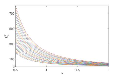
Figure 3: The first 20 energy levels of a steady state exciton on a branched conducting polymer vs the parameter $\alpha$, which is defined from the relation $L_{j}=\alpha l_{j},\ j=1,2,3.$

Important characteristics of excitons migrating in branched conducting polymers is the exciton current at each branch. The total current density is given by

$$J(x,t)=J_{1}(x,t)+J_{2}(x,t)+J_{3}(x,t),$$

where

$$J_{j}(x,t)=\frac{i}{2}\left[\Psi_{j}(x,t)\frac{\partial\Psi_{j}^{*}(x,t)}{\partial x}-\frac{\partial\Psi_{j}(x,t)}{\partial x}\Psi_{j}^{*}(x,t)\right],$$

is the current density on each branch and

$$\Psi_{j}(x,t)=\underset{n}{\sum}G_{n}e^{-ik_{n}^{2}t}\psi_{j}(x,k_{n}),$$

where coefficients $G_{n}$ are found from the initial condition for Eq.(II.1). The current can be found by integrating current density over $x$.

In Fig.4 the evolution of the current density in time and space is plotted for the initial condition given in the form of the Gaussian wave packet

$$\Psi^{I}(x)=\left(\sqrt{2\pi}\sigma_{0}\right)^{-1/2}\exp{\left(-\frac{(x-x_{0})^{2}}{4\sigma_{0}^{2}}+ip_{0}x\right)}.$$

compactly supported in the first branch and centered around $x_{0}=L_{1}/2$ with an average initial momentum $p_{0}=-5$ and width $\sigma_{0}=1$. In numerical calculations we choose lengths of the branches as $L_{1}=6.62,L_{2}=7.06$ and $L_{3}=6.36$.

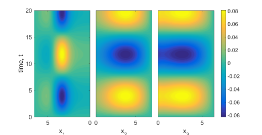
Figure 4: Spatio-temporal evolution of the current density for the initial wave packet given in the form of a Gaussian with parameters $x_{0}=L_{1}/2$, $p_{0}=-5$, $\sigma_{0}=1$. Lengths of the branches are $L_{1}=6.62,L_{2}=7.06$ and $L_{3}=6.36$.

III Transport of excitons

Important issue in modeling of exciton dynamics conducting polymers is migration of excitons along the polymer chain. In case of branched conducting polymer, dynamics become richer due to the transmission or reflection of exciton at the branching point. Here we consider this problem by modeling exciton dynamics in terms of the time-dependent Schrödinger equation on metric graph, which is given by (in the system of units $\mu=\hbar=1$)

$$i\frac{\partial\psi_{j}}{\partial t}+\frac{1}{2}\frac{d\psi_{j}}{dx^{2}}+\left(\frac{1}{x+\xi_{j}}\right)\psi_{j}=0,\,\,x\in b_{j}$$ (III.1)

where $\mu$ is the reduced mass, $\xi_{j}>0$ is the cutoff length and $j$ is the branch number. The boundary conditions are imposed as continuity of the wave function weight

$$\alpha_{1}\psi_{1}(0,t)=\alpha_{2}\psi_{2}(0,t)=\alpha_{3}\psi_{3}(0,t),$$ (III.2)

and current conservation

$$\frac{1}{\alpha_{1}}\partial_{x}\psi_{1}(x=0,t)=\frac{1}{\alpha_{2}}\partial_{x}\psi_{2}(x=0,t)+\frac{1}{\alpha_{3}}\partial_{x}\psi_{3}(x=0,t),$$ (III.3)

where $\alpha_{j},\,j=1,2,3$ are real constants. Dirichlet boundary conditions are imposed at the end of each branch:

$$\psi_{j}(x=L_{j},t)=0,\,j=1,2,3.$$ (III.4)

When these boundary conditions are applied to branched conducting polymers, $\alpha_{j}$ can be chosen as hopping constants of the polymer “lattice”, or any physical characteristic of a branch, e.g., its conductance.

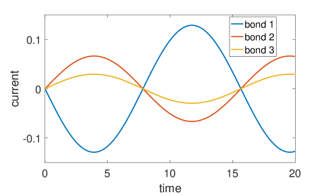
Figure 5: Time-dependence of current on each branch for the case shown in Fig. 4.

Here we use concept of so-called transparent boundary conditions (TBC) for quantum graphs, which was introduced recently in the Refs.Jambul ; Jambul02 . Unlike the scattering matrix based approach widely used in quantum mechanics, this novel approach allows to introduce reflectionless propagation of the waves in terms of boundary conditions for the wave equation. Although explicit form of these boundary conditions are very complicated and numerical solution of the problem requires using highly accurate and stable discretization scheme, application of the approach to quantum graphs allows considerable simplification. Namely, as it was shown in Jambul ; Jambul02 , under certain constraints, transparent boundary conditions become equivalent to usual continuity and Kirchhoff rules given by Eqs. (III.2) and (III.3). Therefore, the method proposed in Jambul ; Jambul02 may become powerful approach for solving the problem of reflectionless wave propagation in branched structures modeled in terms of quantum graphs.

It was shown in Jambul ; Jambul02 that the vertex boundary conditions given by Eqs.(III.2) -(III.4) become equivalent to the transparent boundary conditions, i.e., provide reflectionless transmission of the wave through the branching point, when parameters $\alpha_{j}$ fulfill the following sum rule:

$$\frac{1}{\alpha_{1}^{2}}=\frac{1}{\alpha_{2}^{2}}+\frac{1}{\alpha_{3}^{2}}$$ (III.5)

To check this, time evolution of the profile of the exciton’s wave function, initially chosen as a right traveling Gaussian wave packet

$$\psi^{I}(x)=(2\pi)^{-1/4}\exp(30ix-(x+5)^{2}/4),$$

has been simulated. The Crank-Nicolson finite difference scheme with the space discretization $\Delta x=0.0067$ and the time step $\Delta t=1\cdot 10^{-5}$ has been used in this calculations. The result of this numerical experiment is plotted in Fig. 6, for the values of BC parameters $\alpha_{1}=\sqrt{2/3}$, $\alpha_{2}=1$, $\alpha_{3}=\sqrt{2}$. Reflectionless transmission of the exciton through the polymer branching point can be seen from this plot.

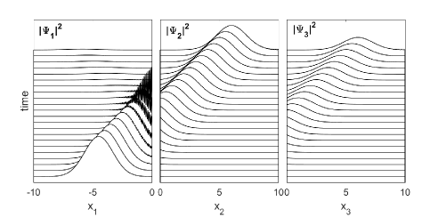
Figure 6: The profile of the exciton’s wave function on a branched conducting polymer for the values of $\alpha_{j}$ fulfilling the sum rule in Eq. (III.5): $\alpha_{1}=\sqrt{2/3}$, $\alpha_{2}=1$, $\alpha_{3}=\sqrt{2}$.

IV Conclusions

We studied steady states and migration of exciton in branched conducting polymers. A model based on the use of quantum graph concept, described by the linear Schrödinger equation on metric graphs is applied. The main focus is given to calculation of the energy spectra of steady state exciton and to the transport along the polymer chains accompanied the transmission (reflection) of exciton at the branching points. Combining the quantum graphs and transparent boundary conditions concepts, constraints providing the reflectionless transmission of exciton through the branching point is derived in the form of a simple sum rule. Numerical computations showing such transmission are provided in addition to the analytical results. The model proposed in this work can be extended to the case of more complicated branching topologies. Also, it can be applied for modeling of exciton migration in polymer based thin film organic solar cells, where polymer chains packed on the cell create complicated branched structures.

Appendix: Two particle system on a quantum graph

Remarkable feature of quantum-mechanical two particle motion is the fact that variables in the Schrödinger equation can be separated in center of mass and inter-distance variables. This allows one to reduce two-particle motion effectively to one-particle description. Here we will show that similar reducing is possible for two-particle motion on quantum graphs. Consider the star graph with three branches $b_{j}$, for which coordinates $x_{1j},\,x_{2j}$ are assigned. Choosing the origin of coordinates at the vertex, 0, for each branch $b_{j}$ we put $x_{1j},\,x_{2j}\in[0,L_{j}]$. In what follows, we use the shorthand notation $\psi_{j}(x_{1},x_{2})$ for $\psi_{j}(x_{1j},x_{2j})$, where $x_{1},\,x_{2}$ are the coordinates on the branch $j$ to which the component $\psi_{j}$ refers.

Then assuming that both particles are located in the same branch and the distance between the particles are much shorter than the length of the branch, one can write the Schrödinger equation describing such two particle system on each branch of graph, $b_{j}\sim[0;L_{j}]$ as

$$i\hbar\frac{\partial\psi_{j}}{\partial t}=-\frac{\hbar^{2}}{2m_{1}}\frac{\partial^{2}\psi_{j}}{\partial x_{1}^{2}}-\frac{\hbar^{2}}{2m_{2}}\frac{\partial^{2}\psi_{j}}{\partial x_{2}^{2}}+U_{j}(x_{1}-x_{2})\psi_{j},$$ (IV.1)

where $U_{j}(x_{1}-x_{2})$ is the potential of interaction between the particles. Furthermore, we introduce the relative coordinate $x=x_{1}-x_{2}$ and the center-of-mass coordinate $X=\frac{m_{1}x_{1}+m_{2}x_{2}}{m_{1}+m_{2}}$. In terms of these new coordinates, $x$ and $X$ in Eq. (IV.1) can be rewritten as

$$i\hbar\frac{\partial\psi_{j}}{\partial t}=-\frac{\hbar^{2}}{2\mu}\frac{\partial^{2}\psi_{j}}{\partial x^{2}}-\frac{\hbar^{2}}{2(m_{1}+m_{2})}\frac{\partial^{2}\psi_{j}}{\partial X^{2}}+U_{j}(x)\psi_{j},$$ (IV.2)

where $\mu=\frac{m_{1}m_{2}}{m_{1}+m_{2}}$. Separating variables in Eq.(IV.2) and using the substitution

$$\psi_{j}(x,X,t)=\psi_{jM}(X)\psi_{j\mu}(x)e^{-i\hbar Et},$$ (IV.3)

we get

$$-\frac{\hbar^{2}}{2\mu}\frac{\partial^{2}\psi_{j\mu}}{\partial x^{2}}+U_{j}(x)\psi_{j\mu}=E_{b}\psi_{j\mu},$$

$$\frac{\hbar^{2}}{2(m_{1}+m_{2})}\frac{\partial^{2}\psi_{jM}}{\partial X^{2}}+\hbar^{2}E\psi_{jM}=E_{b}\psi_{jM}.$$ (IV.4)

Thus center of mass and relative (inter-distance) motions can be separated when electron and hole belong in the same branch. However, this does not automatically apply to the case of transmission of exciton through the branching area. In that case, depending on the distance between electron and hole, they may appear in different branches. Therefore, to avoid such a situation and provide separation of variables in such case, one needs to make additional assumptions. Here we assume that the size of the branching area is comparable or larger that that of exciton.

- (1) R.J. Kline, M.D. McGehee, J. Macromolecular Sci. C, 46 27 (2006).
- (2) D.S. Wallacet A.M. Stonehams, W. Hayest, A.J. Fishertt and A. Testas, J. Phys.: Condens. Matter 3 3905 (1991).
- (3) D. Kumar, R. C. Sharma, Eur. Polym. J., 34 1053 (1998).
- (4) W.R. Salaneck, R.H. Friend, J.L. BreHdas, Phys. Rep., 319 231 (1999).
- (5) A.J. Heeger and R. Pethig, Phil. Trans. R. Soc. Lond. A 314 17 (1985).
- (6) A.J. Heeger, Rev. Mod.Phys. 73 681 (2001).
- (7) A.J. Heeger, S. Kivelson, J.R. Schrieffer, W.-P. Su, Rev. Mod.Phys. 60 781 (1988).
- (8) K. Maki, Synth. Met., 9 185 (1984).
- (9) L. Rothberg, T. M. Jedju, S. Etemad, G. L. Baker, Phys. Rev. Lett. 57 3229 (1982).
- (10) M. Kuwabara, S. Abe, and Y. Ono, Synth. Met., 85 1109 (1997).
- (11) P.B. Miranda, D. Moses, A.J. Heeger, Y.W. Park, Phys. Rev. B, 66 125202 (2002).
- (12) A.J. Heeger, S. Kivelson, J.R. Schrieffer, W.-P. Su, Rev. Mod.Phys. 60 781 (1988).
- (13) S. Brazovskii, Solid State Sci. 10 1786 (2008).
- (14) W.P. Su, Schrieffer, A.J. Heeger, Phys. Rev. Lett., 42 1698 (1979).
- (15) L. Bernasconi, J.Phys. Chem. Lett., 6 908 (2015).
- (16) M. Sasai, H. Fukutome, Prog. Theor. Phys., 79 61 (1988).
- (17) S. Suhai, J. Chem. Phys., 73 3843 (1980).
- (18) M.J. Rice, Yu.N. Gartstein, Phys. Rev. Lett. 73 2504 (1994).
- (19) S. Brazovskii, N. Kirova, A.R. Bishop, Opt. Mat., 9 465 (1998).
- (20) D. Moses, J. Wang, A.J. Heeger, N. Kirova, S. Brazovski, Synth. Met., 119 503 (2001).
- (21) N. Kirova, S. Brazovskii, Thin Solid Films, 403 419 (2002).
- (22) N. Kirova, S. Brazovskii, Synth. Met., 141 139 (2004).
- (23) N. Kirova, S. Brazovskii, Current Appl. Phys., 4 473 (2004).
- (24) M. N. Kobrak, E. R. Bittner, J. Chem. Phys., 112 5399 (2000).
- (25) H. Tamura, E.R. Bittner, I. Burghardt, J. Chem. Phys. 126,021103 (2007).
- (26) H. Tamura, J.G.S. Ramon, E.R. Bittner, I. Burghardt, Phys. Rev. Lett. B 100, 107402 (2008).
- (27) W. Barford, E.R. Bittner, A. Ward, J. Phys. Chem. 116, 10319 (2012).
- (28) M. Fujii, K. Ari and K. Yoshino, J. Electrochem. Soc., 140 7, (1993).
- (29) J. Jurkiewicz and A. Krzywicki Phys. Lett. B 392, 29 (1997).
- (30) K. Inoue, Prog. Polym. Sci. 25, 453 (2000).
- (31) L. Dai, B. Winkler, L. Dong, L. Tong and A. W. H. Mau, Adv. Mater., 13, 12-13 (2001).
- (32) D. T. Wu, Synth. Met., 126, 289 (2002).
- (33) C. Gao and D. Yan Prog, Polym. Sci. 29, 183 (2004).
- (34) F. Hua and E. Ruckenstein, Macromolecules 38, 888 (2005).
- (35) R.-H. Lee, W.-Sh. Chen, and Y.-Y. Wang, Thin Solid Films, 517, 5747 (2009)
- (36) A. Hirao and H.-S. Yoo, Polymer Journal, 43, 2 (2011).
- (37) L. R. Hutchings Macromolecules, 45, 5621 (2012).
- (38) J. Ohshita, Y. Tominaga, D. Tanaka, T. Mizumo, Y. Fujita, Y. Kunugi, J. Org. Chem., 50, 736 (2013).
- (39) G. V. Otrokhov, O. V. Morozova, I. S. Vasileva, G. P. Shumakovich, E. A. Zaitseva, M. E. Khlupova, and A. I. Yaropolov, Biochemistry, 78, 1539 (2013).
- (40) M. Goll, A. Ruff, E. Muks, F. Goerigk, B. Omiecienski, I. Ruff, R. C. Gonzalez-Cano, J. T. L. Navarrete, M. C. R. Delgado and S. Ludwigs, Beilstein J. Org. Chem., 11, 335 (2015).
- (41) H Higginbotham, K. Karon, P. Ledwon and Display and Przemyslaw Data, Imaging, 2, 207 (2017).
- (42) T. Soganci, O. Gumusay, H. C. Soyleyici , M. Ak, Polymer 134, 187 (2018).
- (43) Ch. Wu, S.V. Malinin, S. Tretiak, V.Y. Chernyak, Nature Physics, 2, 631635 (2006).
- (44) Ch. Wu, S.V. Malinin, S. Tretiak, and V.Y. Chernyak, J. Chem. Phys., 129, 174111 (2008).
- (45) Ch. Wu, S.V. Malinin, S. Tretiak, and V.Y. Chernyak, J. Chem. Phys., 129, 174112 (2008).
- (46) Ch. Wu, S.V. Malinin, S. Tretiak, and V.Y. Chernyak, J. Chem. Phys., 129, 174113 (2008).
- (47) H. Li, S.V. Malinin, S. Tretiak, and V.Y. Chernyak, J. Chem. Phys., 132, 124103 (2010).
- (48) H. Li, Ch. Wu, S.V. Malinin, S. Tretiak, V.Y. Chernyak, J. Phys. Chem. B, 115(18), pp.5465-5475 (2011).
- (49) H. Li, S.V. Malinin, S. Tretiak, and V.Y. Chernyak, J. Chem. Phys., 139, 064109 (2013).
- (50) H. Li, M.J. Catanzaro, S. Tretiak, V.Y. Chernyak, J. Phys. Chem. Lett., 5(4), pp.641-647 (2014).
- (51) V.Kostrykin and R.Schrader J. Phys. A: Math. Gen. 32 595 (1999)
- (52) T.Kottos and U.Smilansky, Ann.Phys., 76 274 (1999).
- (53) P.Kuchment, Waves in Random Media, 14 S107 (2004).
- (54) S.Gnutzmann and U.Smilansky, Adv.Phys. 55 527 (2006).
- (55) P.Exner and H.Kovarik, Quantum waveguides. (Springer, 2015).
- (56) J.P.Keating, Contemp. Math., 415, 191 (2006).
- (57) S.Gnutzmann, J.P.Keating, F. Piotet, Ann.Phys., 325 2595 (2010).
- (58) K.K.Sabirov, J.Yusupov, D. Jumanazarov, D. Matrasulov, Phys.Lett. A, 382, 2856 (2018).
- (59) D.U. Matrasulov, J.R. Yusupov and K.K. Sabirov, J. Phys. A, 52, 155302 (2019).
- (60) J.R. Yusupov, K.K. Sabirov, M. Ehrhardt and D.U. Matrasulov, Phys. Lett. A, 383, 2382 (2019).
- (61) Aripov M.M., Sabirov K.K., Yusupov J.R., Nanosystems: physics, chemistry, mathematics, 10(5), P.501-602 (2019).
- (62) J.R. Yusupov, K.K. Sabirov, M. Ehrhardt and D.U. Matrasulov, Phys. Rev. E, 100, 032204 (2019).
- (63) D. Babajanov, H. Matyoqubov and D. Matrasulov, J. Chem. Phys., 149, 164908 (2018).
- (64) Th G. Pedersen, Phys. Rev. B 69 075207 (2004).
- (65) Sh. Abe, J. Phys. Soc. Jpn. 58 62 (1989).
- (66) Sh. Abe, et.el. Phys. Rev. B 45 9432 (1992).
- (67) Sh. Abe, J. Yu, W. P. Su, Phys. Rev. B 45 8264 (1992).
- (68) A. V. Nenashev, Phys. Rev. B 84 035210 (2011).