Electromagnetic properties of the nucleon and the Roper resonance
in soft-wall AdS/QCD at finite temperature

Abstract

We present a study of the nucleon electromagnetic form factors and of the Roper-nucleon transition at finite small temperature $T$, using an extended version of a soft-wall AdS/QCD approach developed by us previously. In the action we introduce the effective potential, which has quadratic dependence on the holographic coordinate $z$ and depends on both the gluon and quark condensates. Choosing the AdS geometry we restrict ourselves to the AdS Poincaré metric, because the contribution of the AdS-Schwarzschild geometry starts at next-to-leading order ${\cal O}(T^{4})$. Hence, one can neglect the temperature dependence of the AdS geometry at small $T$. This is consistent with the Hawking-Page phase transition at a critical temperature representing the transition between thermal AdS/QCD and AdS-Schwarzschild geometry. In the small temperature regime we base our analysis on the temperature dependence of the effective potential, which starts at order ${\cal O}(T^{2})$, due to the leading contribution from the quark condensate. As applications we present the analysis of properties of the nucleon and Roper resonance (masses, form factors, and helicity amplitudes) at low temperatures.

1 Introduction

The study of baryons in the soft-wall AdS/QCD approach was first laid out in Refs. [1, 2], where an effective action was proposed, describing the nucleon confining dynamics and the minimal (nonminimal) couplings to the electromagnetic field. Based on this action the electromagnetic form factors of the nucleon were calculated, and later, in Refs. [3]-[18], the soft-wall AdS/QCD approach in the baryon sector was modified/improved in different directions. It was applied to the calculation of generalized parton distributions of the nucleon [3], extended to account for higher Fock states in the nucleon and to additional couplings with the electromagnetic field [4]. This last extension leads to consistency with QCD constituent counting rules [5] for the power scaling of hadronic form factors at large values of the Euclidean momentum transfer squared. In Ref. [6] the soft-wall AdS/QCD approach was further developed to describe baryons with adjustable quantum numbers $n$, $J$, $L$, and $S$. In another development, in Refs. [7, 8], the nucleon properties were analyzed using a Hamiltonian formalism. In Ref. [9] a version of the soft-wall AdS/QCD approach was proposed, where a modified warp factor in the metric tensor is present. Note that in Ref. [6] we proved that any modification of the warp factor in the metric tensor can be compensated by an appropriate choice of the holographic potential. The form of such potentials for AdS fields with different spins were also derived analytically.

The soft-wall AdS/QCD formalism is also useful for constraining other approaches. In particular, in Refs. [10, 11] we developed a light-front quark-diquark approach to nucleon structure describing nucleon parton distributions and form factors from a unified point of view. In particular, in Ref. [11] we derived nucleon light-front wave functions, analytically matching the results of global fits to the quark parton distributions in the nucleon at the initial scale $\mu\sim 1$ GeV. We also showed that these distributions obey the correct Dokshitzer-Gribov-Lipatov-Altarelli-Parisi evolution [12] up to high scales. Using these constraints for the nucleon wave functions, we got a reasonable description of data of the nucleon electromagnetic form factors. We also made predictions for other nucleon quark distributions (transverse momentum, Wigner and Husimi distributions) from a unified point of view, using our light-front wave functions and expressing them in terms of the parton distributions $q_{v}(x)$ and $\delta q_{v}(x)$.

Nucleon resonances have also been discussed in the AdS soft-wall approach in Refs. [13]-[16]. In Ref. [13] the Dirac form factor for the electromagnetic nucleon-Roper transition was calculated in light-front holographic QCD. Later, in Ref. [14], a formalism for the study of all nucleon resonances in soft-wall AdS/QCD has been proposed. As a first application, a detailed description of Roper-nucleon transition properties (form factors, helicity amplitudes and transition charge radii) was performed. In Ref. [16] we presented an improved study of the electromagnetic form factors of the nucleon and of the Roper, using an extended version of the effective action of soft-wall AdS/QCD. At this point additional non-minimal terms were included, which do not renormalize the charge and give an important contribution to the momentum dependence of the form factors and helicity amplitudes.

The study of hadron properties at finite temperature gives a unique opportunity for the understanding of the evolution of the early Universe after the Big Bang. It also permits to investigate physical principles related to the formation of hadronic matter and its phase transitions (confinement and deconfinement, chiral symmetry restoration). From experiments, e.g., on quark-gluon plasma formation, we know that hadron properties change under the influence of in-medium effects (density and temperature). Therefore, the investigation of the temperature behavior of hadrons is a worthwhile task to pursue. One of the most interesting hadronic characteristics to study is the temperature dependence of masses and form factors. In Refs. [17, 18] we derived a soft-wall AdS-Schwarzschild approach at small temperatures, in which we included temperature dependence due to the propagation of AdS fields in the AdS-Schwarzchild metric and due to the explicit $T$ dependence of the dilaton scale parameter $\kappa$. We performed a temperature expansion of hadronic quantities in the form of an $T^{2}/(12F^{2})$ expansion dictated by QCD [19]-[21] and noticed that the AdS-Schwarzschild thermal factor $f_{T}(z)=1-(\pi Tz)^{4}$ gives a contribution at next-to-leading order, i.e. at order ${\cal O}(T^{4})$, while the $T$ dependence of the dilaton shows up already at leading order ${\cal O}(T^{2})$. Our approach was applied to the description of hadrons with integer and half-integer spin and adjustable number of constituents (mesons, baryons, tetraquarks, etc.) with analytical results for the temperature dependence of their masses and form factors. Note that originally the idea of a thermal dilaton — dilaton field depending on temperature was proposed in Ref. [22]. Two thermal dilaton forms were studied resulting in melting temperatures for mesons close to 180 MeV.

In the present paper, using our findings of Refs. [17, 18], we present a more detailed discussion of the effective holographic potential providing spontaneous breaking of conformal and chiral symmetry and generating a temperature dependence. Using the fact that the holographic potential has leading ${\cal O}(T^{2})$ we restrict to the use of the pure AdS Poincaré metric, which is more relevant in small temperature regime in comparison with the AdS-Schwarzchild geometry, which is more suitable at high $T$.

The paper is organized as follows. In Sec. II we briefly discuss our formalism. In Sec. III we present the analytical calculation and the numerical analysis of electromagnetic form factors and helicity amplitudes of the nucleon and the Roper at finite temperature. Finally, Sec. IV contains our summary and conclusions.

2 Formalism

In this section we briefly review our approach [16]. We start with the definition of the conformal Poincaré metric

$$g_{MN}\,x^{M}x^{N}=\epsilon^{a}_{M}\,\epsilon^{b}_{N}\,\eta_{ab}\,x^{M}x^{N}=\frac{1}{z^{2}}\,(dx_{\mu}dx^{\mu}-dz^{2})$$ (1)

where $\epsilon^{a}_{M}=\delta^{a}_{M}/z$ is the vielbein, and we define $g=|{\det}(g_{MN})|=1/z^{10}$ as the magnitude of the determinant of $g_{MN}$.

The soft-wall AdS/QCD action $S$ for the nucleon $N=(p,n)$ and the Roper ${\cal R}=({\cal R}_{p},{\cal R}_{n})$ resonance, including photons, is constructed in terms of the dual spin-$1/2$ fermion and vector fields. They have constrained (confined) dynamics in AdS space due to the presence of a quadratic ($z^{2}$) holographic potential. One can derive such a potential in the action: (1) via an exponential prefactor containing the background field or (2) directly as an interaction potential. We proved in Ref. [6] that both versions of the soft-wall AdS/QCD model are equivalent to each other. As was first shown in Ref. [1] and later confirmed in Ref. [2], in the case of baryons the exponential prefactor can be simply removed after proper redefinition of the AdS fermion fields, which means that the direct inclusion of the holographic potential is essential. Such a potential was constructed for the first time in Refs. [1, 2]: $U_{F}(z)=\varphi(z)=\kappa^{2}z^{2}$, where $\varphi$ is the quadratic dilaton field and $\kappa$ is its size parameter. Keeping in mind that the most fundamental property of baryons is their mass. It can be expressed in terms of vacuum condensates using methods of QCD sum rules [23, 24], where at leading order the nucleon mass is related to the quark condensate (so-called Ioffe formula) [23] by:

$$M_{N}^{3}\simeq 8\,\pi^{2}\,\Sigma\,,$$ (2)

where $\Sigma=|\langle 0|\bar{q}q|0\rangle|$ is the quark condensate. The Ioffe formula gives reasonable agreement with data. However, as stressed in Ref. [25], there is a puzzle, since this formula implies that a large contribution to baryon masses comes from the quark condensate. In the overview to this problem presented in Ref. [25] it is mentioned that conceptually different theoretical approaches (lattice QCD [26], chiral quark-soliton model [27], dilaton compensated model based on hidden local symmetry [28], holographic QCD [29]) arrived at similar conclusions, which is that the main source of the baryon mass is due to the quark condensate independent term $m_{0}$ plus a correction due to the quark condensate. In particular, in Ref. [28] the following formula for the baryon mass $M_{B}$ was proposed:

$$M_{B}=m_{0}+\Delta(\Sigma)\,,$$ (3)

where $\Delta(\Sigma)$ is the correction due to the quark condensate. In Ref. [29] it was found that there are two different regimes of low and large values of the quark condensate $\Sigma=(N_{c}/2\pi^{2})\,\sigma$. At low values of $\sigma$ the baryon mass is saturated by the condensate independent term $887$ MeV controlled by the confinement scale, while at large values of $\sigma$ it is defined by the scalar repulsion force and linearly depends on the quark condensate [29]:

$$M_{B}={\rm max}[887;-407+940\,(z_{m}\sigma^{1/3})]\ {\rm MeV}\,,$$ (4)

where $z_{m}=(323\ {\rm MeV})^{-1}$ is the position of the infrared hard wall in the holographic approach that we are considering. Note that the physical explanation of the dominant term $m_{0}$ is different in various approaches: constituent quark mass, qluon condensate, skyrmion, etc.

In our approach the baryon masses are proportional to the scale parameter $\kappa$ occurring in the $z^{2}$ dependent holographic potential $U_{F}(z)=\kappa^{2}z^{2}$. This corresponds to the square of the linearized part of the Cornell potential, because the equation of motion (EOM) for the wave function with $U_{F}$ corresponds to the square of the EOM with the Cornell potential, as proven in Refs. [30, 31]. Here $\kappa=383$ MeV is the dilaton scale parameter fixed in the previous study. In order to get explicit expressions for the baryon masses in terms of quark condensates we parametrize the scale parameter as:

$$\kappa^{2}=\kappa^{2}\,(1-y)\,+\,\frac{\pi^{2}\,\Sigma}{M_{N}}\,y\,,$$ (5)

where $y$ is the mixing parameter. The specific normalization of the condensate containing term is chosen for convenience. The squared nucleon mass in the soft-wall AdS/QCD model, for leading twist $\tau=3$, is given by [6]:

$$M_{N}^{2}=8\,\kappa^{2}\,,$$ (6)

then one gets:

$$M_{N}^{2}=8\,\kappa^{2}\,(1-y)\,+\,\frac{8\,\pi^{2}\,\Sigma}{M_{N}}\,y\,.$$ (7)

Next, using the Ioffe formula (2) one has

$$M_{N}^{2}=8\,\kappa^{2}\,(1-y)\,+\,M_{N}^{2}\,y\,.$$ (8)

This last relation has a very clear physical meaning. Here and in Eq. (5) the limits $y=0$ and $y=1$ correspond to the cases of vanishing and fully dominating quark condensates in the expression for the nucleon mass and $\kappa^{2}$. In previous papers we consider the case $y=1$. Here we vary the parameter $y$ and investigate the dependence on $y$ of the nucleon and Roper resonance properties, and we do not specify the physical content of the parameter $\kappa^{2}$, which might be a combination of gluon condensates of dimension 2 and 4. It is important that these gluon condensates have a suppressed temperature dependence at small $T$ in comparison with the quark condensate. In particular, the temperature dependence of the dimension-2 gluon condensate ${\cal O}_{A^{2}}=\langle A_{\mu}^{2}\rangle$ has been analyzed in a formalism of local composite operators [32], where tt was shown that no ${\cal O}(T^{4})$ temperature corrections arise for this condensate at small $T$. The study of the temperature dependence of the dimension-4 gluon condensate ${\cal O}_{G^{2}}=\langle{\rm tr}\,G_{\mu\nu}^{2}\rangle$ has been initiated by Leutwyler in Ref. [33] and later it was extensively studied, e.g., in $SU(2)$ and $SU(3)$ lattice gauge theories in Ref. [34]. There it was shown that in both cases the temperature corrections start at order ${\cal O}(T^{4})$, but are small numerically, making the condensate to be constant for small $T<T_{c}$, where $T_{c}=290$ MeV for $SU(2)$ and $264$ MeV for $SU(3)$. Therefore, the main source of the temperature dependence of the holographic potential in the low $T$-region comes from the quark condensate. The temperature dependence of the holographic potential will disappear when $\Sigma$ vanishes which corresponds to the restoration of spontaneously broken chiral symmetry. In QCD the quark condensate depends on temperature and vanishes at the critical temperature $T_{c}$, which signals the restoration of chiral symmetry. Such temperature dependence of the quark condensate up to $T_{c}$, was calculated by Gasser, Leutwyler, and Gerber using chiral perturbation theory (ChPT) [19, 20] in the form of an $T^{2}/(12F^{2})$ expansion dictated by QCD at two [19] and three loops [20]. In particular, the result for two-loop ChPT reads:

$$\Sigma(T) = \Sigma\ \sigma(T)\,,$$

$$\sigma(T) = 1+\delta_{T_{1}}\frac{T^{2}}{12F^{2}}\,+\,\delta_{T_{2}}\biggl{(}\frac{T^{2}}{12F^{2}}\biggr{)}^{2}\,+\,{\cal O}(T^{6})\,,$$

$$\delta_{T_{1}} = -\frac{N_{f}^{2}-1}{N_{f}}\,,\quad\delta_{T_{2}}\,=\,-\frac{N_{f}^{2}-1}{2N_{f}^{2}}\,,$$ (9)

where $F$ is the pseudoscalar coupling constant in the chiral limit, and $N_{f}$ is the number of quark flavors. Note that the quark condensate has an entirely non-perturbative origin, while its $T$-dependence has been calculated in an expansion in powers of $T^{2}/(12F^{2})$ using ChPT. The thermal quark condensate is normalized at zero temperature as $\Sigma(0)=\Sigma$, while it vanishes $\Sigma(T_{c})=0$ at the critical temperature $T_{c}$, i.e. at the temperature when the sponeously broken chiral symmetry is restored. Therefore, the temperature dependence of the holographic potential $U_{F}(z)$ can be fixed by the temperature dependence of the quark condensate, which has been evaluated using ChPT:

$$U_{F}(z,T)=\kappa^{2}(T)\,z^{2}\,,$$ (10)

where $\kappa^{2}(T)$ is the temperature dependent scale parameter:

$$\kappa^{2}(T)=\kappa^{2}\,(1-y)\,+\,\frac{\pi^{2}\,\Sigma(T)}{M_{N}}\,y\,.$$ (11)

Using the relations derived above one can rewrite $\kappa^{2}(T)$ in a more convenient form

$$\kappa^{2}(T)=\kappa^{2}\bigg{(}1+y\,\Big{[}\sigma(T)-1\Big{]}\biggr{)}\,.$$ (12)

In our numerical analysis we present results for the quark condensate below the critical temperature $T_{c}$, which is fixed from the condition $\sigma(T_{c})=0$. Using Eq. (2) we have

$$\frac{T_{c}^{2}}{12F^{2}}=N_{f}\,\biggl{[}\sqrt{\frac{N_{f}^{2}+1}{N_{f}^{2}-1}}-1\biggr{]}\,.$$ (13)

For the case in which the number of quark flavors is set to $N_{f}=2$ one gets $T_{c}=179$ MeV. Therefore, the study of the $T$-dependence of baryon properties provides a good possibility to check the contribution of the quark condensate to their observables, e.g., masses and form factors.

Now let us specify the action relevant for the study of properties of the nucleon and Roper resonance. The action $S$ contains a free part $S_{0}$, describing the confined dynamics of AdS fields, and an interaction part $S_{\rm int}$, describing the interactions of fermions with the vector field

$$S = S_{0}+S_{\rm int}\,,$$

$$S_{0} = \int d^{4}xdz\,\sqrt{g}\,e^{-\varphi(z,T)}\,\biggl{\{}{\cal L}_{N}(x,z,T)+{\cal L}_{\cal R}(x,z,T)+{\cal L}_{V}(x,z,T)\biggr{\}}\,,$$

$$S_{\rm int} = \int d^{4}xdz\,\sqrt{g}\,e^{-\varphi(z,T)}\,\biggl{\{}{\cal L}_{VNN}(x,z)+{\cal L}_{V{\cal R}{\cal R}}(x,z,T)+{\cal L}_{V{\cal R}N}(x,z,T)\biggr{\}}\,.$$ (14)

where ${\cal L}_{N}$, ${\cal L}_{\cal R}$, ${\cal L}_{V}$ and ${\cal L}_{VNN}$, ${\cal L}_{V{\cal RR}}$, ${\cal L}_{V{\cal R}N}$ are the free and interaction Lagrangians, respectively, which are written as

$${\cal L}_{B}(x,z,T) = \sum\limits_{i=+,-;\,\tau}\,c_{\tau}^{B}\,\bar{\psi}^{B}_{i,\tau}(x,z,T)\,\hat{\cal D}_{i}(z)\,\psi^{B}_{i,\tau}(x,z,T)\,,$$

$${\cal L}_{V}(x,z,T) = -\frac{1}{4}V_{MN}(x,z,T)V^{MN}(x,z,T)\,,$$

$${\cal L}_{VBB}(x,z,T) = \sum\limits_{i=+,-;\tau}\,c_{\tau}^{B}\,\bar{\psi}^{B}_{i,\tau}(x,z,T)\,\hat{\cal V}^{B}_{i}(x,z,T)\,\psi^{B}_{i,\tau}(x,z,T)\,,$$

$${\cal L}_{V{\cal R}N}(x,z,T) = \sum\limits_{i=+,-;\,\tau}\,c_{\tau}^{{\cal R}N}\,\bar{\psi}_{i,\tau}^{\cal R}(x,z,T)\,\hat{\cal V}^{{\cal R}N}_{i}(x,z,T)\,\psi_{i,\tau}^{N}(x,z,T)\,+\,{\rm H.c.}\,,$$ (15)

where $B=N,{\cal R}$ and

$$\hat{\cal D}_{\pm}(z,T) = \frac{i}{2}\Gamma^{M}\!\stackrel{{\scriptstyle\leftrightarrow}}{{\partial}}_{{}_{M}}-\frac{i}{8}\Gamma^{M}\omega_{M}^{ab}[\Gamma_{a},\Gamma_{b}]\,\mp\,(\mu+U_{F}(z,T))\,,$$

$$\hat{\cal V}^{H}_{\pm}(x,z,T) = Q\,\Gamma^{M}V_{M}(x,z,T)\,\pm\,\frac{i}{4}\,\eta_{V}^{H}\,[\Gamma^{M},\Gamma^{N}]\,V_{MN}(x,z,T)\,\pm\,\frac{i}{4}\,\lambda_{V}^{H}\,z^{2}\,[\Gamma^{M},\Gamma^{N}]\,\partial^{K}\partial_{K}V_{MN}(x,z,T)$$ (16)

$$\pm \,g_{V}^{H}\,\Gamma^{M}\,i\Gamma^{z}\,V_{M}(x,z,T)+\zeta_{V}^{H}\,z\,\Gamma^{M}\,\partial^{N}V_{MN}(x,z,T)\,\pm\,\xi_{V}^{H}\,z\,\Gamma^{M}\,i\Gamma^{z}\,\partial^{N}V_{MN}(x,z,T)\,.$$

Here $H=N,{\cal R},{\cal R}N$, $\mu$ is the five-dimensional mass of the spin-$\frac{1}{2}$ AdS fermion, $\mu=3/2+L$, with $L$ being the orbital angular momentum; $U_{F}(z,T)=\varphi(z,T)$ is the dilaton potential; $Q={\rm diag}(1,0)$ is the nucleon (Roper) charge matrix; $V_{MN}=\partial_{M}V_{N}-\partial_{N}V_{M}$ is the stress tensor for the vector field; $\omega_{M}^{ab}=(\delta^{a}_{M}\delta^{b}_{z}-\delta^{b}_{M}\delta^{a}_{z})/z$ is the spin connection term; and $\sigma^{MN}=[\Gamma^{M},\Gamma^{N}]$ is the commutator of the Dirac matrices in AdS space, which are defined as $\Gamma^{M}=\epsilon^{M}_{a}\Gamma^{a}$ and $\Gamma^{a}=(\gamma^{\mu},-i\gamma^{5})$.

The action (2) is constructed in terms of the 5D AdS fermion fields $\psi^{N}_{\pm,\tau}(x,z,T)$, $\psi^{\cal R}_{\pm,\tau}(x,z,T)$, and the vector field $V_{M}(x,z,T)$. Fermion fields are duals to the left- and right-handed chiral doublets of nucleons and Roper resonance ${\cal O}^{L}=(B_{1}^{L},B_{2}^{L})^{T}$ and ${\cal O}^{R}=(B_{1}^{R},B_{2}^{R})^{T}$, with $B_{1}=p,{\cal R}_{p}$ and $B_{2}=n,{\cal R}_{n}$. These fields are in the fundamental representations of the chiral $SU_{L}(2)$ and $SU_{R}(2)$ subgroups and are holographic analogues of the nucleon $N$ and Roper resonance ${\cal R}$, respectively.

The 5D AdS fields $\psi^{B}_{\pm,\tau}(x,z,T)$ are products of the left/right 4D spinor fields

$$\psi^{L/R}_{n=0,1}(x,T)=\frac{1\mp\gamma^{5}}{2}\,\psi_{n=0,1}(x,T)\,,$$ (17)

with spin $1/2$ and bulk profiles

$$F^{L/R}_{\tau,n=0,1}(z,T)=z^{2}\,f^{L/R}_{\tau,n=0,1}(z,T),$$ (18)

with twist $\tau$ depending on the holographic (scale) variable $z$:

$$\psi^{N}_{\pm,\tau}(x,z,T) = \frac{1}{\sqrt{2}}\,\left[\pm\psi^{L}_{0}(x,T)\ F^{L/R}_{\tau,0}(z,T)+\psi^{R}_{0}(x,T)\ F^{R/L}_{\tau,0}(z,T)\right]\,,$$

$$\psi^{\cal R}_{\pm,\tau}(x,z,T) = \frac{1}{\sqrt{2}}\,\left[\pm\psi^{L}_{1}(x,T)\ F^{L/R}_{\tau,1}(z,T)+\psi^{R}_{1}(x,T)\ F^{R/L}_{\tau,1}(z,T)\right]\,,$$ (19)

where

$$f^{L}_{\tau,0}(z,T) = \sqrt{\frac{2}{\Gamma(\tau)}}\,\kappa^{\tau}(T)\,z^{\tau-1/2}\,e^{-\kappa^{2}(T)z^{2}/2}\,,$$

$$f^{R}_{\tau,0}(z,T) = \sqrt{\frac{2}{\Gamma(\tau-1)}}\,\kappa^{\tau-1}(T)\,z^{\tau-3/2}\,e^{-\kappa^{2}(T)z^{2}/2}\,,$$

$$f^{L}_{\tau,1}(z,T) = \sqrt{\frac{2}{\Gamma(\tau+1)}}\,\kappa^{\tau}(T)\,z^{\tau-1/2}\,(\tau-\kappa^{2}(T)z^{2})\,e^{-\kappa^{2}(T)z^{2}/2}\,,$$

$$f^{R}_{\tau,1}(z,T) = \sqrt{\frac{2}{\Gamma(\tau)}}\,\kappa^{\tau-1}(T)\,z^{\tau-3/2}\,(\tau-1-\kappa^{2}(T)z^{2})\,e^{-\kappa^{2}(T)z^{2}/2}\,.$$ (20)

The nucleon is identified as the ground state with $n=0$ and the Roper resonance as the first radially excited state with $n=1$. In the case of the vector field we work in the axial gauge $V_{z}=0$ and perform a Fourier transformation of the vector field $V_{\mu}(x,z,T)$ with respect to the Minkowski coordinate

$$V_{\mu}(x,z,T)=\int\frac{d^{4}q}{(2\pi)^{4}}e^{iqx}V_{\mu}(q)V(q,z,T)\,.$$ (21)

We derive an EOM for the vector bulk-to-boundary propagator $V(q,z)$, dual to the $q^{2}$-dependent electromagnetic current

$$\partial_{z}\biggl{(}\frac{e^{-\varphi(z,T)}}{z}\,\partial_{z}V(q,z,T)\biggr{)}+q^{2}\frac{e^{-\varphi(z,T)}}{z}\,V(q,z,T)=0\,.$$ (22)

The solution of this equation in terms of the gamma $\Gamma(n)$ and Tricomi $U(a,b,z)$ functions reads

$$V(q,z,T)=\Gamma\Big{(}1-\frac{q^{2}}{4\kappa^{2}(T)}\Big{)}\,U\Big{(}-\frac{q^{2}}{4\kappa^{2}(T)},0,\kappa^{2}(T)z^{2}\Big{)}\,.$$ (23)

In the Euclidean region ($Q^{2}=-q^{2}>0$) it is convenient to use the integral representation for $V(Q,z,T)$ [35]

$$V(Q,z,T)=\kappa^{2}(T)z^{2}\int_{0}^{1}\frac{dx}{(1-x)^{2}}\,x^{a_{T}}\,e^{-\kappa^{2}(T)z^{2}\frac{x}{1-x}}\,,$$ (24)

where $x$ is the light-cone momentum fraction and $a_{T}=Q^{2}/(4\kappa^{2}(T))$.

The set of parameters $c_{\tau}^{N}$, $c_{\tau}^{{\cal R}}$, and $c_{\tau}^{{\cal R}N}$ induce mixing of the contribution of AdS fields with different twist dimensions. In Refs. [4, 14] we showed that the parameters $c_{\tau}^{B}$ are constrained by the condition $\sum_{\tau}\,c_{\tau}^{B}=1$, in order to get the correct normalization of the kinetic term $\bar{\psi}_{n}(x)i\!\not\!\partial\psi_{n}(x)$ of the four-dimensional spinor field. This condition is also consistent with electromagnetic gauge invariance.

The couplings $G_{V}^{H}={\rm diag}(G_{V}^{H_{1}},G_{V}^{H_{2}})$, where $G=\eta,\lambda,g,\zeta,\xi$, $\ H_{1}=p,{\cal R}_{p},{\cal R}_{p}p$ and $\ H_{2}=n,{\cal R}_{n},{\cal R}_{n}n$ are fixed from the magnetic moments, slopes, and form factors of both the nucleon and Roper, while the couplings $c_{\tau}^{{\cal R}N}$ are fixed from the normalization of the Roper-nucleon helicity amplitudes. The terms proportional to the couplings $\lambda_{V}^{H}$, $\zeta_{V}^{H}$, and $\xi_{V}^{H}$ express novel nonminimal couplings of the fermions with the vector field. These couplings do not renormalize the charge and do not change the corresponding form factor normalizations, but give an important contribution to the momentum dependence of the form factors and helicity amplitudes.

The nucleon and Roper masses are identified with the expressions [4, 14]

$$M_{N}(T)=2\kappa(T)\sum\limits_{\tau}\,c_{\tau}^{N}\,\sqrt{\tau-1}\,,\quad\quad M_{\cal R}(T) = 2\kappa(T)\sum\limits_{\tau}\,c_{\tau}^{\cal R}\,\sqrt{\tau}\,.$$ (25)

As we mentioned before, the set of mixing parameters $c_{\tau}^{N,{\cal R}}$ is constrained by the correct normalization of the kinetic term of the four-dimensional spinor field and by charge conservation, as (see detail in Ref. [4]):

$$\sum\limits_{\tau}\,c_{\tau}^{N,{\cal R}}=1\,.$$ (26)

Finally, the nucleon and Roper masses are expressed in terms of $y$ and $\sigma(T)$ as

$$M_{N}(T)=M_{N}\,(1+y(\sigma(T)-1))\,,\quad M_{\cal R}(T)=M_{\cal R}\,(1+y(\sigma(T)-1))\,.$$ (27)

The baryon form factors are calculated analytically using the bulk profiles of fermion fields and the bulk-to-boundary propagator $V(Q,z)$ of the vector field (see exact expressions in the next section). The calculation technique was described in detail in Refs. [4, 14, 16].

3 Electromagnetic form factors of nucleon, Roper and Roper-nucleon transitions

The electromagnetic form factors of the nucleon and Roper-nucleon transitions at finite temperature are defined by the following matrix elements, due to Lorentz and gauge invariance [16],

$$\vspace*{-.5cm}N\to N:M^{\mu}(p_{1}\lambda_{1},p_{2}\lambda_{2},T) = \bar{u}_{N}(p_{2}\lambda_{2},T)\biggl{[}\gamma^{\mu}\,F_{1}^{N}(-q^{2},T)-i\sigma^{\mu\nu}\frac{q_{\nu}}{2M_{N}(T)}\,F_{2}^{N}(-q^{2},T)\,\biggr{]}u_{N}(p_{1}\lambda_{1},T)\,,$$ (28)

$$\vspace*{-.5cm}{\cal R}\to N:M^{\mu}(p_{1}\lambda_{1},p_{2}\lambda_{2},T) = \bar{u}_{N}(p_{2}\lambda_{2},T)\biggl{[}\gamma^{\mu}_{\perp}\,F_{1}^{{\cal R}N}(-q^{2},T)-i\sigma^{\mu\nu}\frac{q_{\nu}}{M_{+}(T)}\,F_{2}^{{\cal R}N}(-q^{2},T)\,\biggr{]}u_{\cal R}(p_{1}\lambda_{1},T)\,,$$ (29)

where $u_{N}(p\lambda,T)$ and $u_{\cal R}(p\lambda,T)$ are the usual spin-$\frac{1}{2}$ Dirac spinors. They depend on temperature via the masses of the nucleon $M_{N}(T)$ and Roper $M_{\cal R}(T)$, respectively, and obey the free Dirac equations of motion

$$\Big{[}\not\!p-M_{N/{\cal R}}(T)\Big{]}\,u_{N/{\cal R}}(p\lambda,T)=0\,.$$ (30)

In the last set of equations we used $M_{\pm}(T)=M_{\cal R}(T)\pm M_{N}(T)$, $\gamma^{\mu}_{\perp}=\gamma^{\mu}-q^{\mu}\not\!q/q^{2}$ , $q=p_{1}-p_{2}$, and $\lambda_{1}$, $\lambda_{2}$, and $\lambda$ are the helicities of the initial, final baryon and photon, which obey the relation $\lambda_{1}=\lambda_{2}-\lambda$.

We recall the definitions of the nucleon Sachs form factors $G_{E/M}^{N}(Q^{2},T)$, $Q^{2}=-q^{2}$ and the electromagnetic radii $\langle r^{2}_{E/M}\rangle^{N}$ in terms of the Dirac $F_{1}^{N}(Q^{2},T)$ and Pauli $F_{2}^{N}(Q^{2},T)$ form factors

$$G_{E}^{N}(Q^{2},T) = F_{1}^{N}(Q^{2},T)-\frac{Q^{2}}{4M_{N}^{2}(T)}F_{2}^{N}(Q^{2},T)\,,$$

$$G_{M}^{N}(Q^{2},T) = F_{1}^{N}(Q^{2},T)+F_{2}^{N}(Q^{2},T)\,,$$

$$\langle r^{2}_{E}(T)\rangle^{N} = -6\,\frac{dG_{E}^{N}(Q^{2},T)}{dQ^{2}}\bigg{|}_{Q^{2}=0}\,,$$

$$\langle r^{2}_{M}(T)\rangle^{N} = -\frac{6}{G_{M}^{N}(0)}\,\frac{dG_{M}^{N}(Q^{2},T)}{dQ^{2}}\bigg{|}_{Q^{2}=0}\,,$$ (31)

where $G_{M}^{N}(0,T)\equiv G_{M}^{N}(0)\equiv\mu_{N}$ is the nucleon magnetic moment. Note that at $Q^{2}=0$ the $T$-dependence of all form factors vanishes, while the electromagnetic radii are $T$-dependent. As will be seen from our analysis, the $Q^{2}$ behavior of the form factors gets a suppression with increasing temperature.

Now we introduce the helicity amplitudes $H_{\lambda_{2}\lambda}$, which in turn can be related to the invariant form factors $F_{i}^{{\cal R}N}$ (see details in Refs. [36, 37, 38, 39]. The pertinent relation is

$$H_{\lambda_{2}\lambda}(T)=M_{\mu}(p_{1}\lambda_{1},p_{2}\lambda_{2},T)\,\epsilon^{\ast\,\mu}(q\lambda,T)\,,$$ (32)

where $\epsilon^{\ast\,\mu}(q\lambda,T)$ is the polarization vector of the outgoing photon. A straightforward calculation gives [36, 37, 38, 39]

$$H_{\pm\frac{1}{2}0}(T)=\sqrt{\frac{Q_{-}(T)}{Q^{2}}}\,\left(F_{1}^{{\cal R}N}M_{+}(T)-F_{2}^{{\cal R}N}\frac{Q^{2}}{M_{+}(T)}\right)\,,\quad\ H_{\pm\frac{1}{2}\pm 1}=-\sqrt{2Q_{-}(T)}\,\left(F_{1}^{{\cal R}N}+F_{2}^{{\cal R}N}\right)\,,$$ (33)

where $Q_{\pm}(T)=M_{\pm}^{2}(T)+Q^{2}$. In the case of the Roper-nucleon transition there is also the set of helicity amplitudes $(A_{1/2},S_{1/2})$, related to the set $(H_{\frac{1}{2}0},H_{\frac{1}{2}1})$ by

$$A_{1/2}(T)=-b(T)\,H_{\frac{1}{2}1}(T)\,,\quad S_{1/2}(T)=b(T)\,\frac{|{\bf p}(T)|}{\sqrt{Q^{2}}}\,H_{\frac{1}{2}0}(T)\,,$$ (34)

where

$$|{\bf p}(T)|=\frac{\sqrt{Q_{+}(T)Q_{-}(T)}}{2M_{\cal R}(T)}\,,\quad b(T)=\sqrt{\frac{\pi\alpha}{M_{+}(T)M_{-}(T)M_{N}(T)}}$$ (35)

and $\alpha=1/137.036$ is the fine-structure constant.

Expressions for the electromagnetic form factors of the nucleon and the Roper-nucleon transition at zero temperature are given in Ref. [16]. Their temperature dependence is generated by the substitution of the dilaton parameter at zero temperature with the one at finite $T$: $\kappa^{2}\to\kappa^{2}(T)$. The parameters which will be used in the numerical evaluations have been fixed previously and can be found in Ref. [16].

Our results for the magnetic moments and Roper-nucleon transition helicity amplitudes at $q^{2}=0$ do not depend on temperature, while the electromagnetic radii have a temperature dependence. The respective results for magnetic moments, charge radii at $T=0$ and the Roper-nucleon helicity transition amplitudes at $q^{2}=0$ are summarized in Table I. In Figs. 3-3 we present our results for the $T$-dependence from 0 to $T_{c}=179$ MeV of the nucleon and Roper masses, and for electromagnetic radii, taking into account the variation of the parameter $y$ in the interval $0\leq y\leq 1$. Increasing $y$ and temperature leads to a decrease of the nucleon and Roper mass, while the electromagnetic radii of the nucleon are enhanced with increasing $y$ and $T$. A similar analysis can be done for the form factors and helicity amplitudes. Our results for the $T$-dependence of quark and nucleon electromagnetic form factors are shown in Figs. 6-10. We compare our results at $T=0$ with data presented in [40]-[69]. For the electromagnetic form factors we consider three typical values for the temperature, $T=0,100$, and $175$ MeV and vary the parameter $y$ from 0.2 to 0.5. In case of the ratios of the Sachs nucleon form factors, we only considered a specific value of $y=0.25$. The shaded regions in Figs. 6-8, 10, and 10 correspond to the variation of parameter $y$. In particular, in Fig. 6 and 6 we present our results for the Dirac and Pauli $u$ (left panel) and $d$ (right panel) quark form factors. Here the data were taken from Refs. [41, 42]. In Fig. 6 we display the Dirac proton form factor multiplied by $Q^{4}$ (left panel) and the ratio $Q^{2}F_{2}^{p}(Q^{2})/F_{1}^{p}(Q^{2})$ (right panel). In Fig. 8 we show the results for the Dirac neutron form factor multiplied by $Q^{4}$ (left panel) and the charge neutron Sachs form factor (right panel). A detailed comparison of ratios of the nucleon Sachs form factors is shown in Fig. 8, where we use the dipole function $G_{D}(Q^{2})$ with $\Lambda^{2}=0.71$ GeV². As mentioned before, the $T$-dependence of all form factors vanishes at $Q^{2}=0$, while the electromagnetic radii have an explicit $T$-dependence.

As it is obvious from our analysis that an increase of temperature leads to a suppression of the $Q^{2}$ behavior of the form factors. The divergent behavior of the radii and the suppression of the momentum dependence of form factors is in full agreement with a previous analysis done in the context of QCD sum rules [70] signaling quark deconfinement.

Our predictions for the Roper-nucleon transition form factors and helicity amplitudes are shown in Figs. 10 and 10. At $T=0$ we also compare with experimental data of the CLAS (JLab) [66, 67, 68] and A1 (MAMI) [69] Collaborations.

Table 1: Electromagnetic properties of nucleons and Roper

Quantity	Our results	Data [40]
$\mu_{p}$ (in n.m.)	2.793	2.793
$\mu_{n}$ (in n.m.)	-1.913	-1.913
$r_{E}^{p}$ (fm)	0.832	0.84087 $\pm$ 0.00039
		0.8751 $\pm$ 0.0061
$\langle r^{2}_{E}\rangle^{n}$ (fm2)	-0.116	-0.1161 $\pm$ 0.0022
$r_{M}^{p}$ (fm)	0.793	0.78 $\pm$ 0.04
$r_{M}^{n}$ (fm)	0.813	0.864${}^{+0.009}_{-0.008}$
$A_{1/2}^{p}(0)$ (GeV-1/2)	-0.061	-0.060 $\pm$ 0.004
$S_{1/2}^{p}(0)$ (GeV-1/2)	0.008	$\cdots$

4 Summary

The present manuscript is based on a soft-wall AdS/QCD approach for the description of the small temperature dependence of baryon properties. At small temperatures one can neglect the $T$ dependence of the AdS geometry, restricting the AdS-Schwarzchild geometry to the AdS Poincaré metric. We study a possible dependence of the holographic potential on the quark condensate, introducing the mixing coefficient $y$. It is know that the temperature behavior of the quark condensate dominates the temperature dependence of gluon condensates of dimension-2 and 4 in the low $T$ region (at least show the critical temperature of restoration of chiral symmetry) and starts at order ${\cal T}^{2}$. Therefore, it is interesting to study such temperature behavior, because it could be a signal of the contribution of a quark condensate to baryon properties. As an application we consider the temperature dependence of the masses and the electromagnetic properties of the nucleon and the Roper resonance (treated as the first radially excited state of the nucleon).

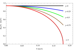
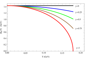
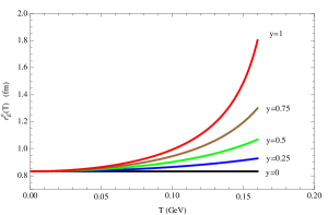
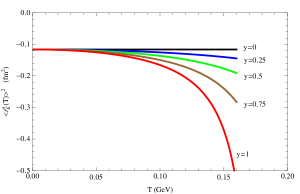
Figure 1: Temperature dependence of nucleon and Roper masses up to $T_{c}=230$ MeV.

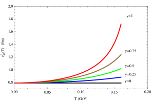
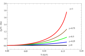
Figure 2: Temperature dependence of nucleon charge radii $r_{E}^{p}$ and $\langle r^{2}_{E}\rangle^{n}$ up to $T=200$ MeV.

Figure 3: Temperature dependence of nucleon magnetic radii $r_{M}^{p}$ and $r_{M}^{n}$ up to $T=200$ MeV.

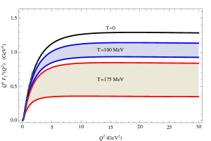
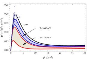
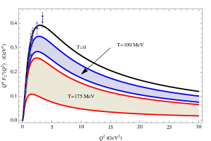
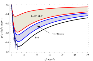
Figure 4: Temperature dependence of Dirac $u$ and $d$ quark form factors multiplied by $Q^{4}$.

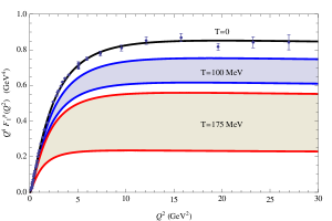
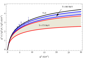
Figure 5: Temperature dependence of Pauli $u$ and $d$ quark form factors multiplied by $Q^{4}$.

Figure 6: Temperature dependence of Dirac proton form factor multiplied by $Q^{4}$ and of the ratio $Q^{2}F_{2}^{p}(Q^{2})/F_{1}^{p}(Q^{2})$.

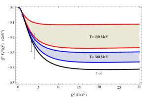
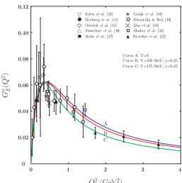
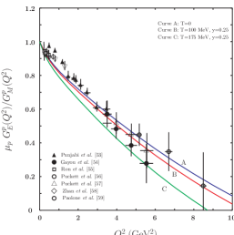
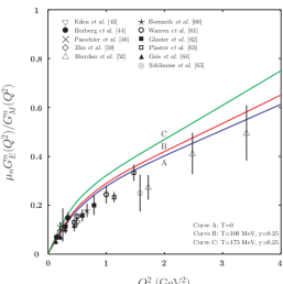
Figure 7: Temperature dependence of the Dirac neutron form factor multiplied by $Q^{4}$ and the charge neutron form factor $G_{E}^{n}(Q^{2})$ in comparison with data.

Figure 8: Temperature dependence of the ratios $\mu_{p}G_{E}^{p}(Q^{2})/G_{M}^{p}(Q^{2})$ and $\mu_{n}G_{E}^{n}(Q^{2})/G_{M}^{n}(Q^{2})$ in comparison with data.

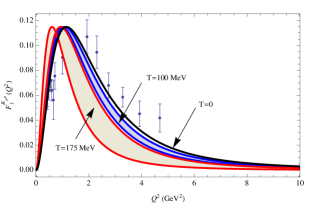
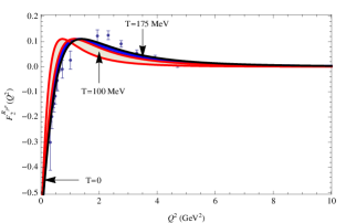
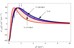
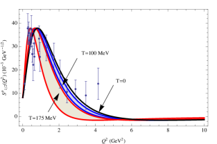
Figure 9: Temperature dependence of the Roper-nucleon transition form factors $F_{1}^{{\cal R}_{p}p}(Q^{2})$ and $F_{2}^{{\cal R}_{p}p}(Q^{2})$ up to 10 GeV².

Figure 10: Temperature dependence of the helicity amplitudes $A_{1/2}^{p}(Q^{2})$ and $S_{1/2}^{p}(Q^{2})$ up to 10 GeV².

References

- [1] I. Kirsch, JHEP 0609, 052 (2006).
- [2] Z. Abidin and C. E. Carlson, Phys. Rev. D 79, 115003 (2009).
- [3] A. Vega, I. Schmidt, T. Gutsche, and V. E. Lyubovitskij, Phys. Rev. D 83, 036001 (2011).
- [4] T. Gutsche, V. E. Lyubovitskij, I. Schmidt, and A. Vega, Phys. Rev. D 86, 036007 (2012).
- [5] S. J. Brodsky and G. R. Farrar, Phys. Rev. Lett. 31, 1153 (1973); V. A. Matveev, R. M. Muradian and A. N. Tavkhelidze, Lett. Nuovo Cim. 7, 719 (1973).
- [6] T. Gutsche, V. E. Lyubovitskij, I. Schmidt and A. Vega, Phys. Rev. D 85, 076003 (2012).
- [7] S. J. Brodsky, G. F. de Teramond, H. G. Dosch and J. Erlich, Phys. Rep. 584, 1 (2015).
- [8] R. S. Sufian, G. F. de Teramond, S. J. Brodsky, A. Deur, and H. G. Dosch, Phys. Rev. D 95, 014011 (2017).
- [9] E. Folco Capossoli, M. A. M. Contreras, D. Li, A. Vega and H. Boschi-Filho, arXiv:1903.06269 [hep-ph].
- [10] T. Gutsche, V. E. Lyubovitskij, I. Schmidt, and A. Vega, Phys. Rev. D 89, 054033 (2014), D 92, 019902(E) (2015); D 91, 054028 (2015).
- [11] T. Gutsche, V. E. Lyubovitskij and I. Schmidt, Eur. Phys. J. C 77, 86 (2017).
- [12] V. N. Gribov and L. N. Lipatov, Sov. J. Nucl. Phys. 15, 438 (1972) [Yad. Fiz. 15, 781 (1972)]; V. N. Gribov and L. N. Lipatov, Sov. J. Nucl. Phys. 15, 675 (1972) [Yad. Fiz. 15, 1218 (1972)]; G. Altarelli and G. Parisi, Nucl. Phys. B 126, 298 (1977); Y. L. Dokshitzer, Sov. Phys. JETP 46, 641 (1977) [Zh. Eksp. Teor. Fiz. 73, 1216 (1977)].
- [13] G. F. de Teramond and S. J. Brodsky, AIP Conf. Proc. 1432, 168 (2012).
- [14] T. Gutsche, V. E. Lyubovitskij, I. Schmidt, and A. Vega, Phys. Rev. D 87, 016017 (2013).
- [15] G. Ramalho and D. Melnikov, Phys. Rev. D 97, 034037 (2018); G. Ramalho, Phys. Rev. D 96, 054021 (2017).
- [16] T. Gutsche, V. E. Lyubovitskij and I. Schmidt, Phys. Rev. D 97, 054011 (2018).
- [17] T. Gutsche, V. E. Lyubovitskij, I. Schmidt and A. Y. Trifonov, Phys. Rev. D 99, 054030 (2019).
- [18] T. Gutsche, V. E. Lyubovitskij, I. Schmidt and A. Y. Trifonov, Phys. Rev. D 99, 114023 (2019).
- [19] J. Gasser and H. Leutwyler, Phys. Lett. B 184, 83 (1987).
- [20] H. Leutwyler, Nucl. Phys. Proc. Suppl. 4, 248 (1988); P. Gerber and H. Leutwyler, Nucl. Phys. B 321, 387 (1989).
- [21] D. Toublan, Phys. Rev. D 56, 5629 (1997).
- [22] A. Vega and M. A. Martin Contreras, Nucl. Phys. B 942, 410 (2019).
- [23] B. L. Ioffe, Nucl. Phys. B 188, 317 (1981), Nucl. Phys. B 191, 591(E) (1981).
- [24] A. W. Thomas and W. Weise, “The Structure of the Nucleon,” Berlin, Germany: Wiley-VCH (2001) 389 p.
- [25] A. Gorsky, P. N. Kopnin and A. Krikun, Phys. Rev. D 89, no. 2, 026012 (2014).
- [26] L. Y. Glozman, C. B. Lang and M. Schrock, Phys. Rev. D 86, 014507 (2012).
- [27] D. Diakonov, V. Y. Petrov and P. V. Pobylitsa, Nucl. Phys. B 306, 809 (1988).
- [28] Y. L. Ma, M. Harada, H. K. Lee, Y. Oh, B. Y. Park and M. Rho, Phys. Rev. D 90, 034015 (2014).
- [29] A. Gorsky, S. B. Gudnason and A. Krikun, Phys. Rev. D 91, 126008 (2015).
- [30] A. P. Trawinski, S. D. Glazek, S. J. Brodsky, G. F. de Teramond and H. G. Dosch, Phys. Rev. D 90, 074017 (2014).
- [31] T. Gutsche, V. E. Lyubovitskij, I. Schmidt and A. Vega, Phys. Rev. D 90, 096007 (2014).
- [32] D. Vercauteren and H. Verschelde, Phys. Rev. D 82, 085026 (2010).
- [33] H. Leutwyler, “Deconfinement and Chiral Symmetry”, in Proc. “QCD 20 Years Later, Vol. 2, P. M. Zerwas and H. A. Kastrup (Eds.), World Scientific, Singapore, 1993, 693.
- [34] D. E. Miller, Acta Phys. Polon. B 28, 2937 (1997).
- [35] H. R. Grigoryan and A. V. Radyushkin, Phys. Rev. D 76, 095007 (2007).
- [36] A. Kadeer, J. G. Körner and U. Moosbrugger, Eur. Phys. J. C 59, 27 (2009).
- [37] A. Faessler, T. Gutsche, M. A. Ivanov, J. G. Körner, and V. E. Lyubovitskij, Phys. Rev. D 80, 034025 (2009).
- [38] T. Branz, A. Faessler, T. Gutsche, M. A. Ivanov, J. G. Körner, V. E. Lyubovitskij, and B. Oexl, Phys. Rev. D 81, 114036 (2010).
- [39] T. Gutsche, M. A. Ivanov, J. G. Körner, V. E. Lyubovitskij, V. V. Lyubushkin, and P. Santorelli, Phys. Rev. D 96, 013003 (2017).
- [40] M. Tanabashi et al. (Particle Data Group), Phys. Rev. D 98, 030001 (2018).
- [41] G. D. Cates, C. W. de Jager, S. Riordan, and B. Wojtsekhowski, Phys. Rev. Lett. 106, 252003 (2011).
- [42] M. Diehl and P. Kroll, Eur. Phys. J. C 73, 2397 (2013); M. Diehl, Nucl. Phys. Proc. Suppl. 161, 49 (2006).
- [43] T. Eden, R. Madey, W. M. Zhang, B. D. Anderson,H. Arenhovel,A. R. Baldwin, D. Barkhuff,K. B. Beard, W. Bertozzi et al., Phys. Rev. C 50, R1749 (1994).
- [44] C. Herberg et al., Eur. Phys. J. A 5, 131 (1999).
- [45] M. Ostrick, C. Herberg, H. G. Andresen, J. R. M. Annand, K. Aulenbacher, J. Becker, P. Drescher, D. Eyl, A. Frey et al., Phys. Rev. Lett. 83, 276 (1999).
- [46] I. Passchier, R. Alarcon, T. S. Bauer, D. Boersma, J. F. J. van den Brand, L. D. van Buuren, H. J. Bulten, M. Ferro-Luzzi, P. Heimberg et al., Phys. Rev. Lett. 82, 4988 (1999).
- [47] D. Rohe et al., Phys. Rev. Lett. 83, 4257 (1999).
- [48] J. Golak, G. Ziemer, H. Kamada, H. Witala, and W. Glöckle, Phys. Rev. C 63, 034006 (2001).
- [49] R. Schiavilla and I. Sick, Phys. Rev. C 64, 041002(R) (2001).
- [50] H. Zhu et al. (Jefferson Lab E93-026 Collaboration), Phys. Rev. Lett. 87, 081801 (2001).
- [51] R. Madey et al. (Jefferson Lab E93-038 Collaboration), Phys. Rev. Lett. 91, 122002 (2003).
- [52] S. Riordan et al., Phys. Rev. Lett. 105, 262302 (2010).
- [53] V. Punjabi et al., Phys. Rev. C 71, 055202 (2005); C 71, 069902(E) (2005).
- [54] O. Gayou et al. (Jefferson Lab Hall A Collaboration), Phys. Rev. Lett. 88, 092301 (2002).
- [55] G. Ron et al. (JLab Hall A Collaboration), Phys. Rev. C 84, 055204 (2011).
- [56] A. J. R. Puckett et al., Phys. Rev. C 96, 055203 (2017)
- [57] A. J. R. Puckett et al., Phys. Rev. C 85, 045203 (2012).
- [58] X. Zhan et al., Phys. Lett. B 705, 59 (2011).
- [59] M. Paolone et al., Phys. Rev. Lett. 105, 072001 (2010).
- [60] J. Bermuth et al., Phys. Lett. B 564, 199 (2003).
- [61] G. Warren et al. (Jefferson Laboratory E93-026 Collaboration), Phys. Rev. Lett. 92, 042301 (2004).
- [62] D. I. Glazier et al., Eur. Phys. J. A 24, 101 (2005)
- [63] B. Plaster et al. (Jefferson Laboratory E93-038 Collaboration), Phys. Rev. C 73, 025205 (2006).
- [64] E. Geis, M. Kohl, V. Ziskin, T. Akdogan, H. Arenhovel, R. Alarcon, W. Bertozzi, E. Booth, T. Botto et al. (BLAST Collaboration), Phys. Rev. Lett. 101, 042501 (2008).
- [65] B. S. Schlimme, P. Achenbach, C. A. Ayerbe Gayoso, J. C. Bernauer, R. Bohm, D. Bosnar, T. Challand, M. O. Distler, L. Doria, F. Fellenberger et al., Phys. Rev. Lett. 111, 132504 (2013).
- [66] I. G. Aznauryan et al. (CLAS Collaboration), Phys. Rev. C 80, 055203 (2009).
- [67] I. G. Aznauryan and V. D. Burkert, Phys. Rev. C 85, 055202 (2012).
- [68] V. I. Mokeev et al., Phys. Rev. C 93, 025206 (2016).
- [69] S. Stajner, P. Achenbach, T. Beranek, J. Bericic, J. C. Bernauer, D. Bosnar, R. Bohm, L. Correa, A. Denig et al., Phys. Rev. Lett. 119, 022001 (2017).
- [70] C. A. Dominguez, M. Loewe and J. S. Rozowsky, Phys. Lett. B 335, 506 (1994).