Control of eigenfunctions
on surfaces of variable curvature

Abstract.

We prove a microlocal lower bound on the mass of high energy eigenfunctions of the Laplacian on compact surfaces of negative curvature, and more generally on surfaces with Anosov geodesic flows. This implies controllability for the Schrödinger equation by any nonempty open set, and shows that every semiclassical measure has full support. We also prove exponential energy decay for solutions to the damped wave equation on such surfaces, for any nontrivial damping coefficient. These results extend previous works [DJ18, Ji20], which considered the setting of surfaces of constant negative curvature.

The proofs use the strategy of [DJ18, Ji20] and rely on the fractal uncertainty principle of [BD18]. However, in the variable curvature case the stable/unstable foliations are not smooth, so we can no longer associate to these foliations a pseudodifferential calculus of the type used in [DZ16]. Instead, our argument uses Egorov’s Theorem up to local Ehrenfest time and the hyperbolic parametrix of [NZ09], together with the $C^{1+}$ regularity of the stable/unstable foliations.

Let $(M,g)$ be a compact smooth Riemannian manifold. The Laplace–Beltrami operator $\Delta$ admits a complete set of eigenfunctions

$$u_{j}\in C^{\infty}(M),\quad(-\Delta-\lambda_{j}^{2})u_{j}=0,\quad\|u_{j}\|_{L^{2}(M)}=1.$$

These can be interpreted as stationary states of a quantum particle evolving freely on $M$, with $\lambda_{j}^{2}$ being the energy of the particle, and $|u_{j}(x)|^{2}$ the probability density of finding the particle at the point $x$. One fundamental question in the field of spectral geometry is to understand the structure of the eigenfunctions $u_{j}$ in the high-energy régime $\lambda_{j}\to\infty$, using some information on the geodesic flow on $M$ (this flow corresponds to the dynamics of a classical particle evolving freely on $M$). In particular, the field of Quantum Chaos focuses on situations where the geodesic flow on $M$ has chaotic behavior.

In this paper we assume that $(M,g)$ is a compact connected Riemannian surface without boundary, whose geodesic flow has the Anosov property (see §2.1 for definitions and properties); we will refer to such $(M,g)$ as an Anosov surface. Anosov flows form a standard mathematical model of systems with strongly chaotic behavior, in some sense they are the “purest” form of chaotic systems. A large family of examples is provided by the surfaces of negative Gauss curvature. Our first result gives a lower bound on the mass distribution of $u_{j}$, showing that the probability of finding the quantum particle in any fixed open set is bounded away from zero uniformly in the high-energy limit:

Theorem 1.

Assume that $(M,g)$ is an Anosov surface. Choose $\Omega\subset M$ open and nonempty. Then there exists a constant $c_{\Omega}>0$ such that any eigenfunction $u_{j}$ of the Laplace–Beltrami operator on $(M,g)$ satisfies

$$\|u_{j}\|_{L^{2}(\Omega)}\geq c_{\Omega}\,.$$ (1.1)

On any Riemannian manifold, the unique continuation principle shows that a positive lower bound (1.1) holds if one allows $c_{\Omega}$ to depend on $\lambda_{j}$; see e.g. Lebeau–Robbiano [LR95, Corollaire 2]; an introduction to quantitative unique continuation for eigenfunctions of the Schrödinger operators on $\mathbb{R}^{d}$ can be found in [Zw12, Theorem 7.7]. In general, the lower bound decays exponentially fast as $\lambda_{j}\to\infty$, as can be seen in the case of the round sphere, where one can construct Gaussian beam eigenstates concentrating on a closed geodesic and exponentially small away from this geodesic. Note that related propagation of smallness results for solutions of elliptic equations were also obtained for any set $\Omega$ of positive Lebesgue measure $\operatorname{vol}(\Omega)$ by Logunov–Malinnikova [LM19, §1.7], who showed that

$$\sup_{\Omega}|u_{j}|\geq\bigg{(}{\operatorname{vol}(\Omega)\over C}\bigg{)}^{C\lambda_{j}}\sup_{M}|u_{j}|$$

for some constant $C$ depending on $(M,g)$, but not on $\Omega$ or $j$. In our situation, the energy-independent lower bound (1.1) strongly relies on the chaotic behavior of the geodesic flow.

The proof of Theorem 1 gives a stronger result featuring the localization of $u_{j}$ in both position and Fourier spaces. Let $\operatorname{Op}_{h}$ be a semiclassical quantization procedure on $M$, and $S^{0}(T^{*}M)$ be the standard symbol class, see §2.2. Denote by $S^{*}M\subset T^{*}M$ the cosphere bundle.

Theorem 2.

Assume that $a\in S^{0}(T^{*}M)$ and $a|_{S^{*}M}\not\equiv 0$. Then there exist constants $C>0$ and $h_{0}>0$ depending only on $a$, such that for all $h\in(0,h_{0})$ and all $u\in H^{2}(M)$ we have the estimate

$$\|u\|_{L^{2}(M)}\leq C\|\operatorname{Op}_{h}(a)u\|_{L^{2}(M)}+{C\log(1/h)\over h}\big{\|}(-h^{2}\Delta-I)u\big{\|}_{L^{2}(M)}.$$ (1.2)

If $a=a(x)$ is a function on $M$, then $\operatorname{Op}_{h}(a)$ is the multiplication operator by $a$. Hence Theorem 2 implies Theorem 1 by taking $a(x)$ supported inside $\Omega$ and putting $h:=\lambda_{j}^{-1}$, $u:=u_{j}$. More generally, the lower bound (1.1) holds for quasimodes $u_{h}$ of the Laplacian of the following type:

$$\|(-h^{2}\Delta-I)u_{h}\|_{L^{2}(M)}=o\big{(}h/\log(1/h)\big{)},\quad h\to 0;\quad\|u_{h}\|_{L^{2}(M)}=1.$$ (1.3)

On the opposite, the lower bound (1.1) may fail for quasimodes of error $\mathcal{O}(h/\log(1/h))$: for $(M,g)$ a surface of constant negative curvature (also known as a hyperbolic surface), Brooks [Br15] constructed quasimodes of such strength localized along a closed geodesic; the construction was extended to more general two-dimensional quantum systems by Eswarathasan–Nonnenmacher [EN17], and in higher dimension to quasimodes localized on an invariant submanifold of $M$ by Eswarathasan–Silberman [ES17].

1.1. Application to semiclassical measures

We now discuss two applications of Theorem 2. The first one concerns semiclassical measures, which describe asymptotic macroscopic distribution of subsequences of eigenfunctions. More precisely, if $(u_{j_{k}})_{k\in\mathbb{N}}$ is a sequence of eigenfunctions with $\lambda_{j_{k}}\to\infty$ and $h_{j_{k}}:=\lambda_{j_{k}}^{-1}$, then we say that $(u_{j_{k}})_{k}$ converges to a measure $\mu$ on $T^{*}M$ if

$$\langle\operatorname{Op}_{h_{j_{k}}}(a)u_{j_{k}},u_{j_{k}}\rangle_{L^{2}(M)}\xrightarrow{k\to\infty}\int_{T^{*}M}a\,d\mu\quad\text{for all}\quad a\in S^{0}(T^{*}M).$$ (1.4)

The measure $\mu$ is called a semiclassical measure of the manifold $(M,g)$, it describes the asymptotic microlocal properties of the eigenstates along the sequence $(u_{j_{k}})$ of eigenfunctions. A compactness argument shows that, from any sequence of eigenstates $(u_{j_{k}})$, it is always possible to extract a subsequence which converges to a semiclassical measure. Any semiclassical measure is a probability measure supported inside $S^{*}M$, which is invariant under the geodesic flow, see [Zw12, Chapter 5].

From (1.4) and the semiclassical calculus we see that $\|\operatorname{Op}_{h_{j_{k}}}(a)u_{j_{k}}\|_{L^{2}(M)}^{2}$ converges to $\int|a|^{2}\,d\mu$. Thus Theorem 2 implies the following

Theorem 3.

Let $\mu$ be a semiclassical measure associated to a sequence of Laplacian eigenfunctions on $M$. Then $\operatorname{supp}\mu=S^{*}M$, that is $\mu(U)>0$ for any open nonempty $U\subset S^{*}M$.

While we do not provide an explicit formula for the lower bound on $\mu(U)$ in terms of $U$, we show that this lower bound only depends on a certain dynamical quantity associated to $U$:

Theorem 4.

There exists $\varepsilon_{0}>0$ depending only on $(M,g)$ such that the following holds. Assume that $U\subset S^{*}M$ is an open set which is $(L_{0},L_{1})$-dense in both unstable and stable directions in the sense of Definition 2.16 below, and has diameter less than $\varepsilon_{0}$. Then for each semiclassical measure $\mu$ we have $\mu(U)\geq c$, where the constant $c>0$ depends only on $(M,g)$ and on the lengths $(L_{0},L_{1})$.

Theorem 4 follows by analyzing the dependence of various parameters in the proof of Theorem 2. We indicate the required changes in various remarks throughout the paper, with the proof of Theorem 4 explained at the end of §3.3.4. Let us remark that Theorems 3 and 4 also apply to semiclassical measures associated with quasimodes of the form (1.3).

We believe that our results are not specific to the Laplacian, but can be extended to operators of the form $P=-\Delta+P_{1}+P_{0}$ on $(M,g)$, where $P_{i}$ are symmetric differential operators of order $i$ with smooth coefficients. ‘ One could also consider semiclassical Schrödinger operators $P_{h}=-h^{2}\Delta+V$ with $V\in C^{\infty}(M;\mathbb{R})$, and study families of eigenstates $P_{h}u_{h}=E(h)u_{h}$, with eigenvalues $E(h)\to 1$ when $h\to 0$. If the potential $V$ is sufficiently small, the Hamiltonian flow generated by the symbol $p(x,\xi)=|\xi|^{2}_{g}+V(x)$, restricted to the energy hypersurface $p^{-1}(1)$, will still enjoy the Anosov property, due to the structural stability of that property. We then believe that the eigenstates $(u_{h})_{h\to 0}$, as well as the associated semiclassical measures, will satisfy similar delocalization properties as in Theorems 1–4.

To put Theorems 2–4 into context, let us give a brief historical review, referring to the expository articles of Marklof [Ma06], Zelditch [Ze09], and Sarnak [Sa11] for more information. The Quantum Ergodicity theorem of Shnirelman [Sh74a, Sh74b], Zelditch [Ze87], and Colin de Verdière [CdV85] states that when the geodesic flow on $S^{*}M$ is ergodic (with respect to the Liouville measure $\mu_{L}$), there exists a density one sequence $(u_{j_{k}})$ which asymptotically equidistributes, namely which converges to the Liouville measure $\mu_{L}$ in the sense of (1.4). The Quantum Unique Ergodicity (QUE) conjecture formulated by Rudnick–Sarnak [RS94] states that on any Anosov manifold, the full sequence of eigenfunctions equidistributes, that is $\mu_{L}$ is the unique semiclassical measure. So far this conjecture has only been established for hyperbolic surfaces possessing arithmetic symmetries [Li06]. On the other hand, there exist toy models of quantized Anosov maps on the two-dimensional torus, where the corresponding QUE conjecture fails, see Faure–Nonnenmacher–de Bièvre [FNdB03] and Anantharaman–Nonnenmacher [AN07b]. On a similar Anosov toy model on a higher dimensional torus, Kelmer [Ke10] exhibited counterexamples to QUE, but also to our full delocalization result, featuring semiclassical measure supported on proper submanifolds.

With QUE seeming out of reach, it is natural to wonder which flow invariant probability measures on $S^{*}M$ can arise as semiclassical measures; in other words, does quantum mechanics select certain invariant measures, or allow all of them? The first restrictions on semiclassical measures were proved by Anantharaman [An08], Anantharaman–Nonnenmacher [AN07a], Rivière [Ri10], and Anantharaman–Silberman [AS13], in the form of positive lower bounds on the Kolmogorov–Sinai entropy of $\mu$. The entropy is a nonnegative number associated with each invariant measure, representing the information theoretic complexity of the measure. Low-entropy measures therefore have low complexity. These lower bounds on the entropy exclude, for instance, the extreme case when $\mu$ is a $\delta$ measure on a closed geodesic. Our Theorem 3 gives a different type of restriction on $\mu$. As explained in [DJ18], there exist invariant measures which are excluded by Theorem 3 but not by entropy bounds, and vice versa. For instance, on any Anosov surface one can construct flow invariant fractal subsets $F\subsetneq S^{*}M$ of Hausdorff dimension close to $3$, which support invariant measures of large entropy. Conversely, an invariant measure of the form $\epsilon\mu_{L}+(1-\epsilon)\delta_{\gamma}$, with $\delta_{\gamma}$ the delta measure on a closed geodesic and $0<\epsilon\ll 1$, will have full support but small entropy.

In the special case of hyperbolic surfaces, Theorems 1–3 were proved by Dyatlov–Jin [DJ18]; see also the reviews [Dy17, Dy19]. The proofs in the present paper partially use the strategy of [DJ18], in particular they rely on the fractal uncertainty principle (FUP) established by Bourgain–Dyatlov [BD18]. However, many new difficulties arise in the variable curvature case, in particular from the fact that the stable and unstable foliations on $S^{*}M$ are not smooth, see §§1.4,4.1 below.

1.2. Application to control theory

The second application of Theorem 2 is to observability and exact null-controllability for the (nonsemiclassical) Schrödinger equation:

Theorem 5.

Assume that $\Omega\subset M$ is open and nonempty, and fix $T>0$. Then:

• (Observability) There exists a constant $K>0$ depending only on $M$, $\Omega$, and $T$, such that for any $u_{0}\in L^{2}(M)$, we have

  $$\|u_{0}\|_{L^{2}(M)}^{2}\leq K\int_{0}^{T}\|e^{it\Delta}u_{0}\|_{L^{2}(\Omega)}^{2}dt;$$ (1.5)

• (Control) For any $u_{0}\in L^{2}(M)$, there exists $f\in L^{2}((0,T)\times\Omega)$ such that the solution to the equation

  $$(i\partial_{t}+\Delta)u(t,x)=f\mathbf{1}_{(0,T)\times\Omega}(t,x),\quad u(0,x)=u_{0}(x)$$

  satisfies

  $$u(T,x)\equiv 0.$$

The proof that the above statements follow from Theorem 2 is identical to the one in Jin [Ji18], so we will not reproduce it here.

For a general manifold, such observability/control is known to hold if the open set $\Omega$ satisfies the geometric control condition of Bardos–Lebeau–Rauch [BLR92, Le92], namely if every geodesic ray intersects $\Omega$. Yet, it may hold as well if this geometric condition is violated, for instance on compact manifolds of negative sectional curvature, provided the set of geodesics never meeting $\Omega$ is “sufficiently thin”, see Anantharaman–Rivière [AR12]. The novelty in the above two-dimensional result, is that this control holds for any open set $\Omega$, now matter how thick the set of uncontrolled geodesics. So far the only other family of manifolds for which observability/control was known to hold for any $\Omega$ were the flat tori, see Haraux [Ha89] and Jaffard [Ja90]. Further references on this question may be found in Burq–Zworski [BZ04] and Jin [Ji18].

1.3. Damped wave equation

Our final result concerns the long time behavior of solutions to the damped wave equation on $M$, with damping function $b\in C^{\infty}(M)$, $b\geq 0$, $b\not\equiv 0$:

$$(\partial_{t}^{2}-\Delta+2b(x)\partial_{t})v(t,x)=0,\quad v|_{t=0}=v_{0}(x),\quad\partial_{t}v|_{t=0}=v_{1}(x).$$ (1.6)

Semigroup theory shows that for initial data $(v_{0},v_{1})\in\mathcal{H}^{0}:=H^{1}(M)\times L^{2}(M)$, the above equation has a unique solution in $C(\mathbb{R}^{+};H^{1}(M))\cap C^{1}(\mathbb{R}^{+};L^{2}(M))$. The energy of this solution at time $t\geq 0$ is defined by

$$E(v(t)):=\frac{1}{2}\int_{M}|\partial_{t}v(t,x)|^{2}+|\nabla_{x}v(t,x)|^{2}\,dx.$$ (1.7)

It is well-known that on every compact Riemannian manifold, this energy decays to zero when $t\to\infty$. However, the rate of decay depends on a subtle interplay between the geodesic flow and the support of the damping function, see Lebeau [Le96]. In particular, exponential decay (the fastest possible decay) always holds if the damping function satisfies the geometric control condition, that is any geodesic intersects the set $\{b>0\}$. In the case of an Anosov surface with any damping function $b$, we obtain exponential decay without requiring this geometric condition:

Theorem 6.

Assume that $b\geq 0$ but $b\not\equiv 0$. Then for every $s>0$, there exist constants $C$ and $\gamma=\gamma(s)>0$ such that for any $(v_{0},v_{1})\in\mathcal{H}^{s}:=H^{s+1}(M)\times H^{s}(M)$, the energy of the solution decays exponentially:

$$E(v(t))\leq C\,e^{-\gamma t}\,\|(v_{0},v_{1})\|_{\mathcal{H}^{s}}^{2}\,.$$ (1.8)

We remark that on any compact manifold, the decay (1.8) holds for $s=0$ if and only if the set $\{b>0\}$ satisfies the geometric control condition, see Rauch–Taylor [RaTa75]. On manifolds of negative curvature, an exponential decay controlled by a higher Sobolev norm $s>0$ has been proved in situations where the set of undamped trajectories is sufficiently “thin”, see Schenck [Sc10].

To our knowledge, Theorem 6 gives the first class of manifolds (of dimension $\geq 2$) for which the energy decays exponentially (under a control by a higher Sobolev norm), no matter how small the support of the damping is. As a comparison, in the case of flat tori, in absence of geometric control of the region $\{b>0\}$, the decay is instead algebraic in time, see Anantharaman–Léautaud [AnLe14]. For an account on previous results on the rate of energy decay for damped waves, the reader may consult the introduction to [Ji20] and the references therein.

The proof of Theorem 6 uses many of the ingredients of the proof of Theorem 2, including the key estimate, Proposition 3.2. In the special case of hyperbolic surfaces, Theorem 6 was proved by Jin [Ji20] using the methods of [DJ18].

1.4. Structure of the article

• In §2 we review various ingredients used in the proof. Those include: hyperbolic (Anosov) dynamics and stable/unstable manifolds (§2.1); pseudodifferential operators with mildly exotic symbols and Egorov’s theorem (§2.2); Lagrangian distributions/Fourier integral operators (§2.3); fractal uncertainty principle (§2.4); proof of porosity of dynamically defined sets (§2.5).

• In §3 we give the proofs of Theorems 2, 4 (§3.3), and 6 (§3.4). The strategy of proof is similar to the one used in [DJ18, Ji20] in the constant curvature case. It starts from a microlocal partition of the identity, quantizing the partition of $S^{*}M$ into the controlled vs. uncontrolled regions. Using the wave group, we may refine this microlocal partition up to a time $N$, each element of the refined partition being an operator $A_{\mathbf{w}}=A_{w_{N}}(N)\cdots A_{w_{1}}(1)A_{w_{0}}$ indexed by a word $\mathbf{w}=w_{0}\ldots w_{N}$, each symbol $w_{j}$ indicating whether the system sits in the controlled or uncontrolled region at the time $j$. We need to push this refinement up to a time $N\sim C\log(1/h)$ exceeding the Ehrenfest time, which implies that the operators $A_{\mathbf{w}}$ are no longer pseudodifferential operators. The core of the proof then consists in a key estimate on these “long” operators $A_{\mathbf{w}}$, given in Proposition 3.2.

• §4 is devoted to the proof of this key Proposition. It proceeds by transforming this estimate into a collection of fractal uncertainty principles. This part of the proof is very different from the constant curvature case, due to the fact that the Ehrenfest time is not uniform, but depends on the trajectory; the difficulty also comes from the low regularity of the stable/unstable foliations, which are not $C^{\infty}$, but only $C^{2-\epsilon}$. An outline of the proof is provided in §4.1.

• In §5 we complete the analysis of the operators $A_{\mathbf{w}}$, by splitting them into more elementary pieces, which we may precisely analyze through a version of Egorov’s Theorem up to the local Ehrenfest time. Similar elementary pieces were already introduced in the proofs of entropic lower bounds [An08, NZ09, Ri10]; we will need a somewhat more precise description of these operators for our aims.

• Appendix A contains quantitative estimates for the semiclassical pseudodifferential calculus on a compact surface, used in §2.2 and §5.

2. Ingredients

In this section we review some of the ingredients used in the proof: hyperbolic dynamics (§2.1), semiclassical analysis (§§2.2–2.3), fractal uncertainty principle (§2.4), and porosity properties in the stable/unstable directions (§2.5).

2.1. Hyperbolic dynamics

Let $(M,g)$ be a compact connected Riemannian surface. Denote

$$T^{*}M\setminus 0 :=\{(x,\xi)\in T^{*}M\colon\xi\neq 0\},$$

$$S^{*}M :=\{(x,\xi)\in T^{*}M\colon|\xi|_{g}=1\}.$$

Define the smooth function

$$p:T^{*}M\setminus 0\to\mathbb{R},\quad p(x,\xi):=|\xi|_{g}.$$ (2.1)

The Hamiltonian flow of $p$,

$$\varphi_{t}:=\exp(tH_{p}):T^{*}M\setminus 0\to T^{*}M\setminus 0$$ (2.2)

is the homogeneous geodesic flow, note that it preserves $S^{*}M$.

We assume that the restriction of $\varphi_{t}$ to $S^{*}M$ is an Anosov flow, namely for each $\rho\in S^{*}M$ there is a splitting of the tangent space $T_{\rho}(S^{*}M)$ into one-dimensional spaces

$$T_{\rho}(S^{*}M)=E_{0}(\rho)\oplus E_{s}(\rho)\oplus E_{u}(\rho)$$

such that:

• $E_{0}(\rho)=\mathbb{R}H_{p}(\rho)$ is the flow direction;

• $E_{s},E_{u}$ are invariant under $d\varphi_{t}$;

• $E_{s}$ is stable and $E_{u}$ is unstable in the following sense: for any choice of continuous metric $|\bullet|$ on the fibers of $T(S^{*}M)$, there exist $C,\theta>0$ such that

  $$|d\varphi_{t}(\rho)v|\leq Ce^{-\theta|t|}|v|,\quad\begin{cases}v\in E_{s}(\rho),&t\geq 0;\\ v\in E_{u}(\rho),&t\leq 0.\end{cases}$$ (2.3)

The Anosov assumption holds in particular if $(M,g)$ has everywhere negative Gauss curvature, see [KH97, Theorem 17.6.2], [Kl95, Theorem 3.9.1], or [Dy18, Theorem 6 in §5.1]. In the present setting the dependence of the spaces $E_{s},E_{u}$ (and the stable/unstable manifolds defined in §2.1.1 below) on the base point $\rho$ is $C^{2-}$ but (unless $M$ has constant curvature) not $C^{2}$, see Remark 1 following Lemma 2.3.

Since $\varphi_{t}$ is a homogeneous Hamiltonian flow, it preserves the canonical 1-form $\xi\,dx$ (which is the symplectic dual of the dilation field $\xi\cdot\partial_{\xi}$). By (2.3) we see that $\xi\,dx$ annihilates $E_{s}\oplus E_{u}$, that is

$$E_{s}\oplus E_{u}=\ker(dp)\cap\ker(\xi\,dx).$$ (2.4)

We fix adapted metrics $|\bullet|_{s}$, $|\bullet|_{u}$, which are smooth Riemannian metrics on $S^{*}M$, so that the following stronger version of (2.3) holds for some $\Lambda_{0}>0$:

$$|d\varphi_{t}(\rho)v|_{s}\leq e^{-\Lambda_{0}|t|}|v|_{s}, \quad v\in E_{s}(\rho),\quad t\geq 0;$$ (2.5)

$$|d\varphi_{t}(\rho)v|_{u}\leq e^{-\Lambda_{0}|t|}|v|_{u}, \quad v\in E_{u}(\rho),\quad t\leq 0.$$

See for instance [Dy18, Lemma 4.7] for the construction of such metrics. By homogeneity we extend the spaces $E_{0},E_{s},E_{u}$ to $T^{*}M\setminus 0$. We also extend $|\bullet|_{s}$, $|\bullet|_{u}$ to homogeneous metrics of degree 0 on $T^{*}M\setminus 0$.

For each $\rho\in T^{*}M\setminus 0$ and $t\in\mathbb{R}$ we define the stable/unstable expansion rates (since $E_{s},E_{u}$ are one-dimensional these coincide with the stable/unstable Jacobians):

$$|d\varphi_{t}(\rho)v|_{s}=J^{s}_{t}(\rho)|v|_{s}, \quad v\in E_{s}(\rho);$$ (2.6)

$$|d\varphi_{t}(\rho)v|_{u}=J^{u}_{t}(\rho)|v|_{u}, \quad v\in E_{u}(\rho).$$

From the stable/unstable decomposition and the homogeneity of the flow we see that for all $\rho\in\{{1\over 4}\leq|\xi|_{g}\leq 4\}$ and all $t$

$$\|d\varphi_{t}(\rho)\|\leq CJ^{u}_{t}(\rho), \quad t\geq 0;$$ (2.7)

$$\|d\varphi_{t}(\rho)\|\leq CJ^{s}_{t}(\rho), \quad t\leq 0.$$

Since $E_{0}$ is spanned by $H_{p}$ and $E_{s},E_{u}$ are tangent to the level sets of $p$, we see that the weak stable/unstable spaces $E_{s}\oplus E_{0}$, $E_{u}\oplus E_{0}$ are Lagrangian with respect to the standard symplectic form $\omega$ on $T^{*}M\setminus 0$ and $E_{s}\oplus E_{u}$ is symplectic. Since $\varphi_{t}$ are symplectomorphisms, there exists a constant $C$ such that for all $\rho\in T^{*}M\setminus 0$ and $t\in\mathbb{R}$

$$C^{-1}\leq J^{s}_{t}(\rho)J^{u}_{t}(\rho)\leq C.$$ (2.8)

Moreover, $J^{s}_{t}$ and $J^{u}_{t}$ are invariant under a short time evolution by the flow $\varphi_{t}$ up to a multiplicative constant: for all $\rho\in T^{*}M\setminus 0$, $t^{\prime}\in[-1,1]$, and $t\in\mathbb{R}$

$$C^{-1}J^{s}_{t}(\rho)\leq J^{s}_{t}(\varphi_{t^{\prime}}(\rho))\leq CJ^{s}_{t}(\rho),\quad C^{-1}J^{u}_{t}(\rho)\leq J^{u}_{t}(\varphi_{t^{\prime}}(\rho))\leq CJ^{u}_{t}(\rho).$$ (2.9)

By (2.5), $J^{s}_{t}$ is exponentially decaying in time, and $J^{u}_{t}$ cannot grow faster than exponentially due to the compactness of $M$. As a result, there exist constants $0<\Lambda_{0}\leq\Lambda_{1}$ such that for all $\rho\in T^{*}M\setminus 0$

$$e^{\Lambda_{0}|t|}\leq J^{u}_{t}(\rho)\leq e^{\Lambda_{1}|t|}, \quad e^{-\Lambda_{1}|t|}\leq J^{s}_{t}(\rho)\leq e^{-\Lambda_{0}|t|} \quad\text{for all}\quad t\geq 0;$$ (2.10)

$$e^{-\Lambda_{1}|t|}\leq J^{u}_{t}(\rho)\leq e^{-\Lambda_{0}|t|}, \quad e^{\Lambda_{0}|t|}\leq J^{s}_{t}(\rho)\leq e^{\Lambda_{1}|t|} \quad\text{for all}\quad t\leq 0.$$

For technical reasons (in the proof of Lemma 3.1) we choose to take $\Lambda_{1}\geq 1$.

Define also

$$\Lambda:=\bigg{\lceil}{\Lambda_{1}\over\Lambda_{0}}\bigg{\rceil}\in\mathbb{N}.$$ (2.11)

2.1.1. Stable/unstable manifolds

For $\rho\in S^{*}M$, denote by

$$W_{s}(\rho),W_{u}(\rho)\subset S^{*}M$$

the local stable/unstable leaves passing through $\rho$. These are $C^{\infty}$-embedded one dimensional disks (i.e. intervals) tangent to $E_{s}$, $E_{u}$. Their definition depends on arbitrary choices (because of the freedom of choosing where to end the interval) however their behavior near each point depends only on $(M,g)$. For the construction of $W_{s}(\rho),W_{u}(\rho)$ and their properties we refer to [KH97, Theorem 17.4.3], [Kl95, Theorem 3.9.2], or [Dy18, Theorem 5 in §4.6]. We can ajust the definition of these local laves such that they satisfy the following invariance properties under the flow $\varphi_{t}$:

$$\forall\rho\in S^{*}M,\qquad\varphi_{1}(W_{s}(\rho))\subset W_{s}(\varphi_{1}(\rho)),\quad\varphi_{-1}(W_{u}(\rho))\subset W_{u}(\varphi_{-1}(\rho)).$$ (2.12)

We also use the local weak stable/unstable leaves

$$W_{0s}(\rho):=\bigcup_{|t|\leq\tilde{\varepsilon}}\varphi_{t}(W_{s}(\rho)),\quad W_{0u}(\rho):=\bigcup_{|t|\leq\tilde{\varepsilon}}\varphi_{t}(W_{u}(\rho)),$$ (2.13)

which are $C^{\infty}$-embedded two dimensional rectangles inside $S^{*}M$ tangent to the weak stable/unstable spaces $E_{0}\oplus E_{s}$, $E_{0}\oplus E_{u}$. Here $\tilde{\varepsilon}>0$ is fixed small, depending only on $(M,g)$. We extend $W_{s},W_{u},W_{0s},W_{0u}$ to $T^{*}M\setminus 0$ by homogeneity, however for simplicity the lemmas below are stated on $S^{*}M$.

The stable/unstable manifolds are related to the dynamics of $\varphi_{t}$ by the following lemma. To state it we introduce the following piece of notation: for $A,B>0$

$$A\sim B\quad\text{iff}\quad C^{-1}A\leq B\leq CA\quad\text{for some}\ C>0\ \text{depending only on}\ (M,g).$$ (2.14)

Lemma 2.1.

Fix a Riemannian metric on $S^{*}M$ which induces a distance function $d(\bullet,\bullet)$. Then there exist $C,\varepsilon_{0}>0$ such that for all $\rho,\tilde{\rho}\in S^{*}M$ we have:

1. if $\tilde{\rho}\in W_{s}(\rho)$, then

   $$d(\varphi_{t}(\rho),\varphi_{t}(\tilde{\rho}))\leq CJ^{s}_{t}(\rho)d(\rho,\tilde{\rho})\quad\text{for all}\quad t\geq 0;$$ (2.15)

2. if $\tilde{\rho}\in W_{u}(\rho)$, then

   $$d(\varphi_{t}(\rho),\varphi_{t}(\tilde{\rho}))\leq CJ^{u}_{t}(\rho)d(\rho,\tilde{\rho})\quad\text{for all}\quad t\leq 0;$$ (2.16)

3. if $\tilde{\rho}\in W_{0s}(\rho)$, then $J^{s}_{t}(\rho)\sim J^{s}_{t}(\tilde{\rho})$ and $J^{u}_{t}(\rho)\sim J^{u}_{t}(\tilde{\rho})$ for all $t\geq 0$;

4. if $\tilde{\rho}\in W_{0u}(\rho)$, then $J^{s}_{t}(\rho)\sim J^{s}_{t}(\tilde{\rho})$ and $J^{u}_{t}(\rho)\sim J^{u}_{t}(\tilde{\rho})$ for all $t\leq 0$;

5. if $T\in\mathbb{N}_{0}$ and $d(\varphi_{t}(\rho),\varphi_{t}(\tilde{\rho}))\leq\varepsilon_{0}$ for all integers $t\in[0,T]$, then

   $$d(\tilde{\rho},W_{0s}(\rho))\leq{C/J^{u}_{T}(\rho)}$$ (2.17)

   and $J^{s}_{t}(\rho)\sim J^{s}_{t}(\tilde{\rho})$, $J^{u}_{t}(\rho)\sim J^{u}_{t}(\tilde{\rho})$ for all $t\in[0,T]$;

6. if $T\in\mathbb{N}_{0}$ and $d(\varphi_{t}(\rho),\varphi_{t}(\tilde{\rho}))\leq\varepsilon_{0}$ for all integers $t\in[-T,0]$, then

   $$d(\tilde{\rho},W_{0u}(\rho))\leq{C/J^{s}_{-T}(\rho)}$$ (2.18)

   and $J^{s}_{t}(\rho)\sim J^{s}_{t}(\tilde{\rho})$, $J^{u}_{t}(\rho)\sim J^{u}_{t}(\tilde{\rho})$ for all $t\in[-T,0]$.

Remarks. 1. The difference between Lemma 2.1 and standard facts from hyperbolic dynamics (see for instance [KH97, Theorem 17.4.3]) is that our estimates involve the local expansion rates for the point $\rho$ rather than the minimal expansion rate. This will be important later in our analysis.

2. By (2.8) we have $J^{s}_{t}(\rho)\sim 1/J^{u}_{t}(\rho)$. However the present lemma does not rely on $\varphi_{t}$ being symplectomorphisms which is why we choose to keep both the stable and unstable Jacobians in the estimates.

Proof.

We only prove parts (1), (3), (5), with parts (2), (4), (6) proved similarly.

(1) Without loss of generality we may assume that the distance function $d(\bullet,\bullet)$ is induced by the metric $|\bullet|_{s}$ used in (2.6) to define $J^{s}_{t}(\rho)$. Since the tangent space to $W_{s}(\rho)$ at $\rho$ is $E_{s}(\rho)$, there exists a constant $C$ such that for every $\rho\in S^{*}M$ and $\tilde{\rho}\in W_{s}(\rho)$

$$\big{|}d(\varphi_{1}(\rho),\varphi_{1}(\tilde{\rho}))-J^{s}_{1}(\rho)d(\rho,\tilde{\rho})\big{|}\leq Cd(\rho,\tilde{\rho})^{2}.$$ (2.19)

That is, when $\tilde{\rho}$ is close to $\rho$ the dilation factor of the distance $d(\rho,\tilde{\rho})$ by the map $\varphi_{1}$ is well-approximated by the norm of the differential $d\varphi_{1}(\rho)$ on $E_{s}(\rho)$.

Since $\tilde{\rho}\in W_{s}(\rho)$, there exist constants $C,\theta>0$ such that (see for instance [KH97, Theorem 17.4.3(3)] or [Dy18, (4.67)])

$$d(\varphi_{t}(\rho),\varphi_{t}(\tilde{\rho}))\leq Ce^{-\theta t}d(\rho,\tilde{\rho})\quad\text{for all}\quad t\geq 0.$$ (2.20)

For each integer $t\geq 0$, we have $\varphi_{t}(\tilde{\rho})\in W_{s}(\varphi_{t}(\rho))$ by (2.12). Applying (2.19) with $\rho,\tilde{\rho}$ replaced by $\varphi_{t}(\rho),\varphi_{t}(\tilde{\rho})$ we have

$$d(\varphi_{t+1}(\rho),\varphi_{t+1}(\tilde{\rho})) \leq J^{s}_{1}(\varphi_{t}(\rho))d(\varphi_{t}(\rho),\varphi_{t}(\tilde{\rho}))+Cd(\varphi_{t}(\rho),\varphi_{t}(\tilde{\rho}))^{2}$$ (2.21)

$$\leq(1+Ce^{-\theta t})J^{s}_{1}(\varphi_{t}(\rho))d(\varphi_{t}(\rho),\varphi_{t}(\tilde{\rho})).$$

By the chain rule we have for all integers $t\geq 0$

$$J^{s}_{t}(\rho)=J^{s}_{1}(\rho)J^{s}_{1}(\varphi_{1}(\rho))\cdots J^{s}_{1}(\varphi_{t-1}(\rho)).$$ (2.22)

Iterating (2.21) and using that the product $\prod_{j=0}^{\infty}(1+Ce^{-\theta j})$ converges, we get (2.15) for all integer $t\geq 0$, which immediately implies it for all $t\geq 0$.

(3) We show that $J^{s}_{t}(\rho)\sim J^{s}_{t}(\tilde{\rho})$, with the statement $J^{u}_{t}(\rho)\sim J^{u}_{t}(\tilde{\rho})$ proved similarly. Assume first that $\tilde{\rho}\in W_{s}(\rho)$. The map $\rho\mapsto E_{s}(\rho)$ is in the Hölder class $C^{\gamma}$ for some $\gamma>0$ (see for instance [Dy18, Lemma 4.3]; in §2.1.2 below we see that in our setting it is in fact $C^{2-}$). Recalling (2.6) we have for all $\rho,\tilde{\rho}\in S^{*}M$

$$|J^{s}_{1}(\rho)-J^{s}_{1}(\tilde{\rho})|\leq Cd(\rho,\tilde{\rho})^{\gamma}.$$

Applying this with $\rho$, $\tilde{\rho}$ replaced by $\varphi_{t}(\rho)$, $\varphi_{t}(\tilde{\rho})$ and using (2.20) we get for all $t\geq 0$

$$(1+Ce^{-\gamma\theta t})^{-1}J^{s}_{1}(\varphi_{t}(\rho))\leq J^{s}_{1}(\varphi_{t}(\tilde{\rho}))\leq(1+Ce^{-\gamma\theta t})J^{s}_{1}(\varphi_{t}(\rho)).$$ (2.23)

Using the chain rule (2.22) and iterating (2.23), we get $J^{s}_{t}(\rho)\sim J^{s}_{t}(\tilde{\rho})$ for all $t\geq 0$. The general weak stable case $\tilde{\rho}\in W_{0s}(\rho)$ follows since $J^{s}_{t}(\varphi_{t^{\prime}}(\rho))\sim J^{s}_{t}(\rho)$ for all $\rho\in S^{*}M$ and $t^{\prime}\in[-1,1]$ by (2.9).

(5) Since $E_{0}\oplus E_{s}$ is transversal to $E_{u}$, for $\varepsilon_{0}$ small enough and all $\rho,\tilde{\rho}\in S^{*}M$ such that $d(\rho,\tilde{\rho})\leq\varepsilon_{0}$, there exists a point (see Figure 1)

Figure 1. Left: the points $\rho,\tilde{\rho},\rho^{\prime}$ in the proof of part (5) of Lemma 2.1, with the flow direction removed. Right: the image of the left half by $\varphi_{T}$.

$$\rho^{\prime}\in W_{0s}(\rho)\cap W_{u}(\tilde{\rho}),\quad d(\rho,\rho^{\prime})\leq C\varepsilon_{0}.$$ (2.24)

See for instance [KH97, Proposition 6.4.13] (in the related case of maps) or [Dy18, (4.66)]. Since $\rho^{\prime}\in W_{0s}(\rho)$, by (2.20) there exists a constant $C_{0}\geq 1$ such that

$$d(\varphi_{t}(\rho^{\prime}),\varphi_{t}(\rho))\leq C_{0}\varepsilon_{0}\quad\text{for all}\quad t\geq 0.$$ (2.25)

By (2.12), for $\varepsilon_{0}$ small enough we have (denoting by $B_{d}$ balls with respect to the distance function $d(\bullet,\bullet)$)

$$\varphi_{1}(W_{u}(\hat{\rho}))\cap B_{d}(\varphi_{1}(\hat{\rho}),2C_{0}\varepsilon_{0})\subset W_{u}(\varphi_{1}(\hat{\rho}))\quad\text{for all}\quad\hat{\rho}\in S^{*}M.$$ (2.26)

Now, assume that $\rho,\tilde{\rho}\in S^{*}M$ and $d(\varphi_{t}(\rho),\varphi_{t}(\tilde{\rho}))\leq\varepsilon_{0}$ for all integers $t\in[0,T]$. Choose $\rho^{\prime}$ satisfying (2.24). If $\varepsilon_{0}$ is small enough, then by the local uniqueness of unstable leaves we have $\tilde{\rho}\in W_{u}(\rho^{\prime})$. By (2.25) we have for all integers $t\in[0,T]$

$$d(\varphi_{t}(\rho^{\prime}),\varphi_{t}(\tilde{\rho}))\leq d(\varphi_{t}(\rho^{\prime}),\varphi_{t}(\rho))+d(\varphi_{t}(\rho),\varphi_{t}(\tilde{\rho}))\leq 2C_{0}\varepsilon_{0}.$$

Applying (2.26) with $\hat{\rho}:=\varphi_{t}(\rho^{\prime})$, we see by induction on $t$ that

$$\varphi_{t}(\tilde{\rho})\in W_{u}(\varphi_{t}(\rho^{\prime}))\quad\text{for all integer}\quad t\in[0,T].$$

In particular, $\varphi_{T}(\tilde{\rho})\in W_{u}(\varphi_{T}(\rho^{\prime}))$. Applying (2.16) with $t:=-T$ and $\rho,\tilde{\rho}$ replaced by $\varphi_{T}(\rho^{\prime}),\varphi_{T}(\tilde{\rho})$,

$$d(\rho^{\prime},\tilde{\rho})=d\big{(}\varphi_{-T}(\varphi_{T}(\rho^{\prime})),\varphi_{-T}(\varphi_{T}(\tilde{\rho}))\big{)}\leq{CJ^{u}_{-T}(\varphi_{T}(\rho^{\prime}))}={C\over J^{u}_{T}(\rho^{\prime})}\leq{C\over J^{u}_{T}(\rho)}$$

where the last inequality follows from part (3) of the present lemma. Since $\rho^{\prime}\in W_{0s}(\rho)$ this proves (2.17).

It remains to show that $J^{s}_{t}(\rho)\sim J^{s}_{t}(\tilde{\rho})$, $J^{u}_{t}(\rho)\sim J^{u}_{t}(\tilde{\rho})$ for all $t\in[0,T]$. As before, we prove the first statement with the second one proved similarly. We can moreover restrict ourselves to integer values of $t$. By part (4) of the present lemma applied to the points $\varphi_{t}(\rho^{\prime})$, $\varphi_{t}(\tilde{\rho})\in W_{u}(\varphi_{t}(\rho^{\prime}))$ and propagation time $-t$, we have $J^{s}_{-t}(\varphi_{t}(\rho^{\prime}))\sim J^{s}_{-t}(\varphi_{t}(\tilde{\rho}))$. Since $J^{s}_{t}(\rho^{\prime})=1/J^{s}_{-t}(\varphi_{t}(\rho^{\prime}))$ this implies that $J^{s}_{t}(\rho^{\prime})\sim J^{s}_{t}(\tilde{\rho})$. On the other hand by part (3) of the present lemma we have $J^{s}_{t}(\rho)\sim J^{s}_{t}(\rho^{\prime})$. Combining the last two statements we get $J^{s}_{t}(\rho)\sim J^{s}_{t}(\tilde{\rho})$ as needed. ∎

Parts (5) and (6) of Lemma 2.1 applied to $\tilde{\rho}:=\varphi_{t}(\rho)$ together with (2.10) give

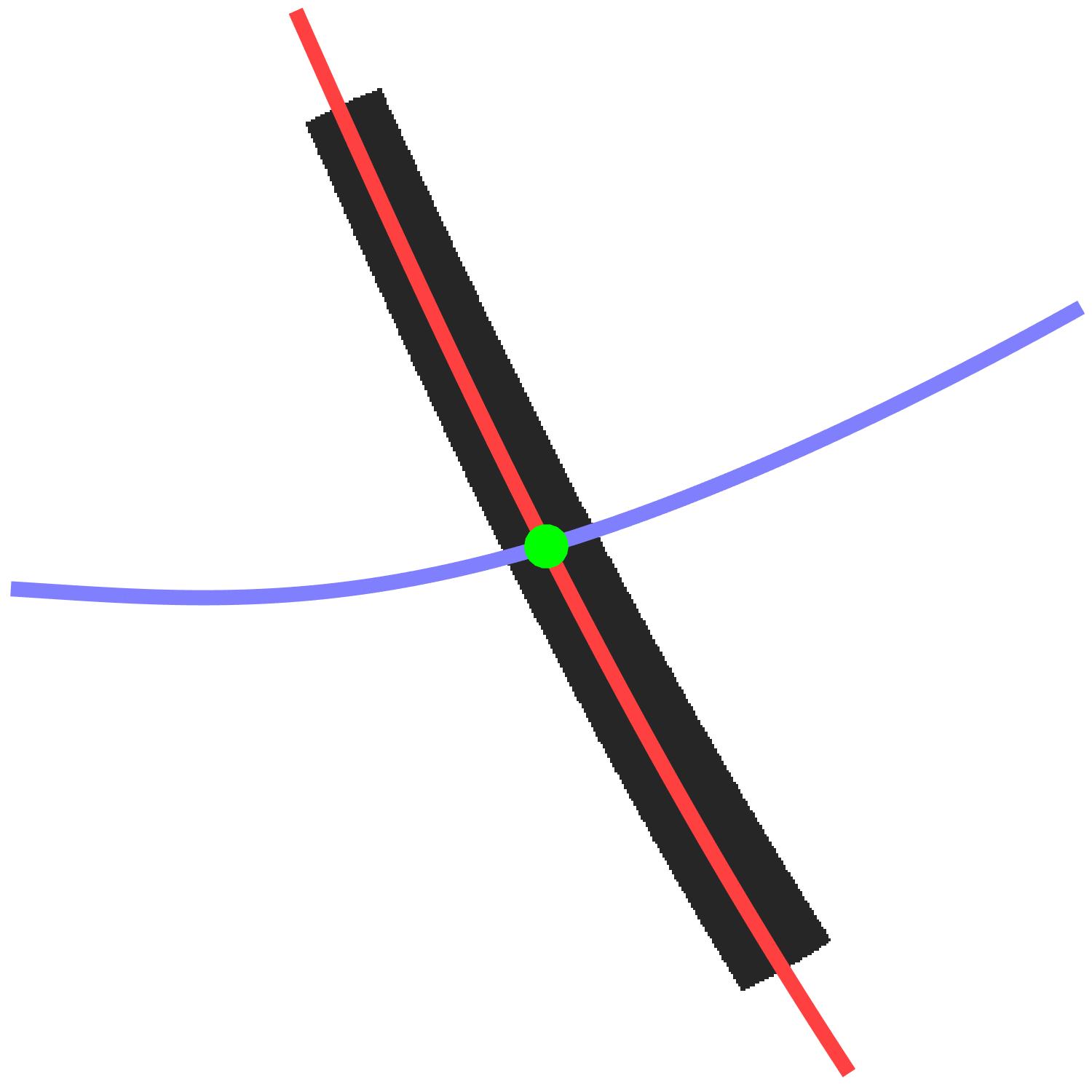
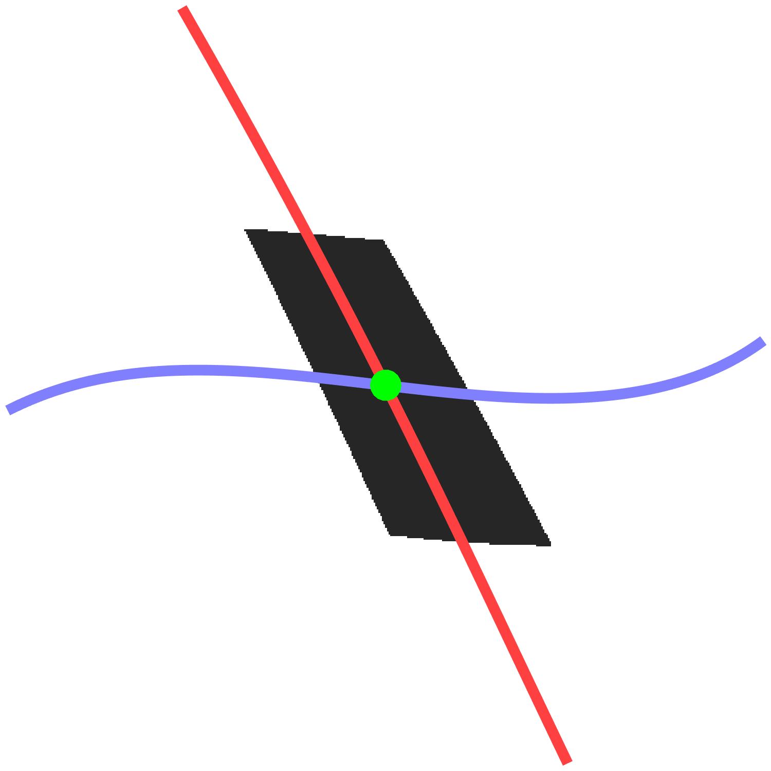
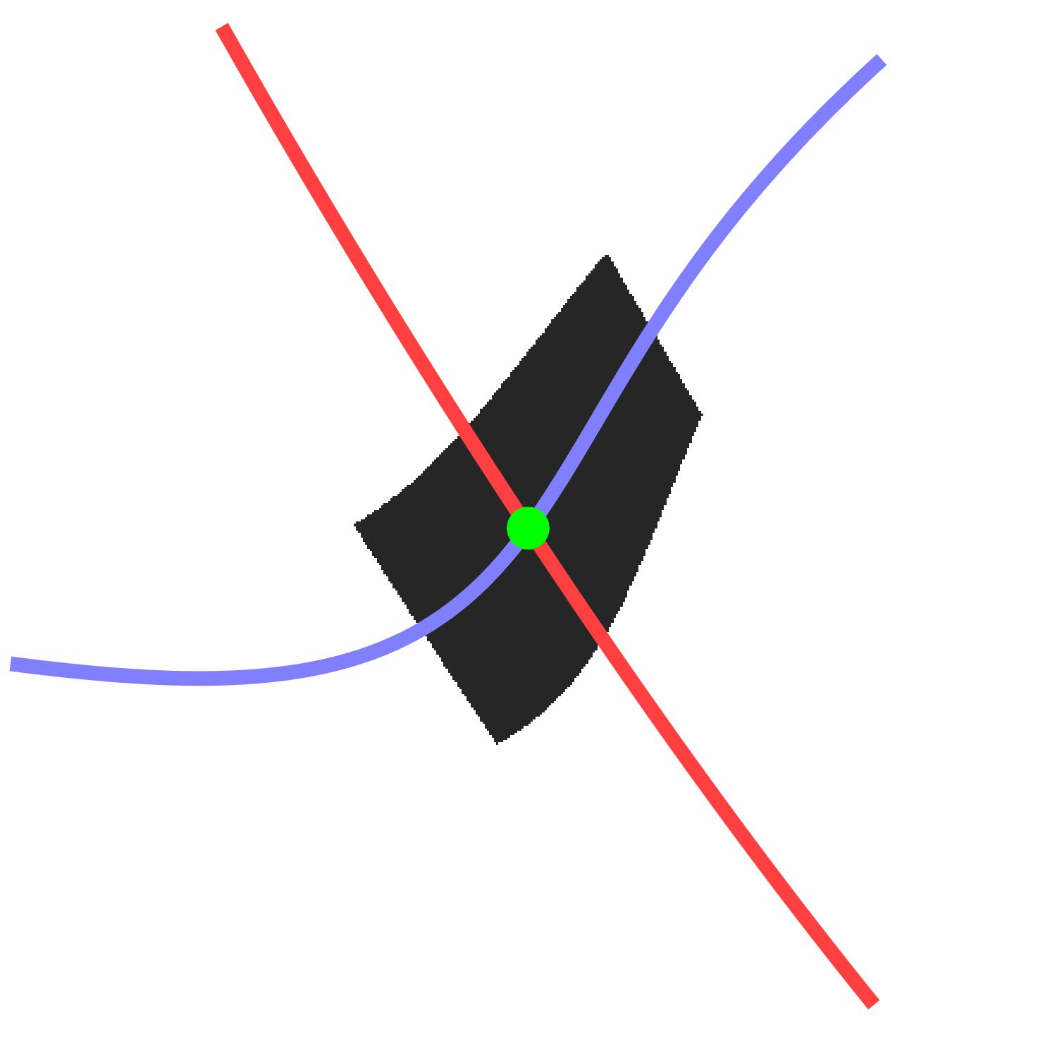
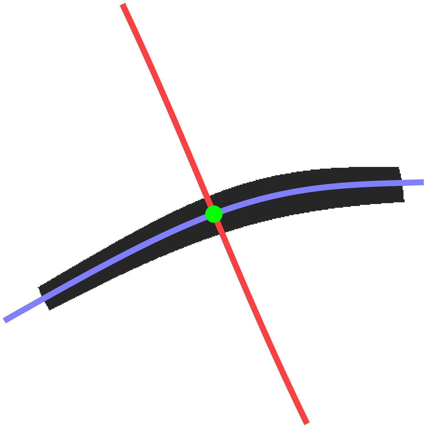
 $t=0$  $t=1$  $t=2$  $t=3$

Figure 2. An illustration of Corollary 2.2 for $T=3$ with the flow direction removed. The green points are $\varphi_{t}(\rho_{0})$, the curves are the local stable (red) and unstable (blue) manifolds of these points, and the black rectangles are the sets $\varphi_{t}(\mathcal{V})$.

Corollary 2.2.

Let $d(\bullet,\bullet)$ and $\varepsilon_{0}>0$ be fixed in Lemma 2.1. Fix $\rho_{0}\in S^{*}M$, $T\in\mathbb{N}_{0}$, and consider the set

$$\mathcal{V}:=\big{\{}\rho\in S^{*}M\mid d(\varphi_{t}(\rho),\varphi_{t}(\rho_{0}))\leq\varepsilon_{0}\quad\text{for all integer}\ t\in[0,T]\big{\}}.$$

Then we have for all $\rho\in\mathcal{V}$ and $t\in[0,T]$

$$d\big{(}\varphi_{t}(\rho),W_{0s}(\varphi_{t}(\rho_{0}))\big{)} \leq C/J^{u}_{T-t}(\rho_{0})\leq Ce^{-\Lambda_{0}(T-t)},$$ (2.27)

$$d\big{(}\varphi_{t}(\rho),W_{0u}(\varphi_{t}(\rho_{0}))\big{)} \leq CJ^{s}_{t}(\varphi_{t}(\rho_{0}))\leq Ce^{-\Lambda_{0}t}.$$

Roughly speaking (2.27) implies that $\varphi_{t}(\mathcal{V})$ lies inside an $\varepsilon_{0}\times e^{-\Lambda_{0}t}\times e^{-\Lambda_{0}(T-t)}$ sized rectangle (with dimensions along $E_{0},E_{s},E_{u}$ respectively) centered at $\varphi_{t}(\rho_{0})$ – see Figure 2.

2.1.2. Straightening out the weak unstable foliation

In §4.3.3 and §4.6.1 below (most crucially in the proof of Lemma 4.15) we rely on the following construction of normal coordinates which straighten out a given weak unstable leaf. Similarly to Lemma 2.1 we fix a distance function $d(\bullet,\bullet)$ on $S^{*}M$.

Lemma 2.3.

For $\varepsilon_{0}>0$ small enough and for any $\rho_{0}\in S^{*}M$ there exists a $C^{\infty}$ symplectomorphism

$$\varkappa=\varkappa_{\rho_{0}}:U_{\rho_{0}}\to V_{\rho_{0}},\quad U_{\rho_{0}}\subset T^{*}M\setminus 0,\quad V_{\rho_{0}}\subset T^{*}\mathbb{R}^{2}\setminus 0,$$

such that, denoting points in $T^{*}M$ by $(x,\xi)$ and points in $T^{*}\mathbb{R}^{2}$ by $(y,\eta)$, we have:

1. $U_{\rho_{0}},V_{\rho_{0}}$ are conic sets and the ball $B_{d}(\rho_{0},\varepsilon_{0})$ is contained in $U_{\rho_{0}}\cap S^{*}M$;

2. $\varkappa$ is homogeneous, namely it maps the vector field $\xi\cdot\partial_{\xi}$ to $\eta\cdot\partial_{\eta}$;

3. $\varkappa(\rho_{0})=(0,0,0,1)$, $d\varkappa(\rho_{0})E_{u}(\rho_{0})=\mathbb{R}\partial_{y_{1}}$, and $d\varkappa(\rho_{0})E_{s}(\rho_{0})=\mathbb{R}\partial_{\eta_{1}}$;

4. putting $p(x,\xi):=|\xi|_{g}$, we have $p=\eta_{2}\circ\varkappa$ on $U_{\rho_{0}}$;

5. for each $\tilde{\rho}\in U_{\rho_{0}}$, the weak unstable leaf $W_{0u}(\tilde{\rho})$ satisfies for some $\tilde{\zeta}=Z(\tilde{\rho})\in\mathbb{R}$

   $$\varkappa(W_{0u}(\tilde{\rho})\cap U_{\rho_{0}})=\big{\{}(y_{1},y_{2},p(\tilde{\rho})F(y_{1},\tilde{\zeta}),p(\tilde{\rho}))\mid(y_{1},\tilde{\zeta})\in\Omega,\ y_{2}\in\mathbb{R}\big{\}}\cap V_{\rho_{0}}$$ (2.28)

   where $F=F_{\rho_{0}}$ is a function from an open set $\Omega=\Omega_{\rho_{0}}\subset\mathbb{R}^{2}$ to $\mathbb{R}$ lying in the Hölder class $C^{3/2}(\Omega)$, the map $y_{1}\mapsto F(y_{1},\zeta)$ is $C^{\infty}$ for every $\zeta$, and $Z:U_{\rho_{0}}\to\mathbb{R}$ is homogeneous of degree 0, in the class $C^{3/2}$ on $U_{\rho_{0}}\cap S^{*}M$, and constant on each local weak unstable leaf;

6. $Z(\rho_{0})=0$, $F(y_{1},0)=0$, and $F(0,\zeta)=\zeta$;

7. $\partial_{\zeta}F(y_{1},0)=1$.

8. there exists $C_{\rho_{0}}>0$ such that $|F(y_{1},\zeta)-\zeta|\leq C_{\rho_{0}}\,|\zeta|^{3/2}$.

The derivatives of all orders of $\varkappa_{\rho_{0}}$ and the constant $C_{\rho_{0}}$ are bounded independently of $\rho_{0}$.

Figure 3. An illustration of Lemma 2.3, restricted to $S^{*}M$ and with the flow direction removed. The curves on the left are the (weak) unstable manifolds and the curves on the right are their images under $\varkappa$.

Remarks. 1. The statements (1)–(7) of Lemma 2.3 rely on the $C^{3/2}$ regularity of the unstable distribution $(E_{u}(\rho))_{\rho\in S^{*}M}$, proved by Hurder–Katok [HK90, Theorem 3.1]. They actually proved that for a generic surface of negative curvature, the distribution has regularity $C^{2-}$, but not better: by [HK90, Theorem 3.2 and Corollary 3.7], if the regularity is $C^{2}$, then $(M,g)$ must have constant curvature. For our application the regularity $C^{1+\epsilon_{0}}$ for some $\epsilon_{0}>0$ would suffice, but we will use the $C^{3/2}$ regularity to simplify the expressions.

2. The point (6) in the Lemma shows that the weak unstable manifold $W_{0u}(\rho_{0})$ is represented, in the coordinates given by $\varkappa$, by the horizontal plane $\{\eta_{1}=0,\,\eta_{2}=1\}$, see (2.29). The nearby unstable leaves $W_{0u}(\tilde{\rho})$ will then be approximately horizontal, that is close to planes $\{\eta_{1}=\zeta=\text{const},\,\eta_{2}=\text{const}\}$. The statements (7)–(8) express this almost horizontality more precisely. In §4 this almost horizontality will allow us to apply the (“straight”) fractal uncertainty principle to families of almost-horizontal unstable manifolds. The statement (8), which relies on the $C^{3/2}$ regularity, will be directly used in Lemma 4.15.

To prove Lemma 2.3 we start by constructing a local coordinate frame under slightly weaker conditions:

Lemma 2.4.

Under the assumptions of Lemma 2.3 there exists a symplectomorphism $\varkappa_{0}$ having properties (1)–(6) of that lemma.

Proof.

To construct $\varkappa_{0}$ we need to define a system of symplectic coordinates $(y_{1},y_{2},\eta_{1},\eta_{2})$ on a conic neighborhood of $\rho_{0}$ which are homogeneous (more precisely $y_{1},y_{2}$ are homogeneous of degree 0 and $\eta_{1},\eta_{2}$ are homogeneous of degree 1). Put $\eta_{2}:=p$ and let $\eta_{1}|_{S^{*}M}$ be a defining function of the leaf $W_{0u}(\rho_{0})$ (namely $\eta_{1}$ vanishes on $W_{0u}(\rho_{0})$ and its differential is nondegenerate on that submanifold) satisfying $H_{p}\eta_{1}=0$; this is possible since $H_{p}$ is tangent to $W_{0u}(\rho_{0})$. Extending $\eta_{1}$ to be homogeneous of degree 1, we see that the Poisson bracket $\{\eta_{1},\eta_{2}\}$ vanishes in a conic neighborhood of $\rho_{0}$. The existence of the system of coordinates $(y_{1},y_{2},\eta_{1},\eta_{2})$ now follows from the Darboux Theorem [HöIII, Theorem 21.1.9], where we can arrange that $y_{1}(\rho_{0})=y_{2}(\rho_{0})=0$.

Since $\varkappa_{0}$ is homogeneous, it sends the canonical 1-form $\xi\,dx$ on $T^{*}M$ to the canonical 1-form $\eta\,dy$ on $T^{*}\mathbb{R}^{2}$. By (2.4) we then have

$$d\varkappa_{0}(\rho_{0})(E_{s}(\rho_{0})\oplus E_{u}(\rho_{0}))=\ker(d\eta_{2})\cap\ker(dy_{2}).$$

Since $E_{u}(\rho_{0})$ is tangent to $W_{0u}(\rho_{0})$, we see that $d\varkappa_{0}(E_{u}(\rho_{0}))=\mathbb{R}\partial_{y_{1}}$. To ensure that $d\varkappa_{0}(E_{s}(\rho_{0}))=\mathbb{R}\partial_{\eta_{1}}$ we compose $\varkappa_{0}$ with the nonlinear shear

$$(y,\eta)\mapsto(y+d\mathcal{F}(\eta),\eta),\quad\mathcal{F}(\eta_{1},\eta_{2}):=\theta{\eta_{1}^{2}\over\eta_{2}}$$

for an appropriate choice of $\theta\in\mathbb{R}$.

Properties (1)–(4) of Lemma 2.3 follow immediately from the discussion above. For property (5), we first note that by construction

$$\varkappa_{0}(W_{0u}(\rho_{0}))=\{\eta_{1}=0,\ \eta_{2}=1\}.$$ (2.29)

Since the tangent spaces $E_{0u}(\rho)$ to the leaves $W_{0u}(\rho)$ depend continuously on $\rho$, we see that for $\tilde{\rho}\in S^{*}M$ near $\rho$ the images $\varkappa_{0}(W_{0u}(\tilde{\rho}))$ project diffeomorphically onto the $(y_{1},y_{2})$ variables. Therefore we can locally write

$$\varkappa_{0}(W_{0u}(\tilde{\rho}))=\{\eta_{1}=F_{0}(y_{1},y_{2},\tilde{\zeta}),\ \eta_{2}=1\}$$

for some function $F_{0}(y_{1},y_{2},\zeta)$ and some $\tilde{\zeta}=Z_{0}(\tilde{\rho})$ depending on $\tilde{\rho}$, and we can assume that $F_{0}(0,0,\zeta)=\zeta$ which uniquely determines the functions $F_{0},Z_{0}$. Since $W_{0u}(\tilde{\rho})$ is a $C^{\infty}$ submanifold, the function $y\mapsto F_{0}(y,\zeta)$ is $C^{\infty}$ for each $\zeta$. Since $H_{p}$ is tangent to each $W_{0u}(\tilde{\rho})$ and is mapped by $\varkappa_{0}$ to $\partial_{y_{2}}$, we see that $\partial_{y_{2}}F_{0}=0$, thus $F_{0}$ is a function of $(y_{1},\zeta)$ only. This shows that (2.28) holds for all $\tilde{\rho}\in U_{\rho_{0}}\cap S^{*}M$, and it is easy to see that it holds for all $\tilde{\rho}\in U_{\rho_{0}}$ by homogeneity, with $Z_{0}$ homogeneous of degree 0. Property (6) follows from (2.29).

It remains to prove that the functions $F_{0},Z_{0}$ have regularity $C^{3/2}$. According to [HK90, Definition 4.1 and Theorem 4.2], the function $F_{0}$ is $C^{\infty}$ in the variable $y_{1}$ (this shows that each unstable leaf is smooth submanifold), and is $C^{1}$ w.r.t. $\zeta$. Besides, [HK90, Theorem 3.1] shows that the distribution $E_{u}(\rho)$ depends $C^{3/2}$ on $\rho$. In our coordinates $\varkappa_{0}$, this regularity means that the “slope function” $e_{u}(y_{1},\eta_{1})$ of the unstable distribution has regularity $C^{3/2}$ w.r.t. its variables. Now, the function $F_{0}$ is a solution of the differential equation

$$\frac{d}{dy_{1}}F_{0}(y_{1},\zeta)=e_{u}\big{(}y_{1},F_{0}(y_{1},\zeta)\big{)},\quad\text{with initial condition}\ \ F_{0}(0,\zeta)=\zeta.$$

Standard results on ODEs [Ha02, Chapter V] show that the unique solution to such an ODE with $C^{k}$ function $e_{u}$ will depend in a $C^{k}$ way of the initial condition $\zeta$. The proof of [Ha02, Theorem 3.1] can be easily adapted to show that a $C^{3/2}$ function $e_{u}$ induces a solution $F_{0}$ with regularity $C^{3/2}$. ∎

We now modify the map $\varkappa_{0}$ from Lemma 2.4 to obtain a map $\varkappa$ satisfying also the condition (7) of Lemma 2.3. Let $F_{0}$ be the function constructed in the proof of Lemma 2.4. We have for every $\zeta$

$$y_{1}\mapsto\partial_{\zeta}F_{0}(y_{1},\zeta)\quad\text{lies in }C^{\infty}.$$ (2.30)

This follows from the existence of $C^{\infty}$-adapted transverse coordinates, see [HK90, Point 2 in Definition 4.1 and Proposition 4.2].

From the normalization $F_{0}(0,\zeta)=\zeta$ we see that $\partial_{\zeta}F_{0}(y_{1},\zeta)>0$ for $y_{1}$ close to 0. Take the diffeomorphism $\psi$ of neighborhoods of $0$ in $\mathbb{R}$ defined by

$$\psi(y_{1})=\int_{0}^{y_{1}}\partial_{\zeta}F_{0}(s,0)\,ds.$$

We define $\varkappa$ as the composition $\varkappa:=\Psi\circ\varkappa_{0}$ where $\Psi$ is the symplectic lift of $\psi$:

$$\Psi(y_{1},y_{2},\eta_{1},\eta_{2})=(\psi(y_{1}),y_{2},\eta_{1}/\psi^{\prime}(y_{1}),\eta_{2}).$$

Then $\varkappa$ satisfies all the properties in Lemma 2.3, with the function

$$F(y_{1},\zeta)={F_{0}(\psi^{-1}(y_{1}),\zeta)\over\partial_{\zeta}F_{0}(\psi^{-1}(y_{1}),0)},\quad Z=Z_{0}\,.$$

Like $F_{0}$, the function $F$ is $C^{3/2}$ w.r.t. the variable $\zeta$. We now use this regularity to prove part (8) of Lemma 2.3. This $C^{3/2}$ regularity, together with the property (7), implies the Taylor expansion of $F$ at the point $(y_{1},0)$:

$$F(y_{1},\zeta) =F(y_{1},0)+\zeta\partial_{\zeta}F(y_{1},0)+\mathcal{O}(\zeta^{3/2})$$

$$=\zeta+\mathcal{O}(\zeta^{3/2}),$$

with the implied constant being uniform w.r.t. $y_{1}$. The second line is the point (8) of the Lemma: the leaf $W_{0u}(\rho)$ at “height” $\zeta$ from the reference horizontal leaf $W_{0u}(\rho_{0})$ is contained in horizontal rectangle of thickness $\mathcal{O}(\zeta^{3/2})$.

Finally, the fact that the derivatives of all orders of $\varkappa_{\rho_{0}}$ are bounded uniformly in $\rho_{0}$ follows directly from the arguments above and the fact that the leaf $W_{0u}(\rho_{0})$ depends continuously on $\rho_{0}$ as an embedded $C^{\infty}$ submanifold of $S^{*}M$. It also shows that the constant $C_{\rho_{0}}$ in item (8) is uniformly bounded w.r.t $\rho_{0}$. $\square$

2.2. Pseudodifferential operators

Let $M$ be a manifold. We use the standard semiclassical symbol class $S^{k}_{h}(T^{*}M)$ whose elements $a(x,\xi;h)$ satisfy uniform derivative bounds on every compact subset $K\subset M$:

$$|\partial^{\alpha}_{x}\partial^{\beta}_{\xi}a(x,\xi;h)|\leq C_{\alpha\beta K}\langle\xi\rangle^{k-|\beta|},\quad x\in K,\ \xi\in T^{*}_{x}M,$$

and admit an expansion in powers of $h$ and $|\xi|$. See for instance [DZ19, Definition E.3] or [DZ16, §2.1]. Denote by $S^{k}(T^{*}M)$ the class of $h$-independent symbols in $S^{k}_{h}(T^{*}M)$. We fix a (noncanonical) quantization procedure $\operatorname{Op}_{h}$ on $M$, see (A.5) below and [DZ19, Proposition E.15]. Denote the class of semiclassical pseudodifferential operators with symbols in $S^{k}_{h}(T^{*}M)$ by $\Psi^{k}_{h}(M)$ and the (canonical) principal symbol map by $\sigma_{h}:\Psi^{k}_{h}(M)\to S^{k}(T^{*}M)$. See for instance [DZ19, §E.1.7] or [Zw12, §14.2].

If $M$ is noncompact, then we do not impose any restrictions on the growth of $a(x,\xi;h)\in S^{k}_{h}(T^{*}M)$ as $|x|\to\infty$ and likewise do not say anything about the asymptotic behavior of operators in $\Psi^{k}_{h}(M)$ as we approach the infinity of $M$. Therefore in general operators in $\Psi^{k}_{h}(M)$ are bounded (uniformly in $h$) acting $H^{s}_{h,\operatorname{comp}}(M)\to H^{s-k}_{h,\operatorname{loc}}(M)$ where $H^{s}_{h,\operatorname{loc}}(M)$ denotes the space of distributions locally in the semiclassical Sobolev space $H^{s}_{h}$ and $H^{s}_{h,\operatorname{comp}}(M)$ consists of the compactly supported elements of $H^{s}_{h,\operatorname{loc}}(M)$. See [DZ19, §E.1.8] or [Zw12, §8.3.1]. We will typically use operators in $\Psi^{k}_{h}(M)$ which are properly supported, mapping $H^{s}_{h,\operatorname{comp}}(M)\to H^{s-k}_{h,\operatorname{comp}}(M)$ and $H^{s}_{h,\operatorname{loc}}(M)\to H^{s-k}_{h,\operatorname{loc}}(M)$. The quantization procedure $\operatorname{Op}_{h}$ is chosen so that $\operatorname{Op}_{h}(a)$ is properly supported for every $a$ and $\operatorname{Op}_{h}(a)$ is compactly supported (i.e. it has a compactly supported Schwartz kernel) for symbols $a$ which are compactly supported in the $x$ variable. Of course if $M$ is a compact manifold (which will mostly be the case in this paper), then $H^{s}_{h,\operatorname{loc}}(M)$ and $H^{s}_{h,\operatorname{comp}}(M)$ are the same space, denoted by $H^{s}_{h}(M)$. We will mostly use the space $H^{0}_{h}(M)=L^{2}(M)$.

For $A\in\Psi^{k}_{h}(M)$ we denote by $\operatorname{WF}_{h}(A)$ its wavefront set and by $\operatorname{ell}_{h}(A)$ its elliptic set. Both are subsets of the fiber-radially compactified cotangent bundle $\overline{T}^{*}M$. See for instance [DZ19, §E.2] or [DZ16, §2.1]. For $A\in\Psi^{k}_{h}(M)$, $B\in\Psi^{\ell}_{h}(M)$ we say that

$$A=B+\mathcal{O}(h^{\infty})\quad\text{microlocally on some open set $U\subset\overline{T}^{*}M$}$$

if $\operatorname{WF}_{h}(A-B)\cap U=\emptyset$.

We also use the notion of the wavefront set $\operatorname{WF}_{h}(u)\subset\overline{T}^{*}M$ of an $h$-dependent tempered family of distributions $u=u(h)\in\mathcal{D}^{\prime}(M)$ and the wavefront set $\operatorname{WF}_{h}^{\prime}(B)\subset\overline{T}^{*}(M_{1}\times M_{2})$ of an $h$-dependent tempered family of operators $B=B(h):C^{\infty}_{\mathrm{c}}(M_{2})\to\mathcal{D}^{\prime}(M_{1})$, see [DZ19, §E.2.3].

2.2.1. Mildly exotic symbols

We also use the mildly exotic symbol class $S^{\operatorname{comp}}_{\delta}(T^{*}M)$, $\delta\in[0,{1\over 2})$, consisting of symbols $a(x,\xi;h)$ such that:

• the $(x,\xi)$-support of $a$ is contained in an $h$-independent compact subset of $T^{*}M$;

• the symbol $a$ satisfies derivative bounds

  $$|\partial^{\alpha}_{(x,\xi)}a(x,\xi;h)|\leq C_{\alpha\beta}h^{-\delta|\alpha|}.$$

The operator class corresponding to $S^{\operatorname{comp}}_{\delta}(T^{*}M)$ is denoted by $\Psi_{\delta}^{\operatorname{comp}}(M)$. We require operators in $\Psi_{\delta}^{\operatorname{comp}}(M)$ to be compactly supported. We use the same quantization procedure $\operatorname{Op}_{h}$ for this class and note that compactly supported elements of $S^{k}_{h}(T^{*}M)$ lie in $S^{\operatorname{comp}}_{0}(T^{*}M)$. See [Zw12, §4.4] or [DG14, §3.1].

Operators in the class $\Psi^{\operatorname{comp}}_{\delta}(M)$ satisfy the following version of the sharp Gårding inequality for all $u\in L^{2}(M)$:

$$a\in S^{\operatorname{comp}}_{\delta}(T^{*}M),\ \operatorname{Re}a\geq 0\quad\Longrightarrow\quad\operatorname{Re}\langle\operatorname{Op}_{h}(a)u,u\rangle_{L^{2}}\geq-Ch^{1-2\delta}\|u\|_{L^{2}}^{2}$$ (2.31)

where the constant $C$ depends only on a certain $S^{\operatorname{comp}}_{\delta}(T^{*}M)$ seminorm of $a$. The inequality (2.31) can be reduced to the case of the standard quantization on $\mathbb{R}^{n}$; the latter case is proved by applying the standard sharp Gårding inequality [Zw12, Theorem 4.32] to the rescaled symbol $\tilde{a}(x,\xi):=a(h^{\delta}x,h^{\delta}\xi)$ and using the identity $\operatorname{Op}_{h}(a)=T^{-1}\operatorname{Op}_{h^{1-2\delta}}(\tilde{a})T$ where $Tu(x)=u(h^{\delta}x)$.

We also have the following norm bound when $M$ is compact:

$$a\in S^{\operatorname{comp}}_{\delta}(T^{*}M)\quad\Longrightarrow\quad\|\operatorname{Op}_{h}(a)\|_{L^{2}\to L^{2}}\leq\sup_{T^{*}M}|a|+Ch^{{1\over 2}-\delta}$$ (2.32)

where the constant $C$ depends only on some $S^{\operatorname{comp}}_{\delta}(T^{*}M)$ seminorm of $a$. To show (2.32) it suffices to apply (2.31) to the operator $c^{2}-\operatorname{Op}_{h}(a)^{*}\operatorname{Op}_{h}(a)=\operatorname{Op}_{h}(c^{2}-|a|^{2})+\mathcal{O}(h^{1-2\delta})_{L^{2}\to L^{2}}$ where $c=c(h):=\sup_{T^{*}M}|a|$.

Notation: We remark that there is a slight conflict of notation between the classes $S^{k}_{h}$ ($h$-dependent symbols of order $k$ in $\xi$ which are polyhomogeneous in both $\xi$ and $h$) and $S^{\operatorname{comp}}_{\delta}$ ($h$-dependent compactly supported symbols losing $h^{-\delta}$ with each differentiation). A more proper notation would be

$$S^{k}_{h,\text{phg}}(T^{*}M):=S^{k}_{h}(T^{*}M),\quad S^{\operatorname{comp}}_{h,\delta}(T^{*}M):=S^{\operatorname{comp}}_{\delta}(T^{*}M).$$

We however keep the shorter notation to reduce the number of indices used. For $\delta\in[0,{1\over 2})$ we define the symbol class

$$S^{\operatorname{comp}}_{\delta+}(T^{*}M)=\bigcap_{\epsilon>0}S^{\operatorname{comp}}_{\delta+\epsilon}(T^{*}M).$$

We also use the following notation:

$$f(h)=\mathcal{O}(h^{\alpha-})\quad\text{if}\quad f(h)=\mathcal{O}_{\epsilon}(h^{\alpha-\epsilon})\quad\text{for all }\epsilon>0.$$

When writing $a\in C^{\infty}_{\mathrm{c}}(T^{*}M)$ for a symbol $a$, we assume that $a$ is $h$-independent unless stated otherwise.

2.2.2. Egorov’s Theorem

We now specialize to the case when $(M,g)$ is a compact Anosov surface as in §2.1. Since $\sigma_{h}(-h^{2}\Delta)=p^{2}$ where $p(x,\xi)=|\xi|_{g}$, by the functional calculus of pseudodifferential operators (see [Zw12, Theorem 14.9] or [DS99, §8]) we have

$$\begin{gathered}\psi\in C^{\infty}_{\mathrm{c}}(\mathbb{R})\quad\Longrightarrow\quad\psi(-h^{2}\Delta)\in\Psi^{-\infty}_{h}(M),\\ \operatorname{WF}_{h}(\psi(-h^{2}\Delta))\subset\operatorname{supp}\psi(p^{2}),\quad\sigma_{h}(\psi(-h^{2}\Delta))=\psi(p^{2}).\end{gathered}$$ (2.33)

We now discuss conjugation of pseudodifferential operators by the wave group. Similarly to [DJ18, §2.2], to avoid technical issues coming from the zero section, instead of the true half-wave propagator $e^{-it\sqrt{-\Delta}}$ we use the unitary operator

$$U(t):=\exp(-itP/h),\quad P:=\psi_{P}(-h^{2}\Delta)\in\Psi^{-\infty}_{h}(M),\quad P^{*}=P,$$ (2.34)

where we fixed some function

$$\psi_{P}\in C^{\infty}_{\mathrm{c}}((0,\infty);\mathbb{R}),\quad\operatorname{supp}\psi_{P}\subset\{\textstyle{1\over 25}<\lambda<25\},\quad\psi_{P}(\lambda)=\sqrt{\lambda}\quad\text{for }{\textstyle{1\over 16}\leq\lambda\leq 16}.$$

For a bounded operator $A$ on $L^{2}(M)$, we define the Heisenberg-evolved operators

$$A(t):=U(-t)AU(t),\qquad t\in\mathbb{R}\,.$$ (2.35)

Assume that $a\in C^{\infty}_{\mathrm{c}}(T^{*}M)$ and $\operatorname{supp}a\subset\{{1\over 4}<|\xi|_{g}<4\}$. Then Egorov’s Theorem [Zw12, Theorem 11.1] implies that for $t$ bounded independently of $h$ we have

$$A=\operatorname{Op}_{h}(a)\quad\Longrightarrow\quad A(t)=\operatorname{Op}_{h}(a\circ\varphi_{t})+\mathcal{O}(h)_{L^{2}\to L^{2}}$$ (2.36)

where $\varphi_{t}=\exp(tH_{p})$ is the homogeneous geodesic flow. In fact, the proof in [Zw12] gives the following stronger statement (see e.g. [DG14, §C.2] or Lemma A.7 below for details): for each time $t$ there exists $a_{t}(x,\xi;h)\in S^{\operatorname{comp}}_{0}(T^{*}M)$ such that

$$A(t)=\operatorname{Op}_{h}(a_{t})+\mathcal{O}(h^{\infty})_{\Psi^{-\infty}},\quad a_{t}=a\circ\varphi_{t}+\mathcal{O}(h),\quad\operatorname{supp}a_{t}\subset\varphi_{-t}(\operatorname{supp}a).$$ (2.37)

We next extend (2.36) to the case of $t$ bounded by a small constant times $\log(1/h)$, using the mildly exotic symbol classes described in §2.2.1. Let $\Lambda_{1}>0$ be the ‘maximal expansion rate’ from (2.10). It follows from (2.7) and (2.10) that

$$\sup_{\rho\in\{{1\over 4}\leq|\xi|_{g}\leq 4\}}\|d\varphi_{t}(\rho)\|\leq Ce^{\Lambda_{1}|t|}\quad\text{for all }t\in\mathbb{R}.$$ (2.38)

Lemma 2.5.

Assume that $a\in C^{\infty}_{\mathrm{c}}(T^{*}M)$ and $\operatorname{supp}a\subset\{{1\over 4}\leq|\xi|_{g}\leq 4\}$; put $A:=\operatorname{Op}_{h}(a)$. Fix $\delta\in(0,{1\over 2})$. Then we have uniformly in $t$ satisfying $|t|\leq\delta\Lambda_{1}^{-1}\log(1/h)$:

1. $a\circ\varphi_{t}\in S^{\operatorname{comp}}_{\delta+}(T^{*}M)$;

2. $A(t)=\operatorname{Op}_{h}(a\circ\varphi_{t})+\mathcal{O}(h^{1-2\delta-})_{L^{2}\to L^{2}}$.

Remarks. 1. A stronger statement similar to (2.37), which shows that the remainder $\mathcal{O}(h^{1-2\delta-})$ is actually pseudodifferential, is proved for instance in [DG14, Proposition 3.9].

2. Lemma 2.5 shows that Egorov’s theorem holds for all times $t$ which are smaller (by at least $\epsilon\log(1/h)$ for some $\epsilon>0$) than the minimal Ehrenfest time $\log(1/h)\over 2\Lambda_{1}$. Later we will show a finer version of Egorov’s theorem, up to the (potentially much longer) local Ehrenfest time – see Proposition 4.2.

Proof.

(1) The estimate (2.38) implies the following bounds on higher derivatives: for all $t\in\mathbb{R}$, all multiindices $\alpha$, and all $\epsilon>0$

$$\sup_{T^{*}M}|\partial^{\alpha}(a\circ\varphi_{t})|\leq C_{\alpha,\epsilon}e^{(\Lambda_{1}+\epsilon)|\alpha|\cdot|t|}.$$ (2.39)

See for instance [DG14, Lemma C.1], whose proof applies directly to the present situation; alternatively one could use the proof of Lemma 5.2 below in the special case $k=0$. Under the condition $|t|\leq\delta\Lambda_{1}^{-1}\log(1/h)$ the bound (2.39) implies that $a\circ\varphi_{t}\in S^{\operatorname{comp}}_{\delta+}(T^{*}M)$ uniformly in $t$.

(2) We use the following commutator formula valid for all $\tilde{a}\in S^{\operatorname{comp}}_{\delta+}(T^{*}M)$ with $\operatorname{supp}\tilde{a}\subset\{{1\over 4}\leq|\xi|_{g}\leq 4\}$:

$$[P,\operatorname{Op}_{h}(\tilde{a})]=-ih\operatorname{Op}_{h}(H_{p}\tilde{a})+\mathcal{O}(h^{2-2\delta-})_{L^{2}\to L^{2}}.$$ (2.40)

Here it is important that $p\in S^{\operatorname{comp}}_{0}(T^{*}M)$ and we use the same quantization procedure $\operatorname{Op}_{h}$ on both sides of the equation; the $S^{\operatorname{comp}}_{\delta}$ calculus would only give an $\mathcal{O}(h^{2-4\delta-})$ remainder. See Remark 2 following Lemma A.6 for the proof.

Using (2.40) and part (1) we compute for $|t|\leq\delta\Lambda_{1}^{-1}\log(1/h)$

$$\partial_{t}\big{(}U(t)\operatorname{Op}_{h}(a\circ\varphi_{t})U(-t)\big{)} =U(t)\big{(}-ih^{-1}[P,\operatorname{Op}_{h}(a\circ\varphi_{t})]+\operatorname{Op}_{h}(\partial_{t}(a\circ\varphi_{t}))\big{)}U(-t)$$

$$=\mathcal{O}(h^{1-2\delta-})_{L^{2}\to L^{2}}.$$

Integrating this from 0 to $t$, we get $U(t)\operatorname{Op}_{h}(a\circ\varphi_{t})U(-t)=\operatorname{Op}_{h}(a)+\mathcal{O}(h^{1-2\delta-})_{L^{2}\to L^{2}}$ which finishes the proof since $U(t)$ is unitary. ∎

We will also need to control products of many pseudodifferential operators. The following Lemma considers products of logarithmically many pseudodifferential operators; it is proved in the same way as [DJ18, Lemmas A.1 and A.6] using the norm bound (2.32):

Lemma 2.6.

Let $C$ be an arbitrary fixed constant, $\delta\in[0,{1\over 2})$, and assume that the symbols

$$a_{1},\dots,a_{N}\in S^{\operatorname{comp}}_{\delta}(T^{*}M),\quad N\leq C\log(1/h),\quad\sup|a_{j}|\leq 1$$

have each $S^{\operatorname{comp}}_{\delta}$ seminorm bounded uniformly in $j$. Assume also that we are given operators $A_{j}=\operatorname{Op}_{h}(a_{j})+\mathcal{O}(h^{1-2\delta})_{L^{2}\to L^{2}}$ with the remainders bounded uniformly in $j$. Then:

1. $a_{1}\cdots a_{N}\in S^{\operatorname{comp}}_{\delta+}(T^{*}M)$;

2. $A_{1}\cdots A_{N}=\operatorname{Op}_{h}(a_{1}\cdots a_{N})+\mathcal{O}(h^{1-2\delta-})_{L^{2}\to L^{2}}$.

That is, the product of these symbols (resp. operators) is essentially in the same symbol class (resp. operator class) as the individual factors.

2.3. Lagrangian distributions and Fourier integral operators

In this section we review the theory of semiclassical Lagrangian distributions and Fourier integral operators. These are used in §4.3.3 to describe propagation of Lagrangian states beyond the Ehrenfest time. In particular we use that the wave propagator $U(t)$ defined in (2.34) is, after appropriate cutoffs, a Fourier integral operator associated to the geodesic flow $\varphi_{t}$, see (4.47). Fourier integral operators are also used in §4.6.4 to quantize a symplectomorphism which locally straightens out unstable leaves.

We keep the presentation brief, referring the reader to [Al08], [GS77, Chapter 5], and [GS13, Chapter 8] for details. For other reviews (bearing some similarities to the one here) see [DD13, §3.2], [DG14, §3.2], [Dy15, §3.2], [DZ16, §2.2], and [NZ09, §4.1]. For the related nonsemiclassical case, see [HöIV, Chapter 25] and [GS94, Chapters 10–11].

2.3.1. Lagrangian manifolds and phase functions

Let $M$ be a smooth $n$-dimensional manifold (in this subsection we do not assume $M$ to be compact). Denote by $\xi\,dx$ the canonical 1-form on $T^{*}M$, then the symplectic form is given by

$$\omega:=d(\xi\,dx).$$

An embedded $n$-dimensional submanifold $\mathscr{L}\subset T^{*}M$ is called a Lagrangian submanifold if the pullback of $\omega$ to $\mathscr{L}$ is zero; that is, the pullback of $\xi\,dx$ to $\mathscr{L}$ is a closed 1-form. A Lagrangian submanifold is called exact if the pullback of $\xi\,dx$ to $\mathscr{L}$ is equal to $dF$ for some function $F\in C^{\infty}(\mathscr{L};\mathbb{R})$, called an antiderivative on $\mathscr{L}$. We henceforth define an exact Lagrangian submanifold as the pair $(\mathscr{L},F)$ but still often denote it by $\mathscr{L}$ for simplicity.

We note that $\mathscr{L}$ is exact in particular if it is conic, namely the generator of dilations $\xi\cdot\partial_{\xi}$ is tangent to $\mathscr{L}$. In this case the pullback of $\xi\,dx$ to $\mathscr{L}$ is equal to 0 (since $\omega(\xi\cdot\partial_{\xi},v)=\langle\xi\,dx,v\rangle=0$ for any tangent vector $v\in T\mathscr{L}$), thus it is natural to fix the antiderivative equal to 0 as well.

One way to obtain an exact Lagrangian submanifold is by using a phase function. More precisely, if $U\subset M_{x}\times\mathbb{R}^{m}_{\theta}$ is an open set (for some $m\in\mathbb{N}_{0}$) then we call a function $\Phi(x,\theta)\in C^{\infty}(U;\mathbb{R})$ a nondegenerate phase function if:

1. the differentials $d(\partial_{\theta_{j}}\Phi)_{1\leq j\leq m}$ are linearly independent on the critical set

   $$\mathcal{C}_{\Phi}:=\{(x,\theta)\in U\mid\partial_{\theta}\Phi(x,\theta)=0\}$$

   which is then an $n$-dimensional embedded submanifold of $U$; and

2. the following map is a smooth embedding:

   $$j_{\Phi}:\mathcal{C}_{\Phi}\to T^{*}M,\quad j_{\Phi}(x,\theta)=(x,\partial_{x}\Phi(x,\theta)).$$

We call $\theta$ the oscillatory variables.

Under the conditions (1)–(2) above the manifold

$$\mathscr{L}_{\Phi}:=j_{\Phi}(\mathcal{C}_{\Phi})\ \subset\ T^{*}M$$ (2.41)

is exact Lagrangian, with the antiderivative $F_{\Phi}\in C^{\infty}(\mathscr{L}_{\Phi};\mathbb{R})$ given by the restriction of the phase function on the critical set:

$$F_{\Phi}(j_{\Phi}(x,\theta))=\Phi(x,\theta),\quad(x,\theta)\in\mathcal{C}_{\Phi}.$$

For an exact Lagrangian submanifold $(\mathscr{L},F)$ we say that a nondegenerate phase function $\Phi$ generates $\mathscr{L}$, if $\mathscr{L}=\mathscr{L}_{\Phi}$ and $F=F_{\Phi}$.

Every exact Lagrangian submanifold $(\mathscr{L},F)$ is locally generated by phase functions: that is, each point $\rho\in\mathscr{L}$ has a neighborhood generated by some phase function; see [GS77, Proposition 5.1]. The simplest case is when the projection $\pi:\mathscr{L}\to M$ is a diffeomorphism onto its image, in which case $\mathscr{L}$ is given by

$$\mathscr{L}=\mathscr{L}_{\Phi}=\{(x,\partial_{x}\Phi(x))\mid x\in U\},\quad U:=\pi(\mathscr{L})\subset M,$$ (2.42)

where the function $\Phi\in C^{\infty}(U;\mathbb{R})$ is defined by $F(x,\xi)=\Phi(x)$ for all $(x,\xi)\in\mathscr{L}$.

Another important case is when $\mathscr{L}\subset T^{*}M\setminus 0$ is conic. In this case each point $\rho\in\mathscr{L}$ has a conic neighborhood which is generated by some phase function $\Phi(x,\theta)$, $(x,\theta)\in U$, where $U\subset M\times\mathbb{R}^{m}$ is conic and $\Phi$ is homogeneous of degree 1 in the $\theta$ variables. For the proof see [GS77, Proposition 5.2], [HöIII, Theorem 21.2.16], or [GS94, Proposition 11.4].

2.3.2. Lagrangian distributions

Let $(\mathscr{L},F)$ be an exact Lagrangian submanifold of $T^{*}M$. We use the class $I^{\operatorname{comp}}_{h}(\mathscr{L})$ of (compactly microlocalized semiclassical) Lagrangian distributions associated to $\mathscr{L}$. Elements of $I^{\operatorname{comp}}_{h}(\mathscr{L})$ are $h$-dependent families of functions in $C^{\infty}_{\mathrm{c}}(M)$, with support contained in some $h$-independent compact set. We give a definition and some properties of the class $I^{\operatorname{comp}}_{h}(\mathscr{L})$ below.

If $\mathscr{L}=\mathscr{L}_{\Phi}$ is generated by some phase function $\Phi(x,\theta)$, $(x,\theta)\in U\subset M\times\mathbb{R}^{m}$, in the sense of (2.41), then $I^{\operatorname{comp}}_{h}(\mathscr{L})$ consists of distributions of the form

$$u(x;h)=(2\pi h)^{-m/2}\int_{\mathbb{R}^{m}}e^{i\Phi(x,\theta)/h}a(x,\theta;h)\,d\theta+\mathcal{O}(h^{\infty})_{C^{\infty}_{\mathrm{c}}(M)}.$$ (2.43)

Here the amplitude $a(x,\theta;h)\in C^{\infty}_{\mathrm{c}}(U)$ is a classical symbol; that is, $\operatorname{supp}a$ is contained in an $h$-independent compact subset of $U$ and we have the asymptotic expansion in $C^{\infty}_{\mathrm{c}}(U)$

$$a(x,\theta;h)\sim\sum_{j=0}^{\infty}h^{j}a_{j}(x,\theta)\quad\text{as}\quad h\to 0$$

for some $a_{0},a_{1},\ldots\in C^{\infty}_{\mathrm{c}}(U)$.

In the special case when $\Phi$ has no oscillatory variables (i.e. $\mathscr{L}$ is given by (2.42)) the expression (2.43) simplifies to

$$u(x;h)=e^{i\Phi(x)/h}a(x;h)+\mathcal{O}(h^{\infty})_{C^{\infty}_{\mathrm{c}}(M)}.$$ (2.44)

The class of functions defined by (2.43) does not depend on the choice of the phase function generating $\mathscr{L}$. That is, if $\Phi,\Phi^{\prime}$ are two phase functions with $\mathscr{L}=\mathscr{L}_{\Phi}=\mathscr{L}_{\Phi^{\prime}}$ and $u$ is given by (2.43) for the phase function $\Phi$ and some amplitude $a$, then $u$ is also given by (2.43) for the phase function $\Phi^{\prime}$ and some other amplitude $a^{\prime}$. The simplest case of this statement is when $\Phi^{\prime}$ has no oscillatory variables (that is, $\mathscr{L}$ is constructed from $\Phi^{\prime}$ using (2.42)) as we can then write (ignoring the $\mathcal{O}(h^{\infty})$ remainder in (2.43))

$$a^{\prime}(x;h)=e^{-i\Phi^{\prime}(x)/h}u(x;h)=(2\pi h)^{-m/2}\int_{\mathbb{R}^{m}}e^{{i\over h}(\Phi(x,\theta)-\Phi^{\prime}(x))}a(x,\theta;h)\,d\theta$$ (2.45)

and show that $a^{\prime}$ is a classical symbol using the method of stationary phase. The proof in the general case also uses stationary phase but is more involved, see [GS13, §8.1.2]; for the nonsemiclassical case see [GS77, §6.4], [HöIV, Proposition 25.1.5], or [GS94, Theorem 11.5].

For general Lagrangians $\mathscr{L}$ (not parametrized by a single phase function) we define $I^{\operatorname{comp}}_{h}(\mathscr{L})$ as consisting of sums $u_{1}+\dots+u_{k}$ where $u_{j}\in I^{\operatorname{comp}}_{h}(\mathscr{L}_{j})$ and each $\mathscr{L}_{j}\subset\mathscr{L}$ is generated by some phase function. Here are two important properties of Lagrangian distributions:

1. If $u\in I^{\operatorname{comp}}_{h}(\mathscr{L})$ and $A\in\Psi^{k}_{h}(M)$ is compactly supported (which means that its Schwartz kernel is compactly supported) then $Au\in I^{\operatorname{comp}}_{h}(\mathscr{L})$;

2. If $u\in I^{\operatorname{comp}}_{h}(\mathscr{L})$ then $\operatorname{WF}_{h}(u)\subset\mathscr{L}$; that is, for any compactly supported $A\in\Psi^{k}_{h}(M)$ with $\operatorname{WF}_{h}(A)\cap\mathscr{L}=\emptyset$ we have $Au=\mathcal{O}(h^{\infty})_{C^{\infty}_{\mathrm{c}}(M)}$.

To show these, we first use a partition of unity to reduce to the case when $M=\mathbb{R}^{n}$ and $\mathscr{L}$ is generated by some phase function $\Phi$. We next write for $b\in C^{\infty}_{\mathrm{c}}(T^{*}\mathbb{R}^{n})$ and $u$ given by (2.43)

$$\operatorname{Op}_{h}(b)u(x)=(2\pi h)^{-{m\over 2}-n}\int_{\mathbb{R}^{2n+m}}e^{{i\over h}(\langle x-y,\xi\rangle+\Phi(y,\theta))}b(x,\xi)a(y,\theta;h)\,dyd\xi d\theta.$$

We now apply stationary phase in the $(y,\xi)$ variables to get an expression of the form (2.43) with the phase function $\Phi(x,\theta)$ and some amplitude which is a classical symbol. On the other hand, if $b$ is a symbol in $S^{k}_{h}(T^{*}\mathbb{R}^{n})$ and $\operatorname{supp}b\cap\mathscr{L}=\emptyset$ then the method of nonstationary phase in the $(y,\xi,\theta)$ variables shows that $\operatorname{Op}_{h}(b)u(x)=\mathcal{O}(h^{\infty})_{C^{\infty}}$.

2.3.3. Fourier integral operators

We next discuss Fourier integral operators associated to symplectomorphisms. Let $M_{1},M_{2}$ be two manifolds of the same dimension $n$, $U_{j}\subset T^{*}M_{j}$ be two open sets, and $\varkappa:U_{2}\to U_{1}$ be a symplectomorphism. The flipped graph

$$\mathscr{L}_{\varkappa}:=\{(x_{1},\xi_{1},x_{2},-\xi_{2})\mid(x_{2},\xi_{2})\in U_{2},\ \varkappa(x_{2},\xi_{2})=(x_{1},\xi_{1})\}\subset T^{*}(M_{1}\times M_{2})$$ (2.46)

is a Lagrangian submanifold. We further assume that $\varkappa$ is exact, namely $\mathscr{L}_{\varkappa}$ is an exact Lagrangian submanifold. As before, we fix an antiderivative for $\mathscr{L}_{\varkappa}$ but suppress it in the notation. The exactness condition holds in particular if $\varkappa$ is homogeneous, that is it sends $\xi_{2}\cdot\partial_{\xi_{2}}$ to $\xi_{1}\cdot\partial_{\xi_{1}}$; indeed, $\mathscr{L}_{\varkappa}$ is conic and we fix the antiderivative to be 0.

We say that an $h$-dependent family of operators $B=B(h):\mathcal{D}^{\prime}(M_{2})\to C^{\infty}_{\mathrm{c}}(M_{1})$ is a (compactly microlocalized semiclassical) Fourier integral operator associated to $\varkappa$, and write $B\in I^{\operatorname{comp}}_{h}(\varkappa)$, if the corresponding integral kernel $K_{B}(x_{1},x_{2};h)\in C^{\infty}_{\mathrm{c}}(M_{1}\times M_{2})$ satisfies $K_{B}\in h^{-n/2}I^{\operatorname{comp}}_{h}(\mathscr{L}_{\varkappa})$. Here $I^{\operatorname{comp}}_{h}(\mathscr{L}_{\varkappa})$ is the class of Lagrangian distributions defined in §2.3.2 above. In particular, the wavefront set $\operatorname{WF}^{\prime}_{h}(B)$ is contained in the graph of $\varkappa$.

An important special case is when $M_{2}=\mathbb{R}^{n}$ and the projection $\pi:\mathscr{L}_{\varkappa}\to M_{1}\times\mathbb{R}^{n}$ onto the $(x_{1},\xi_{2})$ variables is a diffeomorphism onto its image. If $F$ is the antiderivative on $\mathscr{L}_{\varkappa}$, then we can write

$$\mathscr{L}_{\varkappa}=\{(x_{1},\partial_{x_{1}}S(x_{1},\xi_{2}),\partial_{\xi_{2}}S(x_{1},\xi_{2}),-\xi_{2})\mid(x_{1},\xi_{2})\in U\}$$ (2.47)

where $U:=\{(x_{1},\xi_{2})\mid(x_{1},\xi_{1},x_{2},-\xi_{2})\in\mathscr{L}_{\varkappa}\}$ and $S\in C^{\infty}(U;\mathbb{R})$ is given by

$$F(x_{1},\xi_{1},x_{2},-\xi_{2})=S(x_{1},\xi_{2})-\langle x_{2},\xi_{2}\rangle,\quad(x_{1},\xi_{1},x_{2},-\xi_{2})\in\mathscr{L}_{\varkappa}.$$

That is, $\mathscr{L}_{\varkappa}$ is generated by the phase function $\Phi(x_{1},x_{2},\theta)=S(x_{1},\theta)-\langle x_{2},\theta\rangle$ in the sense of (2.41). Then every operator $B\in I^{\operatorname{comp}}_{h}(\varkappa)$ has the following form modulo an $\mathcal{O}(h^{\infty})_{\mathcal{D}^{\prime}(\mathbb{R}^{n})\to C^{\infty}_{\mathrm{c}}(M_{1})}$ remainder:

$$Bf(x_{1})=(2\pi h)^{-n}\int_{\mathbb{R}^{2n}}e^{{i\over h}(S(x_{1},\theta)-\langle x_{2},\theta\rangle)}b(x_{1},x_{2},\theta;h)f(x_{2})\,dx_{2}d\theta$$ (2.48)

for some classical symbol $b\in C^{\infty}_{\mathrm{c}}(U_{(x_{1},\theta)}\times\mathbb{R}^{n}_{x_{2}})$.

We list several fundamental properties of the class $I^{\operatorname{comp}}_{h}(\varkappa)$:

1. If $B\in I^{\operatorname{comp}}_{h}(\varkappa)$, then $B:L^{2}(M_{2})\to L^{2}(M_{1})$ is bounded in norm uniformly in $h$;

2. If $\varkappa$ is the identity map on $T^{*}M$, then $B\in I^{\operatorname{comp}}_{h}(\varkappa)$ if and only if $B$ is a compactly supported pseudodifferential operator in $\Psi^{k}_{h}(M)$ and $\operatorname{WF}_{h}(B)\subset T^{*}M$ is compact;

3. If $B\in I^{\operatorname{comp}}_{h}(\varkappa)$ and $u\in I^{\operatorname{comp}}_{h}(\mathscr{L})$ is a Lagrangian distribution, then $Bu$ is a Lagrangian distribution in $I^{\operatorname{comp}}_{h}(\varkappa(\mathscr{L}))$;

4. If $B_{1}\in I^{\operatorname{comp}}_{h}(\varkappa_{1})$, $B_{2}\in I^{\operatorname{comp}}_{h}(\varkappa_{2})$, then the composition $B_{1}B_{2}$ is a Fourier integral operator in $I^{\operatorname{comp}}_{h}(\varkappa_{1}\circ\varkappa_{2})$;

5. If $B\in I^{\operatorname{comp}}_{h}(\varkappa)$, then the adjoint $B^{*}$ lies in $I^{\operatorname{comp}}_{h}(\varkappa^{-1})$.

Here in property (2) we let the antiderivative equal to 0 (as the identity map is homogeneous). In property (3) we define the antiderivative $F_{\varkappa(\mathscr{L})}$ on $\varkappa(\mathscr{L})$ using the antiderivatives $F_{\mathscr{L}},F_{\mathscr{\varkappa}}$ on $\mathscr{L},\mathscr{L}_{\varkappa}$ by

$$F_{\varkappa(\mathscr{L})}(x_{1},\xi_{1})=F_{\varkappa}(x_{1},\xi_{1},x_{2},-\xi_{2})+F_{\mathscr{L}}(x_{2},\xi_{2})\quad\text{where}\quad(x_{1},\xi_{1},x_{2},-\xi_{2})\in\mathscr{L}_{\varkappa}$$ (2.49)

and in property (4) the antiderivative on $\mathscr{L}_{\varkappa_{1}\circ\varkappa_{2}}$ is defined similarly. In property (5) the antiderivative on $\mathscr{L}_{\varkappa^{-1}}$ is minus the antiderivative on $\mathscr{L}_{\varkappa}$.

We briefly explain how the above properties are proven:

• For property (2), we can use a partition of unity to reduce to the case $M=\mathbb{R}^{n}$. The flipped graph of the identity map is given by (2.47) with $S(x_{1},\xi_{2})=\langle x_{1},\xi_{2}\rangle$. The corresponding expression (2.48) gives the class of pseudodifferential operators with compactly supported symbols (see [Zw12, Theorem 4.20]).

• For property (3), we reduce to the case when $\mathscr{L}=\mathscr{L}_{\Phi}$ and $\mathscr{L}_{\varkappa}=\mathscr{L}_{\Psi}$ are generated by some phase functions $\Phi(x_{2},\theta_{2})$ and $\Psi(x_{1},x_{2},\theta_{1})$, where $\theta_{j}\in\mathbb{R}^{m_{j}}$. Using the corresponding representations (2.43) for $u$ and $B$ (with some amplitudes $a$ and $b$) we get

  $$Au(x_{1})= (2\pi h)^{-{n+m_{1}+m_{2}\over 2}}\int_{\mathbb{R}^{n+m_{1}+m_{2}}}e^{{i\over h}(\Psi(x_{1},x_{2},\theta_{1})+\Phi(x_{2},\theta_{2}))}\times$$ (2.50)

  $$\qquad a(x_{2},\theta_{2};h)b(x_{1},x_{2},\theta_{1};h)\,d\theta_{1}d\theta_{2}dx_{2}.$$

  This is an expression of the form (2.43) for the phase function $\Psi(x_{1},x_{2},\theta_{1})+\Phi(x_{2},\theta_{2})$, with $(\theta_{1},\theta_{2},x_{2})$ treated as oscillatory variables, and this phase function generates the Lagrangian $\varkappa(\mathscr{L})$. See also [NZ09, Lemma 4.1].

• Property (4) is proved similarly to property (3), see [GS13, §8.13]. Property (5) is immediate by writing an expression of the form (2.43) for the integral kernel of the adjoint of $B$.

• Finally, to show property (1) we note that $B^{*}B$ is a semiclassical pseudodifferential operator (and thus bounded on $L^{2}$) by properties (2), (4), and (5).

We now discuss the conjugation by Fourier integral operators. Assume that $\varkappa:U_{2}\to U_{1}$, $U_{j}\subset T^{*}M_{j}$, is an exact symplectomorphism and

$$B\in I^{\operatorname{comp}}_{h}(\varkappa),\quad B^{\prime}\in I^{\operatorname{comp}}_{h}(\varkappa^{-1}).$$ (2.51)

By properties (2) and (4) above we see that $BB^{\prime}\in\Psi^{0}_{h}(M_{1})$, $B^{\prime}B\in\Psi^{0}_{h}(M_{2})$ are pseudodifferential operators with wavefront sets compactly contained in $T^{*}M_{j}$. Moreover, if $a\in S^{\operatorname{comp}}_{\delta}(T^{*}M_{2})$, $\delta\in[0,{1\over 2})$ (see §2.2.1), then

$$\begin{gathered}B\operatorname{Op}_{h}(a)B^{\prime}=\operatorname{Op}_{h}(\tilde{a})+\mathcal{O}(h^{\infty})_{\Psi^{-\infty}}\quad\text{for some}\quad\tilde{a}\in S^{\operatorname{comp}}_{\delta}(T^{*}M_{1}),\\ \tilde{a}=(a\circ\varkappa^{-1})\sigma_{h}(BB^{\prime})+\mathcal{O}(h^{1-2\delta})_{S^{\operatorname{comp}}_{\delta}},\quad\operatorname{supp}\tilde{a}\subset\varkappa(\operatorname{supp}a).\end{gathered}$$ (2.52)

Indeed, we may reduce to the case $M_{1}=M_{2}=\mathbb{R}^{n}$. By oscillatory testing [Zw12, Theorem 4.19] the symbol of $B\operatorname{Op}_{h}(a)B^{\prime}$ as a pseudodifferential operator is given by

$$\tilde{a}(x_{1},\xi_{1};h)=e^{-i\langle x_{1},\xi_{1}\rangle/h}B\operatorname{Op}_{h}(a)B^{\prime}(e^{i\langle\bullet,\xi_{1}\rangle/h}).$$

Taking generating functions $\Phi(x_{1},x_{2},\theta)$ of $\mathscr{L}_{\varkappa}$ and $-\Phi(x_{1},x_{2},\theta)$ of $\mathscr{L}_{\varkappa^{-1}}$ we write

$$\tilde{a}(x_{1},\xi_{1};h)= (2\pi h)^{-2n-m}\int_{\mathbb{R}^{4n+2m}}e^{{i\over h}(\langle x^{\prime}_{1}-x_{1},\xi_{1}\rangle+\langle x_{2}-x^{\prime}_{2},\xi_{2}\rangle+\Phi(x_{1},x_{2},\theta)-\Phi(x^{\prime}_{1},x^{\prime}_{2},\theta^{\prime}))}$$ (2.53)

$$b(x_{1},x_{2},\theta;h)a(x_{2},\xi_{2};h)b^{\prime}(x^{\prime}_{1},x^{\prime}_{2},\theta^{\prime};h)\,d\theta d\theta^{\prime}dx^{\prime}_{1}dx_{2}dx^{\prime}_{2}d\xi_{2}$$

for some classical symbols $b(x_{1},x_{2},\theta;h)$, $b^{\prime}(x^{\prime}_{1},x^{\prime}_{2},\theta^{\prime};h)$. Using the method of stationary phase we get that $\tilde{a}$ is a symbol in $S^{\operatorname{comp}}_{\delta}(T^{*}\mathbb{R}^{n})$. The principal term in the stationary phase expansion is equal to $(a\circ\varkappa^{-1})\sigma_{h}(BB^{\prime})$, as can be seen by formally putting $a\equiv 1$. The support property (modulo $\mathcal{O}(h^{\infty})$) follows immediately from the expansion, finishing the proof of (2.52). See also [GS13, §8.9.3].

If $V_{j}\subset U_{j}$, $j=1,2$, are compact sets with $\varkappa(V_{2})=V_{1}$ and $B,B^{\prime}$ are Fourier integral operators as in (2.51), we say that $B,B^{\prime}$ quantize $\varkappa$ near $V_{1}\times V_{2}$ if

$$BB^{\prime} =I+\mathcal{O}(h^{\infty})\quad\text{microlocally near }V_{1},$$ (2.54)

$$B^{\prime}B =I+\mathcal{O}(h^{\infty})\quad\text{microlocally near }V_{2}.$$

If $\mathscr{L}_{\varkappa}$ is generated by a single phase function $\Phi$ (in the sense of (2.41)) then there exist $B,B^{\prime}$ quantizing $\varkappa$ near $V_{1}\times V_{2}$. To show this, we choose $B$ in the form (2.43):

$$Bf(x_{1})=(2\pi h)^{-{n+m\over 2}}\int_{\mathbb{R}^{n+m}}e^{i\Phi(x_{1},x_{2},\theta)/h}b(x_{1},x_{2},\theta)f(x_{2})\,d\theta dx_{2}$$

where $b\in C^{\infty}_{\mathrm{c}}(U)$ is chosen so that $b(x_{1},x_{2},\theta)\neq 0$ for any $(x_{1},x_{2},\theta)\in\mathcal{C}_{\Phi}$ such that $(x_{1},\partial_{x_{1}}\Phi(x_{1},x_{2},\theta))\in V_{1}$ (or equivalently $(x_{2},-\partial_{x_{2}}\Phi(x_{1},x_{2},\theta))\in V_{2}$) and $U$ is the domain of $\Phi$. We have $\sigma_{h}(BB^{*})\neq 0$ on $V_{1}$ and $\sigma_{h}(B^{*}B)\neq 0$ on $V_{2}$, as can be proved using stationary phase similarly to (2.53). Multiplying $B^{*}$ on the right by an elliptic parametrix of $BB^{*}$ and multiplying it on the left by an elliptic parametrix of $B^{*}B$ (see for instance [DZ19, Proposition E.32]), we obtain two operators $B^{\prime},B^{\prime\prime}\in I^{\operatorname{comp}}_{h}(\varkappa)$ such that

$$BB^{\prime} =I+\mathcal{O}(h^{\infty})\quad\text{microlocally near }V_{1},$$

$$B^{\prime\prime}B =I+\mathcal{O}(h^{\infty})\quad\text{microlocally near }V_{2}.$$

We write

$$I-B^{\prime}B=(I-B^{\prime\prime}B)(I-B^{\prime}B)+B^{\prime\prime}(I-BB^{\prime})B.$$

The wavefront set of the right-hand side does not intersect $V_{2}$. For the first term this is immediate since $\operatorname{WF}_{h}(I-B^{\prime\prime}B)\cap V_{2}=\emptyset$. For the second term this follows from the fact that $\operatorname{WF}_{h}(I-BB^{\prime})\cap V_{1}=\emptyset$, computing the full symbol of $B^{\prime\prime}(I-BB^{\prime})B$ similarly to (2.53). It follows that $B^{\prime}B=I+\mathcal{O}(h^{\infty})$ microlocally near $V_{2}$, therefore $B,B^{\prime}$ satisfy (2.54).

2.3.4. Fourier localization

We finally prove a fine Fourier localization statement for a class of Lagrangian distributions, used in the proof of Lemma 4.25 below. Its proof is contained in Appendix B.

Proposition 2.7.

Assume that $h,h^{\prime}\in(0,1]$ satisfy $h^{\prime}\geq h^{\tau}$ for some $\tau<1$, $U\subset\mathbb{R}^{n}$ is an open set, $K\subset U$ is compact, and we have for some constant $C_{0}>0$

$$\operatorname{vol}(K)\leq C_{0},\quad d(K,\mathbb{R}^{n}\setminus U)\geq C_{0}^{-1}.$$ (2.55)

Let $\Phi\in C^{\infty}(U;\mathbb{R})$, $a\in C^{\infty}_{\mathrm{c}}(U;\mathbb{C})$, $\operatorname{supp}a\subset K$, and assume that

$$\operatorname{diam}\Omega_{\Phi}\leq C_{0}h^{\prime}\quad\text{where}\quad\Omega_{\Phi}:=\{d\Phi(x)\mid x\in U\}\subset\mathbb{R}^{n}.$$ (2.56)

Assume also that $\Phi$ and $a$ satisfy, for all $N\geq 1$ and some constants $C_{N}$:

$$\max_{0<|\alpha|\leq N}\sup_{U}|\partial^{\alpha}\Phi|\leq C_{N},\quad\max_{0\leq|\alpha|\leq N}\sup_{U}|\partial^{\alpha}a|\leq C_{N}.$$ (2.57)

Define the Lagrangian state

$$u(x):=a(x)\,e^{i\Phi(x)/h}\in C^{\infty}_{\mathrm{c}}(U)\subset C^{\infty}_{\mathrm{c}}(\mathbb{R}^{n}).$$ (2.58)

Denote $\Omega_{\Phi}(C_{0}^{-1}h^{\prime}):=\Omega_{\Phi}+B(0,C_{0}^{-1}h^{\prime})$. Then we have for all $N\geq 1$

$$\|\operatorname{1\hskip-2.75ptl}_{\mathbb{R}^{n}\setminus\Omega_{\Phi}(C_{0}^{-1}h^{\prime})}(hD_{x})u\|_{L^{2}(\mathbb{R}^{n})}\leq C^{\prime}_{N}h^{N}$$ (2.59)

where the constant $C^{\prime}_{N}$ depends only on $\tau,n,N,C_{0},C_{N^{\prime}}$ for $N^{\prime}:=\lceil{2N+n\over 1-\tau}\rceil+1$.

Remarks. 1. If $\Phi$, $a$ are fixed and $h$ goes to zero, then the set $\Omega_{\Phi}$ is the projection of the Lagrangian $\mathscr{L}_{\Phi}$ defined in (2.42) onto the $\xi$ variables and the function $u$ defined in (2.58) is a Lagrangian distribution in $I^{\operatorname{comp}}_{h}(\mathscr{L}_{\Phi})$. However, the condition (2.56) with $h^{\prime}\sim h^{\tau}$, $\tau>0$, implies that, if the phase $\Phi(x)$ is not constant (which would correspond to a “horizontal” Lagrangian), then it necessarily depends on $h$. We may still view $u(h)$ as a family of Lagrangian states, but associated to $h$-dependent Lagrangians $\mathscr{L}_{\Phi}(h)$ which become more and more horizontal as $h\to 0$. The proposition shows that these Lagrangian states are microlocalized in boxes which are microscopic in the momentum variables.

2. For $\tau<{1\over 2}$ one can prove Proposition 2.7 without the assumption (2.57) using [HöI, Theorem 7.7.1]. On the other hand, if $\tau=1-\epsilon$, the boxes of momentum diameter $h^{\tau}$ are almost Planckian (they almost saturate the uncertainty principle).

2.4. Fractal uncertainty principle

The fractal uncertainty principle of Bourgain–Dyatlov [BD18, Theorem 4] is the central tool of our proof. (See [Dy17, §4] for an expository account.) In this section we prove a slightly more general version, Proposition 2.10, which will be used in §4.6.3 below.

We recall the definition of a porous set [DJ18, Definition 5.1]:

Definition 2.8.

Let $\nu\in(0,1)$ and $0<\alpha_{0}\leq\alpha_{1}$. We say that a subset $\Omega\subset\mathbb{R}$ is $\nu$-porous on scales $\alpha_{0}$ to $\alpha_{1}$ if for every interval $I\subset\mathbb{R}$ of size $|I|\in[\alpha_{0},\alpha_{1}]$ there exists a subinterval $J\subset I$ of size $|J|=\nu|I|$ such that $J\cap\Omega=\emptyset$.

Define the unitary semiclassical Fourier transform $\mathcal{F}_{h}:L^{2}(\mathbb{R})\to L^{2}(\mathbb{R})$ by

$$\mathcal{F}_{h}f(\xi)=(2\pi h)^{-1/2}\int_{\mathbb{R}}e^{-ix\xi/h}f(x)\,dx.$$ (2.60)

For a set $\Omega\subset\mathbb{R}$, let $\operatorname{1\hskip-2.75ptl}_{\Omega}:L^{2}(\mathbb{R})\to L^{2}(\mathbb{R})$ be the multiplication operator by the indicator function of $\Omega$.

We first prove the following fractal uncertainty principle, which is a version of [BD18, Theorem 4] adapted to unbounded $\nu$-porous sets using almost orthogonality and tools from [DJ18]:

Proposition 2.9.

For each $\nu\in(0,1)$ there exist $\beta=\beta(\nu)>0$ and $C=C(\nu)>0$ such that the following estimate holds

$$\|\operatorname{1\hskip-2.75ptl}_{\Omega_{-}}\mathcal{F}_{h}\operatorname{1\hskip-2.75ptl}_{\Omega_{+}}\|_{L^{2}(\mathbb{R})\to L^{2}(\mathbb{R})}\leq Ch^{\beta}$$ (2.61)

for all $0<h\leq 1$ and all sets $\Omega_{\pm}\subset\mathbb{R}$ which are $\nu$-porous on scales $h$ to $1$.

Remark. An explicit expression for the exponent $\beta$ (for the smaller class of $\delta$-regular sets; see Step 4 of the proof below for an explanation of why this gives a result for all $\nu$-porous sets) was obtained by Jin–Zhang [JZ20]. Using [JZ20, Theorem 1.2], one can get (2.61) with

$$\beta(\nu)=\exp(-\exp(\exp(K/\nu^{3})))$$ (2.62)

where $K$ is a global constant.

Proof.

1. We first replace the indicator functions in (2.61) by their smoothed out versions $\chi_{\pm}\in C^{\infty}(\mathbb{R};[0,1])$. The functions $\chi_{\pm}$ satisfy for all $N$,

$$\operatorname{supp}\chi_{\pm}\subset\Omega_{\pm}(h),\quad\operatorname{supp}(1-\chi_{\pm})\cap\Omega_{\pm}=\emptyset,$$ (2.63)

$$\sup|\partial_{x}^{N}\chi_{\pm}|\leq C_{N}h^{-N}.$$ (2.64)

Here $\Omega_{\pm}(h)=\Omega_{\pm}+[-h,h]$ denotes the $h$-neighborhood of $\Omega_{\pm}$ and the constant $C_{N}$ depends only on $N$. The functions $\chi_{\pm}$ are constructed by convolving the indicator function of $\Omega_{\pm}(h/2)$ with a smooth cutoff which is rescaled to be supported in $(-h/2,h/2)$. See the proof of [DZ16, Lemma 3.3] for details.

The left-hand side of (2.61) is equal to

$$\|\operatorname{1\hskip-2.75ptl}_{\Omega_{-}}\chi_{-}\mathcal{F}_{h}\chi_{+}\operatorname{1\hskip-2.75ptl}_{\Omega_{+}}\|_{L^{2}(\mathbb{R})\to L^{2}(\mathbb{R})}\leq\|\chi_{-}\mathcal{F}_{h}\chi_{+}\|_{L^{2}(\mathbb{R})\to L^{2}(\mathbb{R})}.$$

2. We next write the cutoffs $\chi_{\pm}$ as sums of functions $\chi^{\pm}_{j}$, each supported in an interval of size 2. More precisely, fix $\chi\in C^{\infty}_{\mathrm{c}}(\mathbb{R};[0,1])$ such that $\operatorname{supp}\chi\subset(-1,1)$ and

$$1=\sum_{j\in\mathbb{Z}}\chi_{j}\quad\text{where}\quad\chi_{j}(x):=\chi(x-j).$$

Put

$$\chi_{j}^{\pm}:=\chi_{j}\chi_{\pm},\quad\operatorname{supp}\chi_{j}^{\pm}\subset\Omega_{\pm}(h)\cap(j-1,j+1).$$ (2.65)

Note that $\chi_{j}^{\pm}$ satisfy the derivative bounds (2.64) for some constants $C_{N}$ depending only on $N$. We have (with convergence in strong operator topology)

$$\chi_{-}\mathcal{F}_{h}\chi_{+}=\sum_{j,k\in\mathbb{Z}}A_{jk}\quad\text{where}\quad A_{jk}:=\chi_{j}^{-}\mathcal{F}_{h}\chi_{k}^{+}.$$

Therefore it suffices to show the estimate

$$\Big{\|}\sum_{j,k}A_{jk}\Big{\|}_{L^{2}(\mathbb{R})\to L^{2}(\mathbb{R})}\leq Ch^{\beta}.$$ (2.66)

3. To show (2.66) we use almost orthogonality. More precisely it suffices to prove the following bounds for all $j,k,j^{\prime},k^{\prime},N$:

$$\|A_{jk}\|_{L^{2}(\mathbb{R})\to L^{2}(\mathbb{R})} \leq Ch^{2\beta},$$ (2.67)

$$\|A_{jk}A_{j^{\prime}k^{\prime}}^{*}\|_{L^{2}(\mathbb{R})\to L^{2}(\mathbb{R})} \leq C_{N}h^{-1}(1+|j-j^{\prime}|+|k-k^{\prime}|)^{-N},$$ (2.68)

$$\|A_{j^{\prime}k^{\prime}}^{*}A_{jk}\|_{L^{2}(\mathbb{R})\to L^{2}(\mathbb{R})} \leq C_{N}h^{-1}(1+|j-j^{\prime}|+|k-k^{\prime}|)^{-N}.$$ (2.69)

for some $\beta>0,C>0$ depending only on $\nu$ and some $C_{N}$ depending only on $N$. Indeed, these estimates imply

$$\sup_{j,k}\sum_{j^{\prime},k^{\prime}}\|A_{jk}A_{j^{\prime}k^{\prime}}^{*}\|_{L^{2}(\mathbb{R})\to L^{2}(\mathbb{R})}^{1/2} \leq Ch^{\beta},$$ (2.70)

$$\sup_{j,k}\sum_{j^{\prime},k^{\prime}}\|A_{j^{\prime}k^{\prime}}^{*}A_{jk}\|_{L^{2}(\mathbb{R})\to L^{2}(\mathbb{R})}^{1/2} \leq Ch^{\beta}.$$ (2.71)

Here we use (2.67) for $|j-j^{\prime}|+|k-k^{\prime}|\leq h^{-\beta/2}$ and (2.68), (2.69) with $N:=\lceil 8+2/\beta\rceil$ for $|j-j^{\prime}|+|k-k^{\prime}|>h^{-\beta/2}$. Now (2.70) and (2.71) imply (2.66) by the Cotlar–Stein Theorem [Zw12, Theorem C.5].

4. We first prove (2.67) which will follow from the fractal uncertainty principle [BD18, Theorem 4]. However [BD18] used a more restrictive class of $\delta$-regular sets rather than $\nu$-porous sets. We recall from [BD18, Definition 1.1] that a nonempty closed set $\Omega\subset\mathbb{R}$ is called $\delta$-regular with constant $C_{R}$ on scales 0 to 1 if there exists a Borel measure $\mu$ supported on $\Omega$ such that for each interval $I$ of size $|I|\in(0,1]$ we have the upper bound $\mu(I)\leq C_{R}|I|^{\delta}$, and if additionally $I$ is centered at a point in $\Omega$, then we have the lower bound $\mu(I)\geq C_{R}^{-1}|I|^{\delta}$.

To address the difference between porous and regular sets we argue similarly to the proof of [DJ18, Proposition 5.5]. Since $\Omega_{\pm}$ are $\nu$-porous on scales $h$ to 1, by [DJ18, Lemma 5.4] there exist sets $\widetilde{\Omega}_{\pm}\subset\mathbb{R}$ such that:

1. $\Omega_{\pm}\subset\widetilde{\Omega}_{\pm}(h)$;

2. $\widetilde{\Omega}_{\pm}\subset\mathbb{R}$ are $\delta$-regular with constant $C_{R}$ on scales 0 to 1, for some $\delta\in(0,1)$ and $C_{R}\geq 1$ which depend only on $\nu$.

Denote $\Omega_{\pm}^{j}:=\widetilde{\Omega}_{\pm}-j$; note that these sets are still $\delta$-regular with constant $C_{R}$ on scales 0 to 1. By (2.65) and since the norm $\|\operatorname{1\hskip-2.75ptl}_{X}\mathcal{F}_{h}^{*}\operatorname{1\hskip-2.75ptl}_{Y}\|_{L^{2}(\mathbb{R})\to L^{2}(\mathbb{R})}$ does not change when shifting $X$ and/or $Y$, we have

$$\|A_{jk}\|_{L^{2}\to L^{2}} \leq\|\operatorname{1\hskip-2.75ptl}_{\Omega_{+}(h)\cap[k-1,k+1]}\mathcal{F}_{h}^{*}\operatorname{1\hskip-2.75ptl}_{\Omega_{-}(h)\cap[j-1,j+1]}\|_{L^{2}(\mathbb{R})\to L^{2}(\mathbb{R})}$$ (2.72)

$$\leq\|\operatorname{1\hskip-2.75ptl}_{\Omega_{+}^{k}(2h)\cap[-1,1]}\mathcal{F}_{h}^{*}\operatorname{1\hskip-2.75ptl}_{\Omega_{-}^{j}(2h)\cap[-1,1]}\|_{L^{2}(\mathbb{R})\to L^{2}(\mathbb{R})}.$$

By [BD18, Proposition 4.1] (which is a corollary of [BD18, Theorem 4]) the right-hand side of (2.72) is bounded by $Ch^{2\beta}$ for some $C,\beta>0$ depending only on $\delta,C_{R}$ (which in turn only depend on $\nu$), giving (2.67). Note that [BD18] used a slightly different normalization of $\mathcal{F}_{h}$, rescaled by a factor of $2\pi$, which however makes no difference in the proof. (Alternatively one can use the more general [BD18, Proposition 4.3] with $\Phi(x,y):=xy$.) Similarly the fact that (2.72) features $\Omega_{\pm}^{j}(2h)$ instead of $\Omega_{\pm}^{j}(h)$ does not make a difference: for instance we can write $\Omega_{\pm}^{j}(2h)=(\Omega_{\pm}^{j}(h)+h)\cup(\Omega_{\pm}^{j}(h)-h)$ and use the triangle inequality.

5. It remains to show (2.68) and (2.69). We only show the former one, the latter proved similarly. We have

$$A_{jk}A_{j^{\prime}k^{\prime}}^{*}=\chi_{j}^{-}\mathcal{F}_{h}\chi_{k}^{+}\chi_{k^{\prime}}^{+}\mathcal{F}_{h}^{*}\chi_{j^{\prime}}^{-}.$$

If $|k-k^{\prime}|>1$ then $\operatorname{supp}\chi_{k}^{+}\cap\operatorname{supp}\chi_{k^{\prime}}^{+}=\emptyset$ and thus $A_{jk}A_{j^{\prime}k^{\prime}}^{*}=0$. We henceforth assume that $|k-k^{\prime}|\leq 1$. The integral kernel of $A_{jk}A_{j^{\prime}k^{\prime}}^{*}$, which we denote $\mathcal{K}$, can be computed in terms of the Fourier transform of $\chi_{k}^{+}\chi_{k^{\prime}}^{+}$:

$$\mathcal{K}(x,y)=(2\pi h)^{-1}\chi^{-}_{j}(x)\chi^{-}_{j^{\prime}}(y)\int_{\mathbb{R}}e^{i(y-x)\xi/h}\chi_{k}^{+}(\xi)\chi_{k^{\prime}}^{+}(\xi)\,d\xi.$$

We may assume that $|j-j^{\prime}|>2$, then $|x-y|\geq{1\over 10}|j-j^{\prime}|$ on $\operatorname{supp}\mathcal{K}$. The function $\chi_{k}^{+}\chi_{k^{\prime}}^{+}$ is supported inside an interval of size 2 and satisfies the derivative bounds (2.64). Integrating by parts $N$ times in $\xi$, we get

$$\sup_{x,y}|\mathcal{K}(x,y)|\leq C_{N}h^{-1}|j-j^{\prime}|^{-N}.$$

Since $\mathcal{K}(x,y)$ is supported in a square of size 2, this implies (2.68). ∎

We now give a version of Proposition 2.9 with relaxed assumptions regarding the scales on which $\Omega_{\pm}$ are porous:

Proposition 2.10.

Fix numbers $\gamma_{j}^{\pm}$, $j=0,1$, such that

$$0\leq\gamma_{1}^{\pm}<\gamma_{0}^{\pm}\leq 1,\quad\gamma_{1}^{+}+\gamma_{1}^{-}<1<\gamma_{0}^{+}+\gamma_{0}^{-}$$

and define

$$\gamma:=\min(\gamma_{0}^{+},1-\gamma_{1}^{-})-\max(\gamma_{1}^{+},1-\gamma_{0}^{-})=\big{|}[\gamma_{1}^{+},\gamma_{0}^{+}]\cap[1-\gamma_{0}^{-},1-\gamma_{1}^{-}]\big{|}>0.$$ (2.73)

Then for each $\nu>0$ there exists $\beta=\beta(\nu)>0$ and $C=C(\nu)>0$ such that the estimate

$$\|\operatorname{1\hskip-2.75ptl}_{\Omega_{-}}\mathcal{F}_{h}\operatorname{1\hskip-2.75ptl}_{\Omega_{+}}\|_{L^{2}(\mathbb{R})\to L^{2}(\mathbb{R})}\leq Ch^{\gamma\beta}$$ (2.74)

holds for all $0<h<1$ and all $\Omega_{\pm}\subset\mathbb{R}$ which are $\nu$-porous on scales $h^{\gamma_{0}^{\pm}}$ to $h^{\gamma_{1}^{\pm}}$.

Remark. The formula (2.73) is related to the fact that the proof of the fractal uncertainty principle [BD18, Theorem 4] proceeds by induction on scale and uses the structure of $\Omega_{-}$ on scale $h^{\mu}$ together with the structure of $\Omega_{+}$ on the dual scale $h^{1-\mu}$. In fact, it is likely that the proof in [BD18] can be adapted to yield Proposition 2.10 directly.

Proof.

Define

$$\gamma_{0}:=\min(\gamma_{0}^{+},1-\gamma_{1}^{-}),\quad\gamma_{1}:=\max(\gamma_{1}^{+},1-\gamma_{0}^{-}),$$

note that $\gamma_{0}-\gamma_{1}=\gamma>0$. The set $\Omega_{+}$ is $\nu$-porous on scales $h^{\gamma_{0}}$ to $h^{\gamma_{1}}$, and the set $\Omega_{-}$ is $\nu$-porous on scales $h^{1-\gamma_{1}}$ to $h^{1-\gamma_{0}}$.

Put

$$\widehat{\Omega}_{+}:=h^{-\gamma_{1}}\Omega_{+},\quad\widehat{\Omega}_{-}:=h^{\gamma_{0}-1}\Omega_{-},\quad\tilde{h}:=h^{\gamma}.$$

Then the sets $\widehat{\Omega}_{\pm}$ are $\nu$-porous on scales $\tilde{h}$ to 1. Consider the unitary rescaling operators

$$T_{\pm}:L^{2}(\mathbb{R})\to L^{2}(\mathbb{R}),\quad T_{+}f(x)=h^{\gamma_{1}/2}f(h^{\gamma_{1}}x),\quad T_{-}f(x)=h^{(1-\gamma_{0})/2}f(h^{1-\gamma_{0}}x).$$

We have

$$T_{\pm}\operatorname{1\hskip-2.75ptl}_{\Omega_{\pm}}=\operatorname{1\hskip-2.75ptl}_{\widehat{\Omega}_{\pm}}T_{\pm},\quad T_{-}\mathcal{F}_{h}T_{+}^{-1}=\mathcal{F}_{\tilde{h}}.$$

Therefore the left-hand side of (2.74) is equal to

$$\|T_{-}\operatorname{1\hskip-2.75ptl}_{\Omega_{-}}\mathcal{F}_{h}\operatorname{1\hskip-2.75ptl}_{\Omega_{+}}T_{+}^{-1}\|_{L^{2}(\mathbb{R})\to L^{2}(\mathbb{R})}=\|\operatorname{1\hskip-2.75ptl}_{\widehat{\Omega}_{-}}\mathcal{F}_{\tilde{h}}\operatorname{1\hskip-2.75ptl}_{\widehat{\Omega}_{+}}\|_{L^{2}(\mathbb{R})\to L^{2}(\mathbb{R})}.$$ (2.75)

The right-hand side of (2.75) is bounded by $C\tilde{h}^{\beta}=Ch^{\gamma\beta}$ by Proposition 2.9. ∎

We conclude this section with two simple lemmas used in §§4.6.2–4.6.3 below:

Lemma 2.11.

Let $\nu\in(0,1)$, $0<\alpha_{0}\leq\alpha_{1}$, and $0<\alpha_{2}\leq{\nu\over 3}\alpha_{1}$. Assume that $\Omega\subset\mathbb{R}$ is $\nu$-porous on scales $\alpha_{0}$ to $\alpha_{1}$. Then the neighborhood $\Omega(\alpha_{2})=\Omega+[-\alpha_{2},\alpha_{2}]$ is ${\nu\over 3}$-porous on scales $\max(\alpha_{0},{3\over\nu}\alpha_{2})$ to $\alpha_{1}$.

Proof.

Take an interval $I\subset\mathbb{R}$ such that $\max(\alpha_{0},{3\over\nu}\alpha_{2})\leq|I|\leq\alpha_{1}$. Since $\Omega$ is $\nu$-porous on scales $\alpha_{0}$ to $\alpha_{1}$, there exists a subinterval $J\subset I$ with $|J|=\nu|I|\geq 3\alpha_{2}$ and $J\cap\Omega=\emptyset$. Let $J^{\prime}\subset J$ be the subinterval with the same center and $|J^{\prime}|={1\over 3}|J|={\nu\over 3}|I|$, then $J^{\prime}(\alpha_{2})\subset J$ and thus $J^{\prime}\cap\Omega(\alpha_{2})=\emptyset$. ∎

Lemma 2.12.

Let $\psi:\mathbb{R}\to\mathbb{R}$ be a $C^{2}$ diffeomorphism such that for some $C_{1}\geq 1$

$$\max(\sup|\psi^{\prime}|,\sup|\psi^{\prime}|^{-1},\sup|\psi^{\prime\prime}|)\leq C_{1}.$$ (2.76)

Let also $\nu\in(0,1)$, $0<\alpha_{0}\leq\alpha_{1}$, and $\alpha_{0}\leq\min(C_{1}^{-2}\alpha_{1},{1\over 2}C_{1}^{-4})$. Assume that $\Omega\subset\mathbb{R}$ is $\nu$-porous on scales $\alpha_{0}$ to $\alpha_{1}$. Then the image $\psi(\Omega)$ is $\nu\over 2$-porous on scales $C_{1}\alpha_{0}$ to $\min(C_{1}^{-1}\alpha_{1},{1\over 2}C_{1}^{-3})$.

Proof.

We have

$$\sup\big{|}\partial_{x}\log|\psi^{\prime}(x)|\big{|}=\sup\Big{|}{\psi^{\prime\prime}\over\psi^{\prime}}\Big{|}\leq C_{1}^{2}.$$

Therefore for each interval $I^{\prime}\subset\mathbb{R}$ we have

$$\sup_{I^{\prime}}|\psi^{\prime}|\leq e^{C_{1}^{2}|I^{\prime}|}\inf_{I^{\prime}}|\psi^{\prime}|.$$ (2.77)

Let $I\subset\mathbb{R}$ be an interval such that $|I|\leq{1\over 2}C_{1}^{-3}$. Put $I^{\prime}:=\psi^{-1}(I)$, then $|I^{\prime}|\leq{1\over 2}C_{1}^{-2}$, thus by (2.77)

$${|\psi(J^{\prime})|\over|J^{\prime}|}\geq{|I|\over 2|I^{\prime}|}\quad\text{for all intervals}\quad J^{\prime}\subset I^{\prime}.$$ (2.78)

Now assume additionally that $C_{1}\alpha_{0}\leq|I|\leq C_{1}^{-1}\alpha_{1}$. Then $\alpha_{0}\leq|I^{\prime}|\leq\alpha_{1}$, thus by porosity of $\Omega$ there exists an interval

$$J^{\prime}\subset I^{\prime},\quad|J^{\prime}|=\nu|I^{\prime}|,\quad J^{\prime}\cap\Omega=\emptyset.$$

Put $J:=\psi(J^{\prime})\subset I$, then $J\cap\psi(\Omega)=\emptyset$ and we estimate by (2.78)

$$|J|\geq{|I|\cdot|J^{\prime}|\over 2|I^{\prime}|}={\nu\over 2}|I|.\qed$$

2.5. Dynamics and porosity

In this section we use the results of §2.1 to establish porosity of certain sets in the stable/unstable direction (Lemma 2.15). This property is used in §4.6 below in combination with the fractal uncertainty principle.

Recall from §2.1.1 that for each $\rho\in S^{*}M$ the local stable/unstable manifolds $W_{s}(\rho),W_{u}(\rho)$ are $C^{\infty}$ submanifolds of $S^{*}M$ tangent to $E_{s}$, $E_{u}$ (despite the fact that $E_{s}(\rho),E_{u}(\rho)$ do not in general depend smoothly on $\rho$, see §2.1.2). We define the global stable/unstable manifolds

$$\widehat{W}_{s}(\rho):=\bigcup_{j\geq 0}\varphi_{-j}\big{(}W_{s}(\varphi_{j}(\rho))\big{)},\quad\widehat{W}_{u}(\rho):=\bigcup_{j\geq 0}\varphi_{j}\big{(}W_{u}(\varphi_{-j}(\rho))\big{)}$$

which are immersed one-dimensional $C^{\infty}$ submanifolds of $S^{*}M$ tangent to $E_{s}(\rho),E_{u}(\rho)$, see for instance [KH97, (17.4.1)] and [Dy18, §4.7.3].

We fix a Riemannian metric on $S^{*}M$. A proper parametrization of pieces of global stable/unstable manifolds yields stable/unstable intervals as defined below:

Definition 2.13.

Let $L>0$. An unstable interval of length $L$ is a $C^{\infty}$ map $\gamma:I\to S^{*}M$, where $I\subset\mathbb{R}$ is an interval of size $L$, such that for each $s\in I$ the tangent vector $\dot{\gamma}(s)\in T_{\gamma(s)}S^{*}M$ is a unit length vector in $E_{u}(\gamma(s))$. A stable interval of length $L$ is defined similarly except we require $\dot{\gamma}(s)\in E_{s}(\gamma(s))$. In both cases we denote $|\gamma|:=L$.

We sometimes identify a stable/unstable interval $\gamma$ with its range $\gamma(I)\subset S^{*}M$. For a set $\mathcal{W}\subset S^{*}M$ denote

$$\gamma^{-1}(\mathcal{W}):=\{s\in I\mid\gamma(s)\in\mathcal{W}\}.$$ (2.79)

If $\gamma:I\to S^{*}M$ is an unstable interval and $t\in\mathbb{R}$, then the map $\varphi_{t}\circ\gamma:I\to S^{*}M$ can be reparametrized to yield another unstable interval, which we denote by $\varphi_{t}(\gamma)$. Same is true for stable intervals.

Recalling the definitions (2.6) of stable/unstable Jacobians $J^{s}_{t},J^{u}_{t}$, we see that there exists a constant $C$ depending only on $(M,g)$ and the choice of the metric on $S^{*}M$ such that for each unstable interval $\gamma$ and all $t\in\mathbb{R}$

$$C^{-1}\big{(}\inf_{\gamma}J^{u}_{t}\big{)}|\gamma|\leq|\varphi_{t}(\gamma)|\leq C\big{(}\sup_{\gamma}J^{u}_{t}\big{)}|\gamma|.$$ (2.80)

Similarly if $\gamma$ is a stable interval then

$$C^{-1}\big{(}\inf_{\gamma}J^{s}_{t}\big{)}|\gamma|\leq|\varphi_{t}(\gamma)|\leq C\big{(}\sup_{\gamma}J^{s}_{t}\big{)}|\gamma|.$$ (2.81)

In particular by (2.10) we have

$$|\varphi_{t}(\gamma)|\leq Ce^{-\Lambda_{0}|t|}|\gamma|$$ (2.82)

for all $t\geq 0$ and stable intervals $\gamma$, and for all $t\leq 0$ and unstable intervals $\gamma$. Therefore each stable/unstable interval is contained in some global stable/unstable manifold.

Since $M$ is connected and $\varphi_{t}$ is not a constant time suspension of an Anosov diffeomorphism (being a contact flow), each global stable/unstable manifold $\widehat{W}_{s}(\rho),\widehat{W}_{u}(\rho)$ is dense in $S^{*}M$, see [An67, p.29, Theorem 15]. A quantitative version of this statement is given by

Lemma 2.14.

Let $\mathcal{U}\subset S^{*}M$ be a nonempty open set. Then there exists $L_{\mathcal{U}}>0$ such that every unstable interval of length $L_{\mathcal{U}}$ intersects $\mathcal{U}$. Same is true for stable intervals.

Proof.

We argue by contradiction, considering the case of unstable intervals; the case of stable intervals is handled similarly. If the statement of the lemma fails, then there exists a sequence of unstable intervals

$$\gamma_{j}:[-\ell_{j},\ell_{j}]\to S^{*}M,\quad\ell_{j}\to\infty,\quad\gamma_{j}([-\ell_{j},\ell_{j}])\cap\mathcal{U}=\emptyset.$$

Passing to a subsequence, we may assume that $(\gamma_{j}(0),\dot{\gamma}_{j}(0))$ converges to some point $(\rho,\xi)\in T(S^{*}M)$. Take the unstable interval $\gamma:\mathbb{R}\to S^{*}M$ such that $(\gamma(0),\dot{\gamma}(0))=(\rho,\xi)$. Then $\gamma(\mathbb{R})$ is the global unstable manifold $\widehat{W}_{u}(\rho)$. We have $\gamma_{j}(s)\to\gamma(s)$ locally uniformly in $s\in\mathbb{R}$. Therefore $\widehat{W}_{u}(\rho)\cap\mathcal{U}=\emptyset$, giving a contradiction with the fact that $\widehat{W}_{u}(\rho)$ is dense in $S^{*}M$. ∎

To state the main result of this section, Lemma 2.15, we introduce some notation formally similar to the symbolic formalism in dynamical systems and motivated by §3.1 below (see also Remark 2 following Proposition 3.2). We fix finitely many open conic sets

$$\mathcal{V}_{1},\dots,\mathcal{V}_{m}\subset T^{*}M\setminus 0$$ (2.83)

and assume that $S^{*}M\setminus\mathcal{V}_{k}$ has nonempty interior for each $k$. In our application in Lemma 4.18 we will take $m=2$ and use a slight fattening of the sets $\mathcal{V}_{1},\mathcal{V}_{\star}$ constructed in §3.3.1 below. The set $\mathcal{V}_{1}$ will be assumed to be “small”, as a consequence $V_{\star}$ will necessarily be “large”.

$\mathcal{V}^{-}_{\mathbf{v}}$ $\mathcal{V}^{+}_{\mathbf{w}}$

Figure 4. The sets $\mathcal{V}^{-}_{\mathbf{v}}$ and $\mathcal{V}^{+}_{\mathbf{w}}$ with the flow direction removed. In this figure and in Figures 6 and 8 we use numerical simulations for a perturbed two-dimensional cat map (which has similar properties to three-dimensional Anosov flows studied here).

For words $\mathbf{v}=v_{0}\dots v_{n-1}$, $\mathbf{w}=w_{1}\dots w_{n}$ where $v_{j},w_{j}\in\{1,\dots,m\}$, define the open conic sets (similarly to (3.2) below)

$$\mathcal{V}^{-}_{\mathbf{v}}:=\bigcap_{j=0}^{n-1}\varphi_{-j}(\mathcal{V}_{v_{j}}),\quad\mathcal{V}^{+}_{\mathbf{w}}:=\bigcap_{j=1}^{n}\varphi_{j}(\mathcal{V}_{w_{j}}).$$ (2.84)

The following lemma shows the porosity of $\mathcal{V}^{-}_{\mathbf{v}}$ in the unstable direction and of $\mathcal{V}^{+}_{\mathbf{w}}$ in the stable direction, in the sense of Definition 2.8. See Figure 4.

Lemma 2.15.

There exist $\nu>0$, $C_{0}>0$ depending only on $\mathcal{V}_{1},\dots,\mathcal{V}_{m}$ such that

• for all words $\mathbf{v}=v_{0}\dots v_{n-1}$, sets $\mathcal{W}^{-}\subset\mathcal{V}^{-}_{\mathbf{v}}\cap S^{*}M$, and unstable intervals $\gamma:I_{0}\to S^{*}M$, the set $\gamma^{-1}(\mathcal{W}^{-})$ is $\nu$-porous on scales $C_{0}(\inf_{\mathcal{W}^{-}}J^{u}_{n})^{-1}$ to 1;

• for all words $\mathbf{w}=w_{1}\dots w_{n}$, sets $\mathcal{W}^{+}\subset\mathcal{V}^{+}_{\mathbf{w}}\cap S^{*}M$, and stable intervals $\gamma:I_{0}\to S^{*}M$, the set $\gamma^{-1}(\mathcal{W}^{+})$ is $\nu$-porous on scales $C_{0}(\inf_{\mathcal{W}^{+}}J^{s}_{-n})^{-1}$ to 1.

Here the sets $\gamma^{-1}(\mathcal{W}^{\pm})\subset I_{0}\subset\mathbb{R}$ are defined by (2.79).

Remarks. 1. In the situation where all the $\mathcal{V}_{j}$ are “small conic balls”, the sets $\mathcal{V}^{-}_{\mathbf{v}}\cap S^{*}M$ have the shapes of “deformed ellipses” aligned along a small piece of weak stable manifold. Their width transversely to this manifold is bounded by $C_{0}J^{u}_{n}(\rho)^{-1}$, for $\rho$ any point in $\mathcal{V}^{-}_{\mathbf{v}}\cap S^{*}M$, so $\gamma^{-1}(\mathcal{V}^{-}_{\mathbf{v}})$ will be contained in an interval of length $\leq C_{0}J^{u}_{n}(\rho)^{-1}$. The Lemma shows that, in the general case where some $\mathcal{V}_{j}$ may be “not small”, $\mathcal{V}^{-}_{\mathbf{v}}\cap S^{*}M$ may be a union of many such “deformed ellipses”, arranged in a fractal (that is, porous) way along the unstable direction.

2. By (2.10) we see in particular that if $\gamma$ is an unstable interval, then $\gamma^{-1}(\mathcal{V}^{-}_{\mathbf{v}})$ is $\nu$-porous on scales $C_{0}e^{-\Lambda_{0}n}$ to 1. If $\gamma$ is instead a stable interval, then $\gamma^{-1}(\mathcal{V}^{+}_{\mathbf{w}})$ is $\nu$-porous on scales $C_{0}e^{-\Lambda_{0}n}$ to 1.

Proof.

1. We consider the case of unstable intervals, with stable intervals handled similarly. Our proof is similar to [DJ18, Lemma 5.10]. Throughout the proof $C$ denotes constants depending only on $\mathcal{V}_{1},\dots,\mathcal{V}_{m}$ whose precise value might change from place to place.

Fix nonempty open sets $\mathcal{U}_{1},\dots,\mathcal{U}_{m}\subset S^{*}M$ such that $\overline{\mathcal{U}_{k}}\cap\overline{\mathcal{V}_{k}}=\emptyset$; this is possible since $S^{*}M\setminus\mathcal{V}_{k}$ have nonempty interior. Fix $\varepsilon>0$ smaller than the distance between $\mathcal{U}_{k}$ and $\mathcal{V}_{k}$ for all $k$. Using Lemma 2.14, we fix $L_{0}>0$ depending only on $\mathcal{V}_{1},\dots,\mathcal{V}_{m}$ such that every unstable interval of length $L_{0}$ intersects each of the sets $\mathcal{U}_{1},\dots,\mathcal{U}_{m}$.

2. We fix $C_{0}>0$ large enough to be chosen later in Step 4 of the proof. Take an arbitrary unstable interval $\gamma:I_{0}\to S^{*}M$ and extend it to an unstable interval $\gamma:\mathbb{R}\to S^{*}M$. Let $I\subset\mathbb{R}$ be an interval such that $C_{0}(\inf_{\mathcal{W}^{-}}J^{u}_{n})^{-1}\leq|I|\leq 1$ and $\gamma_{I}:=\gamma|_{I}$ be the corresponding unstable interval, note that $|\gamma_{I}|=|I|$. We may assume that $\gamma_{I}\cap\mathcal{W}^{-}\neq\emptyset$ as otherwise $\gamma^{-1}(\mathcal{W}^{-})\cap I=\emptyset$ and we could take any $J\subset I$ in Definition 2.8.

Let $\varphi_{j}(\gamma_{I})$, $j\geq 0$, be the images of $\gamma_{I}$ under $\varphi_{j}$. By (2.82) we have $|\varphi_{j}(\gamma_{I})|\geq C^{-1}e^{\Lambda_{0}j}|I|$. Therefore there exists an integer $\ell\geq 0$ such that $|\varphi_{\ell}(\gamma_{I})|\geq L_{0}$. Take the minimal integer $\ell\geq 0$ with this property, then there exists $C>L_{0}$ such that

$$L_{0}\leq|\varphi_{\ell}(\gamma_{I})|\leq C.$$ (2.85)

3. The map $\varphi_{\ell}$ has a uniform expansion rate on $\gamma_{I}$, namely

$$\sup_{\gamma_{I}}J^{u}_{\ell}\leq C\inf_{\gamma_{I}}J^{u}_{\ell}.$$ (2.86)

Indeed, by (2.82) and (2.85) there exists $t_{0}>0$ depending only on the constants in (2.85) (which in turn depend only on $\mathcal{V}_{1},\dots,\mathcal{V}_{m}$) such that $\varphi_{\ell-t_{0}}(\gamma_{I})=\varphi_{-t_{0}}(\varphi_{\ell}(\gamma_{I}))$ is contained in a local unstable manifold, more precisely

$$\varphi_{\ell-t_{0}}(\tilde{\rho})\in W_{u}(\varphi_{\ell-t_{0}}(\rho))\quad\text{for all}\quad\rho,\tilde{\rho}\in\gamma_{I}.$$ (2.87)

If $\ell\leq t_{0}$ then (2.86) is immediate since $C^{-1}\leq J^{u}_{\ell}\leq C$. Assume now that $\ell>t_{0}$. Then we write for all $\rho\in\gamma_{I}$

$$J^{u}_{\ell}(\rho)={J^{u}_{t_{0}}(\varphi_{\ell-t_{0}}(\rho))\over J^{u}_{t_{0}-\ell}(\varphi_{\ell-t_{0}}(\rho))}.$$

By part (4) of Lemma 2.1 and (2.87) we have $J^{u}_{t_{0}-\ell}(\varphi_{\ell-t_{0}}(\rho))\leq CJ^{u}_{t_{0}-\ell}(\varphi_{\ell-t_{0}}(\tilde{\rho}))$ for all $\rho,\tilde{\rho}\in\gamma_{I}$. Together with the bound $C^{-1}\leq J^{u}_{t_{0}}\leq C$ this proves (2.86).

Figure 5. An illustration of the proof of Lemma 2.15. The large lighter shaded region is $\mathcal{V}_{v_{\ell}}$ and the small darker shaded region is $\mathcal{U}_{v_{\ell}}$. The marked point inside $\mathcal{U}_{v_{\ell}}\cap\varphi_{\ell}(\gamma_{J})$ is $\varphi_{\ell}(\gamma(s))$.

4. By (2.80), (2.85), and (2.86) we relate the expansion rate of $\varphi_{\ell}$ on $\gamma_{I}$ to the length $|I|$:

$$C_{1}^{-1}\leq|I|\cdot\inf_{\gamma_{I}}J^{u}_{\ell}\leq|I|\cdot\sup_{\gamma_{I}}J^{u}_{\ell}\leq C_{1}$$ (2.88)

where $C_{1}$ is some constant depending only on $\mathcal{V}_{1},\dots,\mathcal{V}_{m}$. Fix $C_{0}:=C_{1}+1$, then the integer $\ell$ satisfies

$$0\leq\ell\leq n-1,$$

where we recall that $n=|\mathbf{v}|$. Indeed, assume that $\ell\geq n$ instead. Then $J^{u}_{\ell}(\rho)\geq J^{u}_{n}(\rho)$ for all $\rho$ by (2.10). Since $\gamma_{I}\cap\mathcal{W}^{-}\neq\emptyset$ and from our initial assumption on $|I|$, we have

$$C_{0}\leq|I|\cdot\inf_{\mathcal{W}^{-}}J^{u}_{n}\leq|I|\cdot\inf_{\mathcal{W}^{-}}J^{u}_{\ell}\leq|I|\cdot\sup_{\gamma_{I}}J^{u}_{\ell}\leq C_{1}$$ (2.89)

giving a contradiction with our choice of $C_{0}$.

5. We finally construct an interval $J\subset I$ such that $J\cap\gamma^{-1}(\mathcal{W}^{-})=\emptyset$. By (2.85) and the choice of $L_{0}$, the unstable interval $\varphi_{\ell}(\gamma_{I})$ intersects $\mathcal{U}_{v_{\ell}}$. That is, there exists $s\in I$ such that $\varphi_{\ell}(\gamma(s))\in\mathcal{U}_{v_{\ell}}$. Choose an interval $J\subset I$ such that $s\in J$ and $|\varphi_{\ell}(\gamma_{J})|=\varepsilon$ where $\gamma_{J}:=\gamma|_{J}$ is the corresponding unstable interval. Since the distance between $\mathcal{U}_{v_{\ell}}$ and $\mathcal{V}_{v_{\ell}}$ is larger than $\varepsilon$, the unstable interval $\varphi_{\ell}(\gamma_{J})$ does not intersect $\mathcal{V}_{v_{\ell}}$. (See Figure 5.) By (2.84), the unstable interval $\gamma_{J}$ does not intersect $\mathcal{V}^{-}_{\mathbf{v}}\supset\mathcal{W}^{-}$, so that $J\cap\gamma^{-1}(\mathcal{W}^{-})=\emptyset$ as needed.

By (2.80) and (2.88) we obtain a lower bound on the size of $J$:

$$|J|\geq{|\varphi_{\ell}(\gamma_{J})|\over C\sup_{\gamma_{I}}J^{u}_{\ell}}\geq{\varepsilon\over C^{2}}|I|.$$

Thus $\gamma^{-1}(\mathcal{W}^{-})$ is $\nu$-porous on scales $C_{0}(\inf_{\mathcal{W}^{-}}J^{u}_{n})^{-1}$ to 1 with $\nu:=\varepsilon/C^{2}>0$. ∎

We finally discuss the dependence of the constant $\nu$ on the sets $\mathcal{V}_{1},\dots,\mathcal{V}_{m}$ in Lemma 2.15, used in Theorem 4. We use the following

Definition 2.16.

Let $\mathcal{U}\subset S^{*}M$ be a set and $0<L_{1}\leq 1\leq L_{0}$. We say that $\mathcal{U}$ is $(L_{0},L_{1})$-dense in the unstable direction if for each unstable interval $\gamma:I\to S^{*}M$ of length $L_{0}$ there exists a subinterval $J\subset I$ of length $L_{1}$ such that $\gamma(J)\subset\mathcal{U}^{\circ}$, where $\mathcal{U}^{\circ}$ denotes the interior of $\mathcal{U}$. We similarly define the notion of being dense in the stable direction.

Lemma 2.14 implies (similarly to step 5 in the proof of Lemma 2.15) that if $\mathcal{U}$ has nonempty interior then it is $(L_{0},L_{1})$-dense in both stable and unstable directions for some $L_{0},L_{1}$. Following the proof of Lemma 2.15 (using density in the stable/unstable directions in step 5), we obtain

Lemma 2.17.

In the notation of Lemma 2.15, assume that each of the complements $S^{*}M\setminus\mathcal{V}_{1},\dots,S^{*}M\setminus\mathcal{V}_{m}$ is $(L_{0},L_{1})$-dense in the unstable direction. Then for all words $\mathbf{v}=v_{0}\dots v_{n-1}$, sets $\mathcal{W}^{-}\subset\mathcal{V}^{-}_{\mathbf{v}}\cap S^{*}M$, and unstable intervals $\gamma:I_{0}\to S^{*}M$, the set $\gamma^{-1}(\mathcal{W}^{-})$ is $\nu$-porous on scales $C_{0}(\inf_{\mathcal{W}^{-}}J^{u}_{n})^{-1}$ to 1, where $\nu,C_{0}>0$ depend only on $(M,g),L_{0},L_{1}$. A similar statement holds for stable intervals under the assumption of $(L_{0},L_{1})$-density in the stable direction.

We also record here a useful property of $(L_{0},L_{1})$-dense sets:

Lemma 2.18.

Assume that $\mathcal{U}\subset S^{*}M$ is $(L_{0},L_{1})$-dense in the unstable direction. Then there exists $\mathcal{U}^{\sharp}\subset S^{*}M$ which is $(L_{0},L_{1})$-dense in the unstable direction and such that the closure of $\mathcal{U}^{\sharp}$ is contained in the interior of $\mathcal{U}$. The same is true for $(L_{0},L_{1})$-dense sets in the stable direction.

Proof.

Without loss of generality we assume that $\mathcal{U}$ is open. We exhaust $\mathcal{U}$ by open subsets

$$\mathcal{U}=\bigcup_{j\geq 0}\mathcal{U}_{j},\quad\mathcal{U}_{j}\subset\mathcal{U}_{j+1},\quad\overline{\mathcal{U}_{j}}\subset\mathcal{U}.$$

For instance, we may take $\mathcal{U}_{j}$ to be the set of all points $\rho\in S^{*}M$ such that the closed ball $\overline{B}(\rho,{1\over j})$ is contained in $\mathcal{U}$.

We argue by contradiction, assuming that neither of the sets $\mathcal{U}_{j}$ is $(L_{0},L_{1})$-dense in the unstable direction. Then there exists a sequence of unstable intervals $\gamma_{j}:[0,L_{0}]\to S^{*}M$ such that for each $j$ and each subinterval $J\subset[0,L_{0}]$ of length $L_{1}$, we have $\gamma_{j}(J)\not\subset\mathcal{U}_{j}$. Passing to a subsequence, we may assume that $\gamma_{j}$ converges uniformly to some unstable interval $\gamma:[0,L_{0}]\to S^{*}M$. Since $\mathcal{U}$ is $(L_{0},L_{1})$-dense in the unstable direction, there exists a subinterval $J\subset I$ of length $L_{1}$ such that $\gamma(J)\subset\mathcal{U}$. Then for $j$ large enough, $\gamma_{j}(J)\subset\mathcal{U}_{j}$, giving a contradiction. ∎

3. Proofs of the theorems

In this section we prove Theorems 2 and 6. We follow the strategy used in [DJ18, Ji20] in the case of constant curvature (which in turn was partially inspired by [An08]). The main difference is the proof of the key fractal uncertainty estimate (Proposition 3.2).

In §§3.1–3.2 we provide notation and statements used in the proofs of both theorems. The proof of Theorem 2 is presented in §3.3. In §3.4 we prove Theorem 6, using some parts of §3.3 as well.

3.1. Notation

We first introduce some notation used throughout the rest of the paper. Let $M$ be a compact connected Anosov surface, see §2.1. Fix a Riemannian metric on $S^{*}M$ inducing a distance function $d(\bullet,\bullet)$. We assume that:

1. we are given $h$-independent functions $a_{1},a_{\star}\in C^{\infty}_{\mathrm{c}}(T^{*}M\setminus 0)$ with

   $$\operatorname{supp}a_{1},\operatorname{supp}a_{\star}\subset\{\textstyle{1\over 4}<|\xi|_{g}<4\},\quad a_{1},a_{\star}\geq 0,\quad a_{1}+a_{\star}\leq 1;$$

2. $\operatorname{supp}a_{1}\subset\mathcal{V}_{1}$, $\operatorname{supp}a_{\star}\subset\mathcal{V}_{\star}$ where $\mathcal{V}_{1},\mathcal{V}_{\star}\subset T^{*}M\setminus 0$ are some conic open sets;

3. the complements $T^{*}M\setminus\mathcal{V}_{1},T^{*}M\setminus\mathcal{V}_{\star}$ have nonempty interiors;

4. the diameter of $\mathcal{V}_{1}\cap S^{*}M$ with respect to $d(\bullet,\bullet)$ is smaller than some constant $\varepsilon_{0}>0$ to be fixed later; as a consequence, $\mathcal{V}_{\star}\cap S^{*}M$ will cover a large part of $S^{*}M$

5. we are given $A_{1},A_{\star}\in\Psi^{-\infty}_{h}(M)$ with $\sigma_{h}(A_{w})=a_{w}$, $\operatorname{WF}_{h}(A_{w})\subset\mathcal{V}_{w}\cap\{{1\over 4}<|\xi|_{g}<4\}$, $w\in\{1,\star\}$.

The specific functions $a_{1},a_{\star}$ used in the proof of Theorem 2 are fixed in §3.3.1 below. Roughly speaking, $a_{1},a_{\star}$ will form a partition of unity on $S^{*}M$, $a_{1}$ will be supported on the region $\{a\neq 0\}$, where $a$ is the symbol featured in Theorem 2, and $a_{\star}$ will be supported near the complement of this region. The proof of Theorem 6 uses a damped version of these functions, see §3.4.2. The fact that the complements $T^{*}M\setminus\mathcal{V}_{1},T^{*}M\setminus\mathcal{V}_{\star}$ have nonempty interiors is used in §4.6.2.

We next introduce dynamically refined symbols corresponding to words, using the geodesic flow $\varphi_{t}$ defined in (2.2). Define

$$\mathscr{A}_{\star}:=\{1,\star\},\quad\mathscr{A}_{\star}^{\bullet}:=\{\mathbf{w}=w_{0}\dots w_{n-1}\mid n\geq 0,\ w_{0},\dots,w_{n-1}\in\mathscr{A}_{\star}\}.$$

We call elements of $\mathscr{A}_{\star}^{\bullet}$ words. Denote by $\mathscr{A}_{\star}^{n}\subset\mathscr{A}_{\star}^{\bullet}$ the set of words of length $n$. We write $|\mathbf{v}|:=n$ for $v\in\mathscr{A}_{\star}^{n}$.

For each word $\mathbf{v}=v_{0}\dots v_{n-1}$, resp. $\mathbf{w}=w_{1}\dots w_{n}$, define the functions

$$a^{-}_{\mathbf{v}}:=\prod_{j=0}^{n-1}(a_{v_{j}}\circ\varphi_{j}),\quad a^{+}_{\mathbf{w}}:=\prod_{j=1}^{n}(a_{w_{j}}\circ\varphi_{-j}).$$ (3.1)

Note the different indexing for $\mathbf{v}$ and $\mathbf{w}$ which makes sure that the product $a^{-}_{\mathbf{v}}a^{+}_{\mathbf{w}}$ has only one factor of the form $a_{w}\circ\varphi_{0}$, $w\in\{1,\star\}$. The supports of $a^{-}_{\mathbf{v}},a^{+}_{\mathbf{w}}$ are contained in the open conic sets

$$\mathcal{V}^{-}_{\mathbf{v}}:=\bigcap_{j=0}^{n-1}\varphi_{-j}(\mathcal{V}_{v_{j}}),\quad\mathcal{V}^{+}_{\mathbf{w}}:=\bigcap_{j=1}^{n}\varphi_{j}(\mathcal{V}_{w_{j}}).$$ (3.2)

The operators corresponding to $a^{-}_{\mathbf{v}},a^{+}_{\mathbf{w}}$ are defined using the notation $A(t):=U(-t)AU(t)$ from (2.35):

$$A^{-}_{\mathbf{v}} :=A_{v_{n-1}}(n-1)A_{v_{n-2}}(n-2)\cdots A_{v_{1}}(1)A_{v_{0}}(0),$$ (3.3)

$$A^{+}_{\mathbf{w}} :=A_{w_{1}}(-1)A_{w_{2}}(-2)\cdots A_{w_{n-1}}(-(n-1))A_{w_{n}}(-n).$$

If $n$ is bounded independently of $h$ then Egorov’s Theorem (2.36) implies

$$A^{-}_{\mathbf{v}}=\operatorname{Op}_{h}(a^{-}_{\mathbf{v}})+\mathcal{O}(h)_{L^{2}\to L^{2}},\quad A^{+}_{\mathbf{w}}=\operatorname{Op}_{h}(a^{+}_{\mathbf{w}})+\mathcal{O}(h)_{L^{2}\to L^{2}}.$$ (3.4)

This is a form of classical/quantum correspondence.

For future use we record the following concatenation formulas: if $\mathbf{v}=v_{1}\dots v_{k}$, $\mathbf{w}=w_{1}\dots w_{\ell}$, then

$$A^{+}_{\mathbf{v}\mathbf{w}}=U(k)A^{-}_{\overline{\mathbf{v}}}A^{+}_{\mathbf{w}}U(-k),\quad A^{-}_{\mathbf{v}\mathbf{w}}=U(-k)A^{-}_{\mathbf{w}}A^{+}_{\overline{\mathbf{v}}}U(k)$$ (3.5)

where the reverse word $\overline{\mathbf{v}}$ is defined by $\overline{\mathbf{v}}:=v_{k}\dots v_{1}$. Similarly we have

$$\mathcal{V}^{+}_{\mathbf{v}\mathbf{w}}=\varphi_{k}(\mathcal{V}^{-}_{\overline{\mathbf{v}}}\cap\mathcal{V}^{+}_{\mathbf{w}}), \quad\mathcal{V}^{-}_{\mathbf{v}\mathbf{w}}=\varphi_{-k}(\mathcal{V}^{-}_{\mathbf{w}}\cap\mathcal{V}^{+}_{\overline{\mathbf{v}}}),$$ (3.6)

$$a^{+}_{\mathbf{v}\mathbf{w}}=(a^{-}_{\overline{\mathbf{v}}}a^{+}_{\mathbf{w}})\circ\varphi_{-k}, \quad a^{-}_{\mathbf{v}\mathbf{w}}=(a^{-}_{\mathbf{w}}a^{+}_{\overline{\mathbf{v}}})\circ\varphi_{k}.$$ (3.7)

In the particular case $\mathbf{w}=\emptyset$ we get the reversal formulas

$$A^{+}_{\mathbf{v}}=U(k)A^{-}_{\overline{\mathbf{v}}}U(-k),\quad\mathcal{V}^{+}_{\mathbf{v}}=\varphi_{k}(\mathcal{V}^{-}_{\overline{\mathbf{v}}}),\quad a^{+}_{\mathbf{v}}=a^{-}_{\overline{\mathbf{v}}}\circ\varphi_{-k}.$$ (3.8)

If $\mathcal{E}\subset\mathscr{A}_{\star}^{\bullet}$ is a finite set, then we define

$$a^{\pm}_{\mathcal{E}}:=\sum_{\mathbf{w}\in\mathcal{E}}a^{\pm}_{\mathbf{w}},\quad A^{\pm}_{\mathcal{E}}:=\sum_{\mathbf{w}\in\mathcal{E}}A^{\pm}_{\mathbf{w}},$$ (3.9)

and if $F:\mathscr{A}_{\star}^{\bullet}\to\mathbb{C}$ is zero except at finitely many words, then we put

$$a^{\pm}_{F}:=\sum_{\mathbf{w}\in\mathscr{A}_{\star}^{\bullet}}F(\mathbf{w})a^{\pm}_{\mathbf{w}},\quad A^{\pm}_{F}:=\sum_{\mathbf{w}\in\mathscr{A}_{\star}^{\bullet}}F(\mathbf{w})A^{\pm}_{\mathbf{w}}.$$ (3.10)

Note that if $\mathcal{E}\subset\mathscr{A}_{\star}^{n}$ for some $n$, then $0\leq a^{\pm}_{\mathcal{E}}\leq 1$.

In the remainder of §3 we will only use the operators $A_{\mathbf{w}}^{-}$. (This is an arbitrary choice – one could instead only use the operators $A_{\mathbf{w}}^{+}$.) To simplify notation, we denote

$$a_{\mathbf{w}}:=a_{\mathbf{w}}^{-},\quad A_{\mathbf{w}}:=A_{\mathbf{w}}^{-},$$

and same for $a_{\mathcal{E}},A_{\mathcal{E}},a_{F},A_{F}$.

3.2. Long propagation times and the key estimate

Similarly to [DJ18, Ji20] our argument uses words of length that grows like $\log(1/h)$. More precisely, we define the following integer propagation times:

$$N_{0}:=\Big{\lceil}{\log(1/h)\over 6\Lambda_{1}}\Big{\rceil},\quad N:=(6\Lambda+1)N_{0}>{\log(1/h)\over\Lambda_{0}}$$ (3.11)

where the ‘minimal/maximal expansion rates’ $0<\Lambda_{0}\leq\Lambda_{1}$ were defined in (2.10) and $\Lambda:=\lceil\Lambda_{1}/\Lambda_{0}\rceil$. We call $N_{0}$ a short logarithmic time and $N$ a long logarithmic time. Note that if $(M,g)$ had constant curvature $-1$ as in [DJ18] then we could take $\Lambda_{0}=\Lambda_{1}=1$ and $N\approx{7\over 6}\log(1/h)$.

3.2.1. Short logarithmic words

We first study words of length $N_{0}$, for which a version of the classical/quantum correspondence (3.4) still applies. We use the mildly exotic symbol classes introduced in §2.2.1.

Lemma 3.1.

For each $\mathbf{w}\in\mathscr{A}_{\star}^{N_{0}}$, we have

$$a_{\mathbf{w}}\in S_{1/6+}^{\operatorname{comp}}(T^{*}M),\quad A_{\mathbf{w}}=\operatorname{Op}_{h}(a_{\mathbf{w}})+\mathcal{O}(h^{2/3-})_{L^{2}\to L^{2}}.$$ (3.12)

Moreover, for each $F:\mathscr{A}_{\star}^{N_{0}}\to\mathbb{C}$ with $\sup|F|\leq 1$, we have (using the notation (3.10))

$$a_{F}\in S_{1/6+}^{\operatorname{comp}}(T^{*}M),\quad A_{F}=\operatorname{Op}_{h}(a_{F})+\mathcal{O}(h^{1/2-})_{L^{2}\to L^{2}}$$ (3.13)

with the constant in the remainder independent of the function $F$.

Remarks. 1. The choice of index $\delta:={1\over 6}$ (which corresponds to the factor ${1\over 6}$ in the definition of $N_{0}$) was guided by the proof of Proposition 3.2, yet it is somewhat arbitrary  — in practice one could probably replace ${1\over 6}$ by any $\delta\in(0,{1\over 2})$.

2. Later we will prove much finer statements regarding the propagation up to the local Ehrenfest time — see §4.3.1-4.3.2. It is possible to avoid the precise derivative bounds for $a_{F}$ by increasing the value of $\delta$, as in [DJ18, Lemma 4.4], however the proof of these bounds below can seen as a basic case of the more complicated bounds of §5.3.

Proof.

We write $\mathbf{w}=w_{0}\dots w_{N_{0}-1}$. By Lemma 2.5 with $\delta:={1\over 6}$ we have uniformly in $j=0,\dots,N_{0}-1$

$$a_{w_{j}}\circ\varphi_{j}\in S_{1/6+}^{\operatorname{comp}}(T^{*}M),\quad A_{w_{j}}(j)=\operatorname{Op}_{h}(a_{w_{j}}\circ\varphi_{j})+\mathcal{O}(h^{2/3-})_{L^{2}\to L^{2}}.$$ (3.14)

Now (3.12) follows from Lemma 2.6 with $\delta:={1\over 6}+\epsilon$ and $\epsilon>0$ arbitrarily small.

To establish bounds on $a_{F}$, we first note that $\sup|a_{F}|\leq 1$ since $\sup|F|\leq 1$ and $|a_{1}|+|a_{\star}|=a_{1}+a_{\star}\leq 1$. To prove bounds on derivatives, take arbitrary vector fields $X_{1},\dots,X_{k}$ on $T^{*}M$. For a set $I\subset\{1,\dots,k\}$ define the differential operator

$$X_{I}:=X_{i_{1}}\cdots X_{i_{r}}\quad\text{where}\quad I=\{i_{1},\dots,i_{r}\},\quad i_{1}<\dots<i_{r}.$$

By the product rule we have for all $\mathbf{w}\in\mathscr{A}_{\star}^{N_{0}}$

$$X_{1}\dots X_{k}a_{\mathbf{w}}=\sum_{L\in\mathscr{L}}\prod_{j=0}^{N_{0}-1}X_{\mathcal{I}(L,j)}(a_{w_{j}}\circ\varphi_{j}).$$

where the sum is over the set of sequences (with each $\ell_{i}$ encoding which of the factors of the product defining $a_{\mathbf{w}}$ the vector field $X_{i}$ was applied to)

$$\mathscr{L}:=\big{\{}L=(\ell_{1},\dots,\ell_{k})\mid\ell_{1},\dots,\ell_{k}\in\{0,\dots,N_{0}-1\}\big{\}}$$

and for $L\in\mathscr{L}$ and $j\in\{0,\dots,N_{0}-1\}$ we put

$$\mathcal{I}(L,j):=\big{\{}i\in\{1,\dots,k\}\mid\ell_{i}=j\big{\}}.$$

It follows that (with $\mathbf{w}$ summed over $\mathscr{A}_{\star}^{N_{0}}$)

$$\begin{gathered}|X_{1}\dots X_{k}a_{F}|\leq\sum_{L\in\mathscr{L}}\sum_{\mathbf{w}}\prod_{j=0}^{N_{0}-1}|X_{\mathcal{I}(L,j)}(a_{w_{j}}\circ\varphi_{j})|=\sum_{L\in\mathscr{L}}\prod_{j=0}^{N_{0}-1}\mathcal{N}(L,j)\\ \quad\text{where}\quad\mathcal{N}(L,j):=\sum_{w\in\{1,\star\}}|X_{\mathcal{I}(L,j)}(a_{w}\circ\varphi_{j})|.\end{gathered}$$

Fix arbitrary $\epsilon>0$. By (3.14) and since $|a_{1}|+|a_{\star}|\leq 1$ we have for some constant $C$ depending only on $X_{1},\dots,X_{k},\epsilon$

$$\mathcal{N}(L,j) \leq 1, \quad\text{if}\quad\mathcal{I}(L,j)=\emptyset;$$

$$\mathcal{N}(L,j) \leq Ch^{-(1/6+\epsilon)\#(\mathcal{I}(L,j))}, \quad\text{if}\quad\mathcal{I}(L,j)\neq\emptyset.$$

For each $L\in\mathscr{L}$, we have $\sum_{j=0}^{N_{0}-1}\#(\mathcal{I}(L,j))=k$. Moreover, the set $\mathscr{L}$ has $N_{0}^{k}=\mathcal{O}(h^{0-})$ elements. It follows that

$$\sup|X_{1}\dots X_{k}a_{F}|\leq Ch^{-(1/6+2\epsilon)k}$$

which implies that $a_{F}\in S^{\operatorname{comp}}_{1/6+}(T^{*}M\setminus 0)$.

Finally, to show that $A_{F}=\operatorname{Op}_{h}(a_{F})+\mathcal{O}(h^{1/2-})_{L^{2}\to L^{2}}$ it suffices to sum the second parts of (3.12) over $\mathbf{w}$ with coefficients $F(\mathbf{w})$ and use the counting bound $\#(\mathscr{A}_{\star}^{N_{0}})=2^{N_{0}}=\mathcal{O}(h^{-1/6})$ which holds since $\Lambda_{1}\geq 1$. ∎

Lemma 3.1 together with (2.32) give the norm bound

$$\|A_{F}\|_{L^{2}\to L^{2}}\leq 1+\mathcal{O}(h^{1/3-})\quad\text{for all}\quad F:\mathscr{A}_{\star}^{N_{0}}\to\mathbb{C},\ \sup|F|\leq 1$$ (3.15)

where the constant in the remainder is independent of $F$. This bound in particular applies to operators of the form $A_{\mathbf{w}}$, $\mathbf{w}\in\mathscr{A}_{\star}^{N_{0}}$, and more generally of the form $A_{\mathcal{E}}$ where $\mathcal{E}\subset\mathscr{A}_{\star}^{N_{0}}$.

3.2.2. Long logarithmic words

We now study operators associated to words of length $N$. The following key estimate is proved in §4 below using the fractal uncertainty principle and the fact that the complements $T^{*}M\setminus\mathcal{V}_{1},T^{*}M\setminus\mathcal{V}_{\star}$ have nonempty interior. It implies that each operator $A_{\mathbf{w}}$, where $\mathbf{w}\in\mathscr{A}_{\star}^{N}$, has norm decaying with $h$.

Proposition 3.2.

Let the assumptions (1)–(5) of §3.1 hold and $\varepsilon_{0}$ be small enough depending only on $M$. Then there exists $\beta>0$ depending only on $\mathcal{V}_{1},\mathcal{V}_{\star}$ and there exists $C>0$ depending only on $A_{1},A_{\star}$ such that for all $\mathbf{w}\in\mathscr{A}_{\star}^{N}$

$$\|A_{\mathbf{w}}\|_{L^{2}\to L^{2}}\leq Ch^{\beta}.$$ (3.16)

Remarks. 1. We note that $N$ is considerably larger than twice the maximal Ehrenfest time $\log(1/h)\over\Lambda_{0}$, that is for all $\rho\in S^{*}M$ the norm $d\varphi_{N}(\rho)$ is much larger than $h^{-1}$. Therefore the classical/quantum correspondence (3.4) no longer applies to the operator $A_{\mathbf{w}}$, $\mathbf{w}\in\mathscr{A}_{\star}^{N}$. In fact the norm bound (3.16) contradicts this correspondence: if $A_{\mathbf{w}}$ were a quantization of $a_{\mathbf{w}}$, then we would expect the norm $\|A_{\mathbf{w}}\|$ to be close to $\sup|a_{\mathbf{w}}|$, however in general we could have $\sup|a_{\mathbf{w}}|=1$ while (3.16) implies that $\|A_{\mathbf{w}}\|$ is small.

2. In the constant curvature case a version of Proposition 3.2 is proved in [DJ18, Proposition 3.5]. We remark that [DJ18] considered words of length $\approx 2\log(1/h)$, while here we study words of shorter length $N\approx{7\over 6}\log(1/h)$. The factor ${7\over 6}$ was chosen for convenience in the proof of Proposition 3.2; see §4.1 below and in particular (4.6), (4.11). We could probably have replaced this factor by any number in the interval $(1,{3\over 2})$; yet we did not try to optimize the estimate in the proposition by varying this factor.

3. Proposition 3.2 is formally similar to [AN07a, Theorem 2.7] and [An08, Theorem 1.3.3], as all these statements imply norm decay for operators corresponding to words of long logarithmic length. However [AN07a, An08] used a fine partition of $S^{*}M$, for which each symbol $a_{\mathbf{w}}$ in a thin neighbourhood of a single stable leaf (see §4.2 below). On the contrary, the partition (3.19) we use here is not fine, in fact $\operatorname{supp}a_{\star}$ contains all of $S^{*}M$ except a small ball, and the supports of operators $a_{\mathbf{w}}$ typically have a complicated fractal structure. As a result, the method of proof of Proposition 3.2 is very different from those in [AN07a, An08], it relies on the fractal uncertainty principle, which takes advantage of the “fractality” of $\operatorname{supp}a_{\mathbf{w}}$. A common point with the proofs in [AN07a], is that we will only use words of “moderately long” logarithmic length (e.g. in constant curvature words of length $\sim{7\over 6}\log(1/h)$), instead of “very long” logarithmic length as in [An08].

4. Following the proof of Proposition 3.2 in §4 and using the remarks after Lemmas 4.16–4.17, we obtain the following statement: if the complements $S^{*}M\setminus\mathcal{V}_{1},S^{*}M\setminus\mathcal{V}_{\star}$ are $(L_{0},L_{1})$-dense in both unstable and stable directions (in the sense of Definition 2.16) then Proposition 3.2 holds for some $\beta$ depending only on $(M,g),L_{0},L_{1}$.

3.3. Proof of Theorem 2

We now prove Theorem 2, following the strategy of [DJ18, §§3,4].

3.3.1. Construction of the partition

We first construct the functions $a_{1},a_{\star}$ and the operators $A_{1},A_{\star}$ satisfying the assumptions of §3.1 and used in the proof of Theorem 2.

In addition to $A_{1},A_{\star}$ we use an operator $A_{0}$ which cuts away from the cosphere bundle $S^{*}M$. More precisely we put

$$\begin{gathered}A_{0}:=\psi_{0}(-h^{2}\Delta)\quad\text{where $\psi_{0}\in C^{\infty}(\mathbb{R};[0,1])$ satisfies}\\ \operatorname{supp}\psi_{0}\cap[\textstyle{1\over 4},4]=\emptyset,\quad\operatorname{supp}(1-\psi_{0})\subset(\textstyle{1\over 16},16).\end{gathered}$$ (3.17)

By the functional calculus (2.33) applied to $1-\psi_{0}$ we see that

$$A_{0}\in\Psi^{0}_{h}(M),\quad\sigma_{h}(A_{0})=a_{0}:=\psi_{0}(|\xi|_{g}^{2}),\quad\operatorname{WF}_{h}(I-A_{0})\subset\{\textstyle{1\over 4}<|\xi|_{g}<4\}.$$ (3.18)

The functions $a_{1},a_{\star}$ and the operators $A_{1},A_{\star}$ are constructed in the following lemma. Here we let $a$ be the function in the statement of Theorem 2 and $\varepsilon_{0}>0$ be small enough so that Proposition 3.2 applies.

Lemma 3.3.

Let $a\in C^{\infty}(T^{*}M)$ satisfy $a|_{S^{*}M}\not\equiv 0$, and fix $\varepsilon_{0}>0$. Then there exist $a_{1},a_{\star},A_{1},A_{\star}$ such that conditions (1)–(5) of §3.1 hold and moreover

1. $A_{0},A_{1},A_{\star}$ form a pseudodifferential partition of unity, namely $I=A_{0}+A_{1}+A_{\star}$. This in particular implies that $1=a_{0}+a_{1}+a_{\star}$;

2. if $\mathcal{V}_{1}\subset T^{*}M\setminus 0$ is the open conic set containing $\operatorname{supp}a_{1}$ introduced in §3.1, then $\mathcal{V}_{1}\cap S^{*}M\subset\{a\neq 0\}$.

Proof.

We first choose a nonempty open conic set $\mathcal{V}_{1}\subset T^{*}M\setminus 0$ such that $\mathcal{V}_{1}\cap S^{*}M\subset\{a\neq 0\}$, the diameter of $\mathcal{V}_{1}\cap S^{*}M$ is less than $\varepsilon_{0}$, and the complement $T^{*}M\setminus\mathcal{V}_{1}$ has nonempty interior. For instance, we can let $\mathcal{V}_{1}\cap S^{*}M$ be a small ball centered around a point in $\{a\neq 0\}\cap S^{*}M$. We next choose another open conic set $\mathcal{V}_{\star}\subset T^{*}M\setminus 0$ such that $T^{*}M\setminus\mathcal{V}_{\star}$ has nonempty interior and

$$T^{*}M\setminus 0=\mathcal{V}_{1}\cup\mathcal{V}_{\star}.$$ (3.19)

By (3.18) we may write

$$I-A_{0}=\operatorname{Op}_{h}(b)+R,\quad R=\mathcal{O}(h^{\infty})_{\Psi^{-\infty}}$$

where the $h$-dependent symbol $b\in S^{-\infty}_{h}(T^{*}M)$ satisfies for some compact $h$-independent set $K$

$$\operatorname{supp}b\subset K\subset\{\textstyle{1\over 4}<|\xi|_{g}<4\},\quad b=1-a_{0}+\mathcal{O}(h).$$

By (3.19) we see that $K\subset\widetilde{\mathcal{V}}_{1}\cup\widetilde{\mathcal{V}}_{\star}$ where $\widetilde{\mathcal{V}}_{w}:=\mathcal{V}_{w}\cap\{{1\over 4}<|\xi|_{g}<4\}$. Take an $h$-independent partition of unity

$$\chi_{1}\in C^{\infty}_{\mathrm{c}}(\widetilde{\mathcal{V}}_{1};[0,1]),\quad\chi_{\star}\in C^{\infty}_{\mathrm{c}}(\widetilde{\mathcal{V}}_{\star};[0,1]),\quad\chi_{1}+\chi_{\star}\equiv 1\text{ on }K$$

and define

$$A_{1}:=\operatorname{Op}_{h}(\chi_{1}b)+R,\quad A_{\star}:=\operatorname{Op}_{h}(\chi_{\star}b).$$

Then the conditions (1)–(7) hold, where the principal symbols $a_{1},a_{\star}$ are given by $a_{1}=\chi_{1}(1-a_{0})$, $a_{\star}=\chi_{\star}(1-a_{0})$. ∎

We now establish two corollaries of properties (6)–(7) in Lemma 3.3. First of all, since $A_{1}+A_{\star}=I-A_{0}$ commutes with $U(t)$, we see that (using the notation (3.9))

$$A_{\mathscr{A}_{\star}^{n}}=(A_{1}+A_{\star})^{n}=(I-A_{0})^{n}\quad\text{for all }n\in\mathbb{N}.$$ (3.20)

The proof of [DJ18, Lemma 3.1] then implies that for all $n\in\mathbb{N}$ and $u\in H^{2}(M)$

$$\|u-A_{\mathscr{A}_{\star}^{n}}u\|_{L^{2}}\leq C\|(-h^{2}\Delta-I)u\|_{L^{2}}$$ (3.21)

where $C$ is a constant independent of $n$, $h$. In particular, if $(-h^{2}\Delta-I)u=0$ then $u=A_{\mathscr{A}_{\star}^{n}}u$.

Secondly, since $\operatorname{supp}a_{1}\cap S^{*}M\subset\{a\neq 0\}$, the elliptic estimate [DJ18, Lemma 4.1] implies that for all $u\in H^{2}(M)$

$$\|A_{1}u\|_{L^{2}}\leq C\|\operatorname{Op}_{h}(a)u\|_{L^{2}}+C\|(-h^{2}\Delta-I)u\|_{L^{2}}+Ch\|u\|_{L^{2}}.$$ (3.22)

In particular, $A_{1}u$ is controlled, by which we mean that it is bounded in terms of the right-hand side of (1.2) and a remainder which goes to 0 as $h\to 0$. Later in Lemma 3.6 we extend (3.22) to the propagated operators $A_{1}(t)$.

We remark that if we additionally know that $\operatorname{supp}a_{1}\cap S^{*}M\subset\{|a|\geq 1\}$ then we may take the first constant $C$ on the right-hand side of (3.22) to be equal to 2 (or in fact, any fixed number larger than 1). This follows from the proof of [DJ18, Lemma 4.1] together with the norm bound (2.32).

The rest of the proof consists of writing $u=A_{\mathcal{X}}u+A_{\mathcal{Y}}u$ (microlocally near $S^{*}M$, see (3.34)), with the operators $A_{\mathcal{X}},A_{\mathcal{Y}}$ defined in §3.3.3 below, such that:

• $A_{\mathcal{Y}}u$ is controlled (the proof of this uses classical/quantum correspondence, Lemma 3.1), and

• $A_{\mathcal{X}}u$ is small (the proof of this uses the smallness of the norm $\|A_{\mathcal{X}}\|_{L^{2}\to L^{2}}$ which follows from the key estimate, Lemma 3.2).

3.3.2. Controlled short logarithmic words

We now define the set of controlled words of length $N_{0}$ (see (3.11)). Following [DJ18, §3.2] we define the density function

$$F:\mathscr{A}_{\star}^{N_{0}}\to[0,1],\quad F(w_{0}\dots w_{N_{0}-1})={\#\{j\in\{0,\dots,N_{0}-1\}\mid w_{j}=1\}\over N_{0}}.$$ (3.23)

Fix small $\alpha\in(0,\frac{1}{2})$ to be chosen in (3.37) below, and define the controlled, resp. uncontrolled words in $\mathscr{A}_{\star}^{N_{0}}$:

$$\mathcal{Z}:=\{\mathbf{w}\in\mathscr{A}_{\star}^{N_{0}}\mid F(\mathbf{w})\geq\alpha\},\quad\mathcal{Z}^{\complement}=\{\mathbf{w}\in\mathscr{A}_{\star}^{N_{0}}\mid F(\mathbf{w})<\alpha\}.$$ (3.24)

Define the operator $A_{\mathcal{Z}}$ by (3.9). Then $A_{\mathcal{Z}}u$ is estimated by the following

Lemma 3.4.

There exists a constant $C>0$ independent of $\alpha$ or $h$, such that for all $\alpha\in(0,\frac{1}{2})$, $h\in(0,1]$, and $u\in H^{2}(M)$ we have

$$\|A_{\mathcal{Z}}u\|_{L^{2}}\leq{C\over\alpha}\|\operatorname{Op}_{h}(a)u\|_{L^{2}}+{C\log(1/h)\over\alpha h}\|(-h^{2}\Delta-I)u\|_{L^{2}}+\mathcal{O}(h^{1/4-})\|u\|_{L^{2}}$$ (3.25)

where the constant in $\mathcal{O}(\bullet)$ depends on $\alpha$ but not on $h,u$.

To prove Lemma 3.4 we use the following almost monotonicity property:

Lemma 3.5.

Assume that the functions $F_{1},F_{2}:\mathscr{A}_{\star}^{N_{0}}\to\mathbb{C}$ satisfy

$$|F_{1}(\mathbf{w})|\leq F_{2}(\mathbf{w})\leq 1\quad\text{for all}\quad\mathbf{w}\in\mathscr{A}_{\star}^{N_{0}}.$$

Then for all $u\in L^{2}(M)$ we have (using the notation (3.10))

$$\|A_{F_{1}}u\|_{L^{2}}\leq\|A_{F_{2}}u\|_{L^{2}}+Ch^{1/4-}\|u\|_{L^{2}}$$ (3.26)

where the constant $C$ is independent of $F_{1},F_{2},h,u$.

Proof.

We have

$$\|A_{F_{2}}u\|^{2}-\|A_{F_{1}}u\|^{2}=\langle Bu,u\rangle\quad\text{where}\quad B:=A_{F_{2}}^{*}A_{F_{2}}-A_{F_{1}}^{*}A_{F_{1}}.$$

By Lemma 3.1 the operator $B$ is pseudodifferential:

$$B=\operatorname{Op}_{h}(b)+\mathcal{O}(h^{1/2-})_{L^{2}\to L^{2}}\quad\text{where}\quad b:=|a_{F_{2}}|^{2}-|a_{F_{1}}|^{2}\in S^{\operatorname{comp}}_{1/6+}(T^{*}M).$$

From the positivity of the symbols $a_{\mathbf{w}}$, we deduce that

$$\Big{|}\sum_{\mathbf{w}}F_{1}(\mathbf{w})a_{\mathbf{w}}\Big{|}\leq\sum_{\mathbf{w}}|F_{1}(\mathbf{w})|a_{\mathbf{w}}\leq\sum_{\mathbf{w}}F_{2}(\mathbf{w})a_{\mathbf{w}},$$

or in short $|a_{F_{1}}|\leq a_{F_{2}}$, which implies that $b\geq 0$. By the Gårding inequality (2.31) we have for all $\epsilon>0$

$$\langle Bu,u\rangle\geq-C_{\epsilon}h^{1/2-\epsilon}\|u\|_{L^{2}}^{2}$$

which gives $\|A_{F_{1}}u\|_{L^{2}}^{2}\leq\|A_{F_{2}}u\|_{L^{2}}^{2}+C_{\epsilon}h^{1/2-\epsilon}\|u\|_{L^{2}}^{2}$, implying (3.26). ∎

We also use the following control bound on $A_{1}(t)u$ which is obtained from (3.22) using that $\|U(t)u-e^{-it/h}u\|_{L^{2}}\leq C{|t|\over h}\|(-h^{2}\Delta-I)u\|_{L^{2}}$ (see [DJ18, Lemma 4.3] for details):

Lemma 3.6.

For all $t\in\mathbb{R}$ and $u\in H^{2}(M)$, we have

$$\|A_{1}(t)u\|_{L^{2}}\leq C\|\operatorname{Op}_{h}(a)u\|_{L^{2}}+{C\langle t\rangle\over h}\|(-h^{2}\Delta-I)u\|_{L^{2}}+Ch\|u\|_{L^{2}}$$ (3.27)

where $\langle t\rangle:=\sqrt{1+t^{2}}$ and the constant $C$ is independent of $t$ and $h$.

Remark. Using the remark after (3.22) and the proof of [DJ18, Lemma 4.3], we see that under the condition $\operatorname{supp}a_{1}\cap S^{*}M\subset\{|a|\geq 1\}$ we may take the first constant on the right-hand side of (3.27) to be equal to 2 (or in fact, any fixed number larger than 1).

We are now ready to finish

Proof of Lemma 3.4.

By the definition (3.24) of the set $\mathcal{Z}$, the indicator function $\mathbf{1}_{\mathcal{Z}}$ satisfies $0\leq\alpha\mathbf{1}_{\mathcal{Z}}(\mathbf{w})\leq F(\mathbf{w})\leq 1$ for all $\mathbf{w}\in\mathscr{A}_{\star}^{N_{0}}$. Thus by Lemma 3.5

$$\alpha\|A_{\mathcal{Z}}u\|_{L^{2}}\leq\|A_{F}u\|_{L^{2}}+\mathcal{O}(h^{1/4-})\|u\|_{L^{2}}.$$ (3.28)

On the other hand, (3.23) together with (3.20) gives the following formula for $A_{F}$:

$$A_{F}={1\over N_{0}}\sum_{j=0}^{N_{0}-1}\sum_{\mathbf{w}\in\mathscr{A}_{\star}^{N_{0}},w_{j}=1}A_{\mathbf{w}}={1\over N_{0}}\sum_{j=0}^{N_{0}-1}(A_{1}+A_{\star})^{N_{0}-1-j}A_{1}(j)(A_{1}+A_{\star})^{j}.$$

Recall that $\|A_{1}+A_{\star}\|_{L^{2}\to L^{2}}\leq 1$ by Lemma 3.3. It follows that

$$\|A_{F}u\|_{L^{2}}\leq\max_{0\leq j<N_{0}}\|A_{1}(j)(A_{1}+A_{\star})^{j}u\|_{L^{2}}.$$

Since $\|A_{1}(j)\|_{L^{2}\to L^{2}}=\|A_{1}\|_{L^{2}\to L^{2}}\leq C$ and $(A_{1}+A_{\star})^{j}u-u$ can be estimated by (3.21), we get

$$\|A_{F}u\|_{L^{2}}\leq\max_{0\leq j\leq N_{0}}\|A_{1}(j)u\|_{L^{2}}+C\|(-h^{2}\Delta-I)u\|_{L^{2}}.$$

Estimating $A_{1}(j)u$ by Lemma 3.6 and using that $N_{0}=\mathcal{O}(\log(1/h))$, we get

$$\|A_{F}u\|_{L^{2}}\leq C\|\operatorname{Op}_{h}(a)u\|_{L^{2}}+{C\log(1/h)\over h}\|(-h^{2}\Delta-I)u\|_{L^{2}}+Ch\|u\|_{L^{2}}.$$ (3.29)

Combining (3.28) and (3.29), we obtain (3.25). ∎

3.3.3. Controlled long logarithmic words

The proof of Lemma 3.4 used the monotonicity property, Lemma 3.5, which in turn relied on classical/quantum correspondence. Thus it only applied to words of short logarithmic length $N_{0}$. On the other hand, Lemma 3.2 only applies to words of long logarithmic length $N=(6\Lambda+1)N_{0}$. To bridge the gap between the two, we define the sets of uncontrolled, resp. controlled words of length $N$ as follows:

$$\mathscr{A}_{\star}^{N} =\mathcal{X}\sqcup\mathcal{Y},$$ (3.30)

$$\mathcal{X} :=\{\mathbf{w}^{(1)}\dots\mathbf{w}^{(6\Lambda+1)}\mid\mathbf{w}^{(\ell)}\in\mathcal{Z}^{\complement}\quad\text{for all }\ell\},$$

$$\mathcal{Y} :=\{\mathbf{w}^{(1)}\dots\mathbf{w}^{(6\Lambda+1)}\mid\text{there exists $\ell$ such that }\mathbf{w}^{(\ell)}\in\mathcal{Z}\}$$

where $\mathcal{Z}\subset\mathscr{A}_{\star}^{N_{0}}$ is defined in (3.24) and we view words in $\mathscr{A}_{\star}^{N}$ as concatenations $\mathbf{w}^{(1)}\dots\mathbf{w}^{(6\Lambda+1)}$ with $\mathbf{w}^{(1)},\dots,\mathbf{w}^{(6\Lambda+1)}\in\mathscr{A}_{\star}^{N_{0}}$.

Using previously established bound on controlled short logarithmic words, Lemma 3.4, we now estimate the contribution of controlled long logarithmic words:

Proposition 3.7.

For all $u\in H^{2}(M)$

$$\|A_{\mathcal{Y}}u\|_{L^{2}}\leq{C\over\alpha}\|\operatorname{Op}_{h}(a)u\|_{L^{2}}+{C\log(1/h)\over\alpha h}\|(-h^{2}\Delta-I)u\|_{L^{2}}+\mathcal{O}(h^{1/4-})\|u\|_{L^{2}}$$ (3.31)

where the constant $C$ does not depend on $\alpha,h,u$ and the constant in $\mathcal{O}(\bullet)$ depends on $\alpha$ but not on $h,u$.

Proof.

The set $\mathcal{Y}$ can naturally be split as follows:

$$\mathcal{Y}=\bigsqcup_{\ell=1}^{6\Lambda+1}\mathcal{Y}_{\ell},\quad\mathcal{Y}_{\ell}:=\{\mathbf{w}^{(1)}\dots\mathbf{w}^{(6\Lambda+1)}\mid\mathbf{w}^{(\ell)}\in\mathcal{Z},\quad\mathbf{w}^{(\ell+1)},\dots,\mathbf{w}^{(6\Lambda+1)}\in\mathcal{Z}^{\complement}\}.$$

Accordingly, we may write (using (3.20))

$$A_{\mathcal{Y}}=\sum_{\ell=1}^{6\Lambda+1}A_{\mathcal{Y}_{\ell}},\quad A_{\mathcal{Y}_{\ell}}=A_{\mathcal{Z}^{\complement}}(6\Lambda N_{0})\cdots A_{\mathcal{\mathcal{Z}^{\complement}}}(\ell N_{0})A_{\mathcal{Z}}((\ell-1)N_{0})(A_{1}+A_{\star})^{(\ell-1)N_{0}}.$$

We have $\|A_{1}+A_{\star}\|_{L^{2}\to L^{2}}\leq 1$ by Lemma 3.3 and $\|A_{\mathcal{Z}}\|,\|A_{\mathcal{Z}^{\complement}}\|_{L^{2}\to L^{2}}\leq C$ by (3.15). Moreover, $u-(A_{1}+A_{\star})^{(\ell-1)N_{0}}u$ can be estimated by (3.21). It follows that for all $\ell$

$$\|A_{\mathcal{Y}_{\ell}}u\|_{L^{2}}\leq C\|A_{\mathcal{Z}}((\ell-1)N_{0})u\|_{L^{2}}+C\|(-h^{2}\Delta-I)u\|_{L^{2}}.$$ (3.32)

We now estimate

$$\begin{gathered}\|A_{\mathcal{Z}}((\ell-1)N_{0})u\|_{L^{2}}\leq\|A_{\mathcal{Z}}u\|_{L^{2}}+{C\log(1/h)\over h}\|(-h^{2}\Delta-I)u\|_{L^{2}}\\ \leq{C\over\alpha}\|\operatorname{Op}_{h}(a)u\|_{L^{2}}+{C\log(1/h)\over\alpha h}\|(-h^{2}\Delta-I)u\|_{L^{2}}+\mathcal{O}(h^{1/4-})\|u\|_{L^{2}}\end{gathered}$$ (3.33)

where the first inequality follows similarly to (3.27) from [DJ18, Lemma 4.2] and the bound $N_{0}=\mathcal{O}(\log(1/h))$, and the second inequality follows from Lemma 3.4. Combining (3.32) and (3.33) we get the bound (3.31). ∎

Remarks. 1. In passing from $\|A_{\mathcal{Y}_{\ell}}u\|_{L^{2}}$ to $\|A_{\mathcal{Y}}u\|_{L^{2}}$ we used the triangle inequality. Consequently the constant $C$ in (3.31) has a factor of $6\Lambda+1=N/N_{0}$. Thus it is important in our argument that the ratio $N/N_{0}$, where $N_{0}$ is the time for which classical/quantum correspondence applies and $N$ is the time for which fractal uncertainty principle gives decay of $\|A_{\mathbf{w}}\|$, is bounded by an $h$-independent constant.

2. Following the proofs of Lemma 3.4 and Proposition 3.7 and using the remark after Lemma 3.6, we see that under the condition $\operatorname{supp}a_{1}\cap S^{*}M\subset\{|a|\geq 1\}$ we may take the first constant $C$ on the right-hand side of (3.31) to be equal to $4(6\Lambda+1)$. Here the extra factor of 2 comes from taking $C:=2$ in (3.32); in fact, we could take that factor to be any fixed number larger than 1.

3.3.4. Uncontrolled long words and end of the proof

We can now finish the proof of Theorem 2. Take arbitrary $u\in H^{2}(M)$. We decompose

$$u=(u-A_{\mathscr{A}_{\star}^{N}}u)+A_{\mathcal{Y}}u+A_{\mathcal{X}}u$$ (3.34)

where $A_{\mathcal{X}},A_{\mathcal{Y}}$ are defined using the notation (3.9) and the decomposition (3.30).

The first term can be estimated by (3.21) and the second term can be estimated by Proposition 3.7, giving

$$\|u\|_{L^{2}} \leq{C\over\alpha}\|\operatorname{Op}_{h}(a)u\|_{L^{2}}+{C\log(1/h)\over\alpha h}\|(-h^{2}\Delta-I)u\|_{L^{2}}$$ (3.35)

$$\quad\,+\|A_{\mathcal{X}}u\|_{L^{2}}+\mathcal{O}(h^{1/4-})\|u\|_{L^{2}}.$$

To deal with the term $A_{\mathcal{X}}u$ we apply the key estimate, Proposition 3.2, to each individual $A_{\mathbf{w}}$ with $\mathbf{w}\in\mathcal{X}$ and use the triangle inequality. For that need the following counting lemma on the number of elements in $\mathcal{X}$:

Lemma 3.8.

There exists a constant $C>0$ depending on $\alpha,\Lambda_{0},\Lambda_{1}$ but not on $h$, such that

$$\#(\mathcal{X})\leq Ch^{-(\Lambda_{0}^{-1}+2)\alpha(1-\log\alpha)}.$$ (3.36)

Proof.

By definition, elements of $\mathcal{X}$ are concatenations of $6\Lambda+1$ words in $\mathcal{Z}^{\complement}$, thus $\#(\mathcal{X})=\#(\mathcal{Z}^{\complement})^{6\Lambda+1}$. Since $\mathcal{Z}^{\complement}$ consists of words $\mathbf{w}\in\mathscr{A}_{\star}^{N_{0}}$ such that less than $\alpha N_{0}$ letters of $\mathbf{w}$ are equal to 1, we have

$$\#(\mathcal{Z}^{\complement})\leq\sum_{k=0}^{\lfloor\alpha N_{0}\rfloor}\binom{N_{0}}{k}.$$

Since $\alpha<1/2$, we have for $k=0,1,\ldots,\lfloor\alpha N_{0}\rfloor-1$

$$\binom{N_{0}}{k}=\frac{k+1}{N_{0}-k}\binom{N_{0}}{k+1}\leq\frac{\alpha N_{0}}{N_{0}-\alpha N_{0}}\binom{N_{0}}{k+1}=\frac{\alpha}{1-\alpha}\binom{N_{0}}{k+1}$$

and thus

$$\binom{N_{0}}{k}\leq\left(\frac{\alpha}{1-\alpha}\right)^{\lfloor\alpha N_{0}\rfloor-k}\binom{N_{0}}{\lfloor\alpha N_{0}\rfloor}.$$

In particular,

$$\#(\mathcal{Z}^{\complement})\leq\frac{1-\alpha}{1-2\alpha}\binom{N_{0}}{\lfloor\alpha N_{0}\rfloor}.$$

Using Stirling’s formula, we have

$$\binom{N_{0}}{\lfloor\alpha N_{0}\rfloor}=\frac{N_{0}!}{\lfloor\alpha N_{0}\rfloor!(N_{0}-\lfloor\alpha N_{0}\rfloor)!}\leq C\exp(-(\alpha\log\alpha+(1-\alpha)\log(1-\alpha))N_{0}).$$

Using the elementary inequality

$$-(\alpha\log\alpha+(1-\alpha)\log(1-\alpha))\leq\alpha(1-\log\alpha)$$

we see that

$$\#(\mathcal{X})=\#(\mathcal{Z}^{\complement})^{6\Lambda+1}\leq Ch^{-(\Lambda_{0}^{-1}+2)\alpha(1-\log\alpha)}.\qed$$

We are now ready to finish the proof of Theorem 2. Let $\beta>0$ be the constant from Proposition 3.2. Fix $\alpha>0$ small enough so that

$$(\Lambda_{0}^{-1}+2)\alpha(1-\log\alpha)\leq\frac{\beta}{2}.$$ (3.37)

Combining Proposition 3.2 and Lemma 3.8 we get

$$\|A_{\mathcal{X}}\|_{L^{2}\to L^{2}}\leq\#(\mathcal{X})\cdot Ch^{\beta}\leq Ch^{\beta/2}$$

which (assuming without loss of generality that $\beta<{1\over 2}$) together with (3.35) implies for some constant $C$ depending only on $a$

$$\|u\|_{L^{2}}\leq C\|\operatorname{Op}_{h}(a)u\|_{L^{2}}+{C\log(1/h)\over h}\|(-h^{2}\Delta-I)u\|_{L^{2}}+Ch^{\beta/2}\|u\|_{L^{2}}.$$

Taking $h$ small enough, we can remove the last term on the right-hand side, giving Theorem 2.

Remark. Using the remarks after Propositions 3.2 and 3.7 we obtain the following statement: if $\operatorname{supp}a_{1}\cap S^{*}M\subset\{|a|\geq 1\}$ and the complements $S^{*}M\setminus\mathcal{V}_{1},S^{*}M\setminus\mathcal{V}_{\star}$ are $(L_{0},L_{1})$-dense in both unstable and stable directions (in the sense of Definition 2.16) then the first constant on the right-hand side of (1.2) depends only on $(M,g),L_{0},L_{1}$. In fact, we can take this constant to be

$$C:={4(6\Lambda+1)\over\alpha}$$ (3.38)

where $\alpha$ satisfies (3.37) and thus depends on the fractal uncertainty exponent $\beta$. (The factors 4 and 6 above can be improved but this does not improve the result significantly since the known bounds on $\beta$ are very small.) In particular, as $\beta\to 0$ the constant $C$ from (3.38) behaves like $\beta^{-1}\log(1/\beta)$ times a constant depending only on the minimal/maximal expansion rates $\Lambda_{0},\Lambda_{1}$.

This gives Theorem 4 as follows. Take an open set $U\subset S^{*}M$ which is $(L_{0},L_{1})$-dense in both unstable and stable directions and has diameter smaller than the constant $\varepsilon_{0}$ from Proposition 3.2. Using Lemma 2.18, fix $U^{\sharp}$ compactly contained in $U$ which is also $(L_{0},L_{1})$-dense in both unstable and stable directions. Choose

$$a\in C^{\infty}_{\mathrm{c}}(T^{*}M;[0,1]),\quad\operatorname{supp}a\cap S^{*}M\subset U,\quad\operatorname{supp}(1-a)\cap U^{\sharp}=\emptyset.$$

We choose the sets $\mathcal{V}_{1},\mathcal{V}_{\star}$ in the proof of Lemma 3.3 such that

$$\overline{U^{\sharp}}\subset\mathcal{V}_{1}\cap S^{*}M\subset\{a=1\},\quad\mathcal{V}_{\star}\cap S^{*}M=S^{*}M\setminus\overline{U^{\sharp}}.$$

Then $\operatorname{supp}a_{1}\cap S^{*}M\subset\{|a|\geq 1\}$ and the complement $S^{*}M\setminus\mathcal{V}_{\star}$ is $(L_{0},L_{1})$-dense in both unstable and stable directions. Next, $S^{*}M\setminus\mathcal{V}_{1}$ contains the complement of a set in $S^{*}M$ diameter $\varepsilon_{0}$, and thus is $(1,{1\over 2})$-dense in both unstable and stable directions for small enough $\varepsilon_{0}$. Now if $u_{j_{k}}$ is a sequence of Laplacian eigenfunctions converging to a measure $\mu$ in the sense of (1.4) then by (1.2) we have the estimate

$$1=\|u_{j_{k}}\|_{L^{2}}\leq C\|\operatorname{Op}_{h_{j_{k}}}(a)u_{j_{k}}\|_{L^{2}}\xrightarrow{k\to\infty}C\int_{S^{*}M}|a|^{2}\,d\mu\leq C\mu(U)$$

where $C$ is the constant from (3.38), which depends only on $(M,g),L_{0},L_{1}$.

3.4. Proof of Theorem 6

We finally give the proof of Theorem 6, following the strategy of [Ji20] and using some parts of the proof of Theorem 2.

3.4.1. Reduction to decay for a microlocal damped propagator

We first reduce Theorem 6 to a decay statement for a damped propagator following [Ji20, §4]. Let $b\in C^{\infty}(M)$ be the damping function, with $b\geq 0$ and $b\not\equiv 0$. We replace $h\partial_{t}$ by $-iz$ in the semiclassically rescaled damped wave operator $h^{2}(\partial_{t}^{2}-\Delta+2b(x)\partial_{t})$, to obtain the following differential operator on $M$:

$$\mathcal{P}(z):=-h^{2}\Delta-2izhb(x)-z^{2},\quad z\in\mathbb{C}.$$ (3.39)

By a standard argument (see [Sc10, §3] or [Zw12, Theorem 5.10]) Theorem 6 follows from the following high energy spectral gap:

Proposition 3.9.

There exist $C_{0}>0$, $\gamma_{0}>0$, and $h_{0}>0$ such that

$$\|\mathcal{P}(z)^{-1}\|_{L^{2}\to L^{2}}\leq Ch^{-1+C_{0}\min(0,\operatorname{Im}z/h)}\log(1/h),\quad 0<h\leq h_{0},\quad|z-1|\leq\gamma_{0}h.$$ (3.40)

Recall the operator $P=\psi_{P}(-h^{2}\Delta)$ defined in (2.34). Fix a cutoff function

$$\psi_{1}\in C^{\infty}_{\mathrm{c}}((0,\infty);[0,1]),\quad\operatorname{supp}\psi_{1}\subset\{\psi_{P}\neq 0\},\quad\psi_{1}=1\text{ on }[\textstyle{1\over 16},16].$$

Then

$$\mathcal{P}(z)=P^{2}-2izhb(x)\psi_{1}(-h^{2}\Delta)-z^{2}+\mathcal{O}(h^{\infty})\quad\text{microlocally near }S^{*}M.$$

We now write

$$P^{2}-2izhb(x)\psi_{1}(-h^{2}\Delta)=(P-ihA(z))^{2}+\mathcal{O}(h^{\infty})$$ (3.41)

where $A(z)\in\Psi^{-\infty}_{h}(T^{*}M)$ is some family of pseudodifferential operators entire in $z$ and satisfying $\sigma_{h}(A(z))=za$ with

$$a(x,\xi):={b(x)\psi_{1}(|\xi|_{g}^{2})\over p(x,\xi)}.$$ (3.42)

See [Ji20, §4.1] for the construction of $A(z)$ (denoted by $Q(z)$ there).

Define the microlocal damped propagator

$$\widetilde{U}(t)=\widetilde{U}(t;z):=\exp\Big{(}-{it(P-ihA(z))\over h}\Big{)},\quad t\geq 0.$$ (3.43)

We also take the following frequency cutoff operator:

$$\Pi:=\chi(-h^{2}\Delta)\quad\text{where}\quad\chi\in C^{\infty}_{\mathrm{c}}(\mathbb{R};[0,1]),\quad\operatorname{supp}\chi\subset[\textstyle{1\over 4},4],\quad 1\notin\operatorname{supp}(1-\chi).$$

Following [Ji20, §4.2] we see that Proposition 3.9 (and thus Theorem 6) follows from a decay statement on the propagator $\widetilde{U}(t)$:

Proposition 3.10.

There exists $\beta_{1}>0$ depending only on $M$ and $b$ such that for all $h\in(0,1]$, $z\in\mathbb{C}$ such that $|z-1|\leq h$, and $N$ defined in (3.11) we have

$$\|\widetilde{U}(N;z)\Pi\|_{L^{2}(M)\to L^{2}(M)}\leq Ch^{\beta_{1}}.$$ (3.44)

In the rest of §3.4 we prove Proposition 3.10.

3.4.2. Damped partition of unity

Let $A_{0}$ be given by (3.17) and $a_{1},a_{\star},A_{1},A_{\star}$ be constructed in Lemma 3.3, with the function $a$ given by (3.42) and $\varepsilon_{0}>0$ taken small enough so that Proposition 3.2 applies. Define the damped operators

$$\widetilde{A}_{w}:=U(-1)\widetilde{U}(1)A_{w},\quad w\in\{1,\star\}.$$ (3.45)

Here $U(t)=\exp(-itP/h)$ is the unitary propagator defined in (2.34) and $\widetilde{U}(t)$ is the damped propagator defined in (3.43). By [Ji20, (2.24)] we have $\widetilde{A}_{w}\in\Psi^{-\infty}_{h}(M)$, $\operatorname{WF}_{h}(\widetilde{A}_{w})\subset\operatorname{WF}_{h}(A_{w})$, and

$$\sigma_{h}(\widetilde{A}_{w})=\widetilde{a}_{w}:=a_{w}\exp\left(-\int_{0}^{1}a\circ\varphi_{s}\,ds\right),\quad w\in\{1,\star\}.$$ (3.46)

Lemma 3.11.

The operators $\widetilde{A}_{1},\widetilde{A}_{\star}$ and the symbols $\widetilde{a}_{1},\widetilde{a}_{\star}$ satisfy conditions (1)–(5) in §3.1. Moreover, there exists a constant $\eta>0$ such that

$$0\leq\widetilde{a}_{1}\leq e^{-\eta}a_{1},\quad 0\leq\widetilde{a}_{\star}\leq a_{\star}.$$ (3.47)

Proof.

Since $a\geq 0$, we have $0\leq\widetilde{a}_{w}\leq a_{w}$, and conditions (1)–(5) in §3.1 follow immediately. It remains to show that $\widetilde{a}_{1}\leq e^{-\eta}a_{1}$. As a consequence of the homogeneity of $a$ in $\{{1\over 4}\leq|\xi|_{g}\leq 4\}$, we see that condition (7) in Lemma 3.3 implies that

$$\mathcal{V}_{1}\cap\{\textstyle{1\over 4}\leq|\xi|_{g}\leq 4\}\subset\{a>0\}.$$

Since $\operatorname{supp}a_{1}\subset\mathcal{V}_{1}\cap\{{1\over 4}<|\xi|_{g}<4\}$, there exists $\eta>0$ such that

$$\int_{0}^{1}a\circ\varphi_{s}(x,\xi)\,ds\geq\eta\quad\text{for all}\quad(x,\xi)\in\operatorname{supp}a_{1}.$$

This immediately implies that $\widetilde{a}_{1}\leq e^{-\eta}a_{1}$. ∎

Using $\widetilde{A}_{1},\widetilde{A}_{\star},a_{1},a_{\star}$, we define $\widetilde{A}_{\mathbf{w}},\widetilde{A}_{\mathcal{E}},\widetilde{A}_{F},\widetilde{a}_{\mathbf{w}},\widetilde{a}_{\mathcal{E}},\widetilde{a}_{F}$ by (3.3), (3.9), (3.10). (As before, we use the notation $\widetilde{A}_{\mathbf{w}}:=\widetilde{A}_{\mathbf{w}}^{-}$ etc.) We also consider the cutoff damped propagators

$$\widetilde{U}_{\mathbf{w}}:=U(n)\widetilde{A}_{\mathbf{w}}=\widetilde{U}(1)A_{w_{n-1}}\widetilde{U}(1)A_{w_{n-2}}\cdots\widetilde{U}(1)A_{w_{0}},\quad\mathbf{w}=w_{0}\dots w_{n-1}.$$ (3.48)

We define the operators $\widetilde{U}_{\mathcal{E}}$, $\widetilde{U}_{F}$ using $\widetilde{U}_{\mathbf{w}}$ similarly to (3.9), (3.10).

Let the partition $\mathcal{X}\sqcup\mathcal{Y}\subset\mathscr{A}_{\star}^{N}$ be defined in (3.30), where we fix $\alpha>0$ in §3.4.4 below. We prove Proposition 3.10 by establishing decay of $\widetilde{U}_{\mathcal{X}}$ and $\widetilde{U}_{\mathcal{Y}}$.

3.4.3. Controlled words

To bound the norm of $\widetilde{U}_{\mathcal{Y}}$, we first use the inequalities (3.47) to estimate $\widetilde{U}_{\mathcal{Z}}$, where $\mathcal{Z}\subset\mathscr{A}_{\star}^{N_{0}}$ is defined in (3.24):

Lemma 3.12.

We have

$$\|\widetilde{U}_{\mathcal{Z}}\|_{L^{2}\to L^{2}}\leq h^{\alpha_{1}}+\mathcal{O}(h^{1/3-})\quad\text{where}\quad\alpha_{1}:=\textstyle{\alpha\eta\over 6\Lambda_{1}}>0.$$ (3.49)

Proof.

Since $U(N_{0})$ is unitary, we have $\|\widetilde{U}_{\mathcal{Z}}\|_{L^{2}\to L^{2}}=\|\widetilde{A}_{\mathcal{Z}}\|_{L^{2}\to L^{2}}$. The symbol $\widetilde{a}_{\mathcal{Z}}$ is given by

$$\widetilde{a}_{\mathcal{Z}}=\sum_{\mathbf{w}\in\mathcal{Z}}\widetilde{a}_{\mathbf{w}}=\sum_{\mathbf{w}\in\mathcal{Z}}\prod_{j=0}^{N_{0}-1}(\widetilde{a}_{w_{j}}\circ\varphi_{j}).$$

By the definition (3.24), each $\mathbf{w}\in\mathcal{Z}$ has at least $\alpha N_{0}$ letters equal to 1. Therefore by (3.47), recalling the definition (3.11) of $N_{0}$,

$$\begin{split}|\widetilde{a}_{\mathcal{Z}}|\leq e^{-\eta\alpha N_{0}}\sum_{\mathbf{w}\in\mathcal{Z}}\prod_{j=0}^{N_{0}-1}(a_{w_{j}}\circ\varphi_{j})\leq&\;e^{-\eta\alpha N_{0}}\sum_{\mathbf{w}\in\mathscr{A}_{\star}^{N_{0}}}\prod_{j=0}^{N_{0}-1}(a_{w_{j}}\circ\varphi_{j})\\ =&\;e^{-\eta\alpha N_{0}}\prod_{j=0}^{N_{0}-1}(a_{1}+a_{\star})\circ\varphi_{j}\leq h^{\alpha_{1}}.\end{split}$$

By Lemma 3.1 (which still applies by Lemma 3.11) we have $\widetilde{a}_{\mathcal{Z}}\in S^{\operatorname{comp}}_{1/6+}(T^{*}M)$ and $\widetilde{A}_{\mathcal{Z}}=\operatorname{Op}_{h}(\widetilde{a}_{\mathcal{Z}})+\mathcal{O}(h^{1/2-})_{L^{2}\to L^{2}}$. Then by (2.32) we have $\|\widetilde{A}_{\mathcal{Z}}\|\leq h^{\alpha_{1}}+\mathcal{O}(h^{1/3-})$, finishing the proof. ∎

Armed with Lemma 3.12 we now estimate the norm of $\widetilde{U}_{\mathcal{Y}}$:

Proposition 3.13.

With $\alpha_{1}>0$ defined in (3.49), we have

$$\|\widetilde{U}_{\mathcal{Y}}\|_{L^{2}\to L^{2}}\leq\mathcal{O}(h^{\alpha_{1}})+\mathcal{O}(h^{1/3-}).$$ (3.50)

Proof.

From the definition (3.30) of $\mathcal{Y}$ we have

$$\widetilde{U}_{\mathcal{Y}}=\sum_{\ell=1}^{6\Lambda+1}\widetilde{U}_{\mathcal{Z}^{\complement}}^{6\Lambda+1-\ell}\widetilde{U}_{\mathcal{Z}}\widetilde{U}_{\mathscr{A}_{\star}^{N_{0}}}^{\ell-1}.$$

By (3.15) we have

$$\|\widetilde{U}_{\mathcal{Z}^{\complement}}\|_{L^{2}\to L^{2}}=\|\widetilde{A}_{\mathcal{Z}^{\complement}}\|\leq 1+\mathcal{O}(h^{1/3-})$$

and same is true for $\widetilde{U}_{\mathscr{A}_{\star}^{N_{0}}}$. Using Lemma 3.12 and the triangle inequality we then have

$$\|\widetilde{U}_{\mathcal{Y}}\|_{L^{2}\to L^{2}}\leq(6\Lambda+1)h^{\alpha_{1}}+\mathcal{O}(h^{1/3-}),$$

finishing the proof. ∎

3.4.4. Uncontrolled words and end of the proof

We now finish the proof of Proposition 3.10 and thus of Theorem 6. Similarly to [Ji20, §3.5], using the identities $\widetilde{U}_{\mathscr{A}_{\star}^{N}}=(\widetilde{U}(1)(I-A_{0}))^{N}$ and $A_{0}\Pi=0$ we have

$$\widetilde{U}(N)\Pi=\widetilde{U}_{\mathscr{A}_{\star}^{N}}\Pi+\mathcal{O}(h^{1-})_{L^{2}\to L^{2}},\quad\widetilde{U}_{\mathscr{A}_{\star}^{N}}=\widetilde{U}_{\mathcal{X}}+\widetilde{U}_{\mathcal{Y}}.$$ (3.51)

Let $\beta>0$ be the constant in Proposition 3.2 for the operators $\widetilde{A}_{\mathbf{w}}$, $\mathbf{w}\in\mathscr{A}_{\star}^{N}$. Choose $\alpha>0$ satisfying (3.37). Using the triangle inequality, Proposition 3.2, and Lemma 3.8, we have

$$\|\widetilde{U}_{\mathcal{X}}\|_{L^{2}\to L^{2}}=\|\widetilde{A}_{\mathcal{X}}\|_{L^{2}\to L^{2}}=\mathcal{O}(h^{\beta/2}).$$ (3.52)

Combining (3.51), (3.52), and Proposition 3.13, we get Proposition 3.10 with

$$\beta_{1}:=\min(\textstyle{\beta\over 2},\alpha_{1},\textstyle{1\over 4})>0.$$

4. Decay for long words

In this section we prove the Proposition 3.2, relying on propagation results up to the local Ehrenfest time (Propositions 4.2, 4.4) established in §5 below and on the fractal uncertainty principle (Proposition 2.10).

Recall from (3.11) the short and long logarithmic propagation times $N_{0}$ and $N$. Put

$$N_{1}:=N-N_{0}=6\Lambda N_{0}\geq{\log(1/h)\over\Lambda_{0}}.$$ (4.1)

We will prove the following equivalent version of Proposition 3.2 in terms of products of two operators corresponding to propagation forward and backwards in time (see (3.3) for the definitions of $A^{-}_{\mathbf{v}}$, $A^{+}_{\mathbf{w}}$):

Proposition 4.1.

Let the assumptions (1)–(5) of §3.1 hold and $\varepsilon_{0}>0$ be small enough depending only on $(M,g)$. Then there exists $\beta>0$ depending only on $\mathcal{V}_{1},\mathcal{V}_{\star}$ and there exists $C>0$ depending only on $A_{1},A_{\star}$ such that for all $\mathbf{v}\in\mathscr{A}_{\star}^{N_{0}}$, $\mathbf{w}\in\mathscr{A}_{\star}^{N_{1}}$

$$\|A^{-}_{\mathbf{v}}A^{+}_{\mathbf{w}}\|_{L^{2}(M)\to L^{2}(M)}\leq Ch^{\beta}.$$ (4.2)

Remark. The smallness of $\varepsilon_{0}$ is used in several places in the proof, in particular at the beginning of §4.2, in §4.3.3, in Lemma 4.13, in the beginning of §4.6.1, and in Lemma 4.25. Roughly speaking, we need $\varepsilon_{0}$ to be much smaller than the sizes of local stable/unstable leaves from §2.1.1 and the domains of the local coordinates constructed in Lemma 2.3.

To show that Proposition 4.1 implies Proposition 3.2 we note that each word in $\mathscr{A}_{\star}^{N}$ can be written as a concatenation $\overline{\mathbf{w}}\mathbf{v}$ where $\mathbf{v}\in\mathscr{A}_{\star}^{N_{0}}$, $\mathbf{w}\in\mathscr{A}_{\star}^{N_{1}}$ and $\overline{\mathbf{w}}=w_{N_{1}}\dots w_{2}w_{1}$ is the reverse of $\mathbf{w}=w_{1}w_{2}\dots w_{N_{1}}$. We have by (3.5)

$$A_{\overline{\mathbf{w}}\mathbf{v}}=A^{-}_{\overline{\mathbf{w}}\mathbf{v}}=U(-N_{1})A^{-}_{\mathbf{v}}A^{+}_{\mathbf{w}}U(N_{1}).$$

Since $U(N_{1})$ is unitary, the bound (4.2) implies that $\|A_{\overline{\mathbf{w}}\mathbf{v}}\|_{L^{2}(M)\to L^{2}(M)}\leq Ch^{\beta}$ which gives Proposition 3.2.

4.1. Outline of the proof

We provide here an informal explanation of the proof of Proposition 4.1. For this we use a naive version of the classical/quantum correspondence, thinking of $A^{-}_{\mathbf{v}},A^{+}_{\mathbf{w}}$ as quantizations of the symbols $a^{-}_{\mathbf{v}}$, $a^{+}_{\mathbf{w}}$ defined in (3.1) and restricting the analysis to the cosphere bundle $S^{*}M$. We also make the simplifying assumption

$$\mathbf{v}=\underbrace{\star\ldots\star}_{N_{0}\text{ times}},\quad\mathbf{w}=\underbrace{\star\ldots\star}_{N_{1}\text{ times}}.$$ (4.3)

Recall from (3.2) that $a^{-}_{\mathbf{v}},a^{+}_{\mathbf{w}}$ are supported in the sets $\mathcal{V}^{-}_{\mathbf{v}},\mathcal{V}^{+}_{\mathbf{w}}$ which under the assumption (4.3) have the form

$$\mathcal{V}^{-}_{\mathbf{v}}=\bigcap_{j=0}^{N_{0}-1}\varphi_{-j}(\mathcal{V}_{\star}),\quad\mathcal{V}^{+}_{\mathbf{w}}=\bigcap_{j=1}^{N_{1}}\varphi_{j}(\mathcal{V}_{\star}).$$

Figure 6. The sets $\bigcap_{j=1}^{n}\varphi_{j}(\mathcal{V}_{\star})$ for $n=1,2,3,4$, pictured with the flow direction removed. See also Figures 4 (page 4) and 8 (page 8).

We call the complement of $\mathcal{V}_{\star}$ (which has nonempty interior by assumption (3) in §3.1) the hole. Then $\rho\in\mathcal{V}^{-}_{\mathbf{v}}$ if the geodesic starting at $\rho$ does not enter the hole at least until the time $N_{0}$ in the future, more precisely $\varphi_{j}(\rho)\in\mathcal{V}_{\star}$ for all integer $j\in[0,N_{0}-1]$. Similarly $\rho\in\mathcal{V}^{+}_{\mathbf{w}}$ if that geodesic does not enter the hole up to the time $N_{1}$ in the past, more precisely $\varphi_{j}(\rho)\in\mathcal{V}_{\star}$ for all integer $j\in[-N_{1},-1]$. See Figure 6. Viewing $A^{-}_{\mathbf{v}},A^{+}_{\mathbf{w}}$ as operators which microlocalize to $\mathcal{V}^{-}_{\mathbf{v}},\mathcal{V}^{+}_{\mathbf{w}}$, our goal is to use the fractal uncertainty principle to show that microlocalizations to these two sets are incompatible with each other, this incompatibility taking the form of the norm bound (4.2).

Recall from §2.1.1 that $S^{*}M$ is foliated by (local) weak unstable leaves. We use this foliation to partition $\mathcal{V}^{+}_{\mathbf{w}}$ into clusters

$$\mathcal{V}^{+}_{\mathbf{w}}=\bigsqcup_{r}\mathcal{V}^{+}_{\mathbf{w},r}$$

where each $\mathcal{V}^{+}_{\mathbf{w},r}$ lies $\mathcal{O}(h^{2/3})$ close to a certain local weak unstable leaf (the construction of the partition uses the Lipschitz regularity of the unstable foliation). On the operator side this gives the decomposition (see Lemma 4.13 and (4.75))

$$A^{-}_{\mathbf{v}}A^{+}_{\mathbf{w}}=\sum_{r}A^{-}_{\mathbf{v}}A^{+}_{\mathbf{w},r}.$$ (4.4)

If two clusters $\mathcal{V}^{+}_{\mathbf{w},r},\mathcal{V}^{+}_{\mathbf{w},r^{\prime}}$ are “sufficiently disjoint”, then the corresponding operators in (4.4) satisfy the almost orthogonality bounds

$$(A^{-}_{\mathbf{v}}A^{+}_{\mathbf{w},r})^{*}A^{-}_{\mathbf{v}}A^{+}_{\mathbf{w},r^{\prime}},\ A^{-}_{\mathbf{v}}A^{+}_{\mathbf{w},r^{\prime}}(A^{-}_{\mathbf{v}}A^{+}_{\mathbf{w},r})^{*}\ =\ \mathcal{O}(h^{\infty})_{L^{2}\to L^{2}}.$$ (4.5)

This follows from the classical/quantum correspondence and the fact that

$$h^{2/3}\cdot h^{1/6}\gg h$$ (4.6)

where $h^{2/3}$ is the minimal distance between disjoint clusters (in the stable direction), while $h^{1/6}$ is the minimal scale of oscillation of the symbol $a^{+}_{\mathbf{v}}$, along the unstable direction. The almost orthogonality bounds are proved in Lemma 4.12, and the inequality (4.6) appears in (4.72) in the proof. The remark following that Lemma gives an informal argument on how the inequality (4.6) leads to almost orthogonality. (Note that in §4.6 the “cluster objects” $\mathcal{V}^{+}_{\mathbf{w},r},A^{+}_{\mathbf{w},r}$ are replaced by the more flexible objects $\mathcal{V}^{+}_{\mathcal{Q}},A^{+}_{\mathcal{Q}}$.)

Using (4.4), the Cotlar–Stein Theorem, and the fact that each cluster is disjoint from all but boundedly many other clusters, we reduce the estimate (4.2) to a bound for every single cluster (see Proposition 4.14)

$$\|A^{-}_{\mathbf{v}}A^{+}_{\mathbf{w},r}\|_{L^{2}(M)\to L^{2}(M)}\leq Ch^{\beta}.$$ (4.7)

We henceforth fix some cluster $\mathcal{V}^{+}_{\mathbf{w},r}$, contained in an $\mathcal{O}(h^{2/3})$ sized neighborhood of the weak unstable leaf $W_{0u}(\rho_{0})$ for some $\rho_{0}\in S^{*}M$. We use the symplectic coordinates $\varkappa:(x,\xi)\mapsto(y,\eta)$ centered at $\rho_{0}$ which were constructed in Lemma 2.3, see (4.80). We conjugate $A^{-}_{\mathbf{v}},A^{+}_{\mathbf{w},r}$ by Fourier integral operators quantizing $\varkappa$ (see §4.6.4). This produces (still under our naive view of the classical/quantum correspondence) pseudodifferential operators which microlocalize to the sets $\varkappa(\mathcal{V}^{-}_{\mathbf{v}}),\varkappa(\mathcal{V}^{+}_{\mathbf{w},r})$. The latter are subsets of $T^{*}\mathbb{R}^{2}$ but we reduce them to subsets of $T^{*}\mathbb{R}$ by restricting to $\varkappa(S^{*}M)=\{\eta_{2}=1\}$ and projecting along the flow direction $\partial_{y_{2}}$. Denote the resulting sets by $\Theta^{-},\Theta^{+}\subset T^{*}\mathbb{R}$. The informal argument above (see Lemma 4.24 for more details on reducing from $T^{*}\mathbb{R}^{2}$ to $T^{*}\mathbb{R}$ and Lemmas 4.25–4.26 for microlocalization of the conjugated operators) reduces (4.7) to the estimate

$$\|\mathcal{A}^{-}\mathcal{A}^{+}\|_{L^{2}(\mathbb{R})\to L^{2}(\mathbb{R})}\leq Ch^{\beta}$$ (4.8)

where $\mathcal{A}^{\pm}$ are operators on $L^{2}(\mathbb{R})$ which microlocalize to the sets $\Theta^{\pm}$ described above.

We next understand the structure of the sets $\Theta^{\pm}$. The set $\mathcal{V}^{+}_{\mathbf{w},r}$ is ‘smooth’ along the flow and unstable directions: if $\rho,\rho^{\prime}$ lie on the same local weak unstable leaf then the trajectories $\varphi_{j}(\rho),\varphi_{j}(\rho^{\prime})$, $j\leq 0$, stay close to each other, thus $\rho\in\mathcal{V}^{+}_{\mathbf{w},r}$ if and only if $\rho^{\prime}\in\mathcal{V}^{+}_{\mathbf{w},r}$ unless the boundary of the hole was involved. This is easy to see on Figure 6 with the ‘strokes’ along the unstable direction (corresponding to unstable rectangles introduced below); see Lemma 4.19 for a rigorous statement. We then embed $\mathcal{V}^{+}_{\mathbf{w},r}$ into a union of many ‘unstable rectangles’, each of which is the $h^{\tau}$-neighborhood of a local weak unstable leaf, with $\tau<1$, defined in (4.61) below, chosen very close to 1. This uses the inequality (4.1) which ensures that the thickness of each ‘stroke’ is smaller than $h$. On the operator side unstable rectangles correspond to individual summands $A^{+}_{\mathbf{q}}$ in the operator $A^{+}_{\mathcal{Q}^{\prime}_{n}(\mathbf{w},e)}$ introduced in §4.4. See also Figure 8 (page 8).

The specific unstable rectangles which are part of $\mathcal{V}^{+}_{\mathbf{w},r}$ are distributed in a porous way, which is where we use that the hole has nonempty interior (see Lemma 4.18 which is an application of Lemma 2.15). The set $\Theta^{+}$ is a union of components arising from the images of these rectangles under $\varkappa$. Using the fact that $\mathcal{V}^{+}_{\mathbf{w},r}$ is within $\mathcal{O}(h^{2/3})$ of the leaf $W_{0u}(\rho_{0})$ and the properties of $\varkappa$ in Lemma 2.3 (whose proof used the $C^{3/2}$ regularity of the unstable foliation), we show that each component of $\Theta^{+}$ is contained in a ‘horizontal rectangle’ of dimensions $1\times h^{\tau}$, stretched along the $y_{1}$ direction – see Lemma 4.15 and Figure 9. This gives

$$\Theta^{+}\subset\{(y_{1},\eta_{1})\mid\eta_{1}\in\Omega^{+}\}$$ (4.9)

where $\Omega^{+}\subset\mathbb{R}$ is porous on scales $h^{\tau}$ to 1 – see Lemma 4.16.

As for the set $\mathcal{V}^{-}_{\mathbf{v}}$, it can be embedded into a union of stable rectangles of thickness $h^{1/(6\Lambda)}$ each (here we use the definition of $N_{0}$). The corresponding components of $\Theta^{-}$ look like rectangles of thickness $h^{1/(6\Lambda)}$ with the long axis aligned along the stable direction, thus transverse to the $\partial_{y_{1}}$ direction. Because the stable direction is usually not vertical, the projection of each of these rectangles onto the $y_{1}$ axis might be large (e.g. it could be an interval of a size $1$). However, we only need to understand the intersection of $\Theta^{-}$ with a neighborhood of $\Theta^{+}$. Since $\mathcal{V}^{+}_{\mathbf{w},r}$ lies $\mathcal{O}(h^{2/3})$ close to the leaf $W_{0u}(\rho_{0})$, $\Theta^{+}$ lies $\mathcal{O}(h^{2/3})$ close to $\{\eta_{1}=0\}$, in particular $\Theta^{+}\subset\{|\eta_{1}|\leq h^{1/6}\}$. The intersection of each component of $\Theta^{-}$ with $\{|\eta_{1}|\leq h^{1/6}\}$ is a rectangle of thickness $h^{1/(6\Lambda)}$ and height $h^{1/6}\ll h^{1/(6\Lambda)}$, thus its projection onto the $y_{1}$ variable is now contained in an $h^{1/(6\Lambda)}$ sized interval, see Figure 9. This implies that

$$\Theta^{-}\subset\{(y_{1},\eta_{1})\mid y_{1}\in\Omega^{-}\}$$ (4.10)

where $\Omega^{-}\subset\mathbb{R}$ is porous on scales $h^{1/(6\Lambda)}$ to 1 – see Lemma 4.17.

Together (4.9) and (4.10) show that in (4.8), we may replace $\mathcal{A}^{+}$ by the Fourier multiplier $\operatorname{1\hskip-2.75ptl}_{\Omega^{+}}(hD_{y_{1}})$ and $\mathcal{A}^{-}$ by the multiplication operator $\operatorname{1\hskip-2.75ptl}_{\Omega^{-}}(y_{1})$. The resulting estimate follows by the fractal uncertainty principle, in the version given by Proposition 2.10, see also Lemma 4.24. Here we use that there is a nontrivial overlap in the porosity scales of $\Omega^{+}$ and $\Omega^{-}$, namely

$$h^{\tau}\cdot h^{1/(6\Lambda)}\ll h,$$ (4.11)

see (4.115). This is where we use that $\tau$ is chosen very close to 1.

To make the above explanations into a rigorous proof, we in particular need to make precise the classical/quantum correspondence naively used above. This is complicated since to study $A^{+}_{\mathbf{w}}$ we need to go beyond the Ehrenfest time, that is the expansion rate of the geodesic flow for time $N_{1}$ is much larger than $h^{-1/2}$, therefore $A^{+}_{\mathbf{w}}$ will not lie in the mildly exotic pseudodifferential calculus $\Psi^{\operatorname{comp}}_{\delta}$ of §2.2.1. To overcome this problem we use several ideas:

• We write $a_{\star}=a_{2}+\dots+a_{Q}$, $A_{\star}=A_{2}+\dots+A_{Q}$ where the supports of the symbols $a_{2},\dots,a_{Q}$ are small enough to form a dynamically fine partition (§4.2). We next write $A^{+}_{\mathbf{w}}$ as the sum of polynomially many in $h$ terms of the form $A^{+}_{\mathbf{q}}$ where $\mathbf{q}$ are words in the alphabet $\{2,\dots,Q\}$. One advantage of this splitting is that each $\mathbf{q}$ has a well-defined local expansion rate of the flow, see (4.19).

• If $\mathbf{q}$ has expansion rate no more than $h^{-2\tau}$ (i.e. the length of $\mathbf{q}$ is below the local double Ehrenfest time) then we can conjugate $A^{+}_{\mathbf{q}}$ by $U(t)$ for an appropriate choice of $t$ to get a pseudodifferential operator in the mildly exotic calculus $\Psi^{\operatorname{comp}}_{\delta+}$, $\delta:=\tau/2$. Here we use Egorov’s Theorem up to local Ehrenfest time and the fact that $\tau<1$, see §4.3.2. This technique is used in the proof of the almost orthogonality statements (4.5) and also to show that the operators $A^{+}_{\mathbf{w},r}$ corresponding to individual clusters are bounded on $L^{2}$ almost uniformly in $h$ (see (4.122)). We also use mildly exotic symbol calculus to show microlocalization of $A^{-}_{\mathbf{v}}$ in Lemma 4.26.

• For microlocalization of $A^{+}_{\mathbf{w},r}$ (Lemma 4.25) we again write it as the sum of individual terms $A^{+}_{\mathbf{q}}$. We then study each of these using the long logarithmic time hyperbolic parametrix of [An08, AN07a, NZ09] – see §4.3.3.

4.2. A refined partition

For each $\mathbf{w}\in\mathscr{A}_{\star}^{\bullet}$ the supports of $a^{\pm}_{\mathbf{w}}$ can be rather large, including many trajectories of the flow; this is due to the fact that $\operatorname{supp}a_{\star}$ typically contains the entire $S^{*}M$ minus a fixed small set. It will be convenient to break the symbols $a^{\pm}_{\mathbf{w}}$ and the operators $A^{\pm}_{\mathbf{w}}$ into smaller pieces, each of which is ‘dynamically simple’. To do this, we let $\varepsilon_{0}>0$ be small enough so that Lemma 2.1 holds and write

$$a_{\star}=a_{2}+\dots+a_{Q},\quad A_{\star}=A_{2}+\dots+A_{Q}$$ (4.12)

where $Q$ is some $h$-independent number and:

1. $a_{2},\dots,a_{Q}\in C_{c}^{\infty}(T^{*}M\setminus 0;[0,1])$ are $h$-independent;

2. $\operatorname{supp}a_{q}\subset\mathcal{V}_{q}\cap\{\textstyle{1\over 4}<|\xi|_{g}<4\}$ for all $q=2,\dots,Q$ where $\mathcal{V}_{q}\subset\mathcal{V}_{\star}$ are some conic open sets;

3. the diameter of each $\mathcal{V}_{q}\cap S^{*}M$ with respect to $d(\bullet,\bullet)$ is smaller than $\varepsilon_{0}$;

4. $A_{2},\dots,A_{Q}\in\Psi^{-\infty}_{h}(M)$ satisfy for $q=2,\dots,Q$

   $$\sigma_{h}(A_{q})=a_{q},\quad\operatorname{WF}_{h}(A_{q})\subset\mathcal{V}_{q}\cap\{\textstyle{1\over 4}<|\xi|_{g}<4\}.$$ (4.13)

Following the proof of Lemma 3.3 it is straightforward to see how to construct decompositions (4.12) with the above properties, given $a_{\star},A_{\star},\varepsilon_{0}$.

Denote

$$\mathscr{A}:=\{1,\dots,Q\},$$

then the properties (1)–(4) above hold for all $q\in\mathscr{A}$ (indeed, for $q=1$ they follow from the assumptions of §3.1), except we do not have $\mathcal{V}_{1}\subset\mathcal{V}_{\star}$. We also note that

$$a_{1}+a_{2}+\cdots+a_{Q}=a_{1}+a_{\star}\leq 1.$$

Similarly to §3.1 we define the set of words $\mathscr{A}^{\bullet}$ over the alphabet $\mathscr{A}$. For $\mathbf{q}\in\mathscr{A}^{\bullet}$ we define the symbols $a^{\pm}_{\mathbf{q}}$, the conic sets $\mathcal{V}^{\pm}_{\mathbf{q}}$, and the operators $A^{\pm}_{\mathbf{q}}$ following (3.1), (3.2), and (3.3). We will also use the notation $A^{\pm}_{\mathcal{E}},\ A^{\pm}_{F}$ from (3.9), (3.10), this time for $\mathcal{E}$ which is a subset of $\mathscr{A}^{\bullet}$ (resp. $F$ which is a function on $\mathscr{A}^{\bullet}$).

Since $\sup|a_{q}|\leq 1$, we see from (2.32) (with $\delta=0$) that $\|A_{q}\|_{L^{2}\to L^{2}}\leq 1+Ch^{1/2}$. Therefore we have for any fixed constant $C_{0}$ and small enough $h$ depending on $C_{0}$

$$\|A^{\pm}_{\mathbf{q}}\|_{L^{2}\to L^{2}}\leq 2\quad\text{for all}\quad\mathbf{q}\in\mathscr{A}^{n},\quad n\leq C_{0}\log(1/h).$$ (4.14)

4.2.1. Jacobians for the refined partition

To each refined word $\mathbf{q}\in\mathscr{A}^{n}$ we associate the minimal Jacobians

$$\mathcal{J}^{-}_{\mathbf{q}}:=\inf_{\rho\in\mathcal{V}^{-}_{\mathbf{q}}}J^{u}_{n}(\rho),\quad\mathcal{J}^{+}_{\mathbf{q}}:=\inf_{\rho\in\mathcal{V}^{+}_{\mathbf{q}}}J^{s}_{-n}(\rho)$$ (4.15)

where $J^{u}_{n}(\rho),J^{s}_{-n}(\rho)$ are defined in (2.6). Since the Jacobians $J^{u}$, $J^{s}$ are homogeneous of degree 0 on $T^{*}M\setminus 0$, one can replace $\mathcal{V}^{\pm}_{\mathbf{q}}$ by $\mathcal{V}^{\pm}_{\mathbf{q}}\cap S^{*}M$ in (4.15). Note that the sets $\mathcal{V}^{\pm}_{\mathbf{q}}$ might be empty in which case we have $\mathcal{J}^{\pm}_{\mathbf{q}}=\infty$.

It follows from (2.10) that the Jacobians $\mathcal{J}^{\pm}_{\mathbf{q}}$, $\mathbf{q}\in\mathscr{A}^{n}$, grow exponentially in $n$:

$$\mathcal{V}^{-}_{\mathbf{q}}\neq\emptyset \quad\Longrightarrow\quad e^{\Lambda_{0}n}\leq\mathcal{J}^{-}_{\mathbf{q}}\leq e^{\Lambda_{1}n},$$ (4.16)

$$\mathcal{V}^{+}_{\mathbf{q}}\neq\emptyset \quad\Longrightarrow\quad e^{\Lambda_{0}n}\leq\mathcal{J}^{+}_{\mathbf{q}}\leq e^{\Lambda_{1}n}.$$

Denote

$$\mathbf{q}^{\prime}:=q_{1}\dots q_{n-1}\quad\text{where}\quad\mathbf{q}=q_{1}\dots q_{n}\in\mathscr{A}^{n},\quad n>0.$$ (4.17)

Then we have for each $\mathbf{q}\in\mathscr{A}^{n}$, $n>0$

$$\mathcal{J}^{\pm}_{\mathbf{q}}\geq e^{\Lambda_{0}}\mathcal{J}^{\pm}_{\mathbf{q}^{\prime}}.$$ (4.18)

Indeed, for each $\rho\in\mathcal{V}^{-}_{\mathbf{q}}$ we have $\rho\in\mathcal{V}^{-}_{\mathbf{q}^{\prime}}$ and thus

$$J^{u}_{n}(\rho)=J^{u}_{1}(\varphi_{n-1}(\rho))J^{u}_{n-1}(\rho)\geq e^{\Lambda_{0}}\mathcal{J}^{-}_{\mathbf{q}^{\prime}}$$

where the last inequality used (2.10). This proves (4.18) for $\mathcal{J}^{-}$, with the case of $\mathcal{J}^{+}$ handled similarly.

Next, parts (5)–(6) of Lemma 2.1 imply that the quantities $\mathcal{J}^{\pm}_{\mathbf{q}}$ give the order of the expansion rate of the flow $\varphi_{\mp n}$ at every point in $\mathcal{V}^{\pm}_{\mathbf{q}}$:

$$J^{u}_{n}(\rho)\sim\mathcal{J}^{-}_{\mathbf{q}} \quad\text{for all}\quad\rho\in\mathcal{V}^{-}_{\mathbf{q}},$$ (4.19)

$$J^{s}_{-n}(\rho)\sim\mathcal{J}^{+}_{\mathbf{q}} \quad\text{for all}\quad\rho\in\mathcal{V}^{+}_{\mathbf{q}}$$

where $A\sim B$ means that $C^{-1}A\leq B\leq CA$ for some constant $C$ depending only on $(M,g)$ (in particular, independent of $n$ and $\mathbf{q}$). More precisely, Lemma 2.1 shows that $J^{u}_{n-1}(\rho)\sim J^{u}_{n-1}(\tilde{\rho})$ for all $\rho,\tilde{\rho}\in\mathcal{V}^{-}_{\mathbf{q}}$; using that $J^{u}_{n}(\rho)\sim J^{u}_{n-1}(\rho)$ we obtain the first statement in (4.19). The second statement is obtained similarly using that $J^{s}_{-n}(\rho)\sim J^{s}_{1-n}(\varphi_{-1}(\rho))$. Note that (4.19) uses that the diameter of each $\mathcal{V}_{q}\cap S^{*}M$ is smaller than $\varepsilon_{0}$, in particular it is typically false for the sets $\mathcal{V}^{\pm}_{\mathbf{v}}$ corresponding to the unrefined partition defined in (3.2).

From (4.19) and (2.7) we derive the following bounds:

$$\sup_{\rho\in\mathcal{V}^{-}_{\mathbf{q}}\cap\{{1\over 4}\leq|\xi|_{g}\leq 4\}}\|d\varphi_{n}(\rho)\| \leq C\mathcal{J}^{-}_{\mathbf{q}},$$ (4.20)

$$\sup_{\rho\in\mathcal{V}^{+}_{\mathbf{q}}\cap\{{1\over 4}\leq|\xi|_{g}\leq 4\}}\|d\varphi_{-n}(\rho)\| \leq C\mathcal{J}^{+}_{\mathbf{q}}.$$ (4.21)

It also follows from parts (5) and (6) of Lemma 2.1 that there exists $C$ depending only on $(M,g)$ such that

$$d(\tilde{\rho},W_{0s}(\rho))\leq{C\over\mathcal{J}^{-}_{\mathbf{q}}} \quad\text{for all}\quad\rho,\tilde{\rho}\in\mathcal{V}^{-}_{\mathbf{q}}\cap S^{*}M,$$ (4.22)

$$d(\tilde{\rho},W_{0u}(\rho))\leq{C\over\mathcal{J}^{+}_{\mathbf{q}}} \quad\text{for all}\quad\rho,\tilde{\rho}\in\mathcal{V}^{+}_{\mathbf{q}}\cap S^{*}M.$$ (4.23)

(Strictly speaking, for the proof of (4.23) we should strengthen the assumption on the sets $\mathcal{V}_{1},\dots,\mathcal{V}_{Q}$, requiring additionally that the diameter of each $\varphi_{1}(\mathcal{V}_{q})\cap S^{*}M$ is smaller than $\varepsilon_{0}$.) In other words, $\mathcal{V}^{-}_{\mathbf{q}}$ lies in a small neighborhood of a weak stable leaf and $\mathcal{V}^{+}_{\mathbf{q}}$ lies in a small neighborhood of a weak unstable leaf, with the sizes of the neighborhoods given by the reciprocals of $\mathcal{J}^{-}_{\mathbf{q}}$, $\mathcal{J}^{+}_{\mathbf{q}}$. See also Corollary 2.2 and Figure 2.

From (4.19) we immediately derive the following statement for every pair of words $\mathbf{q},\tilde{\mathbf{q}}$ of the same length:

$$\mathcal{V}^{+}_{\mathbf{q}}\cap\mathcal{V}^{+}_{\tilde{\mathbf{q}}}\neq\emptyset \quad\Longrightarrow\quad\mathcal{J}^{+}_{\mathbf{q}}\sim\mathcal{J}^{+}_{\tilde{\mathbf{q}}},$$ (4.24)

$$\mathcal{V}^{-}_{\mathbf{q}}\cap\mathcal{V}^{-}_{\tilde{\mathbf{q}}}\neq\emptyset \quad\Longrightarrow\quad\mathcal{J}^{-}_{\mathbf{q}}\sim\mathcal{J}^{-}_{\tilde{\mathbf{q}}}.$$

If we write a word $\mathbf{q}\in\mathscr{A}^{n}$ as a concatenation $\mathbf{q}=\mathbf{q}^{1}\mathbf{q}^{2}$ where $\mathbf{q}^{j}\in\mathscr{A}^{n_{j}}$, $n_{1}+n_{2}=n$, then

$$\mathcal{V}^{-}_{\mathbf{q}}\neq\emptyset \quad\Longrightarrow\quad\mathcal{J}^{-}_{\mathbf{q}}\sim\mathcal{J}^{-}_{\mathbf{q}^{1}}\,\mathcal{J}^{-}_{\mathbf{q}^{2}},$$ (4.25)

$$\mathcal{V}^{+}_{\mathbf{q}}\neq\emptyset \quad\Longrightarrow\quad\mathcal{J}^{+}_{\mathbf{q}}\sim\mathcal{J}^{+}_{\mathbf{q}^{1}}\,\mathcal{J}^{+}_{\mathbf{q}^{2}}.$$

Indeed, for each $\rho\in\mathcal{V}^{-}_{\mathbf{q}}$ we have $\rho\in\mathcal{V}^{-}_{\mathbf{q}^{1}}$, $\varphi_{n_{1}}(\rho)\in\mathcal{V}^{-}_{\mathbf{q}^{2}}$, and $J^{u}_{n}(\rho)=J^{u}_{n_{1}}(\rho)J^{u}_{n_{2}}(\varphi_{n_{1}}(\rho))$; using (4.19) this gives the first statement in (4.25). The second statement is proved similarly.

Finally, if $\mathbf{q}=q_{1}\dots q_{n}$ and $\overline{\mathbf{q}}=q_{n}\dots q_{1}$ is the reverse word, then

$$\mathcal{J}^{-}_{\mathbf{q}}\sim\mathcal{J}^{+}_{\overline{\mathbf{q}}}.$$ (4.26)

Indeed, $\mathcal{V}^{+}_{\overline{\mathbf{q}}}=\varphi_{n}(\mathcal{V}^{-}_{\mathbf{q}})$ by (3.8). It now suffices to use that for each $\rho\in T^{*}M$ we have $J^{u}_{n}(\rho)=J^{u}_{-n}(\varphi_{n}(\rho))^{-1}\sim J^{s}_{-n}(\varphi_{n}(\rho))$ by (2.8).

4.3. Propagation results for refined words

In this section we state several propagation results concerning the operators $A^{\pm}_{\mathbf{q}}$, which will be used in the proof of Proposition 4.1. Some of these results will use the Jacobians $\mathcal{J}^{\pm}_{\mathbf{q}}$ defined in (4.15) above. We recall that $a^{\pm}_{\mathbf{q}},\mathcal{V}^{\pm}_{\mathbf{q}},A^{\pm}_{\mathbf{q}}$ are defined using (3.1), (3.2), (3.3).

4.3.1. Local Ehrenfest times

We have already encountered two global Ehrenfest times, a minimal one $T_{\min}=\big{\lfloor}\frac{\log(1/h)}{2\Lambda_{1}}\big{\rfloor}$, usually called the Ehrenfest time, and a maximal one $T_{\max}=\big{\lceil}\frac{\log(1/h)}{2\Lambda_{0}}\big{\rceil}$. We will now attach (future or past) local Ehrenfest times to each word $\mathbf{q}\in\mathscr{A}^{\bullet}$, describing the time it takes for the (future, resp. past) flow to expand by a factor $h^{-1/2}$, starting from points $\rho\in\mathcal{V}^{\mp}_{\mathbf{q}}$. We will not use these directly, but discuss them briefly here to motivate the constructions below.

Let us first define the future local Ehrenfest time $T^{-}_{\mathbf{q}}$, related to the values of $\mathcal{J}^{-}_{\mathbf{q}}$. If $\mathcal{V}^{-}_{\mathbf{q}}=\emptyset$, we set $T^{-}_{\mathbf{q}}=\infty$. Otherwise, let us assume that $h^{-1/2}\leq\mathcal{J}^{-}_{\mathbf{q}}<\infty$ (this is for instance the case if $\mathcal{V}^{-}_{\mathbf{q}}\neq\emptyset$ and $|\mathbf{q}|\geq T_{\max}$). Then there exists a unique integer $m\leq|\mathbf{q}|$ such that, splitting $\mathbf{q}$ into $\mathbf{q}=\mathbf{q}^{1}q_{m}\mathbf{q}^{2}$, where $\mathbf{q}^{1}=q_{1}\ldots q_{m-1}$, we have

$$\mathcal{J}^{-}_{\mathbf{q}^{1}}<h^{-1/2}\leq\mathcal{J}^{-}_{\mathbf{q}^{1}q_{m}}.$$ (4.27)

We then call

$$T^{-}_{\mathbf{q}}:=m\quad\text{the local future Ehrenfest time of the word $\mathbf{q}$.}$$

In the case $\mathcal{J}^{-}_{\mathbf{q}}<h^{-1/2}$, we consider the extensions $\mathbf{q}\mathbf{p}$ of $\mathbf{q}$ with all possible words $\mathbf{p}$ of length $T_{\max}$. For any such extension $\mathcal{J}^{-}_{\mathbf{q}\mathbf{p}}\geq h^{-1/2}$, so the corresponding times $T^{-}_{\mathbf{q}\mathbf{p}}$ can be defined as above. We then take

$$T^{-}_{\mathbf{q}}:=\min_{|\mathbf{p}|=T_{\max}}T^{-}_{\mathbf{q}\mathbf{p}},\quad\text{a value which is necessarily finite.}$$

For all $\mathbf{q}$ such that $\mathcal{V}^{-}_{\mathbf{q}}\neq\emptyset$, the local Ehrenfest time satisfies $T_{\min}\leq T^{-}_{\mathbf{q}}\leq T_{\max}$.

We similarly define the local past Ehrenfest time $T^{+}_{\mathbf{q}}$ associated to the words $\mathbf{q}$ such that $\mathcal{V}^{+}_{\mathbf{q}}\neq\emptyset$, depending on the values of the Jacobians $\mathcal{J}^{+}_{\mathbf{q}}$.

We also define, similarly to the above, a local double Ehrenfest time $\widetilde{T}^{\pm}_{\mathbf{q}}$, by replacing $h^{-1/2}$ by $h^{-1}$ in the threshold property (4.27). Notice that if $\mathcal{V}^{\pm}_{\mathbf{q}}\neq\emptyset$, the double Ehrenfest times satisfy $2T_{\min}\leq\widetilde{T}^{\pm}_{\mathbf{q}}\leq 2T_{\max}$, but in general $\widetilde{T}^{\pm}_{\mathbf{q}}\neq 2T^{\pm}_{\mathbf{q}}$.

In the proofs below the thresholds $h^{-1/2}$ and $h^{-1}$ will be reduced to $h^{-\delta}$ and $h^{-2\delta}$ for some fixed $\delta\in(0,{1\over 2})$.

4.3.2. Propagation up to local Ehrenfest time

We first consider words $\mathbf{q}$ which are shorter than their local Ehfenfest times $T^{\pm}(\mathbf{q})$. For these words the operators $A^{\pm}_{\mathbf{q}}$ lie in the mildly exotic calculus introduced in §2.2.1:

Proposition 4.2.

Fix $\delta\in[0,{1\over 2})$, $C_{0}>0$, and let $\mathbf{q}\in\mathscr{A}^{\bullet}$.

1. Assume that $\mathcal{J}^{-}_{\mathbf{q}}\leq C_{0}h^{-\delta}$. Then we have

$$A^{-}_{\mathbf{q}}=\operatorname{Op}_{h}(a_{\mathbf{q}}^{\flat-})+\mathcal{O}(h^{\infty})_{L^{2}\to L^{2}}$$ (4.28)

for some symbol $a_{\mathbf{q}}^{\flat-}\in S^{\operatorname{comp}}_{\delta+}(T^{*}M)$ such that

$$a_{\mathbf{q}}^{\flat-}=a^{-}_{\mathbf{q}}+\mathcal{O}(h^{1-2\delta-})_{S^{\operatorname{comp}}_{\delta}},\quad\operatorname{supp}a_{\mathbf{q}}^{\flat-}\subset\mathcal{V}^{-}_{\mathbf{q}}\cap\{\textstyle{1\over 4}\leq|\xi|_{g}\leq 4\}.$$ (4.29)

The constants in $\mathcal{O}(\bullet)$ are independent of $h$ and $\mathbf{q}$.

2. The same is true for the operator $A^{+}_{\mathbf{q}}$ and some symbol $a_{\mathbf{q}}^{\flat+}=a^{+}_{\mathbf{q}}+\mathcal{O}(h^{1-2\delta-})_{S^{\operatorname{comp}}_{\delta}}$, $\operatorname{supp}a_{\mathbf{q}}^{\flat+}\subset\mathcal{V}^{+}_{\mathbf{q}}\cap\{{1\over 4}\leq|\xi|_{g}\leq 4\}$, under the assumption $\mathcal{J}^{+}_{\mathbf{q}}\leq C_{0}h^{-\delta}$.

Remarks. 1. The assumption of part 1 of Proposition 4.2 does not hold when $\mathcal{V}^{-}_{\mathbf{q}}=\emptyset$, as in that case $\mathcal{J}^{-}_{\mathbf{q}}=\infty$. Yet, the statement (4.28), which in this case is $A^{-}_{\mathbf{q}}=\mathcal{O}(h^{\infty})_{L^{2}\to L^{2}}$, still holds (at least when $|\mathbf{q}|=\mathcal{O}(\log(1/h))$) but to prove it in the case of long logarithmic words $\mathbf{q}$ one would need to employ the techniques of §4.3.3 below. In the present section we will only use a special case of this rapid decay statement, see Lemma 4.3 below. The same remark applies to part 2.

2. In the special case $\mathbf{q}\in\mathscr{A}^{N_{0}}$ the assumptions of Proposition 4.2 are satisfied for $\delta={1\over 6}$ (assuming $\mathcal{V}^{\pm}_{\mathbf{q}}\neq\emptyset$) as follows from (4.16) and the definition (3.11) of $N_{0}$. In this case a weaker version of (4.28) (with $\mathcal{O}(h^{1-2\delta-})_{L^{2}\to L^{2}}$ remainder) follows from Lemma 3.1 (more precisely, its version for the refined partition of §4.2). The latter relies on Egorov’s Theorem up to the (minimal) Ehrenfest time, Lemma 2.5.

Proposition 4.2 is proved in §5.1. The argument is morally similar to the proof of the first part of Lemma 3.1, but much more complicated because of two reasons:

• We establish the classical/quantum correspondence up to the local Ehrenfest times associated with the particular words. While the global expansion rates of $\varphi_{\pm n}$, where $n$ is the length of $\mathbf{q}$, might be very large, the expansion rates of $\varphi_{\pm n}$ restricted to $\operatorname{supp}a^{\pm}_{\mathbf{q}}$ are still smaller than $h^{-\delta}\ll h^{-1/2}$.

• We obtain asymptotic expansions of the full symbols of $A^{\pm}_{\mathbf{q}}$, which give the $\mathcal{O}(h^{\infty})$ remainder in (4.28), similarly to (2.37).

As a corollary of Proposition 4.2 we obtain the following rapid decay results for operators $A^{\pm}_{\mathbf{q}}$ and their products under assumptions of empty or nonintersecting supports:

Lemma 4.3.

Fix $\delta\in[0,{1\over 2})$ and $C_{0}>0$.

1. Assume that $\mathbf{p},\mathbf{q}\in\mathscr{A}^{\bullet}$. Then

$$\max(\mathcal{J}^{-}_{\mathbf{p}},\mathcal{J}^{+}_{\mathbf{q}})\leq C_{0}h^{-\delta},\quad\mathcal{V}^{-}_{\mathbf{p}}\cap\mathcal{V}^{+}_{\mathbf{q}}=\emptyset\quad\Longrightarrow\quad\|A^{-}_{\mathbf{p}}A^{+}_{\mathbf{q}}\|_{L^{2}\to L^{2}}=\mathcal{O}(h^{\infty}).$$ (4.30)

2. Assume that $\mathbf{q}=q_{1}\dots q_{n}\in\mathscr{A}^{\bullet}$, $n\leq C_{0}\log(1/h)$, satisfies $\mathcal{V}^{+}_{\mathbf{q}}=\emptyset$. Take the largest $m$ such that $\mathcal{V}^{+}_{q_{1}\dots q_{m}}\neq\emptyset$ and assume that $\mathcal{J}^{+}_{q_{1}\dots q_{m}}\leq C_{0}h^{-2\delta}$. Then

$$\|A^{+}_{\mathbf{q}}\|_{L^{2}\to L^{2}}=\mathcal{O}(h^{\infty}).$$

The same holds for $A^{-}_{\mathbf{q}}$ (under an assumption on $\mathcal{J}^{-}_{q_{1}\dots q_{m}}$), and also if we consider subwords of the form $q_{n-m+1}\dots q_{n}$ instead.

3. Assume that $\mathbf{q},\tilde{\mathbf{q}}\in\mathscr{A}^{\bullet}$ have the same length and $\max(\mathcal{J}^{+}_{\mathbf{q}},\mathcal{J}^{+}_{\tilde{\mathbf{q}}})\leq C_{0}h^{-2\delta}$, $\mathcal{V}^{+}_{\mathbf{q}}\cap\mathcal{V}^{+}_{\tilde{\mathbf{q}}}=\emptyset$. Then

$$\|(A^{+}_{\mathbf{q}})^{*}A^{+}_{\tilde{\mathbf{q}}}\|_{L^{2}\to L^{2}}=\mathcal{O}(h^{\infty}),\quad\|A^{+}_{\tilde{\mathbf{q}}}(A^{+}_{\mathbf{q}})^{*}\|_{L^{2}\to L^{2}}=\mathcal{O}(h^{\infty}).$$

The same is true for the operators $A^{-}$ if we make assumptions on $\mathcal{J}^{-},\mathcal{V}^{-}$ instead.

In all these statements the constants in $\mathcal{O}(\bullet)$ do not depend on $h$ and on the choice of the words.

Remark. Note that the Jacobians in parts 2 and 3 above are required to be bounded by $C_{0}h^{-2\delta}$ – that is Lemma 4.3 essentially applies up to the local double Ehrenfest time. We are able to do this by writing a word with Jacobian $\mathcal{O}(h^{-2\delta})$ as a concatenation of two words with Jacobians $\mathcal{O}(h^{-\delta})$ and using (3.5). If $M$ had constant curvature, we could instead use pseudodifferential calculi adapted to the stable/unstable foliations as in [DJ18].

Proof.

1. Using Proposition 4.2 we write

$$A^{-}_{\mathbf{p}}=\operatorname{Op}_{h}(a^{\flat-}_{\mathbf{p}})+\mathcal{O}(h^{\infty})_{L^{2}\to L^{2}},\quad A^{+}_{\mathbf{q}}=\operatorname{Op}_{h}(a^{\flat+}_{\mathbf{q}})+\mathcal{O}(h^{\infty})_{L^{2}\to L^{2}}.$$

Here $\operatorname{supp}a^{\flat-}_{\mathbf{p}}\subset\mathcal{V}^{-}_{\mathbf{p}}$ and $\operatorname{supp}a^{\flat+}_{\mathbf{q}}\subset\mathcal{V}^{+}_{\mathbf{q}}$, therefore $\operatorname{supp}a^{\flat-}_{\mathbf{p}}\cap\operatorname{supp}a^{\flat+}_{\mathbf{q}}=\emptyset$. It then follows from the product formula in the $S^{\operatorname{comp}}_{\delta+}$ calculus (see for instance [Zw12, Theorem 4.18]) that $\operatorname{Op}_{h}(a^{\flat-}_{\mathbf{p}})\operatorname{Op}_{h}(a^{\flat+}_{\mathbf{q}})=\mathcal{O}(h^{\infty})_{L^{2}\to L^{2}}$.

2. We assume that $\mathcal{V}^{+}_{\mathbf{q}}=\emptyset$, with the case of $\mathcal{V}^{-}_{\mathbf{q}},A^{-}_{\mathbf{q}}$ following from here using (3.8) and (4.26). We also assume that there exists $m<n$ such that $\mathcal{V}^{+}_{q_{1}\dots q_{m+1}}=\emptyset$ and $\mathcal{J}^{+}_{q_{1}\dots q_{m}}\leq C_{0}h^{-2\delta}$; the other case (when there exists $m<n$ such that $\mathcal{V}^{+}_{q_{n-m}\dots q_{n}}=\emptyset$ and $\mathcal{J}^{+}_{q_{n-m+1}\dots q_{n}}\leq C_{0}h^{-2\delta}$) is handled similarly.

We first show that $\mathbf{q}$ can be written as a concatenation (where $C_{1}$ denotes a constant depending on $C_{0}$ whose exact value might differ from place to place)

$$\mathbf{q}=\mathbf{q}^{1}\mathbf{p}\mathbf{r}\mathbf{q}^{2}\quad\text{where}\quad\max(\mathcal{J}^{+}_{\mathbf{p}},\mathcal{J}^{+}_{\mathbf{r}})\leq C_{1}h^{-\delta},\quad\mathcal{V}^{+}_{\mathbf{p}\mathbf{r}}=\emptyset.$$ (4.31)

To do this we first put $\mathbf{q}^{2}:=q_{m+2}\dots q_{n}$. Next, choose maximal $\ell\leq m$ such that $\mathcal{J}^{+}_{q_{1}\dots q_{\ell}}\leq h^{-\delta}$. We claim that

$$\mathcal{J}^{+}_{q_{\ell+1}\dots q_{m}}\leq C_{1}h^{-\delta}.$$ (4.32)

Indeed, we may assume that $\ell<m$ since otherwise (4.32) holds automatically. Since $\ell$ was chosen maximal, we have $\mathcal{J}^{+}_{q_{1}\dots q_{\ell+1}}>h^{-\delta}$, which by (4.25) implies that $\mathcal{J}^{+}_{q_{1}\dots q_{\ell}}\geq C_{1}^{-1}h^{-\delta}$. Now (4.32) follows from (4.25) and the bound $\mathcal{J}^{+}_{q_{1}\dots q_{m}}\leq C_{0}h^{-2\delta}$.

Now the decomposition (4.31) is obtained by considering two cases:

1. $\mathcal{V}^{+}_{q_{\ell+1}\dots q_{m+1}}=\emptyset$: put $\mathbf{q}^{1}:=q_{1}\dots q_{\ell}$, $\mathbf{p}:=q_{\ell+1}\dots q_{m}$, $\mathbf{r}:=q_{m+1}$.

2. $\mathcal{V}^{+}_{q_{\ell+1}\dots q_{m+1}}\neq\emptyset$: put $\mathbf{q}^{1}:=\emptyset$, $\mathbf{p}:=q_{1}\dots q_{\ell}$, $\mathbf{r}:=q_{\ell+1}\dots q_{m+1}$. We have $\mathcal{J}^{+}_{\mathbf{r}}\leq C_{1}h^{-\delta}$ by (4.25) and (4.32).

Having established (4.31) we write by (3.5) and (3.8) (where $\overline{\mathbf{p}}$ is the reverse of $\mathbf{p}$)

$$A^{+}_{\mathbf{q}} =U(|\mathbf{q}^{1}\mathbf{p}|)A^{-}_{\overline{\mathbf{p}}\,\overline{\mathbf{q}}^{1}}A^{+}_{\mathbf{r}\mathbf{q}_{2}}U(-|\mathbf{q}^{1}\mathbf{p}|)$$ (4.33)

$$=U(|\mathbf{q}^{1}|)A^{-}_{\overline{\mathbf{q}}^{1}}U(|\mathbf{p}|)A^{-}_{\overline{\mathbf{p}}}A^{+}_{\mathbf{r}}U(|\mathbf{r}|)A^{+}_{\mathbf{q}^{2}}U(-|\mathbf{q}^{1}\mathbf{p}\mathbf{r}|).$$

Recall that $\mathcal{J}^{+}_{\mathbf{r}}\leq C_{1}h^{-\delta}$. We moreover have $\mathcal{J}^{-}_{\overline{\mathbf{p}}}\sim\mathcal{J}^{+}_{\mathbf{p}}\leq C_{1}h^{-\delta}$ by (4.26). Also $\mathcal{V}^{-}_{\overline{\mathbf{p}}}\cap\mathcal{V}^{+}_{\mathbf{r}}=\emptyset$ by (3.6) since $\mathcal{V}^{+}_{\mathbf{p}\mathbf{r}}=\emptyset$. Finally $\|A^{-}_{\overline{\mathbf{q}}^{1}}\|_{L^{2}\to L^{2}}$ and $\|A^{+}_{\mathbf{q}^{2}}\|_{L^{2}\to L^{2}}$ are bounded by (4.14). Therefore by (4.30) we have

$$\|A^{+}_{\mathbf{q}}\|_{L^{2}\to L^{2}}\leq C\|A^{-}_{\overline{\mathbf{p}}}A^{+}_{\mathbf{r}}\|_{L^{2}\to L^{2}}=\mathcal{O}(h^{\infty}).$$ (4.34)

3. We consider the operators $A^{+}$, with the case of $A^{-}$ following from here using (3.8) and (4.26). We first show that $\|(A^{+}_{\mathbf{q}})^{*}A^{+}_{\tilde{\mathbf{q}}}\|_{L^{2}\to L^{2}}=\mathcal{O}(h^{\infty})$. We write $\mathbf{q}=q_{1}\dots q_{n}$ and $\tilde{\mathbf{q}}=\tilde{q}_{1}\dots\tilde{q}_{n}$ and take maximal $\ell\leq n$ such that

$$\max(\mathcal{J}^{+}_{q_{1}\dots q_{\ell}},\mathcal{J}^{+}_{\tilde{q}_{1}\dots\tilde{q}_{\ell}})\leq h^{-\delta}.$$ (4.35)

We have the following two cases:

1. $\mathcal{V}^{+}_{q_{1}\dots q_{\ell}}\cap\mathcal{V}^{+}_{\tilde{q}_{1}\dots\tilde{q}_{\ell}}=\emptyset$. Arguing similarly to part 1 of this lemma and using (4.35), we see that

   $$\|(A^{+}_{q_{1}\dots q_{\ell}})^{*}A^{+}_{\tilde{q}_{1}\dots\tilde{q}_{\ell}}\|_{L^{2}\to L^{2}}=\mathcal{O}(h^{\infty}).$$ (4.36)

   By (3.5) and (3.8) we have

   $$(A^{+}_{\mathbf{q}})^{*}A^{+}_{\tilde{\mathbf{q}}}=U(\ell)(A^{+}_{q_{\ell+1}\dots q_{n}})^{*}U(-\ell)(A^{+}_{q_{1}\dots q_{\ell}})^{*}A^{+}_{\tilde{q}_{1}\dots\tilde{q}_{\ell}}U(\ell)A^{+}_{\tilde{q}_{\ell+1}\dots\tilde{q}_{n}}U(-\ell).$$

   Using (4.36) and the norm bound (4.14) we get $\|(A^{+}_{\mathbf{q}})^{*}A^{+}_{\tilde{\mathbf{q}}}\|_{L^{2}\to L^{2}}=\mathcal{O}(h^{\infty})$.

2. $\mathcal{V}^{+}_{q_{1}\dots q_{\ell}}\cap\mathcal{V}^{+}_{\tilde{q}_{1}\dots\tilde{q}_{\ell}}\neq\emptyset$. We claim that

   $$\max(\mathcal{J}^{+}_{q_{\ell+1}\dots q_{n}},\mathcal{J}^{+}_{\tilde{q}_{\ell+1}\dots\tilde{q}_{n}})\leq C_{1}h^{-\delta}.$$ (4.37)

   Indeed, we may assume that $\ell<n$ since otherwise (4.37) is immediate. Since $\ell$ was chosen maximal we have

   $$\max(\mathcal{J}^{+}_{q_{1}\dots q_{\ell+1}},\mathcal{J}^{+}_{\tilde{q}_{1}\dots\tilde{q}_{\ell+1}})>h^{-\delta}.$$

   Without loss of generality we may assume that $\mathcal{J}^{+}_{q_{1}\dots q_{\ell+1}}>h^{-\delta}$. Then by (4.25) we have $\mathcal{J}^{+}_{q_{1}\dots q_{\ell}}\geq C_{1}^{-1}h^{-\delta}$. Since $\mathcal{J}^{+}_{q_{1}\dots q_{\ell}}\sim\mathcal{J}^{+}_{\tilde{q}_{1}\dots\tilde{q}_{\ell}}$ by (4.24), we have $\mathcal{J}^{+}_{\tilde{q}_{1}\dots\tilde{q}_{\ell}}\geq C_{1}^{-1}h^{-\delta}$ as well. Now (4.37) follows from (4.25) and the bound $\max(\mathcal{J}^{+}_{\mathbf{q}},\mathcal{J}^{+}_{\tilde{\mathbf{q}}})\leq C_{0}h^{-2\delta}$.

   Since $\mathcal{V}^{+}_{\mathbf{q}}\cap\mathcal{V}^{+}_{\tilde{\mathbf{q}}}=\emptyset$, by (3.6) we have

   $$\mathcal{V}^{-}_{q_{\ell}\dots q_{1}}\cap\mathcal{V}^{+}_{q_{\ell+1}\dots q_{n}}\cap\mathcal{V}^{-}_{\tilde{q}_{\ell}\dots\tilde{q}_{1}}\cap\mathcal{V}^{+}_{\tilde{q}_{\ell+1}\dots\tilde{q}_{n}}=\emptyset.$$

   Arguing similarly to part 1 of this lemma and using (4.35), (4.37), and (4.26) we get

   $$\|(A^{-}_{q_{\ell}\dots q_{1}}A^{+}_{q_{\ell+1}\dots q_{n}})^{*}A^{-}_{\tilde{q}_{\ell}\dots\tilde{q}_{1}}A^{+}_{\tilde{q}_{\ell+1}\dots\tilde{q}_{n}}\|_{L^{2}\to L^{2}}=\mathcal{O}(h^{\infty}).$$

   Now by (3.5) we have

   $$(A^{+}_{\mathbf{q}})^{*}A^{+}_{\tilde{\mathbf{q}}}=U(\ell)(A^{-}_{q_{\ell}\dots q_{1}}A^{+}_{q_{\ell+1}\dots q_{n}})^{*}A^{-}_{\tilde{q}_{\ell}\dots\tilde{q}_{1}}A^{+}_{\tilde{q}_{\ell+1}\dots\tilde{q}_{n}}U(-\ell)$$ (4.38)

   which gives $\|(A^{+}_{\mathbf{q}})^{*}A^{+}_{\tilde{\mathbf{q}}}\|_{L^{2}\to L^{2}}=\mathcal{O}(h^{\infty})$.

To prove that $\|A^{+}_{\tilde{\mathbf{q}}}(A^{+}_{\mathbf{q}})^{*}\|_{L^{2}\to L^{2}}=\mathcal{O}(h^{\infty})$ we argue similarly. More precisely, take minimal $\ell\geq 1$ such that

$$\max(\mathcal{J}^{+}_{q_{\ell}\dots q_{n}},\mathcal{J}^{+}_{\tilde{q}_{\ell}\dots\tilde{q}_{n}})\leq h^{-\delta}.$$

Assume first that $\mathcal{V}^{+}_{q_{\ell}\dots q_{n}}\cap\mathcal{V}^{+}_{\tilde{q}_{\ell}\dots\tilde{q}_{n}}=\emptyset$. Arguing similarly to part 1 of this lemma we get

$$\|A^{+}_{\tilde{q}_{\ell}\dots\tilde{q}_{n}}(A^{+}_{q_{\ell}\dots q_{n}})^{*}\|_{L^{2}\to L^{2}}=\mathcal{O}(h^{\infty}).$$ (4.39)

By (3.5) we have

$$A^{+}_{\tilde{\mathbf{q}}}(A^{+}_{\mathbf{q}})^{*}=U(\ell-1)A^{-}_{\tilde{q}_{\ell-1}\dots\tilde{q}_{1}}A^{+}_{\tilde{q}_{\ell}\dots\tilde{q}_{n}}(A^{+}_{q_{\ell}\dots q_{n}})^{*}(A^{-}_{q_{\ell-1}\dots q_{1}})^{*}U(1-\ell)$$

and the right-hand side is $\mathcal{O}(h^{\infty})_{L^{2}\to L^{2}}$ by (4.39) and (4.14).

Assume now that $\mathcal{V}^{+}_{q_{\ell}\dots q_{n}}\cap\mathcal{V}^{+}_{\tilde{q}_{\ell}\dots\tilde{q}_{n}}\neq\emptyset$. Then similarly to (4.37) we get

$$\max(\mathcal{J}^{+}_{q_{1}\dots q_{\ell-1}},\mathcal{J}^{+}_{\tilde{q}_{1}\dots\tilde{q}_{\ell-1}})\leq C_{1}h^{-\delta}.$$

The bound $\|A^{+}_{\tilde{\mathbf{q}}}(A^{+}_{\mathbf{q}})^{*}\|_{L^{2}\to L^{2}}=\mathcal{O}(h^{\infty})$ is now proved similarly to the case (2) above, with (4.38) replaced by the following corollary of (3.5):

$$A^{+}_{\tilde{\mathbf{q}}}(A^{+}_{\mathbf{q}})^{*}=U(\ell-1)A^{-}_{\tilde{q}_{\ell-1}\dots\tilde{q}_{1}}A^{+}_{\tilde{q}_{\ell}\dots\tilde{q}_{n}}(A^{-}_{q_{\ell-1}\dots q_{1}}A^{+}_{q_{\ell}\dots q_{n}})^{*}U(1-\ell).$$

∎

In addition to Proposition 4.2 we will also need the following statement regarding sums of operators of the form $A^{-}_{\mathbf{p}}A^{+}_{\mathbf{r}}$:

Proposition 4.4.

Fix $\delta\in[0,{1\over 2})$, $C_{0}>0$. Assume that $F:\mathscr{A}^{\bullet}\times\mathscr{A}^{\bullet}\to\mathbb{C}$ is a function such that:

1. for each $(\mathbf{p},\mathbf{r})$ with $F(\mathbf{p},\mathbf{r})\neq 0$, we have $\max(\mathcal{J}^{-}_{\mathbf{p}},\mathcal{J}^{+}_{\mathbf{r}})\leq C_{0}h^{-\delta}$;

2. $\sup|F|\leq 1$.

Then we have for some constant $C$ independent of $h$ and $F$

$$\|A_{F}\|_{L^{2}\to L^{2}}\leq C\log^{2}(1/h)\quad\text{where}\quad A_{F}:=\sum_{\mathbf{p},\mathbf{r}}F(\mathbf{p},\mathbf{r})A^{-}_{\mathbf{p}}A^{+}_{\mathbf{r}}.$$ (4.40)

Remarks. 1. It is easy to see that $\sup|a_{F}|\leq C\log^{2}(1/h)$ where $a_{F}=\sum_{(\mathbf{p},\mathbf{r})}F(\mathbf{p},\mathbf{r})a^{-}_{\mathbf{p}}a^{+}_{\mathbf{r}}$ is the symbol corresponding to $A_{F}$, grouping terms in the sum by the lengths $|\mathbf{p}|,|\mathbf{r}|$. However the statement (4.40) does not follow by summing Proposition 4.2 over $(\mathbf{p},\mathbf{r})$, since the number of terms in this sum grows polynomially with $h$. (We got around this problem in Lemma 3.1 by taking $\delta:={1\over 6}$ small enough so that the individual remainder still dominates the growth of the number of terms, however in this section we will need to take $\delta$ very close to $1\over 2$.) Instead the proof of Proposition 4.4, given in §5.3 below, uses fine estimates on the full symbols of $A^{-}_{\mathbf{p}}$, $A^{+}_{\mathbf{r}}$.

2. The proof of Proposition 4.4 shows that $A_{F}$ is a pseudodifferential operator, similarly to Proposition 4.2. However, we will only need a norm bound on $A_{F}$.

Similarly to Lemma 4.3 we deduce from Proposition 4.4 a statement up to the local double Ehrenfest time which is used to establish the norm bound (4.122) below:

Lemma 4.5.

Fix $\delta\in[0,{1\over 2})$, $C_{0}>0$. Assume that $F:\mathscr{A}^{\bullet}\to\mathbb{C}$ and

1. for each $\mathbf{q}$ with $F(\mathbf{q})\neq 0$, we have $\mathcal{J}^{+}_{\mathbf{q}}\leq C_{0}h^{-2\delta}$;

2. $\sup|F|\leq 1$.

Then we have for some constant $C$ independent of $h$ and $F$

$$\|A^{+}_{F}\|_{L^{2}\to L^{2}}\leq C\log^{3}(1/h)\quad\text{where}\quad A^{+}_{F}:=\sum_{\mathbf{q}}F(\mathbf{q})A^{+}_{\mathbf{q}}.$$ (4.41)

Same is true for $A^{-}_{F}$ if we make an assumption on $\mathcal{J}^{-}_{\mathbf{q}}$ instead.

Remark. We make no attempt to optimize the power of $\log(1/h)$ in (4.41) – for our purposes all that matters is that $\|A^{+}_{F}\|_{L^{2}\to L^{2}}=\mathcal{O}(h^{0-})$.

Proof.

We prove a bound on $A^{+}_{F}$, with the case of $A^{-}_{F}$ handled similarly.

For each $\mathbf{q}$ with $\mathcal{J}^{+}_{\mathbf{q}}\leq C_{0}h^{-2\delta}$ there exists an integer $\ell=\ell(\mathbf{q})\in[0,n]$ such that

$$\max(\mathcal{J}^{+}_{q_{1}\dots q_{\ell}},\mathcal{J}^{+}_{q_{\ell+1}\dots q_{n}})\leq C_{1}h^{-\delta}$$ (4.42)

where $C_{1}$ is a large constant depending on $C_{0}$. Indeed, we choose maximal $\ell\leq n$ such that $\mathcal{J}^{+}_{q_{1}\dots q_{\ell}}\leq h^{-\delta}$. If $\ell=n$ then $\mathcal{J}^{+}_{q_{\ell+1}\dots q_{n}}=1$. If $\ell<n$ then $\mathcal{J}^{+}_{q_{1}\dots q_{\ell+1}}>h^{-\delta}$, which by (4.25) implies that $\mathcal{J}^{+}_{q_{1}\dots q_{\ell}}\geq C^{-1}h^{-\delta}$ and thus by another application of (4.25), $\mathcal{J}^{+}_{q_{\ell+1}\dots q_{n}}\leq C_{1}h^{-\delta}$.

We may take $C_{1}$ large enough so that $\mathcal{J}^{+}_{\mathbf{q}}\leq C_{0}h^{-2\delta}$ implies that $|\mathbf{q}|\leq C_{1}\log(1/h)$. Then we decompose

$$A^{+}_{F}=\sum_{0\leq\ell\leq C_{1}\log(1/h)}A^{+}_{F_{\ell}},\quad F_{\ell}(\mathbf{q}):=\begin{cases}F(\mathbf{q}),&\text{if }\ell(\mathbf{q})=\ell,\\ 0,&\text{otherwise}.\end{cases}$$ (4.43)

We have by (3.5)

$$A^{+}_{F_{\ell}}=U(\ell)A_{G_{\ell}}U(-\ell)\quad\text{where}\quad A_{G_{\ell}}:=\sum_{(\mathbf{p},\mathbf{r})}G_{\ell}(\mathbf{p},\mathbf{r})A^{-}_{\mathbf{p}}A^{+}_{\mathbf{r}}$$

and the function $G_{\ell}:\mathscr{A}^{\bullet}\times\mathscr{A}^{\bullet}\to\mathbb{C}$ is defined as follows:

$$G_{\ell}(\mathbf{p},\mathbf{r}):=\begin{cases}F_{\ell}(\overline{\mathbf{p}}\mathbf{r}),&\text{if }|\mathbf{p}|=\ell,\\ 0,&\text{otherwise.}\end{cases}$$

For each $(\mathbf{p},\mathbf{r})$ with $G_{\ell}(\mathbf{p},\mathbf{r})\neq 0$ we have $\max(\mathcal{J}^{-}_{\mathbf{p}},\mathcal{J}^{+}_{\mathbf{r}})\leq Ch^{-\delta}$ by (4.42) and (4.26). Therefore by Proposition 4.4

$$\|A^{+}_{F_{\ell}}\|_{L^{2}\to L^{2}}=\|A_{G_{\ell}}\|_{L^{2}\to L^{2}}\leq C\log^{2}(1/h).$$ (4.44)

Using the triangle inequality in (4.43) and the norm bound (4.44) we get (4.41). ∎

4.3.3. Propagation beyond Ehrenfest time

We now study microlocalization of the operators $A^{+}_{\mathbf{q}}$ for words $\mathbf{q}$ of length no more than $C\log(1/h)$, where $C$ is any fixed constant. The resulting Proposition 4.8 is applied in the proof of Lemma 4.25 in §4.6.4 below to words $\mathbf{q}$ with $\mathcal{J}^{+}_{\mathbf{q}}\sim h^{-\tau}$, where $\tau\in({1\over 2},1)$ is defined in (4.61). Analogous statements hold for the operators $A^{-}_{\mathbf{q}}$, but we will not make or use them here.

When $\mathcal{J}^{+}_{\mathbf{q}}\gg h^{-1/2}$ (as in the proof of Lemma 4.25) the symbol $a^{+}_{\mathbf{q}}$ oscillates too strongly to belong to the symbol class $S^{\operatorname{comp}}_{\delta}$ for any $\delta<{1\over 2}$. In the case when $M$ has constant curvature, it was shown in [DZ16, DJ18] that for $\mathcal{J}^{+}_{\mathbf{q}}\ll h^{-1}$ the operator $A^{+}_{\mathbf{q}}$ belongs to a certain anisotropic class of pseudodifferential operators “aligned” with the unstable foliation, see [DJ18, Lemma 3.2]. The construction of this anisotropic class strongly relied on the smoothness of the unstable foliation, see [DZ16, §3.3]. However in the case of variable curvature considered here, the unstable foliation is no longer smooth and it is not clear how to define the corresponding anisotropic pseudodifferential class.

We will therefore take a different strategy to study the microlocalization of $A^{+}_{\mathbf{q}}$, which uses methods developed in [An08, AN07a, NZ09]. Given an arbitrary function $f\in L^{2}(M)$ (possibly depending on $h$), we will study the microlocalization of the function $A^{+}_{\mathbf{q}}f$. This gives less information than $A^{+}_{\mathbf{q}}$ being pseudodifferential but it suffices for the application in §4.6.4.

Since $f$ is chosen arbitrary and the microlocal wave propagator $U(t)$ defined in (2.34) is unitary, it suffices to study microlocalization of $U^{+}_{\mathbf{q}}f$ where the operator $U^{+}_{\mathbf{q}}:L^{2}(M)\to L^{2}(M)$ is defined similarly to (3.48) (recalling the definition (3.3) of $A^{+}_{\mathbf{q}}$):

$$U^{+}_{\mathbf{q}}:=A^{+}_{\mathbf{q}}U(n)=U(1)A_{q_{1}}U(1)A_{q_{2}}\cdots U(1)A_{q_{n}},\quad\mathbf{q}=q_{1}\dots q_{n}\in\mathscr{A}^{\bullet}.$$ (4.45)

Using the Fourier inversion formula we will decompose $f$ into a superposition of Lagrangian distributions (see §2.3.2) associated to a family of Lagrangian submanifolds ${\mathscr{L}}_{q_{n},\theta}\subset T^{*}M$, $\theta\in\mathbb{R}^{2}$. Roughly speaking, the main result of the present subsection, Proposition 4.8, shows that

$$f\in I^{\operatorname{comp}}_{h}({\mathscr{L}}_{q_{n},\theta})\quad\Longrightarrow\quad U(-1)U^{+}_{\mathbf{q}}f\in I^{\operatorname{comp}}_{h}({\mathscr{L}}_{\mathbf{q},\theta})$$ (4.46)

where ${\mathscr{L}}_{\mathbf{q},\theta}$ is the propagated Lagrangian manifold (see Definition 4.6 below). The key point, exploited in the proof of Lemma 4.25, is that for long $\mathbf{q}$ the manifold ${\mathscr{L}}_{\mathbf{q},\theta}$ depends little on $\theta$, so that the full state $A^{+}_{\mathbf{q}}f$ (written as an integral of propagated Lagrangian distributions over $\theta$) is microlocalized in a very small neighborhood of a single unstable leaf.

The propagator $U(1)$ is a Fourier integral operator (see §2.3.3) associated to the time-one map of the geodesic flow $\varphi_{1}$, microlocally in $\{{1\over 4}<|\xi|_{g}<4\}$:

$$U(1)A,AU(1)\in I^{\operatorname{comp}}_{h}(\varphi_{1})\quad\text{for all}\quad A\in\Psi^{0}_{h}(M),\ \operatorname{WF}_{h}(A)\subset\{\textstyle{1\over 4}<|\xi|_{g}<4\}.$$ (4.47)

This follows from the definition (2.34) and the standard hyperbolic parametrix construction, see e.g. [Zw12, Theorem 10.4] or [NZ09, Lemma 4.2].

Using (4.47) we can prove (4.46) for $\mathbf{q}$ of bounded length using standard properties of Lagrangian distributions (more specifically, property (3) in §2.3.3). However, since the length of $\mathbf{q}$ grows with $h$, the argument becomes more complicated. In fact, we cannot even use the general definition of the class $I^{\operatorname{comp}}_{h}(\mathscr{L})$ in §2.3.2 since it applies to an $h$-dependent family of distributions with $h$-independent $\mathscr{L}$. We will rely on the results of [NZ09], featuring a detailed analysis of the behavior of the propagated Lagrangian manifolds and the oscillatory integral representations (2.43) for $U(-1)U^{+}_{\mathbf{q}}f$ as the length of $\mathbf{q}$ grows. For this analysis it will be important that the initial Lagrangians ${\mathscr{L}}_{q,\theta}$ are chosen close to weak unstable leaves, and thus transverse to stable leaves.

To fix the parametrization of propagated Lagrangian manifolds and distributions, it is convenient to introduce adapted symplectic coordinates. For each $\rho_{0}\in S^{*}M$ let

$$\varkappa_{\rho_{0}}:U_{\rho_{0}}\to V_{\rho_{0}},\quad U_{\rho_{0}}\subset T^{*}M\setminus 0,\quad V_{\rho_{0}}\subset T^{*}\mathbb{R}^{2}\setminus 0$$ (4.48)

be the symplectomorphism constructed in Lemma 2.3 (in fact we will only use properties (1)–(4) of Lemma 2.3 here). Since $\varkappa_{\rho_{0}}$ is homogeneous we may shrink $U_{\rho_{0}}$ so that the flipped graph $\mathscr{L}_{\varkappa_{\rho_{0}}}$ is generated by a single phase function, see §2.3.1.

Let $\varepsilon_{0}>0$ be the constant from §4.2; recall that the diameter of each $\mathcal{V}_{q}\cap S^{*}M$ is smaller than $\varepsilon_{0}$. We will assume in several places in this subsection that $\varepsilon_{0}$ is small depending only on $(M,g)$. For each $q\in\mathscr{A}$ fix an arbitrary point $\rho_{q}\in\mathcal{V}_{q}\cap S^{*}M$ and put

$$\varkappa_{q}:=\varkappa_{\rho_{q}}:\mathcal{V}^{\sharp}_{q}\to\mathcal{W}_{q},\quad\mathcal{V}^{\sharp}_{q}:=U_{\rho_{q}},\quad\mathcal{W}_{q}:=V_{\rho_{q}}.$$ (4.49)

We denote elements of $T^{*}M$ by $\rho=(x,\xi)$ and elements of $T^{*}\mathbb{R}^{2}$ by $(y,\eta)$. We assume that $\varepsilon_{0}$ is small enough so that $\overline{\mathcal{V}}_{q}\subset\mathcal{V}^{\sharp}_{q}$ where the closure is taken in $T^{*}M\setminus 0$.

We are now ready to define the Lagrangian submanifolds ${\mathscr{L}}_{\mathbf{q},\theta}$:

Figure 7. An illustration of Definition 4.6 and Lemma 4.7, fixing $\tilde{\rho}=\varphi_{n-1}(\rho^{\prime})\in\mathscr{L}_{\mathbf{q},\theta}\cap S^{*}M$. We restrict to $S^{*}M=\{\eta_{2}=1\}$ and remove the flow direction $\partial_{y_{2}}$. In the bottom figures the horizontal direction is $y_{1}$ and the vertical one is $\eta_{1}$. The original Lagrangian $\mathscr{L}_{q_{n},\theta}$ is $\mathcal{O}(\varepsilon_{0})$ close to the weak unstable leaf $W_{0u}(\rho^{\prime})$ as a $C^{\infty}$ submanifold, thus the propagated Lagrangian $\mathscr{L}_{\mathbf{q},\theta}$ is $\mathcal{O}(\varepsilon_{0})$ close to the weak unstable leaf $W_{0u}(\tilde{\rho})$ (in fact, it is $\mathcal{O}(e^{-\gamma n}\varepsilon_{0})$ close for some $\gamma>0$). A word of caution: in general $\mathcal{V}_{q_{n}},W_{0u}(\rho_{q_{n}})$ are not mapped by $\varphi_{n-1}$ to $\mathcal{V}_{q_{1}},W_{0u}(\rho_{q_{1}})$.

Definition 4.6.

Consider the family of ‘horizontal’ Lagrangian submanifolds

$$\widehat{\mathscr{L}}_{\theta}:=\{(y,\theta)\mid y\in\mathbb{R}^{2}\}\subset T^{*}\mathbb{R}^{2},\quad\theta\in\mathbb{R}^{2}.$$

For $\mathbf{q}=q_{1}\dots q_{n}\in\mathscr{A}^{\bullet}$ and $\theta\in\mathbb{R}^{2}$, define

$$\mathscr{L}_{\mathbf{q},\theta} :=\varphi_{n-1}(\varkappa_{q_{n}}^{-1}(\widehat{\mathscr{L}}_{\theta}))\cap\varphi_{-1}(\mathcal{V}^{+}_{\mathbf{q}})\ \subset\ \mathcal{V}_{q_{1}}\ \subset\ T^{*}M\setminus 0,$$ (4.50)

$$\widehat{\mathscr{L}}_{\mathbf{q},\theta} :=\varkappa_{q_{1}}(\mathscr{L}_{\mathbf{q},\theta})\ \subset\ \mathcal{W}_{q_{1}}\ \subset\ T^{*}\mathbb{R}^{2}\setminus 0.$$

We call $\mathscr{L}_{q,\theta}:=\varkappa_{q}^{-1}(\widehat{\mathscr{L}}_{\theta})\cap\mathcal{V}_{q}$, $q\in\mathscr{A}$, the original Lagrangian corresponding to $q,\theta$, and $\mathscr{L}_{\mathbf{q},\theta}$, $\mathbf{q}\in\mathscr{A}^{\bullet}$, the propagated Lagrangian corresponding to $\mathbf{q},\theta$. See Figure 7.

Remarks. 1. The set $\mathscr{L}_{\mathbf{q},\theta}$ may be empty. This happens in particular if $\mathcal{V}^{+}_{\mathbf{q}}=\emptyset$, if $\theta_{2}\leq 0$, or if $|\theta_{1}/\theta_{2}|\geq C\varepsilon_{0}$ for some large fixed $C$.

2. We see from the definition (4.50) and the properties of $\varkappa_{q}$ in Lemma 2.3 that $\mathscr{L}_{\mathbf{q},\theta}$ is a Lagrangian submanifold of $p^{-1}(\theta_{2})\subset T^{*}M\setminus 0$ and the flow lines of $\varphi_{t}$ are tangent to $\mathscr{L}_{\mathbf{q},\theta}$. Therefore $\widehat{\mathscr{L}}_{\mathbf{q},\theta}$ is a Lagrangian submanifold of $\{(y,\eta)\mid\eta_{2}=\theta_{2}\}\subset T^{*}\mathbb{R}^{2}\setminus 0$ and $\partial_{y_{2}}$ is tangent to this manifold.

3. Recalling the definition (3.2) of $\mathcal{V}^{+}_{\mathbf{q}}$, we see that $\mathscr{L}_{\mathbf{q},\theta}$ is obtained starting from the original Lagrangian $\mathscr{L}_{q_{n},\theta}=\varkappa_{q_{n}}^{-1}(\widehat{\mathscr{L}}_{\theta})\cap\mathcal{V}_{q_{n}}$ by iteratively applying the map $\varphi_{1}$ and intersecting with $\mathcal{V}_{q_{n-1}},\dots,\mathcal{V}_{q_{1}}$:

$$\mathscr{L}_{q_{j}\dots q_{n},\theta}=\varphi_{1}(\mathscr{L}_{q_{j+1}\dots q_{n},\theta})\cap\mathcal{V}_{q_{j}},\quad 1\leq j<n.$$ (4.51)

By (4.23) the submanifold $\mathscr{L}_{\mathbf{q},\theta}$ is contained in a $C/\mathcal{J}^{+}_{\mathbf{q}}$ neighborhood of the weak unstable leaf $W_{0u}(\tilde{\rho})$, for any $\tilde{\rho}\in\mathscr{L}_{\mathbf{q},\theta}$. The next statement, which is a weak version of the Inclination Lemma, shows in particular that $\mathscr{L}_{\mathbf{q},\theta}$ is controlled as a $C^{\infty}$ submanifold uniformly in $\mathbf{q},\theta$, regardless of the length of $\mathbf{q}$. (A stronger version is that $\mathscr{L}_{\mathbf{q},\theta}$ is exponentially close in $C^{\infty}$ to $W_{0u}(\tilde{\rho})$ when $|\mathbf{q}|$ is large.) To make the statement precise it is convenient to write the image $\widehat{\mathscr{L}}_{\mathbf{q},\theta}$ of $\mathscr{L}_{\mathbf{q},\theta}$ under $\varkappa_{q_{1}}$ as a graph in the $y$ variables.

Lemma 4.7.

If $\varepsilon_{0}>0$ is small enough depending only on $(M,g)$ then the following holds. Let $\mathbf{q}\in\mathscr{A}^{\bullet}$, $\theta\in\mathbb{R}^{2}$, and assume that $\mathscr{L}_{\mathbf{q},\theta}\neq\emptyset$. Then

$$\widehat{\mathscr{L}}_{\mathbf{q},\theta}=\{(y,\eta)\mid y\in\mathscr{U}_{\mathbf{q},\theta},\ \eta_{1}=\theta_{2}G_{\mathbf{q},\theta}(y_{1}),\ \eta_{2}=\theta_{2}\}$$ (4.52)

where $\mathscr{U}_{\mathbf{q},\theta}\subset\mathbb{R}^{2}$ is an open set and $G_{\mathbf{q},\theta}$ is a function on an open subset of $\mathbb{R}$ which satisfies the following derivative bounds:

1. $\|G_{\mathbf{q},\theta}\|_{C^{1}}\leq C\varepsilon_{0}$ for some constant $C$ depending only on $(M,g)$;

2. $\|G_{\mathbf{q},\theta}\|_{C^{\mathbf{N}}}\leq C_{\mathbf{N}}$ for all $\mathbf{N}$, where the constant $C_{\mathbf{N}}$ depends only on $(M,g)$ and $\mathbf{N}$.

Moreover, if $F_{\mathbf{q},\theta}:\mathscr{U}_{\mathbf{q},\theta}\to\mathbb{R}^{2}$ is defined by

$$\varphi_{n-1}(\varkappa_{q_{n}}^{-1}(F_{\mathbf{q},\theta}(y),\theta))=\varkappa_{q_{1}}^{-1}(y,\theta_{2}G_{\mathbf{q},\theta}(y_{1}),\theta_{2}),\quad y\in\mathscr{U}_{\mathbf{q},\theta}$$ (4.53)

then we have the weakly contracting property for some $C$ depending only on $(M,g)$

$$\|dF_{\mathbf{q},\theta}(y)\|\leq C\quad\text{for all}\quad y\in\mathscr{U}_{\mathbf{q},\theta}.$$ (4.54)

Remark. The set $\mathscr{U}_{\mathbf{q},\theta}$ (the domain of the function $G_{\mathbf{q},\theta}$) depends on $\mathbf{q}$ but it has macroscopic size (of the same scale as the sets $\mathcal{V}_{q}$) even for long words $\mathbf{q}$.

We omit the proof of Lemma 4.7 here, referring the reader to [NZ09, Proposition 5.1], [KH97, Proposition 6.2.23], and the first version of this article [DJN19, Lemma 4.7].

We now quantize the symplectomorphisms $\varkappa_{q}$. As explained following (4.48) the flipped graph of each $\varkappa_{q}$ is generated by a single phase function. Then (see §2.3.3) there exist Fourier integral operators

$$B_{q}:L^{2}(M)\to L^{2}(\mathbb{R}^{2}), \quad B_{q}\in I^{\operatorname{comp}}_{h}(\varkappa_{q}),$$ (4.55)

$$B^{\prime}_{q}:L^{2}(\mathbb{R}^{2})\to L^{2}(M), \quad B^{\prime}_{q}\in I^{\operatorname{comp}}_{h}(\varkappa_{q}^{-1})$$

quantizing $\varkappa_{q}$ near $\varkappa_{q}(\overline{\mathcal{V}}_{q}\cap\{{1\over 4}\leq|\xi|_{g}\leq 4\})\times(\overline{\mathcal{V}}_{q}\cap\{{1\over 4}\leq|\xi|_{g}\leq 4\})$ in the sense of (2.54).

Using the operators $B_{q}$ we give a precise definition of the classes $I^{\operatorname{comp}}_{h}(\mathscr{L}_{q_{n},\theta})$ and $I^{\operatorname{comp}}_{h}(\mathscr{L}_{\mathbf{q},\theta})$ featured in (4.46). We have $\mathscr{L}_{q_{n},\theta}=\varkappa_{q_{n}}^{-1}(\widehat{\mathscr{L}}_{\theta})\cap\mathcal{V}_{q_{n}}$ where $\widehat{\mathscr{L}}_{\theta}$ is generated in the sense of (2.42) by the function

$$\Phi_{\theta}\in C^{\infty}(\mathbb{R}^{2};\mathbb{R}),\quad\Phi_{\theta}(y)=\langle y,\theta\rangle.$$ (4.56)

Thus by (2.44) the elements of $I^{\operatorname{comp}}_{h}(\mathscr{L}_{q_{n},\theta})$ which are microlocalized in $\mathcal{\{}{1\over 4}<|\xi|_{g}<4\}$ have the form $B^{\prime}_{q_{n}}(e^{i\Phi_{\theta}/h}a)$ for some $a\in C^{\infty}(\mathbb{R}^{2})$. We will in fact take $a\equiv 1$.

Next, by Lemma 4.7 the Lagrangian manifold $\widehat{\mathscr{L}}_{\mathbf{q},\theta}=\varkappa_{q_{1}}(\mathscr{L}_{\mathbf{q},\theta})$ is generated in the sense of (2.42) by a function

$$\Phi_{\mathbf{q},\theta}\in C^{\infty}(\mathscr{U}_{\mathbf{q},\theta};\mathbb{R}),\quad\partial_{y_{1}}\Phi_{\mathbf{q},\theta}=\theta_{2}G_{\mathbf{q},\theta}(y_{1}),\quad\partial_{y_{2}}\Phi_{\mathbf{q},\theta}=\theta_{2}.$$

Here $\Phi_{\mathbf{q},\theta}$ is defined uniquely up to a locally constant function. We fix this freedom by recalling that the functions induced on $\widehat{\mathscr{L}}_{\theta},\widehat{\mathscr{L}}_{\mathbf{q},\theta}$ by $\Phi_{\theta},\Phi_{\mathbf{q},\theta}$ are antiderivatives on these Lagrangian submanifolds (see (2.42)). The antiderivative on $\widehat{\mathscr{L}}_{\mathbf{q},\theta}$ can be computed by applying (2.49) to the definition (4.50), where the symplectomorphisms $\varkappa_{q_{1}},\varphi_{n-1},\varkappa_{q_{n}}^{-1}$ are homogeneous and thus have zero antiderivative (see §2.3.3). Thus we may put

$$\Phi_{\mathbf{q},\theta}(y):=\Phi_{\theta}(F_{\mathbf{q},\theta}(y)),\quad y\in\mathscr{U}_{\mathbf{q},\theta},$$ (4.57)

where $F_{\mathbf{q},\theta}$ is defined in (4.53). Then by (2.44) the elements of $I^{\operatorname{comp}}_{h}(\mathscr{L}_{\mathbf{q},\theta})$ which are microlocalized in $\{{1\over 4}<|\xi|_{g}<4\}$ have the form $B^{\prime}_{q_{1}}(e^{i\Phi_{\mathbf{q},\theta}/h}a)$ for some $a\in C^{\infty}_{\mathrm{c}}(\mathscr{U}_{\mathbf{q},\theta})$.

Building on the above discussion we now give the main statement of this subsection, which is a precise version of (4.46). We again omit the proof, referring to [NZ09, Proposition 4.1 and §7.2] and to the first version of this article [DJN19, Proposition 4.8]. See also [An11, §3] for a simplified proof in a model case.

Proposition 4.8.

Assume that $\varepsilon_{0}$ is small enough depending only on $(M,g)$. Let $\mathbf{q}=q_{1}\dots q_{n}\in\mathscr{A}^{\bullet}$, $\theta\in\mathbb{R}^{2}$, and assume that $n\leq C_{0}\log(1/h)$, $|\theta_{1}|\leq C_{0}$, ${1\over 4}\leq\theta_{2}\leq 4$ for some constant $C_{0}$. Define $\Phi_{\theta},\Phi_{\mathbf{q},\theta}$ using (4.56), (4.57). Let $U^{+}_{\mathbf{q}}$ be defined in (4.45) and fix $\mathbf{N}>0$. Then we have uniformly in $\mathbf{q},\theta$

$$U^{+}_{\mathbf{q}}B^{\prime}_{q_{n}}(e^{i\Phi_{\theta}/h})=U(1)B^{\prime}_{q_{1}}(e^{i\Phi_{\mathbf{q},\theta}/h}a_{\mathbf{q},\theta,\mathbf{N}})+\mathcal{O}(h^{\mathbf{N}})_{L^{2}(M)}$$ (4.58)

for some $a_{\mathbf{q},\theta,\mathbf{N}}(y;h)\in C^{\infty}_{\mathrm{c}}(\mathscr{U}_{\mathbf{q},\theta})$ such that:

1. the distance between $\operatorname{supp}a_{\mathbf{q},\theta,\mathbf{N}}$ and the complement of $\mathscr{U}_{\mathbf{q},\theta}$ is larger than $C^{-1}$ for some constant $C>0$ depending only on the choice of $A_{q},\mathcal{V}_{q},\varkappa_{q}$, $q\in\mathscr{A}$;

2. for any multiindex $\alpha$ there exists $C_{\mathbf{N},\alpha}>0$ such that

   $$\sup_{y}|\partial^{\alpha}_{y}a_{\mathbf{q},\theta,\mathbf{N}}(y)|\leq C_{\mathbf{N},\alpha}.$$ (4.59)

   Here $C_{\mathbf{N},\alpha}$ depends only on the choices of $A_{q},B_{q},B^{\prime}_{q}$, and $C_{0}$.

Remarks. 1. If $\mathscr{L}_{\mathbf{q},\theta}=\emptyset$ then we have $a_{\mathbf{q},\theta,\mathbf{N}}=0$ and Proposition 4.8 states that the left-hand side of (4.58) is $\mathcal{O}(h^{\infty})_{L^{2}(M)}$.

2. [AN07a, NZ09] show that the symbols $a_{\mathbf{q},\theta,\mathbf{N}}$ satisfy stronger bounds, in fact they decay exponentially with $|\mathbf{q}|$, see [AN07a, Lemma 3.5] and [NZ09, (7.11)]. We state the weaker bound (4.59) since it suffices for our application in §4.6.4.

4.4. Reduction to words of moderate length

We now return to the proof of Proposition 4.1. Henceforth we fix two words

$$\mathbf{v}\in\mathscr{A}_{\star}^{N_{0}},\quad\mathbf{w}\in\mathscr{A}_{\star}^{N_{1}}.$$

We first write a decomposition (4.60) of $A^{+}_{\mathbf{w}}$ into a sum of terms of the form $A^{+}_{\mathbf{q}}$ where $\mathbf{q}$ are words over the refined alphabet $\mathscr{A}=\{1,\dots,Q\}$ (see §4.2). For that we use the following

Definition 4.9.

For $q\in\mathscr{A}$ and $w\in\mathscr{A}_{\star}$, we write $q\lesssim w$ if one of the following holds:

• $w=1$ and $q=1$, or

• $w=\star$ and $q\in\{2,\dots,Q\}$.

If $\mathbf{q}=q_{1}\dots q_{n}\in\mathscr{A}^{\bullet}$ and $\mathbf{w}=w_{1}\dots w_{m}\in\mathscr{A}_{\star}^{\bullet}$, then we say that $\mathbf{q}\lesssim\mathbf{w}$ if $n\leq m$ and $q_{j}\lesssim w_{j}$ for all $j=1,\dots,n$.

Since $A_{\star}=A_{2}+\dots+A_{Q}$, we have

$$A^{+}_{\mathbf{w}}=\sum_{\mathbf{q}\in\mathscr{A}^{N_{1}},\ \mathbf{q}\lesssim\mathbf{w}}A^{+}_{\mathbf{q}}.$$ (4.60)

Since $N_{1}$ is larger than the maximal Ehrenfest time $T_{\max}$ (see (4.1)), for all words $\mathbf{q}\in\mathscr{A}^{N_{1}}$ we have $\mathcal{J}^{+}_{\mathbf{q}}>h^{-1}$, so the symbol $a^{+}_{\mathbf{q}}$ is very irregular. To fix this problem, we will rewrite (4.60) in terms of an expression with involves words with length bounded by the local double Ehrenfest time – see (4.64) and Figure 8.

$\operatorname{supp}a^{-}_{\mathbf{v}}$     $\operatorname{supp}a^{+}_{\mathbf{w}}$$\operatorname{supp}\sum_{n,e}a^{+}_{\mathcal{Q}_{n}(\mathbf{w},e)}$

Figure 8. Supports of the symbols $a^{-}_{\mathbf{v}}$, $a^{+}_{\mathbf{w}}$, and $\sum_{n,e}a^{+}_{\mathcal{Q}_{n}(\mathbf{w},e)}$, corresponding to the operators $A^{-}_{\mathbf{v}}$, $A^{+}_{\mathbf{w}}$, and $\sum_{n,e}A^{+}_{\mathcal{Q}_{n}(\mathbf{w},e)}$. We restrict to some hypersurface in $S^{*}M$ transversal to the flow direction. By (3.11) and (4.1) the thickness of the strokes in $\operatorname{supp}a^{-}_{\mathbf{v}}$ (corresponding to the Jacobian $(J^{u}_{N_{0}})^{-1}$) is at least $h^{1/6}$, while in $\operatorname{supp}a^{+}_{\mathbf{w}}$ it is at most $h$. Both of these have strokes of very different thicknesses because the Jacobians vary from point to point. The set $\operatorname{supp}\sum_{n,e}a^{+}_{\mathcal{Q}_{n}(\mathbf{w},e)}$ contains $\operatorname{supp}a^{+}_{\mathbf{w}}$ and has strokes of uniform thickness approximately $h^{-\tau}=h^{-2\delta}$ (roughly speaking, each stroke corresponds to one term $a^{+}_{\mathbf{q}}$), so that classical/quantum correspondence still applies.

Recall the ‘minimal/maximal expansion rates’ $0<\Lambda_{0}\leq\Lambda_{1}$ defined in (2.10); as before we put $\Lambda:=\lceil\Lambda_{1}/\Lambda_{0}\rceil$. We fix constants

$$\tau:=1-{1\over 10\Lambda},\quad\delta:={\tau\over 2}<{1\over 2}.$$ (4.61)

Note that $\tau$ is very close to 1; this will be used in (4.115) below. (In [DJ18] the parameter $\tau$ was denoted by $\rho$.)

For $n=1,\dots,N_{1}$ and $e\in\mathscr{A}$ let us define sets of refined words starting with the letter $e$ and controlled by their local Jacobians:

$$\mathcal{Q}_{n}(\mathbf{w},e) :=\{\mathbf{q}=q_{1}\dots q_{n}\in\mathscr{A}^{n}\mid q_{1}=e,\ \mathbf{q}\lesssim\mathbf{w},\ \mathcal{J}^{+}_{\mathbf{q}}\geq h^{-\tau}>\mathcal{J}^{+}_{\mathbf{q}^{\prime}}\},$$ (4.62)

$$\mathcal{Q}^{\prime}_{n}(\mathbf{w},e) :=\{\mathbf{q}\in\mathcal{Q}_{n}(\mathbf{w},e)\mid\mathcal{V}^{+}_{\mathbf{q}}\neq\emptyset\},$$

$$\mathcal{Q}^{\prime\prime}_{n}(\mathbf{w},e) :=\{\mathbf{q}\in\mathcal{Q}_{n}(\mathbf{w},e)\mid\mathcal{V}^{+}_{\mathbf{q}}=\emptyset\}$$

where we recall that for any $\mathbf{q}=q_{1}\cdots q_{n}$, we denote $\mathbf{q}^{\prime}:=q_{1}\cdots q_{n-1}$. By (4.25) we have for some constant $C$ depending only on $(M,g)$

$$h^{-\tau}\leq\mathcal{J}^{+}_{\mathbf{q}}\leq Ch^{-\tau}=Ch^{-2\delta}\quad\text{for all}\quad\mathbf{q}\in\mathcal{Q}^{\prime}_{n}(\mathbf{w},e).$$ (4.63)

That is, words $\mathbf{q}\in\mathcal{Q}_{n}^{\prime}(\mathbf{w},e)$ correspond to sets $\mathcal{V}^{+}_{\mathbf{q}}$ on which the backwards stable Jacobian $J^{s}_{-n}(\rho)$ is approximately equal to $h^{-\tau}$. These words are such that their local double Ehrenfest time $\widetilde{T}^{+}_{\mathbf{q}}$ is approximately equal to their length $n$ (they would be equal if we had taken $\tau=1$).

For each $\mathbf{q}=q_{1}\dots q_{N_{1}}\in\mathscr{A}^{N_{1}}$ with $\mathbf{q}\lesssim\mathbf{w}$ we have $\mathcal{J}^{+}_{\mathbf{q}}\geq e^{\Lambda_{0}N_{1}}\geq h^{-1}\geq h^{-\tau}$ by (4.1) and (4.16). Using (4.18) we see that for each such $\mathbf{q}$ there exists unique $n\in\{1,\dots,N_{1}\}$ such that the prefix $q_{1}\dots q_{n}$ lies in $\mathcal{Q}_{n}(\mathbf{w},q_{1})$. We also have $\mathcal{Q}_{n}(\mathbf{w},e)=\mathcal{Q}^{\prime}_{n}(\mathbf{w},e)\sqcup\mathcal{Q}^{\prime\prime}_{n}(\mathbf{w},e)$. Therefore the decomposition (4.60) can be written as

$$A^{+}_{\mathbf{w}}=\sum_{n=1}^{N_{1}}\sum_{e\in\mathscr{A}}A^{+}_{\mathcal{Q}_{n}(\mathbf{w},e)}Z_{n,\mathbf{w}}=\sum_{n=1}^{N_{1}}\sum_{e\in\mathscr{A}}(A^{+}_{\mathcal{Q}^{\prime}_{n}(\mathbf{w},e)}+A^{+}_{\mathcal{Q}^{\prime\prime}_{n}(\mathbf{w},e)})Z_{n,\mathbf{w}}$$ (4.64)

where $A^{+}_{\mathcal{Q}_{n}(\mathbf{w},e)}$ is defined by (3.9) and

$$Z_{n,\mathbf{w}}:=A_{w_{n+1}}(-n-1)\cdots A_{w_{N_{1}}}(-N_{1})=U(n+1)A^{+}_{w_{n+1}\cdots w_{N_{1}}}U(-n-1).$$

We have $\|Z_{n,\mathbf{w}}\|_{L^{2}\to L^{2}}\leq 2$ similarly to (4.14). Moreover, since the number of elements of $\mathcal{Q}^{\prime\prime}_{n}(\mathbf{w},e)$ is bounded by some negative power of $h$, by part 2 of Lemma 4.3 we get

$$\|A^{+}_{\mathcal{Q}^{\prime\prime}_{n}(\mathbf{w},e)}\|_{L^{2}\to L^{2}}=\mathcal{O}(h^{\infty}).$$

We then estimate

$$\|A^{-}_{\mathbf{v}}A^{+}_{\mathbf{w}}\|_{L^{2}\to L^{2}}\leq 2\sum_{n=1}^{N_{1}}\sum_{e\in\mathscr{A}}\|A^{-}_{\mathbf{v}}A^{+}_{\mathcal{Q}^{\prime}_{n}(\mathbf{w},e)}\|_{L^{2}\to L^{2}}+\mathcal{O}(h^{\infty}).$$

Since $N_{1}=\mathcal{O}(\log(1/h))$, Proposition 4.1 is proved once we establish its analogue with $A^{+}_{\mathbf{w}}$ replaced by $A^{+}_{\mathcal{Q}^{\prime}_{n}(\mathbf{w},e)}$, that is the sum of $A^{+}_{\mathbf{q}}$ over the refined words $\mathbf{q}$ with length $n$, initial letter $e$, and local Jacobians $\mathcal{J}^{+}_{\mathbf{q}}\sim h^{-\tau}$ (that is, their local double Ehrenfest time is approximately equal to $n$):

Proposition 4.10.

Assume that $\mathbf{v}\in\mathscr{A}_{\star}^{N_{0}}$, $\mathbf{w}\in\mathscr{A}_{\star}^{N_{1}}$, $1\leq n\leq N_{1}$, and $e\in\mathscr{A}$. Then there exists $\beta>0$ depending only on $\mathcal{V}_{1},\mathcal{V}_{\star}$ and there exists $C>0$ depending only on $A_{1},A_{\star}$ such that

$$\|A^{-}_{\mathbf{v}}A^{+}_{\mathcal{Q}^{\prime}_{n}(\mathbf{w},e)}\|_{L^{2}\to L^{2}}\leq Ch^{\beta}.$$

Remark. The value of $\beta$ in Proposition 4.1 can be taken to be any number smaller than the value of $\beta$ in Proposition 4.10. Since we do not give a precise formula for $\beta$ we call both by the same letter to simplify notation.

4.5. Partition into clusters

We fix $\mathbf{v}\in\mathscr{A}_{\star}^{N_{0}}$, $\mathbf{w}\in\mathscr{A}_{\star}^{N_{1}}$, $n\in\{1,\dots,N_{1}\}$, $e\in\mathscr{A}$, and define $\mathcal{Q}^{\prime}_{n}(\mathbf{w},e)\subset\mathscr{A}^{n}$ by (4.62). We make the following

Definition 4.11.

Let $\mathbf{q},\tilde{\mathbf{q}}\in\mathcal{Q}^{\prime}_{n}(\mathbf{w},e)$. We say $\mathbf{q},\tilde{\mathbf{q}}$ are close to each other if $\mathcal{V}^{+}_{\mathbf{q}}\cup\mathcal{V}^{+}_{\tilde{\mathbf{q}}}$ lies in the $h^{2/3}$-sized conic neighborhood of some weak unstable leaf, more precisely there exists $\rho\in\mathcal{V}^{+}_{e}\cap S^{*}M$ such that

$$d(\tilde{\rho},W_{0u}(\rho))\leq h^{2/3}\quad\text{for all}\quad\tilde{\rho}\in(\mathcal{V}^{+}_{\mathbf{q}}\cup\mathcal{V}^{+}_{\tilde{\mathbf{q}}})\cap S^{*}M.$$

If $\mathbf{q},\tilde{\mathbf{q}}$ are not close to each other, we say they are far from each other.

Remark. If $\mathbf{q}$, $\tilde{\mathbf{q}}$ are far from each other, then $\mathcal{V}^{+}_{\mathbf{q}}\cap\mathcal{V}^{+}_{\tilde{\mathbf{q}}}=\emptyset$. The proof of Lemma 4.12 below in fact gives a stronger statement, see (4.69).

For words which are far from each other, we have the following almost orthogonality statement:

Lemma 4.12.

Assume that $\mathbf{q},\tilde{\mathbf{q}}\in\mathcal{Q}^{\prime}_{n}(\mathbf{w},e)$ are far from each other. Then

$$\|(A^{-}_{\mathbf{v}}A^{+}_{\mathbf{q}})^{*}A^{-}_{\mathbf{v}}A^{+}_{\tilde{\mathbf{q}}}\|_{L^{2}\to L^{2}} =\mathcal{O}(h^{\infty}),$$ (4.65)

$$\|A^{-}_{\mathbf{v}}A^{+}_{\tilde{\mathbf{q}}}(A^{-}_{\mathbf{v}}A^{+}_{\mathbf{q}})^{*}\|_{L^{2}\to L^{2}} =\mathcal{O}(h^{\infty})$$ (4.66)

with the constants in $\mathcal{O}(h^{\infty})$ independent of $h,n,\mathbf{v},\mathbf{w},\mathbf{q},\tilde{\mathbf{q}}$.

Remark. Lemma 4.12 has the following informal interpretation (which is different from the formal proof below). Imagine that we remove the flow and dilation directions from $T^{*}M$ and conjugate by a Fourier integral operator whose canonical transformation maps stable leaves into horizontal lines $\{\eta=\operatorname{const}\}$ and unstable leaves into vertical lines $\{y=\operatorname{const}\}$ on $T^{*}\mathbb{R}_{y}\simeq\mathbb{R}^{2}_{y,\eta}$. (This is not possible to do globally but the argument in §4.6 below uses a localized version of such conjugation with the roles of $y,\eta$ switched.) Then $A^{-}_{\mathbf{v}}$ is replaced by a Fourier multiplier $\chi_{-}(hD_{y})$ where $\sup_{\eta}|\partial^{k}_{\eta}\chi_{-}(\eta;h)|=\mathcal{O}(h^{-k/6-})$ (corresponding to the fact that $a^{-}_{\mathbf{v}}\in S^{\operatorname{comp}}_{1/6+}$ which follows from Lemma 3.1). Next, $A^{+}_{\mathbf{q}},A^{+}_{\tilde{\mathbf{q}}}$ are replaced by multiplication operators $\chi_{+}(y)$, $\widetilde{\chi}_{+}(y)$ where $\chi_{+},\widetilde{\chi}_{+}$ have supports of size $\sim h^{\tau}$. The condition that $\mathbf{q},\tilde{\mathbf{q}}$ are far from each other implies that the supports of $\chi_{+}$, $\widetilde{\chi}_{+}$ are at least $h^{2/3}$ apart. Then (4.65) turns into the estimate (assuming $\chi_{-},\chi_{+},\widetilde{\chi}_{+}$ are real valued)

$$\|\chi_{+}(y)\chi_{-}^{2}(hD_{y})\widetilde{\chi}_{+}(y)\|_{L^{2}(\mathbb{R})\to L^{2}(\mathbb{R})}=\mathcal{O}(h^{\infty})$$

which can be proved using repeated integration by parts to establish rapid decay of the integral kernel: at each integration we gain a factor $h\cdot h^{-2/3}\cdot h^{-1/6}=h^{1/6}$. Notice that the size of the supports of $\chi_{+}$ and $\tilde{\chi}_{+}$ does not matter, it is the distance between the two supports which is responsible for the factor $h^{-2/3}$. In turn, the analogue of (4.66) trivially follows from the fact that $\operatorname{supp}\chi_{+}\cap\operatorname{supp}\widetilde{\chi}_{+}=\emptyset$. In this interpretation (4.65), (4.66) are analogous to the bounds [BD18, (4.26),(4.25)] and the decomposition into clusters below to the one used in the proof of [BD18, Proposition 4.3].

Proof.

1. Denote $\mathbf{q}=q_{1}\dots q_{n}$, $\tilde{\mathbf{q}}=\tilde{q}_{1}\dots\tilde{q}_{n}$. Take maximal $m\leq n$ such that

$$\mathcal{V}^{+}_{q_{1}\dots q_{m}}\cap\mathcal{V}^{+}_{\tilde{q}_{1}\dots\tilde{q}_{m}}\neq\emptyset.$$

If $\mathcal{V}^{+}_{q_{1}}\cap\mathcal{V}^{+}_{\tilde{q}_{1}}=\emptyset$ then we put $m:=0$.

By (4.24) we have $\mathcal{J}^{+}_{q_{1}\dots q_{m}}\sim\mathcal{J}^{+}_{\tilde{q}_{1}\dots\tilde{q}_{m}}$. We claim that

$$\max(\mathcal{J}^{+}_{q_{1}\dots q_{m}},\mathcal{J}^{+}_{\tilde{q}_{1}\dots\tilde{q}_{m}})\leq Ch^{-2/3}.$$ (4.67)

The case $m=0$ is trivial, so we assume that $m>0$. Take $\rho\in\mathcal{V}^{+}_{q_{1}\dots q_{m}}\cap\mathcal{V}^{+}_{\tilde{q}_{1}\dots\tilde{q}_{m}}\cap S^{*}M$. Note that since $q_{1}=\tilde{q}_{1}=e$ we have $\rho\in\mathcal{V}^{+}_{e}$. By (4.23) we have for every $\tilde{\rho}\in(\mathcal{V}^{+}_{\mathbf{q}}\cup\mathcal{V}^{+}_{\tilde{\mathbf{q}}})\cap S^{*}M\subset(\mathcal{V}^{+}_{q_{1}\dots q_{m}}\cup\mathcal{V}^{+}_{\tilde{q}_{1}\dots\tilde{q}_{m}})\cap S^{*}M$

$$d(\tilde{\rho},W_{0u}(\rho))\leq{C^{\prime}\over\min(\mathcal{J}^{+}_{q_{1}\dots q_{m}},\mathcal{J}^{+}_{\tilde{q}_{1}\dots\tilde{q}_{m}})}\leq{C\over\max(\mathcal{J}^{+}_{q_{1}\dots q_{m}},\mathcal{J}^{+}_{\tilde{q}_{1}\dots\tilde{q}_{m}})}.$$ (4.68)

Since $\mathbf{q},\tilde{\mathbf{q}}$ are far from each other, the right-hand side of (4.68) has to be greater than $h^{2/3}$, which gives (4.67).

By (4.63) we have $\mathcal{J}^{+}_{\mathbf{q}}\geq h^{-\tau}\gg h^{-2/3}$, so from (4.67) we obtain $m<n$. Denote

$$\mathbf{p}:=q_{1}\dots q_{m+1},\quad\tilde{\mathbf{p}}:=\tilde{q}_{1}\dots\tilde{q}_{m+1}.$$

Since $m$ was chosen maximal we have

$$\mathcal{V}^{+}_{\mathbf{p}}\cap\mathcal{V}^{+}_{\tilde{\mathbf{p}}}=\emptyset.$$ (4.69)

Moreover by (4.67) and (4.25) and since $\mathcal{V}^{+}_{\mathbf{q}},\mathcal{V}^{+}_{\tilde{\mathbf{q}}}\neq\emptyset$ and thus $\mathcal{V}^{+}_{\mathbf{p}},\mathcal{V}^{+}_{\tilde{\mathbf{p}}}\neq\emptyset$ we get

$$\max(\mathcal{J}^{+}_{\mathbf{p}},\mathcal{J}^{+}_{\tilde{\mathbf{p}}})\leq Ch^{-2/3}.$$ (4.70)

2. We now prove (4.65). We have by (3.5) and (3.8)

$$(A^{-}_{\mathbf{v}}A^{+}_{\mathbf{q}})^{*}A^{-}_{\mathbf{v}}A^{+}_{\tilde{\mathbf{q}}}= U(m+1)(A^{+}_{q_{m+2}\dots q_{n}})^{*}U(-m-1)$$

$$\cdot(A^{-}_{\mathbf{v}}A^{+}_{\mathbf{p}})^{*}A^{-}_{\mathbf{v}}A^{+}_{\tilde{\mathbf{p}}}U(m+1)A^{+}_{\tilde{q}_{m+2}\dots\tilde{q}_{n}}U(-m-1).$$

Thus by (4.14) it suffices to prove that $\|(A^{-}_{\mathbf{v}}A^{+}_{\mathbf{p}})^{*}A^{-}_{\mathbf{v}}A^{+}_{\tilde{\mathbf{p}}}\|_{L^{2}\to L^{2}}=\mathcal{O}(h^{\infty})$. Similarly to (4.60) we write

$$A^{-}_{\mathbf{v}}=\sum_{\mathbf{s}\in\mathscr{A}^{N_{0}},\ \mathbf{s}\lesssim\mathbf{v}}A^{-}_{\mathbf{s}}.$$

Then by (3.5)

$$(A^{-}_{\mathbf{v}}A^{+}_{\mathbf{p}})^{*}A^{-}_{\mathbf{v}}A^{+}_{\tilde{\mathbf{p}}}=\sum_{\mathbf{s},\tilde{\mathbf{s}}\in\mathscr{A}^{N_{0}},\ \mathbf{s},\tilde{\mathbf{s}}\lesssim\overline{\mathbf{v}}}U(-N_{0})(A^{+}_{\mathbf{s}\mathbf{p}})^{*}A^{+}_{\tilde{\mathbf{s}}\tilde{\mathbf{p}}}U(N_{0}).$$

Since the number of terms in the sum above is bounded polynomially in $h$, it suffices to show that

$$\|(A^{+}_{\mathbf{s}\mathbf{p}})^{*}A^{+}_{\tilde{\mathbf{s}}\tilde{\mathbf{p}}}\|_{L^{2}\to L^{2}}=\mathcal{O}(h^{\infty})\quad\text{for all}\quad\mathbf{s},\tilde{\mathbf{s}}\in\mathscr{A}^{N_{0}}.$$ (4.71)

By (3.11), (4.16), (4.25), and (4.70) for each word $\mathbf{t}$ of length no more than $N_{0}$ we have

$$\mathcal{V}^{+}_{\mathbf{t}\mathbf{p}}\neq\emptyset\quad\Longrightarrow\quad\mathcal{J}^{+}_{\mathbf{t}\mathbf{p}}\leq C\mathcal{J}^{+}_{\mathbf{t}}\mathcal{J}^{+}_{\mathbf{p}}\leq Ce^{\Lambda_{1}N_{0}}\cdot h^{-2/3}\leq Ch^{-5/6}\leq Ch^{-2\delta}.$$ (4.72)

Then by part 2 of Lemma 4.3, if $\mathcal{V}^{+}_{\mathbf{s}\mathbf{p}}=\emptyset$ then $\|A^{+}_{\mathbf{s}\mathbf{p}}\|_{L^{2}\to L^{2}}=\mathcal{O}(h^{\infty})$ which immediately implies (4.71). A similar argument applies to $A^{+}_{\tilde{\mathbf{s}}\tilde{\mathbf{p}}}$.

We may now assume that $\mathcal{V}^{+}_{\mathbf{s}\mathbf{p}}\neq\emptyset$, $\mathcal{V}^{+}_{\tilde{\mathbf{s}}\tilde{\mathbf{p}}}\neq\emptyset$. Then by (4.72) we have $\max(\mathcal{J}^{+}_{\mathbf{s}\mathbf{p}},\mathcal{J}^{+}_{\tilde{\mathbf{s}}\tilde{\mathbf{p}}})\leq Ch^{-2\delta}$. Moreover $\mathcal{V}^{+}_{\mathbf{s}\mathbf{p}}\cap\mathcal{V}^{+}_{\tilde{\mathbf{s}}\tilde{\mathbf{p}}}\subset\varphi_{N_{0}}(\mathcal{V}^{+}_{\mathbf{p}}\cap\mathcal{V}^{+}_{\tilde{\mathbf{p}}})=\emptyset$ by (3.6) and (4.69). Then (4.71) follows from part 3 of Lemma 4.3.

3. To show (4.66), we first write

$$A^{-}_{\mathbf{v}}A^{+}_{\tilde{\mathbf{q}}}(A^{-}_{\mathbf{v}}A^{+}_{\mathbf{q}})^{*}=A^{-}_{\mathbf{v}}A^{+}_{\tilde{\mathbf{q}}}(A^{+}_{\mathbf{q}})^{*}(A^{-}_{\mathbf{v}})^{*}.$$

Thus it suffices to prove that

$$\|A^{+}_{\tilde{\mathbf{q}}}(A^{+}_{\mathbf{q}})^{*}\|_{L^{2}\to L^{2}}=\mathcal{O}(h^{\infty}).$$

This follows from part 3 of Lemma 4.3. Indeed, we have $\max(\mathcal{J}^{+}_{\mathbf{q}},\mathcal{J}^{+}_{\tilde{\mathbf{q}}})\leq Ch^{-2\delta}$ by (4.63) and $\mathcal{V}^{+}_{\mathbf{q}}\cap\mathcal{V}^{+}_{\tilde{\mathbf{q}}}\subset\mathcal{V}^{+}_{\mathbf{p}}\cap\mathcal{V}^{+}_{\tilde{\mathbf{p}}}=\emptyset$ by (4.69). ∎

We will decompose $A^{-}_{\mathbf{v}}A^{+}_{\mathcal{Q}^{\prime}_{n}(\mathbf{w},e)}$ into a sum of operators, each of which corresponds to a cluster of words $\mathbf{q}\in\mathcal{Q}^{\prime}_{n}(\mathbf{w},e)$ – see (4.75) below. Each cluster has the property that the sets $\mathcal{V}^{+}_{\mathbf{q}}$ lie in an $\mathcal{O}(h^{2/3})$ sized conic neighborhood of some weak unstable leaf. Moreover, most clusters lie far from each other in the sense of Definition 4.11, which will let us decouple different clusters using the Cotlar–Stein Theorem and Lemma 4.12. The clusters are constructed in the following

Lemma 4.13.

If the constant $\varepsilon_{0}$ in §4.2 is chosen small enough depending on $(M,g)$ then there exists a partition into clusters

$$\mathcal{Q}^{\prime}_{n}(\mathbf{w},e)=\bigsqcup_{r=1}^{R_{n}(\mathbf{w},e)}\mathcal{Q}_{n}(\mathbf{w},e,r)$$

such that for some constant $C$ depending only on $(M,g)$ we have:

1. for each $r$ there exists $\rho(r)\in\mathcal{V}^{+}_{e}\cap S^{*}M$ such that the $r$-th cluster is contained in a $Ch^{2/3}$ sized conic neighborhood of the weak unstable leaf $W_{0u}(\rho(r))$, that is

   $$d\big{(}\tilde{\rho},W_{0u}(\rho(r))\big{)}\leq Ch^{2/3}\quad\text{for all}\quad\tilde{\rho}\in\bigcup_{\mathbf{q}\in\mathcal{Q}_{n}(\mathbf{w},e,r)}(\mathcal{V}^{+}_{\mathbf{q}}\cap S^{*}M);$$ (4.73)

2. let us call the clusters $r,\tilde{r}$ disjoint when each pair of words $\mathbf{q}\in\mathcal{Q}_{n}(\mathbf{w},e,r),\tilde{\mathbf{q}}\in\mathcal{Q}_{n}(\mathbf{w},e,\tilde{r})$ is far from each other in the sense of Definition 4.11. Then for each $r$, the number of clusters $\tilde{r}$ which are not disjoint from $r$ is bounded by $C$.

Proof.

In this proof $C$ denotes constants depending only on $(M,g)$ whose precise value might change from place to place.

Since the weak unstable leaves $W_{0u}(\rho)$, $\rho\in\mathcal{V}^{+}_{e}\cap S^{*}M$, foliate $\mathcal{V}^{+}_{e}\cap S^{*}M$, and depend Lipschitz continuously on $\rho$, if the diameter of $\mathcal{V}^{+}_{e}\cap S^{*}M$ is less than $\varepsilon_{0}$ and $\varepsilon_{0}$ is small enough, there exists a Lipschitz continuous function (with Lipschitz constant $C$)

$$Z:\mathcal{V}^{+}_{e}\cap S^{*}M\to\mathbb{R}$$

which is constant on each weak unstable leaf $W_{0u}(\rho)\cap\mathcal{V}^{+}_{e}$, $\rho\in\mathcal{V}^{+}_{e}\cap S^{*}M$ and

$$d(\tilde{\rho},W_{0u}(\rho))\leq C|Z(\rho)-Z(\tilde{\rho})|\quad\text{for all}\quad\rho,\tilde{\rho}\in\mathcal{V}^{+}_{e}\cap S^{*}M.$$ (4.74)

For instance, one could take as $Z(\rho)$ the function constructed in Lemma 2.3.

For each $\mathbf{q}\in\mathcal{Q}^{\prime}_{n}(\mathbf{w},e)$, define the set

$$I_{\mathbf{q}}:=Z(\mathcal{V}^{+}_{\mathbf{q}}\cap S^{*}M)\subset\mathbb{R}.$$

Fix an arbitrary point $z_{\mathbf{q}}\in I_{\mathbf{q}}$. We choose a maximal subset

$$\{z_{1},\dots,z_{R}\}\subset\{z_{\mathbf{q}}\mid\mathbf{q}\in\mathcal{Q}^{\prime}_{n}(\mathbf{w},e)\}$$

which is $h^{2/3}$ separated, that is $|z_{r}-z_{\tilde{r}}|\geq h^{2/3}$ for each $r\neq\tilde{r}$. Put $R_{n}(\mathbf{w},e):=R$.

Since the set $\{z_{1},\dots,z_{R}\}$ was chosen maximal, for each $\mathbf{q}\in\mathcal{Q}^{\prime}_{n}(\mathbf{w},e)$ there exists $r$ such that $|z_{\mathbf{q}}-z_{r}|\leq h^{2/3}$. We can thus define a partition into clusters

$$\mathcal{Q}^{\prime}_{n}(\mathbf{w},e)=\bigsqcup_{r=1}^{R}\mathcal{Q}_{n}(\mathbf{w},e,r)\quad\text{where}\quad|z_{\mathbf{q}}-z_{r}|\leq h^{2/3}\quad\text{for all}\quad\mathbf{q}\in\mathcal{Q}_{n}(\mathbf{w},e,r).$$

By (4.23) and (4.63), each $\mathcal{V}^{+}_{\mathbf{q}}\cap S^{*}M$ is contained in a $Ch^{\tau}$ sized neighborhood of some weak unstable leaf, therefore (since the map $Z$ is Lipschitz continuous) $I_{\mathbf{q}}\subset[z_{\mathbf{q}}-Ch^{\tau},z_{\mathbf{q}}+Ch^{\tau}]$. Since $h^{\tau}\ll h^{2/3}$ we see that for each $\mathbf{q}\in\mathcal{Q}_{n}(\mathbf{w},e,r)$ we have $I_{\mathbf{q}}\subset[z_{r}-Ch^{2/3},z_{r}+Ch^{2/3}]$. Take $\rho(r)\in\mathcal{V}^{+}_{e}\cap S^{*}M$ such that $Z(\rho(r))=z_{r}$, then by (4.74) for each $\mathbf{q}\in\mathcal{Q}_{n}(\mathbf{w},e,r)$ and $\tilde{\rho}\in\mathcal{V}^{+}_{\mathbf{q}}\cap S^{*}M$ we have $d(\tilde{\rho},W_{0u}(\rho(r)))\leq Ch^{2/3}$. This gives property (1).

Finally, if $\mathbf{q},\tilde{\mathbf{q}}\in\mathcal{Q}^{\prime}_{n}(\mathbf{w},e)$ are close in the sense of Definition 4.11, then $|z_{\mathbf{q}}-z_{\tilde{\mathbf{q}}}|\leq Ch^{2/3}$. Therefore, if the clusters $r,\tilde{r}$ are not disjoint then $|z_{r}-z_{\tilde{r}}|\leq Ch^{2/3}$. Since $\{z_{1},\dots,z_{R}\}$ is $h^{2/3}$ separated, we see that for each $r$ the number of clusters $\tilde{r}$ not disjoint from $r$ is bounded by some constant $C$. This gives the property (2). ∎

Armed with Lemma 4.13 we now decompose

$$A^{-}_{\mathbf{v}}A^{+}_{\mathcal{Q}^{\prime}_{n}(\mathbf{w},e)}=\sum_{r=1}^{R_{n}(\mathbf{w},e)}B_{r},\quad B_{r}:=A^{-}_{\mathbf{v}}A^{+}_{\mathcal{Q}_{n}(\mathbf{w},e,r)}=\sum_{\mathbf{q}\in\mathcal{Q}_{n}(\mathbf{w},e,r)}A^{-}_{\mathbf{v}}A^{+}_{\mathbf{q}}.$$ (4.75)

We claim that, with the constant $C$ appearing in Lemma 4.13,

$$\max_{r}\sum_{\tilde{r}}\|B_{r}^{*}B_{\tilde{r}}\|_{L^{2}\to L^{2}}^{1/2},\max_{r}\sum_{\tilde{r}}\|B_{\tilde{r}}B_{r}^{*}\|_{L^{2}\to L^{2}}^{1/2}\leq C\max_{r}\|B_{r}\|_{L^{2}\to L^{2}}+\mathcal{O}(h^{\infty}).$$ (4.76)

Indeed, the sum over clusters $\tilde{r}$ not disjoint from $r$ is estimated by $C\max_{r}\|B_{r}\|_{L^{2}\to L^{2}}$. The sum over clusters disjoint from $r$ is $\mathcal{O}(h^{\infty})$ by Lemma 4.12, using that the number of elements in $\mathcal{Q}^{\prime}_{n}(\mathbf{w},e)$ and thus the number $R_{n}(\mathbf{w},e)$ of clusters are $\mathcal{O}(h^{-C})$ for some constant $C$.

Applying the Cotlar–Stein Theorem [Zw12, Theorem C.5], we see that

$$\|A^{-}_{\mathbf{v}}A^{+}_{\mathcal{Q}^{\prime}_{n}(\mathbf{w},e)}\|_{L^{2}\to L^{2}}\leq C\max_{r}\|B_{r}\|_{L^{2}\to L^{2}}+\mathcal{O}(h^{\infty}).$$

Therefore Proposition 4.10 follows from the bound

$$\max_{r}\|A^{-}_{\mathbf{v}}A^{+}_{\mathcal{Q}_{n}(\mathbf{w},e,r)}\|_{L^{2}\to L^{2}}\leq Ch^{\beta}$$

which in turn is implied by the following

Proposition 4.14.

Assume that $\mathbf{v}\in\mathscr{A}_{\star}^{N_{0}}$, $\mathbf{w}\in\mathscr{A}_{\star}^{N_{1}}$, $1\leq n\leq N_{1}$, $e\in\mathscr{A}$, $\rho_{0}\in\mathcal{V}^{+}_{e}\cap S^{*}M$, and $\mathcal{Q}\subset\mathcal{Q}_{n}^{\prime}(\mathbf{w},e)$ lies in an $\mathcal{O}(h^{2/3})$ sized conic neighborhood of the weak unstable leaf $W_{0u}(\rho_{0})$, namely for some constant $C_{0}$

$$d(\tilde{\rho},W_{0u}(\rho_{0}))\leq C_{0}h^{2/3}\quad\text{for all}\quad\tilde{\rho}\in\bigcup_{\mathbf{q}\in\mathcal{Q}}(\mathcal{V}^{+}_{\mathbf{q}}\cap S^{*}M).$$ (4.77)

Then there exists $\beta>0$ depending only on $\mathcal{V}_{1},\mathcal{V}_{\star}$ and there exists $C>0$ depending only on $A_{1},A_{\star},C_{0}$ such that

$$\|A^{-}_{\mathbf{v}}A^{+}_{\mathcal{Q}}\|_{L^{2}\to L^{2}}\leq Ch^{\beta}.$$ (4.78)

In the above expression, $A^{+}_{\mathcal{Q}}$ is a sum of many refined words operators $A^{+}_{\mathbf{q}}$ with $\mathbf{q}$ having Jacobians $\mathcal{J}^{+}_{\mathbf{q}}\sim h^{-\tau}$; in turn, $A^{-}_{\mathbf{v}}$ can also be split into the sum of many word operators $A^{-}_{\tilde{\mathbf{q}}}$ with words $|\tilde{\mathbf{q}}|=N_{0}$. The hyperbolic dispersion estimates of [AN07a] show that all the individual terms $A^{-}_{\tilde{\mathbf{q}}}A^{+}_{\mathbf{q}}$ are small (their norms are bounded by some $h^{\alpha}$), yet to cope with the sum of many such terms, we will have to use another ingredient, namely a fractal uncertainty principle.

4.6. Fractal uncertainty principle and decay for a single cluster

In this section we prove Proposition 4.14; as shown earlier in §4 this implies Proposition 3.2. We fix

$$\mathbf{v}\in\mathscr{A}_{\star}^{N_{0}},\quad\mathbf{w}\in\mathscr{A}_{\star}^{N_{1}},\quad n\in\{1,\dots,N_{1}\},\quad e\in\mathscr{A},\quad\rho_{0}\in\mathcal{V}^{+}_{e}\cap S^{*}M,$$ (4.79)

and $\mathcal{Q}\subset\mathcal{Q}_{n}^{\prime}(\mathbf{w},e)$ which lies in an $\mathcal{O}(h^{2/3})$ sized conic neighborhood of $W_{0u}(\rho_{0})$ in the sense of (4.77).

Throughout this section $C$ denotes constants depending only on $A_{1},\dots,A_{Q}$, and $C_{0}$, whose meaning might change from place to place, unless noted otherwise.

The strategy of the proof is to conjugate the operators $A^{-}_{\mathbf{v}}$, $A^{+}_{\mathcal{Q}}$ by Fourier integral operators to obtain a situation to which the fractal uncertainty principle of Proposition 2.10 can be applied. The proof of Proposition 4.14 is given in §4.6.4 below, using components described in the rest of this section.

4.6.1. Normal form

We first study the symbols $a^{-}_{\mathbf{v}}$, $a^{+}_{\mathcal{Q}}$. We use the symplectomorphism constructed in Lemma 2.3, which approximately straightens out the weak unstable leaves close to $W_{0u}(\rho_{0})$.

By the assumptions on $\mathcal{V}_{1},\dots,\mathcal{V}_{Q}$ in §4.2, the diameter of $\mathcal{V}^{+}_{e}\cap S^{*}M=\varphi_{1}(\mathcal{V}_{e}\cap S^{*}M)$ is bounded above by $C\varepsilon_{0}$ for some $C$ depending only on $(M,g)$. Therefore, if we fix $\varepsilon_{0}>0$ small enough then by Lemma 2.3 there exists a symplectomorphism

$$\varkappa=\varkappa_{\rho_{0}}:U_{\rho_{0}}\to V_{\rho_{0}},\quad U_{\rho_{0}}\subset T^{*}M\setminus 0,\quad V_{\rho_{0}}\subset T^{*}\mathbb{R}^{2}\setminus 0$$ (4.80)

which satisfies conditions (1)–(7) of Lemma 2.3 and $\overline{\mathcal{V}^{+}_{e}}\subset U_{\rho_{0}}$. (Here the closure of $\mathcal{V}^{+}_{e}$ is taken in $T^{*}M\setminus 0$.) We denote elements of $T^{*}M$ and $T^{*}\mathbb{R}^{2}$ by $(x,\xi)$ and $(y,\eta)=(y_{1},y_{2},\eta_{1},\eta_{2})$ respectively.

Since $\varkappa$ is homogeneous, the flipped graph $\mathscr{L}_{\varkappa}$ defined in (2.46) is conic. Therefore, shrinking $U_{\rho_{0}}$ (and reducing $\varepsilon_{0}$) we may assume that $\mathscr{L}_{\varkappa}$ is generated by a single phase function, see §2.3.1.

We will analyze the images of the supports $\operatorname{supp}a^{-}_{\mathbf{v}}$, $\operatorname{supp}a^{+}_{\mathcal{Q}}$ under the map $\varkappa$. The goal is to relate these to localization to porous sets in $y_{1}$ and $\eta_{1}/\eta_{2}$ respectively, see (4.89),(4.90) below.

We start with $\operatorname{supp}a^{+}_{\mathcal{Q}}$ which is contained in the open conic set

$$\mathcal{V}^{+}_{\mathcal{Q}}:=\bigcup_{\mathbf{q}\in\mathcal{Q}}\mathcal{V}^{+}_{\mathbf{q}}\ \subset\ \mathcal{V}^{+}_{e}\ \Subset\ U_{\rho_{0}}.$$ (4.81)

The following lemma is a key point in the argument where $C^{3/2}$ regularity of the unstable foliation (used in Lemma 2.3) is combined with the fact that $\mathcal{Q}$ lies $\mathcal{O}(h^{2/3})$ close to the weak unstable leaf $W_{0u}(\rho_{0})$ (the latter was made possible by the cluster decomposition of §4.5). It states that the projection of each weak unstable leaf $\varkappa(W_{0u}(\tilde{\rho}))$, $\tilde{\rho}\in\mathcal{V}^{+}_{\mathcal{Q}}\cap S^{*}M$, onto the $\eta_{1}$ coordinate lies in an interval of size $\mathcal{O}(h)$. Since by (4.23) and (4.63) each $\mathcal{V}^{+}_{\mathbf{q}}\cap S^{*}M$, $\mathbf{q}\in\mathcal{Q}$, lies in an $\mathcal{O}(h^{\tau})$ neighborhood of some weak unstable leaf, we see that the projection of $\varkappa(\mathcal{V}^{+}_{\mathbf{q}}\cap S^{*}M)$ onto the $\eta_{1}$ coordinate lies in an interval of size $\mathcal{O}(h^{\tau})$.

Lemma 4.15.

Let $\tilde{\rho}\in\mathcal{V}^{+}_{\mathcal{Q}}\cap S^{*}M$. Then

$$|\eta_{1}(\varkappa(\rho))-\eta_{1}(\varkappa(\tilde{\rho}))|\leq Ch\quad\text{for all}\quad\rho\in W_{0u}(\tilde{\rho})\cap U_{\rho_{0}}.$$ (4.82)

Proof.

We recall the straightening of the unstable foliation described in Lemma 2.3. By (2.28) we have

$$\varkappa(W_{0u}(\tilde{\rho})\cap U_{\rho_{0}})=\big{\{}\big{(}y_{1},y_{2},F(y_{1},\tilde{\zeta}),1\big{)}\mid(y_{1},\tilde{\zeta})\in\Omega,\ y_{2}\in\mathbb{R}\big{\}}\cap V_{\rho_{0}}$$ (4.83)

where $\tilde{\zeta}:=Z(\tilde{\rho})$ and the functions $F\in C^{3/2}(\Omega;\mathbb{R})$, $Z\in C^{3/2}(U_{\rho_{0}}\cap S^{*}M;\mathbb{R})$ are defined in Lemma 2.3. Moreover, by (4.77) we have $d(\tilde{\rho},W_{0u}(\rho_{0}))\leq C_{0}h^{2/3}$, which by parts (5)–(6) of Lemma 2.3 implies

$$|\tilde{\zeta}|\leq Ch^{2/3}.$$ (4.84)

Combining this estimate with the point (8) of Lemma 2.3, we obtain

$$\sup_{y_{1}}|F(y_{1},\tilde{\zeta})-\tilde{\zeta}|\leq Ch$$ (4.85)

which together with (4.83) gives (4.82). ∎

In §4.6.2 below we use Lemma 4.15 and the results of §2.5 to show the following porosity statement (see Definition 2.8):

Lemma 4.16.

Define the set

$$\Omega^{+}:=\eta_{1}(\varkappa(\mathcal{V}^{+}_{\mathcal{Q}}\cap S^{*}M))\subset\mathbb{R}.$$ (4.86)

Then there exist $R$ and $\nu>0$ depending only on $\mathcal{V}_{1},\mathcal{V}_{\star}$ such that $\Omega^{+}\subset\Omega^{+}_{1}\cup\dots\cup\Omega^{+}_{R}$ where each $\Omega^{+}_{k}$ is $\nu$-porous on scales $Ch^{\tau}$ to $C^{-1}$.

Figure 9. The sets $\varkappa(\mathcal{V}^{-}_{\mathbf{v}}\cap\mathcal{V}^{+}_{e}\cap S^{*}M)\cap\{|\eta_{1}|\leq h^{1/6}\}$ and $\varkappa(\mathcal{V}^{+}_{\mathcal{Q}}\cap S^{*}M)$ (lighter shaded). Here $y_{1}$ is the horizontal coordinate (with the width of the figure having $h$-independent scale) and $\eta_{1}$ is the vertical coordinate. The darker shaded sets are $\Omega^{-}$ and $\Omega^{+}$, defined in (4.88) and (4.86).

Remarks. 1. Since $\varkappa(\mathcal{V}^{+}_{\mathcal{Q}}\cap S^{*}M)$ is contained in an $\mathcal{O}(h^{2/3})$ sized neighborhood of $\{\eta_{1}=0\}$ by (4.77) and parts (5)–(6) of Lemma 2.3, we have

$$\Omega^{+}\subset[-Ch^{2/3},Ch^{2/3}].$$ (4.87)

In particular, it is easy to see that $\Omega^{+}$ is $1\over 3$-porous on scales above $Ch^{2/3}$ for $C$ large enough. Lemma 4.16 shows that each $\Omega^{+}_{k}$ is in fact $\nu$-porous on scales above $Ch^{\tau}$ (where $\tau$ is very close to 1) for some $\nu>0$.

2. Using Lemmas 2.17–2.18 and following the proof of Lemma 4.16, we get the following statement: if the complements $S^{*}M\setminus\mathcal{V}_{1},S^{*}M\setminus\mathcal{V}_{\star}$ are $(L_{0},L_{1})$-dense in the stable direction (in the sense of Definition 2.16) then Lemma 4.16 holds for some $\nu$ depending only on $(M,g),L_{0},L_{1}$.

We next study $\operatorname{supp}a^{-}_{\mathbf{v}}$, which is contained in $\mathcal{V}^{-}_{\mathbf{v}}$. By (4.87) and since $\operatorname{supp}a^{+}_{\mathcal{Q}}\subset\mathcal{V}^{+}_{e}$ it would be enough to study the intersection of $\varkappa(\mathcal{V}^{-}_{\mathbf{v}}\cap\mathcal{V}^{+}_{e}\cap S^{*}M)$ with the set $\{|\eta_{1}|\leq Ch^{2/3}\}$. However, for the purpose of microlocalization of the operator $A^{-}_{\mathbf{v}}$ it is convenient to choose a larger, $h^{1/6}$-sized, neighborhood of $\{\eta_{1}=0\}$. We thus define

$$\Omega^{-}:=y_{1}\big{(}\varkappa(\mathcal{V}^{-}_{\mathbf{v}}\cap\mathcal{V}^{+}_{e}\cap S^{*}M)\cap\{|\eta_{1}|\leq h^{1/6}\}\big{)}\subset\mathbb{R}.$$ (4.88)

The next lemma, proved in §4.6.2 below, establishes porosity of $\Omega^{-}$:

Lemma 4.17.

Let $\Lambda:=\lceil\Lambda_{1}/\Lambda_{0}\rceil$ be defined in (2.11). Then there exist $R$ and $\nu>0$ depending only on $\mathcal{V}_{1},\mathcal{V}_{\star}$ such that $\Omega^{-}\subset\Omega^{-}_{1}\cup\dots\cup\Omega^{-}_{R}$ where each $\Omega^{-}_{k}$ is $\nu$-porous on scales $Ch^{1/(6\Lambda)}$ to $C^{-1}$.

Remark. Using Lemmas 2.17–2.18 and following the proof of Lemma 4.17, we get the following statement: if the complements $S^{*}M\setminus\mathcal{V}_{1},S^{*}M\setminus\mathcal{V}_{\star}$ are $(L_{0},L_{1})$-dense in the unstable direction (in the sense of Definition 2.16) then Lemma 4.17 holds for some $\nu$ depending only on $(M,g),L_{0},L_{1}$.

For future use we record the following corollaries of the definitions (4.86), (4.88) of $\Omega^{\pm}$ and the homogeneity of $\varkappa$:

$$\varkappa\Big{(}\mathcal{V}^{+}_{\mathcal{Q}}\cap\Big{\{}{1\over 4}\leq|\xi|_{g}\leq 4\Big{\}}\Big{)}\ \subset\ \Big{\{}{\eta_{1}\over\eta_{2}}\in\Omega^{+}\Big{\}}\cap\Big{\{}{1\over 4}\leq\eta_{2}\leq 4\Big{\}},$$ (4.89)

$$\varkappa(\mathcal{V}^{-}_{\mathbf{v}}\cap\mathcal{V}^{+}_{e})\cap\Big{\{}\Big{|}{\eta_{1}\over\eta_{2}}\Big{|}\leq h^{1/6}\Big{\}}\ \subset\ \{y_{1}\in\Omega^{-}\}.$$ (4.90)

See Figure 9. For (4.89) we additionally used part (4) of Lemma 2.3.

4.6.2. Proof of porosity

We now prove Lemmas 4.16 and 4.17. We start by defining fattened versions of the sets $\mathcal{V}^{+}_{\mathcal{Q}}$, $\mathcal{V}^{-}_{\mathbf{v}}$. Fix two conic open sets

$$\mathcal{V}_{1}^{\sharp},\mathcal{V}_{\star}^{\sharp}\subset T^{*}M\setminus 0$$

such that:

• $\overline{\mathcal{V}_{w}}\subset\mathcal{V}_{w}^{\sharp}$ for $w\in\mathscr{A}_{\star}=\{1,\star\}$ where the closure is taken in $T^{*}M\setminus 0$;

• the complements $T^{*}M\setminus\mathcal{V}_{w}^{\sharp}$ have nonempty interior.

This is possible since $T^{*}M\setminus\mathcal{V}_{1},T^{*}M\setminus\mathcal{V}_{\star}$ have nonempty interior, see §3.1.

Since $\mathcal{V}_{q}\subset\mathcal{V}_{\star}$ for $q=2,\dots,Q$ (see §4.2), we can also fix conic open sets

$$\mathcal{V}_{q}^{\sharp}\subset\mathcal{V}_{\star}^{\sharp},\quad\overline{\mathcal{V}_{q}}\subset\mathcal{V}_{q}^{\sharp},\quad q=2,\dots,Q.$$

Moreover, since the diameters of $\mathcal{V}_{q}\cap S^{*}M$, $q\in\mathscr{A}:=\{1,\dots,Q\}$, are less than $\varepsilon_{0}$, we can make the diameters of $\mathcal{V}_{q}^{\sharp}\cap S^{*}M$ less than $\varepsilon_{0}$ as well. We may also assume that $\overline{\mathcal{V}_{e}^{\sharp+}}\subset U_{\rho_{0}}$ where $U_{\rho_{0}}$ is the domain of the map $\varkappa$, see (4.80).

Let $\mathbf{v}=v_{0}\dots v_{N_{0}-1}\in\mathscr{A}_{\star}^{N_{0}}$ be the word in the statement of Proposition 4.14 and $\mathbf{q}=q_{1}\dots q_{n}\in\mathscr{A}^{n}$ be arbitrary. Similarly to (3.2) define the open conic sets

$$\mathcal{V}^{\sharp-}_{\mathbf{v}}:=\bigcap_{j=0}^{N_{0}-1}\varphi_{-j}(\mathcal{V}^{\sharp}_{v_{j}}),\quad\mathcal{V}^{\sharp+}_{\mathbf{q}}:=\bigcap_{j=1}^{n}\varphi_{j}(\mathcal{V}^{\sharp}_{q_{j}}).$$ (4.91)

Clearly $\mathcal{V}^{-}_{\mathbf{v}}\subset\mathcal{V}^{\sharp-}_{\mathbf{v}}$, $\mathcal{V}^{+}_{\mathbf{q}}\subset\mathcal{V}^{\sharp+}_{\mathbf{q}}$. Following (4.81) define also

$$\mathcal{V}^{\sharp+}_{\mathcal{Q}}:=\bigcup_{\mathbf{q}\in\mathcal{Q}}\mathcal{V}^{\sharp+}_{\mathbf{q}}\ \supset\ \mathcal{V}^{+}_{\mathcal{Q}}.$$ (4.92)

We use the results of §2.5 and the fact that $T^{*}M\setminus\mathcal{V}_{1}^{\sharp}$, $T^{*}M\setminus\mathcal{V}_{\star}^{\sharp}$ have nonempty interiors to establish the porosity of the intersections of $\mathcal{V}^{\sharp-}_{\mathbf{v}}$, $\mathcal{V}^{\sharp+}_{\mathcal{Q}}$ with unstable/stable intervals:

Lemma 4.18.

There exists $\nu>0$ depending only on $\mathcal{V}_{1},\mathcal{V}_{\star}$ such that:

1. for every unstable interval $\gamma:I_{0}\to S^{*}M$ (see Definition 2.13), the preimage $\gamma^{-1}(\mathcal{V}^{\sharp-}_{\mathbf{v}})\subset\mathbb{R}$ is $\nu$-porous on scales $Ch^{1/(6\Lambda)}$ to 1;

2. for every stable interval $\gamma:I_{0}\to S^{*}M$, the set $\gamma^{-1}(\mathcal{V}^{\sharp+}_{\mathcal{Q}})$ is $\nu$-porous on scales $Ch^{\tau}$ to 1.

Proof.

Recall that $\mathcal{Q}$ is contained in the set $\mathcal{Q}^{\prime}_{n}(\mathbf{w},e)$ defined by (4.62). Therefore, each $\mathbf{q}=q_{1}\dots q_{n}\in\mathcal{Q}$ satisfies $\mathbf{q}\lesssim\mathbf{w}$ (where $\mathbf{w}\in\mathscr{A}_{\star}^{N_{1}}$ is fixed in the statement of Proposition 4.14), which (recalling Definition 4.9) implies that $\mathcal{V}_{q_{j}}^{\sharp}\subset\mathcal{V}_{w_{j}}^{\sharp}$ for all $j=1,\dots,n$. It follows that

$$\mathcal{V}^{\sharp+}_{\mathcal{Q}}\subset\mathcal{V}^{\sharp+}_{w_{1}\dots w_{n}}:=\bigcap_{j=1}^{n}\varphi_{j}(\mathcal{V}^{\sharp}_{w_{j}}).$$

Thus the required porosity statements follow from Lemma 2.15 (taking the sets $\mathcal{V}_{1}^{\sharp}$, $\mathcal{V}_{\star}^{\sharp}$ in (2.83)) once we establish the Jacobian bounds

$$\inf_{\mathcal{V}^{\sharp-}_{\mathbf{v}}\cap S^{*}M}J^{u}_{N_{0}} \geq h^{-1/(6\Lambda)},$$ (4.93)

$$\inf_{\mathcal{V}^{\sharp+}_{\mathcal{Q}}\cap S^{*}M}J^{s}_{-n} \geq C^{-1}h^{-\tau}.$$ (4.94)

The estimate (4.93) follows immediately from (2.10) and the definitions (3.11) of $N_{0}$ and (2.11) of $\Lambda$.

To show (4.94), take arbitrary $\rho\in\mathcal{V}^{\sharp+}_{\mathcal{Q}}\cap S^{*}M$, then $\rho\in\mathcal{V}^{\sharp+}_{\mathbf{q}}\cap S^{*}M$ for some $\mathbf{q}\in\mathcal{Q}\subset\mathcal{Q}^{\prime}_{n}(\mathbf{w},e)$. Take some $\tilde{\rho}\in\mathcal{V}^{+}_{\mathbf{q}}\cap S^{*}M\subset\mathcal{V}^{\sharp+}_{\mathbf{q}}\cap S^{*}M$. We have

$$J^{s}_{-n}(\rho)\geq C^{-1}J^{s}_{-n}(\tilde{\rho})\geq C^{-1}\mathcal{J}^{+}_{\mathbf{q}}\geq C^{-1}h^{-\tau}$$

where the first inequality is proved similarly to (4.19) (using that the diameter of each $\mathcal{V}_{q}^{\sharp}\cap S^{*}M$, $q\in\mathscr{A}$, is less than $\varepsilon_{0}$), the second one follows from the definition (4.15) of $\mathcal{J}^{+}_{\mathbf{q}}$, and the third one follows from (4.63). ∎

The next lemma shows that each sufficiently short weak stable leaf centered at a point in $\mathcal{V}^{-}_{\mathbf{v}}$ is contained in the slightly larger set $\mathcal{V}^{\sharp-}_{\mathbf{v}}$, and same is true for weak unstable leaves and the sets $\mathcal{V}^{+}_{\mathcal{Q}},\mathcal{V}^{\sharp+}_{\mathcal{Q}}$. It will be useful in approximating $\Omega^{\pm}$ by the sets studied in Lemma 4.18, see (4.105), (4.107) below. As in Lemma 2.1 we fix a distance function $d(\bullet,\bullet)$ on $S^{*}M$.

Lemma 4.19.

There exists $\varepsilon_{1}>0$ depending only on $\mathcal{V}_{1},\mathcal{V}_{\star}$ such that for all $\rho,\tilde{\rho}\in S^{*}M$ we have

$$d(\rho,\tilde{\rho})\leq\varepsilon_{1},\quad\tilde{\rho}\in W_{0s}(\rho),\quad\rho\in\mathcal{V}^{-}_{\mathbf{v}} \quad\Longrightarrow\quad\tilde{\rho}\in\mathcal{V}^{\sharp-}_{\mathbf{v}},$$ (4.95)

$$d(\rho,\tilde{\rho})\leq\varepsilon_{1},\quad\tilde{\rho}\in W_{0u}(\rho),\quad\rho\in\mathcal{V}^{+}_{\mathcal{Q}} \quad\Longrightarrow\quad\tilde{\rho}\in\mathcal{V}^{\sharp+}_{\mathcal{Q}}.$$ (4.96)

Proof.

It suffices to show that there exists a constant $C$ depending only on $(M,g)$ such that for all $\varepsilon_{1}>0$ and $\rho,\tilde{\rho}\in S^{*}M$

$$d(\rho,\tilde{\rho})\leq\varepsilon_{1},\quad\tilde{\rho}\in W_{0s}(\rho) \quad\Longrightarrow\quad d(\varphi_{t}(\rho),\varphi_{t}(\tilde{\rho}))\leq C\varepsilon_{1}\quad\text{for all}\quad t\geq 0;$$ (4.97)

$$d(\rho,\tilde{\rho})\leq\varepsilon_{1},\quad\tilde{\rho}\in W_{0u}(\rho) \quad\Longrightarrow\quad d(\varphi_{t}(\rho),\varphi_{t}(\tilde{\rho}))\leq C\varepsilon_{1}\quad\text{for all}\quad t\leq 0.$$ (4.98)

Indeed, to show (4.95) and (4.96) it suffices to take $\varepsilon_{1}$ small enough so that the distance between $\mathcal{V}_{q}\cap S^{*}M$ and $S^{*}M\setminus\mathcal{V}^{\sharp}_{q}$ is larger than $C\varepsilon_{1}$ for all $q\in\{1,2,\dots,Q,\star\}$ (which is possible since $\overline{\mathcal{V}_{q}}\subset\mathcal{V}^{\sharp}_{q}$). Then $\varphi_{t}(\rho)\in\mathcal{V}_{q}\cap S^{*}M$ and $d(\varphi_{t}(\rho),\varphi_{t}(\tilde{\rho}))\leq C\varepsilon_{1}$ together imply that $\varphi_{t}(\tilde{\rho})\in\mathcal{V}_{q}^{\sharp}$ and it remains to use the definitions (3.2), (4.81), (4.91), (4.92).

We show (4.97), with (4.98) proved similarly. By the definition (2.13) of $W_{0s}(\rho)$ we have $\tilde{\rho}=\varphi_{r}(\rho^{\prime})$ for some $\rho^{\prime}\in W_{s}(\rho)$ and $r\in[-\tilde{\varepsilon},\tilde{\varepsilon}]$. Since stable leaves are transversal to the flow lines of $\varphi_{t}$, we have

$$d(\rho^{\prime},\rho)+|r|\leq C\varepsilon_{1}.$$

By (2.20) there exists $\theta>0$ such that for all $t\geq 0$

$$d(\varphi_{t}(\rho),\varphi_{t}(\rho^{\prime}))\leq Ce^{-\theta t}d(\rho,\rho^{\prime})\leq C\varepsilon_{1}.$$ (4.99)

On the other hand since $\varphi_{t}(\tilde{\rho})=\varphi_{r}(\varphi_{t}(\rho^{\prime}))$ we have

$$d(\varphi_{t}(\rho^{\prime}),\varphi_{t}(\tilde{\rho}))\leq C|r|\leq C\varepsilon_{1}.$$ (4.100)

Combining (4.99)–(4.100) we get (4.97). ∎

Since the stable leaves, the unstable leaves, and the flow trajectories are transversal to each other, if $\rho,\tilde{\rho}\in S^{*}M$ are sufficiently close to each other then the weak stable leaf $W_{0s}(\rho)$ intersects the unstable leaf $W_{u}(\tilde{\rho})$, and same is true for the stable leaf $W_{s}(\rho)$ and the weak unstable leaf $W_{0u}(\tilde{\rho})$ – see (2.24). This immediately gives

Lemma 4.20.

There exist $C_{2}\geq 1$, $\varepsilon_{2}>0$ depending only on $(M,g)$ such that for each $\rho,\tilde{\rho}\in S^{*}M$ with $d(\rho,\tilde{\rho})\leq\varepsilon_{2}$ there exist

$$\rho^{\prime}\in W_{s}(\rho),\ \rho^{\prime\prime}\in W_{u}(\tilde{\rho}),\ r\in\mathbb{R}\quad\text{such that}\quad\rho^{\prime}=\varphi_{r}(\rho^{\prime\prime});$$ (4.101)

$$\max\big{\{}d(\rho_{1},\rho_{2})\mid\rho_{1},\rho_{2}\in\{\rho,\tilde{\rho},\rho^{\prime},\rho^{\prime\prime}\}\big{\}}+|r|\leq C_{2}d(\rho,\tilde{\rho}).$$ (4.102)

We now define the sets $\Omega^{\pm}_{k}$ from Lemmas 4.16–4.17. Let $\varepsilon_{1},\varepsilon_{2},C_{2}$ be the constants from Lemmas 4.19 and 4.20. Without loss of generality we may assume that $\varepsilon_{1}\leq\varepsilon_{2}$. We will also assume that $\varepsilon_{2}$ is small enough depending only on $(M,g)$ in the beginning of the proofs of Lemmas 4.22 and 4.23 below. Fix finitely many points

$$\rho_{1},\dots,\rho_{R}\in W_{0u}(\rho_{0}),$$

with $R$ depending only on $(M,g)$ and $\varepsilon_{1}$, such that each point in $W_{0u}(\rho_{0})$ is $\varepsilon_{1}\over 2C_{2}$ close to at least one of the points $\rho_{1},\dots,\rho_{R}$.

Lemma 4.21.

We have $\Omega^{\pm}\subset\Omega^{\pm}_{1}\cup\dots\cup\Omega^{\pm}_{R}$ where for $k=1,\dots,R$

$$\Omega^{+}_{k}:=\eta_{1}(\varkappa(\Sigma^{+}_{k})),\quad\Omega^{-}_{k}:=y_{1}(\varkappa(\Sigma^{-}_{k}))$$

and the sets $\Sigma^{\pm}_{k}\subset\mathcal{V}^{+}_{e}\cap S^{*}M$ are defined by

$$\Sigma^{+}_{k} :=\{\rho\in\mathcal{V}^{+}_{\mathcal{Q}}\cap S^{*}M\mid d(\rho,\rho_{k})\leq\textstyle{\varepsilon_{1}\over C_{2}}\},$$

$$\Sigma^{-}_{k} :=\big{\{}\rho\in\mathcal{V}^{-}_{\mathbf{v}}\cap\mathcal{V}^{+}_{e}\cap S^{*}M\mid d(\rho,W_{0u}(\rho_{0}))\leq C_{3}h^{1/6},\ d(\rho,\rho_{k})\leq\textstyle{\varepsilon_{1}\over C_{2}}\big{\}}$$

where $C_{3}$ is a sufficiently large constant depending only on $\mathcal{V}_{1},\mathcal{V}_{\star},C_{0}$.

Proof.

Recalling the definitions (4.86),(4.88) of $\Omega^{\pm}$ we see that it suffices to show the inclusions

$$\mathcal{V}^{+}_{\mathcal{Q}}\cap S^{*}M\ \subset\ \Sigma^{+}_{1}\cup\dots\cup\Sigma^{+}_{R},$$ (4.103)

$$\mathcal{V}^{-}_{\mathbf{v}}\cap\mathcal{V}^{+}_{e}\cap S^{*}M\cap\varkappa^{-1}(\{|\eta_{1}|\leq h^{1/6}\})\ \subset\ \Sigma^{-}_{1}\cup\dots\cup\Sigma^{-}_{R}.$$ (4.104)

We first take arbitrary $\rho\in\mathcal{V}^{+}_{\mathcal{Q}}\cap S^{*}M$. By (4.77) we have $d(\rho,W_{0u}(\rho_{0}))\leq C_{0}h^{2/3}\leq{\varepsilon_{1}\over 2C_{2}}$. Therefore there exists $k\in\{1,\dots,R\}$ such that $d(\rho,\rho_{k})\leq{\varepsilon_{1}\over C_{2}}$. It follows that $\rho\in\Sigma^{+}_{k}$ which gives (4.103).

We next take arbitrary $\rho\in\mathcal{V}^{-}_{\mathbf{v}}\cap\mathcal{V}^{+}_{e}\cap S^{*}M$ such that $|\eta_{1}(\varkappa(\rho))|\leq h^{1/6}$. Since $\varkappa(W_{0u}(\rho_{0})\cap U_{\rho_{0}})=\{\eta_{1}=0,\ \eta_{2}=1\}\cap V_{\rho_{0}}$, we have $d(\rho,W_{0u}(\rho_{0}))\leq C_{3}h^{1/6}$ for some constant $C_{3}$. In particular $d(\rho,W_{0u}(\rho_{0}))\leq{\varepsilon_{1}\over 2C_{2}}$, so there exists $k\in\{1,\dots,R\}$ such that $d(\rho,\rho_{k})\leq{\varepsilon_{1}\over C_{2}}$. It follows that $\rho\in\Sigma^{-}_{k}$ which gives (4.104). ∎

We are now ready to finish the proofs of Lemmas 4.16–4.17. Using Lemma 4.21 we see that Lemma 4.16 follows from

Lemma 4.22.

Let $\nu>0$ be fixed in Lemma 4.18. Then for each $k\in\{1,\dots,R\}$ the set $\Omega^{+}_{k}$ is $\nu\over 6$-porous on scales $Ch^{\tau}$ to $C^{-1}$.

Proof.

Without loss of generality we may assume that $\Sigma^{+}_{k}\neq\emptyset$. Then $\rho_{k}$ lies in the ${\varepsilon_{1}\over C_{2}}\leq\varepsilon_{2}$ sized neighborhood of $\mathcal{V}^{+}_{e}\cap S^{*}M\Subset U_{\rho_{0}}$. Let $\gamma_{k}^{s}:[-C\varepsilon_{2},C\varepsilon_{2}]\to S^{*}M$ be a stable interval (see Definition 2.13) such that $\gamma_{k}^{s}(0)=\rho_{k}$. Here $C$ is chosen large enough (depending only on $(M,g)$) so that every point $\rho^{\prime}\in W_{s}(\rho_{k})$ with $d(\rho_{k},\rho^{\prime})\leq\varepsilon_{2}$ lies in $\gamma_{k}^{s}$. We may choose $\varepsilon_{2}$ small enough so that $\gamma_{k}^{s}\subset U_{\rho_{0}}$.

Since $E_{s}(\rho_{k})\subset T_{\rho_{k}}(S^{*}M)$ is transversal to $T_{\rho_{k}}W_{0u}(\rho_{0})$ and (recalling that $\varkappa$ maps $S^{*}M$ to $\{\eta_{2}=1\}$ and $W_{0u}(\rho_{0})$ to $\{\eta_{1}=0,\ \eta_{2}=1\}$)

$$d\varkappa(\rho_{k})(T_{\rho_{k}}(S^{*}M))=\{d\eta_{2}=0\},\quad d\varkappa(\rho_{k})(T_{\rho_{k}}W_{0u}(\rho_{0}))=\{d\eta_{1}=d\eta_{2}=0\}$$

we have $d(\eta_{1}\circ\varkappa)(\rho_{k})\dot{\gamma}_{k}^{s}(0)\neq 0$. Therefore if $\varepsilon_{2}$ is small enough depending only on $(M,g)$ then the map

$$\psi_{k}^{s}:=\eta_{1}\circ\varkappa\circ\gamma_{k}^{s}:[-C\varepsilon_{2},C\varepsilon_{2}]\to\mathbb{R}$$

is a diffeomorphism onto its image. We extend $\psi_{k}^{s}$ to a global diffeomorphism $\mathbb{R}\to\mathbb{R}$ so that it satisfies the derivative bounds (2.76) with some constant $C_{1}$ depending only on $(M,g)$. Define

$$\widetilde{\Omega}^{+}_{k}:=\psi_{k}^{s}\big{(}(\gamma_{k}^{s})^{-1}(\mathcal{V}^{\sharp+}_{\mathcal{Q}})\big{)}=\eta_{1}(\varkappa(\gamma_{k}^{s}\cap\mathcal{V}^{\sharp+}_{\mathcal{Q}}))\subset\mathbb{R}.$$

Then by Lemmas 4.18 and 2.12 the set $\widetilde{\Omega}^{+}_{k}$ is $\nu\over 2$-porous on scales $Ch^{\tau}$ to $C^{-1}$.

Figure 10. An illustration of the proof of Lemma 4.22. We use the coordinates provided by the diffeomorphism $\varkappa$, with $y_{1}$ the horizontal coordinate and $\eta_{1}$ the vertical one; we restrict to $S^{*}M=\{\eta_{2}=1\}$ and suppress the flow direction $\partial_{y_{2}}$ (thus $\rho^{\prime},\rho^{\prime\prime}$ are mapped to the same point). The darker shaded set is $\Sigma^{+}_{k}$ and the lighter shaded set is $\mathcal{V}^{\sharp+}_{\mathcal{Q}}$.

We now claim that

$$\Omega^{+}_{k}\subset\widetilde{\Omega}^{+}_{k}+[-Ch,Ch].$$ (4.105)

Indeed, take arbitrary $\rho\in\Sigma^{+}_{k}$. Then $d(\rho,\rho_{k})\leq{\varepsilon_{1}\over C_{2}}\leq\varepsilon_{2}$, so by Lemma 4.20 there exist

$$\rho^{\prime}\in W_{s}(\rho_{k}),\ \rho^{\prime\prime}\in W_{u}(\rho),\ r\in[-\varepsilon_{1},\varepsilon_{1}]\quad\text{such that}\quad\rho^{\prime}=\varphi_{r}(\rho^{\prime\prime}).$$

(See Figure 10.) By (4.102) we have $d(\rho_{k},\rho^{\prime})\leq\varepsilon_{1}\leq\varepsilon_{2}$, thus $\rho^{\prime}\in\gamma_{k}^{s}$. We also have $d(\rho,\rho^{\prime})\leq\varepsilon_{1}$, $\rho^{\prime}\in W_{0u}(\rho)$, and $\rho\in\mathcal{V}^{+}_{\mathcal{Q}}\cap S^{*}M$, which by Lemma 4.19 imply that $\rho^{\prime}\in\mathcal{V}^{\sharp+}_{\mathcal{Q}}$. Therefore

$$\eta_{1}(\varkappa(\rho^{\prime}))\in\widetilde{\Omega}^{+}_{k}.$$ (4.106)

On the other hand by Lemma 4.15 we have

$$|\eta_{1}(\varkappa(\rho))-\eta_{1}(\varkappa(\rho^{\prime}))|\leq Ch.$$

Since $\Omega^{+}_{k}=\eta_{1}(\varkappa(\Sigma^{+}_{k}))$, together with (4.106) this gives (4.105).

To show that $\Omega^{+}_{k}$ is $\nu\over 6$-porous on scales $Ch^{\tau}$ to $C^{-1}$ it now remains to use (4.105), Lemma 2.11, and the previously established porosity of $\widetilde{\Omega}^{+}_{k}$. ∎

Finally, using Lemma 4.21 we see that Lemma 4.17 follows from

Lemma 4.23.

Let $\nu>0$ be fixed in Lemma 4.18. Then for each $k\in\{1,\dots,R\}$ the set $\Omega^{-}_{k}$ is $\nu\over 6$-porous on scales $Ch^{1/(6\Lambda)}$ to $C^{-1}$.

Proof.

Without loss of generality we may assume that $\Sigma^{-}_{k}\neq\emptyset$. Then $\rho_{k}$ lies in the ${\varepsilon_{1}\over C_{2}}\leq\varepsilon_{2}$ sized neighborhood of $\mathcal{V}^{+}_{e}\cap S^{*}M\Subset U_{\rho_{0}}$. Let $\gamma_{k}^{u}:[-C\varepsilon_{2},C\varepsilon_{2}]\to S^{*}M$ be an unstable interval (see Definition 2.13) such that $\gamma_{k}^{u}(0)=\rho_{k}$. Here $C$ is chosen large enough (depending only on $(M,g)$) so that every point $\rho^{\prime\prime}\in W_{u}(\rho_{k})$ with $d(\rho_{k},\rho^{\prime\prime})\leq\varepsilon_{2}$ lies in $\gamma_{k}^{u}$. We may choose $\varepsilon_{2}$ small enough so that $\gamma_{k}^{u}\subset U_{\rho_{0}}$.

Figure 11. An illustration of the proof of Lemma 4.23, following the same convention as Figure 10. The darker shaded set is $\Sigma^{-}_{k}$ and the lighter shaded set is $\mathcal{V}^{\sharp-}_{\mathbf{v}}$.

Since $\varkappa$ is a symplectomorphism and $p=\eta_{2}\circ\varkappa$ by part (4) of Lemma 2.3, $\varkappa$ maps the Hamiltonian field $H_{p}$ into $\partial_{y_{2}}$. Since $E_{u}(\rho_{k})$ is transversal to $H_{p}$ and tangent to $W_{0u}(\rho_{0})$, which is mapped by $\varkappa$ to $\{\eta_{1}=0,\ \eta_{2}=1\}$, we have $d(y_{1}\circ\varkappa)(\rho_{k})\dot{\gamma}^{u}_{k}(0)\neq 0$. Therefore if $\varepsilon_{2}$ is small enough depending only on $(M,g)$ then the map

$$\psi^{u}_{k}:=y_{1}\circ\varkappa\circ\gamma^{u}_{k}:[-C\varepsilon_{2},C\varepsilon_{2}]\to\mathbb{R}$$

is a diffeomorphism onto its image. We extend $\psi^{u}_{k}$ to a global diffeomorphism similarly to the proof of Lemma 4.22 and define

$$\widetilde{\Omega}^{-}_{k}:=\psi^{u}_{k}\big{(}(\gamma^{u}_{k})^{-1}(\mathcal{V}^{\sharp-}_{\mathbf{v}})\big{)}=y_{1}(\varkappa(\gamma^{u}_{k}\cap\mathcal{V}^{\sharp-}_{\mathbf{v}}))\subset\mathbb{R}.$$

Then by Lemmas 4.18 and 2.12 the set $\widetilde{\Omega}^{-}_{k}$ is $\nu\over 2$-porous on scales $Ch^{1/(6\Lambda)}$ to $C^{-1}$.

We now claim that

$$\Omega^{-}_{k}\subset\widetilde{\Omega}^{-}_{k}+[-Ch^{1/6},Ch^{1/6}].$$ (4.107)

Indeed, take arbitrary $\rho\in\Sigma^{-}_{k}$. Then $d(\rho,\rho_{k})\leq{\varepsilon_{1}\over C_{2}}\leq\varepsilon_{2}$, so by Lemma 4.20 there exist

$$\rho^{\prime}\in W_{s}(\rho),\ \rho^{\prime\prime}\in W_{u}(\rho_{k}),\ r\in[-\varepsilon_{1},\varepsilon_{1}]\quad\text{such that}\quad\rho^{\prime}=\varphi_{r}(\rho^{\prime\prime}).$$

(See Figure 11.) By (4.102) we have $d(\rho_{k},\rho^{\prime\prime})\leq\varepsilon_{1}\leq\varepsilon_{2}$, thus $\rho^{\prime\prime}\in\gamma^{u}_{k}$. We also have $d(\rho,\rho^{\prime\prime})\leq\varepsilon_{1}$, $\rho^{\prime\prime}\in W_{0s}(\rho)$, and $\rho\in\mathcal{V}^{-}_{\mathbf{v}}\cap S^{*}M$, which by Lemma 4.19 imply that $\rho^{\prime\prime}\in\mathcal{V}^{\sharp-}_{\mathbf{v}}$. Therefore

$$y_{1}(\varkappa(\rho^{\prime\prime}))\in\widetilde{\Omega}^{-}_{k}.$$ (4.108)

Since $d(\rho,W_{0u}(\rho_{0}))\leq C_{3}h^{1/6}$ and $\rho^{\prime}\in W_{0u}(\rho_{0})\cap W_{s}(\rho)$, we have $d(\rho,\rho^{\prime})\leq Ch^{1/6}$. We also have $y_{1}(\varkappa(\rho^{\prime}))=y_{1}(\varkappa(\rho^{\prime\prime}))$. It follows that

$$|y_{1}(\varkappa(\rho))-y_{1}(\varkappa(\rho^{\prime\prime}))|\leq Ch^{1/6}.$$

Since $\Omega^{-}_{k}=y_{1}(\varkappa(\Sigma^{-}_{k}))$, together with (4.108) this gives (4.107).

To show that $\Omega^{-}_{k}$ is $\nu\over 6$-porous on scales $Ch^{1/(6\Lambda)}$ to $C^{-1}$ it remains to use (4.107), Lemma 2.11, and the previously established porosity of $\widetilde{\Omega}^{-}_{k}$. ∎

4.6.3. Application of the fractal uncertainty principle

We now use the fractal uncertainty principle (in the form given by Proposition 2.10) and the porosity statements proved in Lemmas 4.16–4.17 to establish an uncertainty principle for neighborhoods of the right-hand sides of (4.89)–(4.90). Recall the sets $\Omega^{\pm}\subset\mathbb{R}$ from (4.86),(4.88). As before, denote by $\Omega^{\pm}(\alpha):=\Omega^{\pm}+[-\alpha,\alpha]$ the $\alpha$-neighborhood of $\Omega^{\pm}$.

Lemma 4.24.

Define the following subsets of $\mathbb{R}^{2}$:

$$\Upsilon^{+}:=\Big{\{}(\eta_{1},\eta_{2})\,\Big{|}\,{1\over 4}\leq\eta_{2}\leq 4,\ {\eta_{1}\over\eta_{2}}\in\Omega^{+}(h^{\tau})\Big{\}},$$ (4.109)

$$\Upsilon^{-}:=\big{\{}(y_{1},y_{2})\mid y_{1}\in\Omega^{-}(h^{1/6})\big{\}}.$$ (4.110)

Then there exists $\beta>0$ depending only on $\mathcal{V}_{1},\mathcal{V}_{\star}$ such that

$$\big{\|}\operatorname{1\hskip-2.75ptl}_{\Upsilon^{-}}(y)\operatorname{1\hskip-2.75ptl}_{\Upsilon^{+}}(hD_{y})\big{\|}_{L^{2}(\mathbb{R}^{2})\to L^{2}(\mathbb{R}^{2})}\leq Ch^{\beta}.$$ (4.111)

Proof.

1. Put $\widehat{\Omega}^{-}:=\Omega^{-}(h^{1/6})$, $\widehat{\Omega}^{+}:=\Omega^{+}(h^{\tau})$. We first show that

$$\big{\|}\operatorname{1\hskip-2.75ptl}_{\Upsilon^{-}}(y)\operatorname{1\hskip-2.75ptl}_{\Upsilon^{+}}(hD_{y})\big{\|}_{L^{2}(\mathbb{R}^{2})\to L^{2}(\mathbb{R}^{2})}\leq\sup_{\eta_{2}\in[{1\over 4},4]}\|\operatorname{1\hskip-2.75ptl}_{\widehat{\Omega}^{-}}(hD_{\eta_{1}})\operatorname{1\hskip-2.75ptl}_{-\eta_{2}\widehat{\Omega}^{+}}(\eta_{1})\|_{L^{2}(\mathbb{R})\to L^{2}(\mathbb{R})}.$$ (4.112)

Indeed, conjugating by the semiclassical Fourier transform we see that

$$\big{\|}\operatorname{1\hskip-2.75ptl}_{\Upsilon^{-}}(y)\operatorname{1\hskip-2.75ptl}_{\Upsilon^{+}}(hD_{y})\big{\|}_{L^{2}(\mathbb{R}^{2})\to L^{2}(\mathbb{R}^{2})}=\big{\|}\operatorname{1\hskip-2.75ptl}_{\Upsilon^{-}}(hD_{\eta})\operatorname{1\hskip-2.75ptl}_{\Upsilon^{+}}(-\eta)\big{\|}_{L^{2}(\mathbb{R}^{2})\to L^{2}(\mathbb{R}^{2})}.$$

Now take

$$f\in C^{\infty}_{\mathrm{c}}(\mathbb{R}^{2}),\quad g:=\operatorname{1\hskip-2.75ptl}_{\Upsilon^{-}}(hD_{\eta})\operatorname{1\hskip-2.75ptl}_{\Upsilon^{+}}(-\eta)f.$$

For each $\eta_{2}\in\mathbb{R}$ define the functions $f_{\eta_{2}},g_{\eta_{2}}\in L^{2}(\mathbb{R})$ by $f_{\eta_{2}}(\eta_{1}):=f(\eta_{1},-\eta_{2})$, $g_{\eta_{2}}(\eta_{1}):=g(\eta_{1},-\eta_{2})$. Then

$$g_{\eta_{2}}=\begin{cases}\operatorname{1\hskip-2.75ptl}_{\widehat{\Omega}^{-}}(hD_{\eta_{1}})\operatorname{1\hskip-2.75ptl}_{-\eta_{2}\widehat{\Omega}^{+}}(\eta_{1})f_{\eta_{2}},&\eta_{2}\in[{1\over 4},4];\\ 0,&\text{otherwise.}\end{cases}$$

Writing $\|f\|_{L^{2}(\mathbb{R}^{2})}^{2}$ as the integral of $\|f_{\eta_{2}}\|_{L^{2}(\mathbb{R})}^{2}$ over $\eta_{2}$, and same for the norm of $g$, we obtain (4.112).

2. Fix $\eta_{2}\in[{1\over 4},4]$. Denoting by $\mathcal{F}_{h}$ the one-dimensional unitary semiclassical Fourier transform (see (2.60)), we have

$$\|\operatorname{1\hskip-2.75ptl}_{\widehat{\Omega}^{-}}(hD_{\eta_{1}})\operatorname{1\hskip-2.75ptl}_{-\eta_{2}\widehat{\Omega}^{+}}(\eta_{1})\|_{L^{2}(\mathbb{R})\to L^{2}(\mathbb{R})}=\|\operatorname{1\hskip-2.75ptl}_{\widehat{\Omega}^{-}}\mathcal{F}_{h}\operatorname{1\hskip-2.75ptl}_{-\eta_{2}\widehat{\Omega}^{+}}\|_{L^{2}(\mathbb{R})\to L^{2}(\mathbb{R})}.$$ (4.113)

Let $\Omega^{-}_{k}$, $\Omega^{+}_{\ell}$ be the sets defined in Lemmas 4.16–4.17; here $|k|,|\ell|\leq C$. We put

$$\widehat{\Omega}^{-}_{k}:=\Omega^{-}_{k}(h^{1/6}),\quad\widehat{\Omega}^{+}_{\ell}:=\Omega^{+}_{\ell}(h^{\tau}).$$

By Lemma 4.17 we have $\widehat{\Omega}^{-}\subset\bigcup_{k}\widehat{\Omega}^{-}_{k}$, which means that $\operatorname{1\hskip-2.75ptl}_{\widehat{\Omega}^{-}}=\sum_{k}b_{-}\operatorname{1\hskip-2.75ptl}_{\widehat{\Omega}^{-}_{k}}$ for some $b_{-}\in L^{\infty}(\mathbb{R})$, $0\leq b_{-}\leq 1$. Similarly by Lemma 4.16 we may write $\operatorname{1\hskip-2.75ptl}_{-\eta_{2}\widehat{\Omega}^{+}}=\sum_{\ell}\operatorname{1\hskip-2.75ptl}_{-\eta_{2}\widehat{\Omega}^{+}_{\ell}}b_{+}$ where $0\leq b_{+}\leq 1$. This gives

$$\|\operatorname{1\hskip-2.75ptl}_{\widehat{\Omega}^{-}}\mathcal{F}_{h}\operatorname{1\hskip-2.75ptl}_{-\eta_{2}\widehat{\Omega}^{+}}\|_{L^{2}(\mathbb{R})\to L^{2}(\mathbb{R})}\leq\sum_{k,\ell}\|\operatorname{1\hskip-2.75ptl}_{\widehat{\Omega}^{-}_{k}}\mathcal{F}_{h}\operatorname{1\hskip-2.75ptl}_{-\eta_{2}\widehat{\Omega}^{+}_{\ell}}\|_{L^{2}(\mathbb{R})\to L^{2}(\mathbb{R})}.$$ (4.114)

By Lemma 4.16 each set $\Omega^{+}_{\ell}$ is $\nu$-porous on scales $Ch^{\tau}$ to $C^{-1}$, where $\nu>0$ depends only on $\mathcal{V}_{1},\mathcal{V}_{\star}$. By Lemma 2.11 the set $\widehat{\Omega}^{+}_{\ell}$ is then $\nu\over 3$-porous on scales $Ch^{\tau}$ to $C^{-1}$. It follows from Definition 2.8 that $-\eta_{2}\widehat{\Omega}^{+}_{\ell}$ is $\nu\over 3$-porous on scales $4Ch^{\tau}$ to $(4C)^{-1}$. Similarly, by Lemmas 4.17 and 2.11, each set $\widehat{\Omega}^{-}_{k}$ is $\nu\over 3$-porous on scales $Ch^{1/(6\Lambda)}$ to $C^{-1}$.

We now apply Proposition 2.10 to the sets $\widehat{\Omega}^{-}_{k}$, $-\eta_{2}\widehat{\Omega}^{+}_{\ell}$. By the discussion in the previous paragraph, for $h$ small enough these sets are $\nu\over 3$-porous on scales $h^{\gamma_{0}^{-}}$ to $h^{\gamma_{1}^{-}}$ and $h^{\gamma_{0}^{+}}$ to $h^{\gamma_{1}^{+}}$ respectively, where

$$\gamma_{0}^{-}={1\over 6\Lambda}-\epsilon,\quad\gamma_{0}^{+}=\tau-\epsilon,\quad\gamma_{1}^{-}=\gamma_{1}^{+}=\epsilon:={1\over 60\Lambda}.$$

Recalling from (4.61) that $\tau=1-{1\over 10\Lambda}$, we compute

$$\gamma:=\min(\gamma_{0}^{+},1-\gamma_{1}^{-})-\max(\gamma_{1}^{+},1-\gamma_{0}^{-})={1\over 30\Lambda}>0.$$ (4.115)

If $\beta_{0}>0$ is the constant from Proposition 2.10 with $\nu$ replaced by $\nu\over 3$, then (2.74) gives

$$\|\operatorname{1\hskip-2.75ptl}_{\widehat{\Omega}^{-}_{k}}\mathcal{F}_{h}\operatorname{1\hskip-2.75ptl}_{-\eta_{2}\widehat{\Omega}^{+}_{\ell}}\|_{L^{2}(\mathbb{R})\to L^{2}(\mathbb{R})}\leq Ch^{\beta},\quad\beta:=\gamma\beta_{0}>0.$$ (4.116)

Together (4.112)–(4.114) and (4.116) imply (4.111). ∎

4.6.4. Microlocal conjugation and the proof of Proposition 4.14

We now conjugate the operators $A^{-}_{\mathbf{v}}$, $A^{+}_{\mathcal{Q}}$ by Fourier integral operators and give the proof of Proposition 4.14 using Lemma 4.24.

Let $\varkappa$ be the symplectomorphism defined in (4.80). As explained in §4.6.1 we may assume that $\mathscr{L}_{\varkappa}$ is generated by a single phase function. Then (see §2.3.3) there exist Fourier integral operators

$$\mathcal{B}=\mathcal{B}(h):L^{2}(M)\to L^{2}(\mathbb{R}^{2}), \quad\mathcal{B}\in I^{\operatorname{comp}}_{h}(\varkappa),$$

$$\mathcal{B}^{\prime}=\mathcal{B}^{\prime}(h):L^{2}(\mathbb{R}^{2})\to L^{2}(M), \quad\mathcal{B}^{\prime}\in I^{\operatorname{comp}}_{h}(\varkappa^{-1})$$

which quantize $\varkappa$ near $\varkappa(\overline{\mathcal{V}^{+}_{e}}\cap\{{1\over 4}\leq|\xi|_{g}\leq 4\})\times(\overline{\mathcal{V}^{+}_{e}}\cap\{{1\over 4}\leq|\xi|_{g}\leq 4\})$ in the sense of (2.54). In particular

$$\mathcal{B}^{\prime}\mathcal{B}=I+\mathcal{O}(h^{\infty})\quad\text{microlocally near}\quad\overline{\mathcal{V}^{+}_{e}}\cap\{\textstyle{1\over 4}\leq|\xi|_{g}\leq 4\}.$$ (4.117)

By Lemma 2.3 all derivatives of $\varkappa$ are bounded independently of the choice of the base point $\rho_{0}$ fixed in (4.79). Thus we may choose $\mathcal{B},\mathcal{B}^{\prime}$ which are bounded uniformly in $h,\rho_{0}$; that is, all derivatives of the corresponding phase functions and amplitudes in the oscillatory integral representations (2.43) are bounded.

By Egorov’s Theorem (2.37) and since $\operatorname{WF}_{h}(A_{e})\subset\mathcal{V}_{e}\cap\{{1\over 4}<|\xi|_{g}<4\}$ by (4.13) and $\mathcal{V}^{+}_{e}=\varphi_{1}(\mathcal{V}_{e})$ by (3.2), we have

$$\operatorname{WF}_{h}(A_{e}(-1))\subset\mathcal{V}^{+}_{e}\cap\{\textstyle{1\over 4}<|\xi|_{g}<4\}.$$

Fix a pseudodifferential cutoff $Z_{e}\in\Psi^{0}_{h}(M)$ such that

$$\operatorname{WF}_{h}(Z_{e})\subset\mathcal{V}^{+}_{e}\cap\{\textstyle{1\over 4}<|\xi|_{g}<4\},\quad\operatorname{WF}_{h}(I-Z_{e})\cap\operatorname{WF}_{h}(A_{e}(-1))=\emptyset.$$ (4.118)

Since $A^{+}_{\mathcal{Q}}$ is the sum of polynomially many in $h$ terms of the form $A^{+}_{\mathbf{q}}$ (see (3.9)) with the words $\mathbf{q}\in\mathcal{Q}^{\prime}_{n}(\mathbf{w},e)$ starting with the letter $e$ (see (4.62)), we see from the definition (3.3) of $A^{+}_{\mathbf{q}}$ that

$$A^{+}_{\mathcal{Q}}=Z_{e}A^{+}_{\mathcal{Q}}+\mathcal{O}(h^{\infty})_{L^{2}(M)\to L^{2}(M)}.$$ (4.119)

Since $\operatorname{WF}_{h}(Z_{e})\cap\operatorname{WF}_{h}(I-\mathcal{B}^{\prime}\mathcal{B})=\emptyset$ by (4.117)–(4.118), we then have

$$A^{-}_{\mathbf{v}}A^{+}_{\mathcal{Q}}=A^{-}_{\mathbf{v}}Z_{e}\mathcal{B}^{\prime}\mathcal{B}A^{+}_{\mathcal{Q}}+\mathcal{O}(h^{\infty})_{L^{2}(M)\to L^{2}(M)}.$$ (4.120)

We also have norm bounds

$$\|A^{-}_{\mathbf{v}}\|_{L^{2}(M)\to L^{2}(M)} \leq 2,$$ (4.121)

$$\|A^{+}_{\mathcal{Q}}\|_{L^{2}(M)\to L^{2}(M)} \leq C\log^{3}(1/h).$$ (4.122)

Here (4.121) follows from (3.15) and (4.122) follows from Lemma 4.5 and (4.63).

By the equivariance of pseudodifferential operators under conjugation by Fourier integral operators (see (2.52)) the conjugated operators $\mathcal{B}A^{-}_{\mathbf{v}}Z_{e}\mathcal{B}^{\prime}$ and $\mathcal{B}A^{+}_{\mathcal{Q}}\mathcal{B}^{\prime}$ formally correspond to the symbols

$$(a^{-}_{\mathbf{v}}\sigma_{h}(Z_{e}))\circ\varkappa^{-1},\quad a^{+}_{\mathcal{Q}}\circ\varkappa^{-1}.$$

By (4.89)–(4.90) the supports of the above symbols satisfy

$$\varkappa(\operatorname{supp}a^{+}_{\mathcal{Q}}) \ \subset\ \Big{\{}{\eta_{1}\over\eta_{2}}\in\Omega^{+}\Big{\}}\cap\Big{\{}{1\over 4}\leq\eta_{2}\leq 4\Big{\}},$$ (4.123)

$$\varkappa\big{(}\operatorname{supp}(a^{-}_{\mathbf{v}}\sigma_{h}(Z_{e}))\big{)}\cap\Big{\{}\Big{|}{\eta_{1}\over\eta_{2}}\Big{|}\leq h^{1/6}\Big{\}} \ \subset\ \{y_{1}\in\Omega^{-}\}$$ (4.124)

where the sets $\Omega^{\pm}\subset\mathbb{R}$ are defined in (4.86),(4.88). Here we denote points in $T^{*}\mathbb{R}^{2}$ by $(y,\eta)$ where $y,\eta\in\mathbb{R}^{2}$.

We now make two microlocalization statements which quantize the above containments. The first statement, proved using the results of §4.3.3 and §2.3.4, quantizes (4.123):

Lemma 4.25.

Assume that the constant $\varepsilon_{0}$ in §4.2 is chosen small enough depending only on $(M,g)$. Let $\Upsilon^{+}\subset\mathbb{R}^{2}$ be defined in (4.109). Then

$$\mathcal{B}A^{+}_{\mathcal{Q}}=\operatorname{1\hskip-2.75ptl}_{\Upsilon^{+}}(hD_{y})\mathcal{B}A^{+}_{\mathcal{Q}}+\mathcal{O}(h^{\infty})_{L^{2}(M)\to L^{2}(\mathbb{R}^{2})}.$$ (4.125)

Proof.

1. By (4.119) it suffices to prove that $\operatorname{1\hskip-2.75ptl}_{\mathbb{R}^{2}\setminus\Upsilon^{+}}(hD_{y})\mathcal{B}Z_{e}A^{+}_{\mathcal{Q}}=\mathcal{O}(h^{\infty})_{L^{2}(M)\to L^{2}(\mathbb{R}^{2})}$. Since $\mathcal{Q}$ has polynomially many in $h$ elements, recalling the definition (3.9) of $A^{+}_{\mathcal{Q}}$ it suffices to show that uniformly in $\mathbf{q}\in\mathcal{Q}$

$$\operatorname{1\hskip-2.75ptl}_{\mathbb{R}^{2}\setminus\Upsilon^{+}}(hD_{y})\mathcal{B}Z_{e}A^{+}_{\mathbf{q}}=\mathcal{O}(h^{\infty})_{L^{2}(M)\to L^{2}(\mathbb{R}^{2})}.$$ (4.126)

We henceforth fix $\mathbf{q}\in\mathcal{Q}$. Recalling the definitions (4.86) and (4.81) of $\Omega^{+}$ and $\mathcal{V}^{+}_{\mathcal{Q}}$ we see that $\Omega^{+}_{\mathbf{q}}\subset\Omega^{+}$ where

$$\Omega^{+}_{\mathbf{q}}:=\eta_{1}(\varkappa(\mathcal{V}^{+}_{\mathbf{q}}\cap S^{*}M))\ \subset\ \mathbb{R}.$$ (4.127)

Recalling the definition (4.109) of $\Upsilon^{+}$ we then have $\Upsilon^{+}_{\mathbf{q}}\subset\Upsilon^{+}$ where

$$\Upsilon^{+}_{\mathbf{q}}:=\Big{\{}(\eta_{1},\eta_{2})\,\Big{|}\,{1\over 4}\leq\eta_{2}\leq 4,\ {\eta_{1}\over\eta_{2}}\in\Omega^{+}_{\mathbf{q}}(h^{\tau})\Big{\}}.$$ (4.128)

Moreover, we have $A^{+}_{\mathbf{q}}=U^{+}_{\mathbf{q}}U(-n)$ where the cutoff propagator $U^{+}_{\mathbf{q}}$ is defined in (4.45). Since $U(-n)$ is unitary, (4.126) follows from the bound

$$\operatorname{1\hskip-2.75ptl}_{\mathbb{R}^{2}\setminus\Upsilon^{+}_{\mathbf{q}}}(hD_{y})\mathcal{B}Z_{e}U^{+}_{\mathbf{q}}=\mathcal{O}(h^{\infty})_{L^{2}(M)\to L^{2}(\mathbb{R}^{2})}.$$ (4.129)

2. Let $B_{q},B^{\prime}_{q}$, $q\in\mathscr{A}$, be the Fourier integral operators defined in (4.55). They quantize the symplectomorphisms $\varkappa_{q}$ defined in (4.49). Since $\operatorname{WF}_{h}(A_{q})\subset\mathcal{V}_{q}\cap\{{1\over 4}<|\xi|_{g}<4\}$ we have

$$A_{q}=B^{\prime}_{q}B_{q}A_{q}+\mathcal{O}(h^{\infty})_{L^{2}(M)\to L^{2}(M)}=B^{\prime}_{q}B_{q}A_{q}B^{\prime}_{q}B_{q}+\mathcal{O}(h^{\infty})_{L^{2}(M)\to L^{2}(M)}.$$ (4.130)

Put $\widehat{A}_{q}:=B_{q}A_{q}B^{\prime}_{q}$. By (2.52) and part (4) of Lemma 2.3 we have

$$\widehat{A}_{q}\in\Psi^{0}_{h}(\mathbb{R}^{2}),\quad\operatorname{WF}_{h}(\widehat{A}_{q})\subset\varkappa_{q}(\operatorname{WF}_{h}(A_{q}))\Subset\{\textstyle{1\over 4}<\eta_{2}<4\}.$$

Thus there exists an $h$-independent function $\chi\in C^{\infty}_{\mathrm{c}}(\mathbb{R}^{2})$ such that for all $q\in\mathscr{A}$

$$\operatorname{supp}\chi\subset\{\textstyle{1\over 4}<\eta_{2}<4\},\quad\widehat{A}_{q}=\widehat{A}_{q}\chi(hD_{y})+\mathcal{O}(h^{\infty})_{L^{2}(\mathbb{R}^{2})\to L^{2}(\mathbb{R}^{2})}.$$

Together with (4.130) this implies

$$A_{q}=A_{q}B^{\prime}_{q}\chi(hD_{y})B_{q}+\mathcal{O}(h^{\infty})_{L^{2}(M)\to L^{2}(M)}.$$

We write $\mathbf{q}=q_{1}\dots q_{n}$, where $q_{1}=e$ (see (4.62)). Recalling (4.45), we have

$$U^{+}_{\mathbf{q}}=U^{+}_{\mathbf{q}}B^{\prime}_{q_{n}}\chi(hD_{y})B_{q_{n}}+\mathcal{O}(h^{\infty})_{L^{2}(M)\to L^{2}(M)}.$$

Thus (4.129) follows from the estimate

$$\operatorname{1\hskip-2.75ptl}_{\mathbb{R}^{2}\setminus\Upsilon^{+}_{\mathbf{q}}}(hD_{y})\mathcal{B}Z_{e}U^{+}_{\mathbf{q}}B^{\prime}_{q_{n}}\chi(hD_{y})=\mathcal{O}(h^{\infty})_{L^{2}(\mathbb{R}^{2})\to L^{2}(\mathbb{R}^{2})}$$ (4.131)

and the $L^{2}$-boundedness of Fourier integral operators.

Now, take arbitrary $f\in L^{2}(\mathbb{R}^{2})$ such that $\|f\|_{L^{2}}=1$. Following (4.56) define $\Phi_{\theta}(y)=\langle y,\theta\rangle$, $y,\theta\in\mathbb{R}^{2}$. Using the Fourier inversion formula we write

$$\chi(hD_{y})f(y)=(2\pi h)^{-1}\int_{\mathbb{R}^{2}}\chi(\theta)\mathcal{F}_{h}f(\theta)e^{i\Phi_{\theta}(y)/h}\,d\theta$$ (4.132)

where $\mathcal{F}_{h}f(\theta)=(2\pi h)^{-1}\hat{f}(\theta/h)$ is the semiclassical Fourier transform of $f$, satisfying $\|\mathcal{F}_{h}f\|_{L^{2}(\mathbb{R}^{2})}=1$. Using Hölder’s inequality we bound

$$\begin{gathered}\|\operatorname{1\hskip-2.75ptl}_{\mathbb{R}^{2}\setminus\Upsilon^{+}_{\mathbf{q}}}(hD_{y})\mathcal{B}Z_{e}U^{+}_{\mathbf{q}}B^{\prime}_{q_{n}}\chi(hD_{y})f\|_{L^{2}(\mathbb{R}^{2})}\\ \leq Ch^{-1}\sup_{\theta\in\operatorname{supp}\chi}\|\operatorname{1\hskip-2.75ptl}_{\mathbb{R}^{2}\setminus\Upsilon^{+}_{\mathbf{q}}}(hD_{y})\mathcal{B}Z_{e}U^{+}_{\mathbf{q}}B^{\prime}_{q_{n}}(e^{i\Phi_{\theta}/h})\|_{L^{2}(\mathbb{R}^{2})}.\end{gathered}$$

Thus to prove (4.131) it is enough to show the following estimate on the propagated Lagrangian distributions $U^{+}_{\mathbf{q}}B^{\prime}_{q_{n}}(e^{i\Phi_{\theta}/h})$:

$$\sup_{\theta\in\operatorname{supp}\chi}\|\operatorname{1\hskip-2.75ptl}_{\mathbb{R}^{2}\setminus\Upsilon^{+}_{\mathbf{q}}}(hD_{y})\mathcal{B}Z_{e}U^{+}_{\mathbf{q}}B^{\prime}_{q_{n}}(e^{i\Phi_{\theta}/h})\|_{L^{2}(\mathbb{R}^{2})}=\mathcal{O}(h^{\infty}).$$ (4.133)

3. Henceforth we fix $\theta\in\operatorname{supp}\chi$. In particular, ${1\over 4}+\epsilon\leq\theta_{2}\leq 4-\epsilon$ for some fixed $\epsilon>0$. Let $\mathbf{N}>0$. Using Proposition 4.8 we write (recalling that $q_{1}=e$)

$$U^{+}_{\mathbf{q}}B^{\prime}_{q_{n}}(e^{i\Phi_{\theta}/h})=U(1)B^{\prime}_{e}(e^{i\Phi_{\mathbf{q},\theta}/h}a_{\mathbf{q},\theta,\mathbf{N}})+\mathcal{O}(h^{\mathbf{N}})_{L^{2}(M)}.$$ (4.134)

Here $\Phi_{\mathbf{q},\theta}$ is a generating function (in the sense of (2.42)) of the propagated Lagrangian $\widehat{\mathscr{L}}_{\mathbf{q},\theta}=\varkappa_{e}(\mathscr{L}_{\mathbf{q},\theta})$ defined in (4.50).

We now analyze the function $\mathcal{B}Z_{e}U(1)B^{\prime}_{e}(e^{i\Phi_{\mathbf{q},\theta}/h}a_{\mathbf{q},\theta,\mathbf{N}})$. By (4.47), the composition property (4) in (2.3.3), and the condition (4.118) on $\operatorname{WF}_{h}(Z_{e})$ we have

$$\mathcal{B}Z_{e}U(1)B^{\prime}_{e}\in I^{\operatorname{comp}}_{h}(\widetilde{\varkappa}),\quad\widetilde{\varkappa}:=\varkappa\circ\varphi_{1}\circ\varkappa_{e}^{-1}|_{\varkappa_{e}(\mathcal{V}_{e})}.$$

Recall from (4.49) and (4.80) that $\varkappa_{e}=\varkappa_{\rho_{e}}$, $\varkappa=\varkappa_{\rho_{0}}$ are homogeneous symplectomorphisms constructed using Lemma 2.3 and $\rho_{0}\in\varphi_{1}(\mathcal{V}_{e}\cap S^{*}M)$ (as assumed in Proposition 4.14), $\rho_{e}\in\mathcal{V}_{e}\cap S^{*}M$, with the diameter of $\mathcal{V}_{e}\cap S^{*}M$ bounded above by $\varepsilon_{0}$. In particular, $d\varkappa_{e}(\rho_{e})$ maps the flow/stable/unstable spaces $E_{0}(\rho_{e}),E_{s}(\rho_{e}),E_{u}(\rho_{e})$ to $\mathbb{R}\partial_{y_{2}},\mathbb{R}\partial_{\eta_{1}},\mathbb{R}\partial_{y_{1}}$ and a similar statement is true for $d\varkappa(\rho_{0})$. Thus for $\varepsilon_{0}$ small enough, the differential $d\widetilde{\varkappa}(0,0,0,1)$ maps the vertical subspace $\ker dy$ to an almost vertical subspace. It follows that $\widetilde{\varkappa}$ has a generating function in the sense of (2.47), and thus $\mathcal{B}Z_{e}U(1)B^{\prime}_{e}$ can be written in the oscillatory integral form (2.48). (See the proof of [NZ09, Lemma 4.4] for details.) Moreover, by Lemma 4.7 the Lagrangian $\widehat{\mathscr{L}}_{\mathbf{q},\theta}$ is a graph in the $y$ variables and its tangent planes are $\mathcal{O}(\varepsilon_{0})$ close to horizontal. Thus for $\varepsilon_{0}$ small enough the Lagrangian submanifold

$$\widetilde{\mathscr{L}}:=\widetilde{\varkappa}(\widehat{\mathscr{L}}_{\mathbf{q},\theta})=\varkappa\big{(}\varphi_{n}(\varkappa_{q_{n}}^{-1}(\widehat{\mathscr{L}}_{\theta}))\cap\mathcal{V}^{+}_{\mathbf{q}}\big{)}\subset T^{*}\mathbb{R}^{2}$$

is also a graph in the $y$ variables, and thus can be written in the form (2.42):

$$\widetilde{\mathscr{L}}=\{(y,d\widetilde{\Phi}(y))\mid y\in\widetilde{\mathscr{U}}\}.$$

From the properties of $\widehat{\mathscr{L}}_{\mathbf{q},\theta}$ in Lemma 4.7 we see that for every $\alpha$

$$\sup_{\widetilde{\mathscr{U}}}|\partial^{\alpha}\widetilde{\Phi}|\leq C_{\alpha}$$ (4.135)

where the constant $C_{\alpha}$ depends only on $(M,g)$ and $\alpha$.

We now apply the method of stationary phase using (2.50), (2.45) and get

$$\mathcal{B}Z_{e}U(1)B^{\prime}_{e}(e^{i\Phi_{\mathbf{q},\theta}/h}a_{\mathbf{q},\theta,\mathbf{N}})=e^{i\widetilde{\Phi}/h}\tilde{a}+\mathcal{O}(h^{\mathbf{N}})_{L^{2}(\mathbb{R}^{2})}.$$ (4.136)

Here $\tilde{a}$ is given by the stationary phase expansion and depends on the symbol $a_{\mathbf{q},\theta,\mathbf{N}}$; see [NZ09, Lemma 4.1] for details. From the properties of the symbol $a_{\mathbf{q},\theta,\mathbf{N}}$ in Proposition 4.8 we see that $\tilde{a}\in C^{\infty}_{\mathrm{c}}(\widetilde{\mathscr{U}})$ and for all $\alpha$

$$d(\operatorname{supp}\tilde{a},\mathbb{R}^{2}\setminus\widetilde{\mathscr{U}})\geq C^{-1},\quad\sup|\partial^{\alpha}\tilde{a}|\leq C_{\mathbf{N},\alpha}.$$ (4.137)

4. Together (4.134) and (4.136) give

$$\mathcal{B}Z_{e}U^{+}_{\mathbf{q}}B^{\prime}_{q_{n}}(e^{i\Phi_{\theta}/h})=e^{i\widetilde{\Phi}/h}\tilde{a}+\mathcal{O}(h^{\mathbf{N}})_{L^{2}(\mathbb{R}^{2})}.$$

Since $\mathbf{N}$ is chosen arbitrary, to prove (4.133) it suffices to show that

$$\|\operatorname{1\hskip-2.75ptl}_{\mathbb{R}^{2}\setminus\Upsilon^{+}_{\mathbf{q}}}(hD_{y})(e^{i\widetilde{\Phi}/h}\tilde{a})\|_{L^{2}(\mathbb{R}^{2})}=\mathcal{O}(h^{\mathbf{N}}).$$ (4.138)

To do that we use Proposition 2.7 (which is a Fourier localization statement for Lagrangian distributions) with $h^{\prime}:=h^{\tau}$, $U:=\widetilde{\mathscr{U}}$, $\Phi:=\widetilde{\Phi}$, $K:=\operatorname{supp}\tilde{a}$, and $a:=\tilde{a}$. The assumptions (2.55) and (2.57) of that proposition are satisfied due to (4.135) and (4.137). Next, define

$$\widetilde{\Omega}:=\{d\widetilde{\Phi}(y)\mid y\in\widetilde{\mathscr{U}}\}\subset\mathbb{R}^{2}.$$

Then $\widetilde{\Omega}$ is the projection of $\widetilde{\mathscr{L}}$ onto the $\eta$ variables. Since $\widetilde{\mathscr{L}}\subset\varkappa(\mathcal{V}^{+}_{\mathbf{q}}\cap p^{-1}(\theta_{2}))$, recalling the definition (4.127) of $\Omega^{+}_{\mathbf{q}}$ we have

$$\widetilde{\Omega}\subset(\theta_{2}\Omega^{+}_{\mathbf{q}})\times\{\theta_{2}\}.$$

As explained in the paragraph preceding Lemma 4.15, the diameter of $\Omega^{+}_{\mathbf{q}}$ is bounded above by $Ch^{\tau}$. Then $\operatorname{diam}\widetilde{\Omega}\leq Ch^{\tau}$ as well, giving the assumption (2.56). Thus Proposition 2.7 applies, giving

$$\|\operatorname{1\hskip-2.75ptl}_{\mathbb{R}^{2}\setminus\widetilde{\Omega}({1\over 8}h^{\tau})}(hD_{y})(e^{i\widetilde{\Phi}/h}\tilde{a})\|_{L^{2}(\mathbb{R}^{2})}\leq C_{\mathbf{N}}h^{\mathbf{N}}.$$

Since the neighborhood $\widetilde{\Omega}({1\over 8}h^{\tau})$ lies inside $\Upsilon^{+}_{\mathbf{q}}$ by (4.128) and (4.87), this gives (4.138), finishing the proof. ∎

Our second microlocalization statement quantizes (4.124):

Lemma 4.26.

Let $\Upsilon^{-}\subset\mathbb{R}^{2}$ be defined in (4.110). Then there exists $\chi_{-}\in C^{\infty}_{\mathrm{c}}(\mathbb{R}^{2};[0,1])$ such that $\operatorname{supp}\chi_{-}\subset\Upsilon^{-}$ and

$$A^{-}_{\mathbf{v}}Z_{e}\mathcal{B}^{\prime}\operatorname{1\hskip-2.75ptl}_{\Upsilon^{+}}(hD_{y})=A^{-}_{\mathbf{v}}Z_{e}\mathcal{B}^{\prime}\chi_{-}(y)\operatorname{1\hskip-2.75ptl}_{\Upsilon^{+}}(hD_{y})+\mathcal{O}(h^{2/3-})_{L^{2}(\mathbb{R}^{2})\to L^{2}(M)}.$$ (4.139)

Proof.

By Lemma 3.1 (recalling that we suppressed the ‘$-$’ sign in the notation there) and the product formula in the $\Psi_{1/6+}^{\operatorname{comp}}$ calculus we have

$$a^{-}_{\mathbf{v}}\in S^{\operatorname{comp}}_{1/6+}(T^{*}M),\quad A^{-}_{\mathbf{v}}Z_{e}=\operatorname{Op}_{h}\big{(}a^{-}_{\mathbf{v}}\sigma_{h}(Z_{e})\big{)}+\mathcal{O}(h^{2/3-})_{L^{2}(M)\to L^{2}(M)}.$$

Then by (4.117)–(4.118) we get

$$A^{-}_{\mathbf{v}}Z_{e}=\mathcal{B}^{\prime}\mathcal{B}\operatorname{Op}_{h}\big{(}a^{-}_{\mathbf{v}}\sigma_{h}(Z_{e})\big{)}+\mathcal{O}(h^{2/3-})_{L^{2}(M)\to L^{2}(M)}.$$

Thus it suffices to show that there exists $\chi_{+}\in C^{\infty}_{\mathrm{c}}(\mathbb{R}^{2};[0,1])$ such that $\chi_{+}=1$ on $\Upsilon^{+}$ and

$$\big{\|}\mathcal{B}\operatorname{Op}_{h}\big{(}a^{-}_{\mathbf{v}}\sigma_{h}(Z_{e})\big{)}\mathcal{B}^{\prime}(1-\chi_{-}(y))\chi_{+}(hD_{y})\big{\|}_{L^{2}(\mathbb{R}^{2})\to L^{2}(\mathbb{R}^{2})}=\mathcal{O}(h^{2/3-}).$$

By (2.52) and since $\sigma_{h}(\mathcal{B}\mathcal{B}^{\prime})=1$ on $\varkappa(\operatorname{WF}_{h}(Z_{e}))$ we have

$$\mathcal{B}\operatorname{Op}_{h}\big{(}a^{-}_{\mathbf{v}}\sigma_{h}(Z_{e})\big{)}\mathcal{B}^{\prime}=\operatorname{Op}_{h}\big{(}(a^{-}_{\mathbf{v}}\sigma_{h}(Z_{e}))\circ\varkappa^{-1}\big{)}+\mathcal{O}(h^{2/3-})_{L^{2}(\mathbb{R}^{2})\to L^{2}(\mathbb{R}^{2})}.$$

Thus is is enough to show the bound

$$\big{\|}\operatorname{Op}_{h}\big{(}(a^{-}_{\mathbf{v}}\sigma_{h}(Z_{e}))\circ\varkappa^{-1}\big{)}(1-\chi_{-}(y))\chi_{+}(hD_{y})\big{\|}_{L^{2}(\mathbb{R}^{2})\to L^{2}(\mathbb{R}^{2})}=\mathcal{O}(h^{2/3-}).$$ (4.140)

We now define the cutoff functions $\chi_{\pm}$, in a way that they lie in the symbol class $S^{\operatorname{comp}}_{1/6}(\mathbb{R}^{2})$. By (4.87) and (4.109) we have

$$\Upsilon^{+}\Big{(}{1\over 10}h^{1/6}\Big{)}\subset\Big{\{}\Big{|}{\eta_{1}\over\eta_{2}}\Big{|}\leq h^{1/6}\Big{\}}$$

where $\Upsilon^{+}(\alpha):=\Upsilon^{+}+B(0,\alpha)$ denotes the $\alpha$-neighborhood of $\Upsilon^{+}$. By [DZ16, Lemma 3.3] there exists $\chi_{+}\in S^{\operatorname{comp}}_{1/6}(\mathbb{R}^{2};[0,1])$ such that

$$\operatorname{supp}\chi_{+}\subset\Big{\{}\Big{|}{\eta_{1}\over\eta_{2}}\Big{|}\leq h^{1/6}\Big{\}},\quad\operatorname{supp}(1-\chi_{+})\cap\Upsilon^{+}=\emptyset.$$

Next, by (4.124) and (4.110) we have

$$\widetilde{\Upsilon}^{-}(h^{1/6})\subset\Upsilon^{-}\quad\text{where}\quad\widetilde{\Upsilon}^{-}:=y\big{(}\varkappa(\operatorname{supp}(a^{-}_{\mathbf{v}}\sigma_{h}(Z_{e})))\cap\{\eta\in\operatorname{supp}\chi_{+}\}\big{)}.$$

Thus by another application of [DZ16, Lemma 3.3] there exists $\chi_{-}\in S^{\operatorname{comp}}_{1/6}(\mathbb{R}^{2};[0,1])$ such that

$$\operatorname{supp}\chi_{-}\subset\Upsilon^{-},\quad\operatorname{supp}(1-\chi_{-})\cap\widetilde{\Upsilon}^{-}=\emptyset.$$

To prove (4.140) it remains to use the product formula in the $\Psi_{1/6+}(\mathbb{R}^{2})$ calculus (see e.g. [Zw12, Theorems 4.18 and 4.23]) and the identity

$$\big{(}(a^{-}_{\mathbf{v}}\sigma_{h}(Z_{e}))\circ\varkappa^{-1}\big{)}(1-\chi_{-}(y))\chi_{+}(\eta)\equiv 0$$

which follows from the fact that $\operatorname{supp}(1-\chi_{-})\cap\widetilde{\Upsilon}^{-}=\emptyset$. ∎

Armed with Lemmas 4.25–4.26 we are finally ready to give

Proof of Proposition 4.14.

We have

$$A^{-}_{\mathbf{v}}A^{+}_{\mathcal{Q}} =A^{-}_{\mathbf{v}}Z_{e}\mathcal{B}^{\prime}\operatorname{1\hskip-2.75ptl}_{\Upsilon^{+}}(hD_{y})\mathcal{B}A^{+}_{\mathcal{Q}}+\mathcal{O}(h^{\infty})_{L^{2}(M)\to L^{2}(M)}$$

$$=A^{-}_{\mathbf{v}}Z_{e}\mathcal{B}^{\prime}\chi_{-}(y)\operatorname{1\hskip-2.75ptl}_{\Upsilon^{+}}(hD_{y})\mathcal{B}A^{+}_{\mathcal{Q}}+\mathcal{O}(h^{2/3-})_{L^{2}(M)\to L^{2}(M)}$$

where the first line follows from (4.120), Lemma 4.25, and (4.121); the second line follows from Lemma 4.26 and (4.122).

Using the norm bounds (4.121)–(4.122) and the fact that $Z_{e},\mathcal{B}^{\prime},\mathcal{B}$ are bounded in $L^{2}\to L^{2}$ norm uniformly in $h$, we get

$$\|A^{-}_{\mathbf{v}}A^{+}_{\mathcal{Q}}\|_{L^{2}(M)\to L^{2}(M)}\leq C\log^{3}(1/h)\|\operatorname{1\hskip-2.75ptl}_{\Upsilon^{-}}(y)\operatorname{1\hskip-2.75ptl}_{\Upsilon^{+}}(hD_{y})\|_{L^{2}(\mathbb{R}^{2})\to L^{2}(\mathbb{R}^{2})}+\mathcal{O}(h^{2/3-}).$$

Using the uncertainty principle given by Lemma 4.24 we then have

$$\|A^{-}_{\mathbf{v}}A^{+}_{\mathcal{Q}}\|_{L^{2}(M)\to L^{2}(M)}\leq Ch^{\beta}\log^{3}(1/h)+\mathcal{O}(h^{2/3-}).$$

This gives (4.78) (with a smaller value of $\beta$), finishing the proof. ∎

5. Propagation of observables up to local Ehrenfest time

In this section we prove Propositions 4.2 and 4.4 on the structure of the operators $A^{\pm}_{\mathbf{q}}$ when $\mathcal{J}^{\pm}_{\mathbf{q}}\leq Ch^{-\delta}$. We will focus on the operators $A^{-}_{\mathbf{q}}$, with $A^{+}_{\mathbf{q}}$ handled the same way (reversing the direction of propagation). Recall from (3.3) that

$$A^{-}_{\mathbf{q}}=A_{q_{n-1}}(n-1)\cdots A_{q_{0}}(0),\quad\mathbf{q}=q_{0}\dots q_{n-1}$$

where the operators $A_{q}\in\Psi^{-\infty}_{h}(M)$, $q\in\mathscr{A}=\{1,\dots,Q\}$, are defined in §4.2. Here we use the notation (2.35):

$$A(t)=U(-t)AU(t),\quad U(t)=e^{-itP/h}$$

where $P\in\Psi^{-\infty}_{h}(M)$ is defined in (2.34).

To analyze $A^{-}_{\mathbf{q}}$ we write it as a result of an iterative process, where at each step we conjugate by $U(1)$ and multiply by an operator $A_{q}$, see §5.1 below. We carefully estimate the resulting symbols and the remainders at each step of the iteration, using quantitative semiclassical expansions established in Appendix A. This largely follows [Ri10, Section 7]; the estimates on the symbol of $A^{-}_{\mathbf{q}}$ there are similar in spirit to those in [AN07a, Section 3.4]. Compared to [Ri10] we will obtain more precise information on the propagated symbols in order to control the sums over many operators $A^{-}_{\mathbf{q}}$ which is needed in the proof of Proposition 4.4.

5.1. Iterative construction of the operators

Let $\mathbf{q}=q_{0}\dots q_{n-1}\in\mathscr{A}^{\bullet}$ and assume that $n\leq C_{0}\log(1/h)$ for some constant $C_{0}$. Define

$$\widehat{A}_{\mathbf{q},r}:=A^{-}_{q_{n-r}\dots q_{n-1}},\quad r=1,\dots,n.$$ (5.1)

Then $\widehat{A}_{\mathbf{q},1}=A_{q_{n-1}}$, $A^{-}_{\mathbf{q}}=\widehat{A}_{\mathbf{q},n}$, and we have the iterative formula

$$\widehat{A}_{\mathbf{q},r}=U(-1)\widehat{A}_{\mathbf{q},r-1}U(1)A_{q_{n-r}},\quad r=2,\dots,n.$$ (5.2)

The next statement gives the dependence of the full symbol of the operator $\widehat{A}_{\mathbf{q},r}$ on that of the operator $\widehat{A}_{\mathbf{q},r-1}$, with explicit remainders. We use the quantization procedure $\operatorname{Op}_{h}$ on $M$ defined in (A.5).

Lemma 5.1.

Assume that $a\in C^{\infty}_{\mathrm{c}}(T^{*}M)$, $\operatorname{supp}a\subset\{{1\over 4}\leq|\xi|_{g}\leq 4\}$, and $q\in\mathscr{A}$. Then for each $\mathbf{N}\in\mathbb{N}$ we have

$$U(-1)\operatorname{Op}_{h}(a)U(1)A_{q}=\operatorname{Op}_{h}\bigg{(}\sum_{j=0}^{\mathbf{N}-1}h^{j}L_{j,q}(a\circ\varphi_{1})\bigg{)}+\mathcal{O}(\|a\|_{C^{2\mathbf{N}+17}}h^{\mathbf{N}})_{L^{2}\to L^{2}}.$$ (5.3)

Here each $L_{j,q}$ is a differential operator of order $2j$ on $T^{*}M$. We have $L_{0,q}=a_{q}$. Moreover, each $L_{j,q}$ is supported in $\mathcal{V}_{q}\cap\{{1\over 4}<|\xi|_{g}<4\}$.

In addition to $\mathbf{N}$, the constant in $\mathcal{O}(\bullet)$ depends only on $(M,g)$, the choice of the coordinate charts and cutoffs in (A.5), and the choice of the operators $A_{1},\dots,A_{Q}$. The operators $L_{j,q}$ depend only on the above data as well as on $j,q$.

Proof.

From the construction of $A_{q}$ in §4.2 we have for all $\mathbf{N}$

$$A_{q}=\operatorname{Op}_{h}\bigg{(}\sum_{j=0}^{\mathbf{N}-1}h^{j}a_{q,j}\bigg{)}+\mathcal{O}(h^{\mathbf{N}})_{L^{2}\to L^{2}}$$ (5.4)

for some $h$-independent $a_{q,j}\in C^{\infty}_{\mathrm{c}}(T^{*}M)$ such that $\operatorname{supp}a_{q,j}\subset\mathcal{V}_{q}\cap\{{1\over 4}<|\xi|_{g}<4\}$ and $a_{q,0}=a_{q}$. Now (5.3) follows by combining the precise versions of Egorov’s Theorem, Lemma A.7, and of the product formula, (A.16). ∎

Now, arguing by induction on $r$ with (5.4) as the base and (5.2), (5.3) as the inductive step, we write for each $\mathbf{N}\in\mathbb{N}$

$$\widehat{A}_{\mathbf{q},r}=\operatorname{Op}_{h}\bigg{(}\sum_{k=0}^{\mathbf{N}-1}h^{k}a_{\mathbf{q},r}^{(k)}\bigg{)}+R_{\mathbf{q},r}^{(\mathbf{N})},\quad r=1,\dots,n$$ (5.5)

where:

• $a_{\mathbf{q},1}^{(k)}=a_{q_{n-1},k}$ where the latter function is defined in (5.4);

• for $r\geq 2$, we have

  $$a_{\mathbf{q},r}^{(k)}=\sum_{j=0}^{k}L_{j,q_{n-r}}(a_{\mathbf{q},r-1}^{(k-j)}\circ\varphi_{1})$$ (5.6)

  where $L_{j,q}$ are the operators from (5.3);

• the remainder $R_{\mathbf{q},r}^{(\mathbf{N})}$ satisfies the norm bound

  $$\|R_{\mathbf{q},r}^{(\mathbf{N})}\|_{L^{2}\to L^{2}}\leq C_{\mathbf{N}}h^{\mathbf{N}}\bigg{(}1+\sum_{\ell=1}^{r-1}\sum_{k=0}^{\mathbf{N}-1}\|a_{\mathbf{q},\ell}^{(k)}\|_{C^{2(\mathbf{N}-k)+17}}\bigg{)}$$ (5.7)

  for some constant $C_{\mathbf{N}}$ independent of $\mathbf{q},r$.

Here the bound (5.7) is obtained from the iterative remainder bound

$$\|R_{\mathbf{q},r}^{(\mathbf{N})}\|_{L^{2}\to L^{2}}\leq\|R_{\mathbf{q},r-1}^{(\mathbf{N})}\|_{L^{2}\to L^{2}}\cdot\|A_{q_{n-r}}\|_{L^{2}\to L^{2}}+C^{\prime}_{\mathbf{N}}h^{\mathbf{N}}\sum_{k=0}^{\mathbf{N}-1}\|a^{(k)}_{\mathbf{q},r-1}\|_{C^{2(\mathbf{N}-k)+17}}$$

using that $\|A_{q}\|_{L^{2}\to L^{2}}\leq 1+Ch^{1/2}$ similarly to (4.14).

Here are some basic properties of the symbols $a^{(k)}_{\mathbf{q},r}$ which follow immediately from their construction, using the notation (3.1), (3.2):

• $a_{\mathbf{q},r}^{(k)}\in C^{\infty}_{\mathrm{c}}(T^{*}M)$ and

  $$\operatorname{supp}a_{\mathbf{q},r}^{(k)}\ \subset\ \mathcal{V}^{-}_{q_{n-r}\dots q_{n-1}}\cap\{\textstyle{1\over 4}<|\xi|_{g}<4\};$$ (5.8)

• $a_{\mathbf{q},r}^{(0)}=a^{-}_{q_{n-r}\dots q_{n-1}}$, in particular $a_{\mathbf{q},n}^{(0)}=a^{-}_{\mathbf{q}}$.

The following is a key estimate on the symbols $a^{(k)}_{\mathbf{q},r}$ and their derivatives, proved in §5.2 below. Recall that for a word $\mathbf{q}\in\mathscr{A}^{\bullet}$ its Jacobian $\mathcal{J}^{-}_{\mathbf{q}}$ was defined in (4.15).

Lemma 5.2.

Assume that $\mathcal{V}^{-}_{\mathbf{q}}\neq\emptyset$. Then we have the following bounds for all $r,k,m$:

$$\|a_{\mathbf{q},r}^{(k)}\|_{C^{m}}\leq C_{km}r^{4k+2m}(\mathcal{J}^{-}_{q_{n-r}\dots q_{n-1}})^{2k+m}$$ (5.9)

where the constant $C_{km}$ depends on $k,m$ but not on $r,\mathbf{q}$.

Remark. We allow the factor $r^{4k+2m}$ in (5.9) to simplify the proof; it does not matter for Proposition 4.2 since $r=\mathcal{O}(\log(1/h))$. It is quite possible that more careful analysis can remove this factor.

Using Lemma 5.2 we now give

Proof of Proposition 4.2.

We consider the case of $A^{-}_{\mathbf{q}}$, with $A^{+}_{\mathbf{q}}$ handled similarly. By (5.9), recalling that $\mathcal{J}^{-}_{\mathbf{q}}\leq C_{0}h^{-\delta}$ and $n\leq C_{0}\log(1/h)$, we have for all $k,m$

$$\max_{1\leq r\leq n}\|a_{\mathbf{q},r}^{(k)}\|_{C^{m}}\leq C^{\prime}_{km}h^{-(2k+m)\delta}(\log(1/h))^{4k+2m}.$$ (5.10)

This implies that $h^{k}a_{\mathbf{q},n}^{(k)}=\mathcal{O}(h^{(1-2\delta)k-})_{S^{\operatorname{comp}}_{\delta}}$. Using additionally that $\sup|a_{\mathbf{q},n}^{(0)}|\leq 1$ we see that $a_{\mathbf{q},n}^{(0)}=a^{-}_{\mathbf{q}}=\mathcal{O}(1)_{S^{\operatorname{comp}}_{\delta+}}$.

By Borel’s Theorem [Zw12, Theorem 4.15] there exists a symbol $a^{\flat-}_{\mathbf{q}}\in S^{\operatorname{comp}}_{\delta+}(T^{*}M)$ such that $a^{\flat-}_{\mathbf{q}}\sim\sum_{k\geq 0}h^{k}a_{\mathbf{q},n}^{(k)}$ in the following sense:

$$a^{\flat-}_{\mathbf{q}}=\sum_{k=0}^{\mathbf{N}-1}h^{k}a_{\mathbf{q},n}^{(k)}+\mathcal{O}_{\mathbf{N}}(h^{(1-2\delta)\mathbf{N}-})_{S^{\operatorname{comp}}_{\delta}}\quad\text{for all }\mathbf{N}\in\mathbb{N}.$$

From the basic properties of the symbols $a_{\mathbf{q},n}^{(k)}$ listed above we see that

$$a^{\flat-}_{\mathbf{q}}=a^{-}_{\mathbf{q}}+\mathcal{O}(h^{1-2\delta-})_{S^{\operatorname{comp}}_{\delta}},\quad\operatorname{supp}a^{\flat-}_{\mathbf{q}}\subset\mathcal{V}^{-}_{\mathbf{q}}\cap\{\textstyle{1\over 4}\leq|\xi|_{g}\leq 4\}.$$

By (5.5) and the $L^{2}$ boundedness of operators with symbols in $S^{\operatorname{comp}}_{\delta}$ we have for all $\mathbf{N}$

$$A^{-}_{\mathbf{q}}=\widehat{A}_{\mathbf{q},n}=\operatorname{Op}_{h}(a^{\flat-}_{\mathbf{q}})+R^{(\mathbf{N})}_{\mathbf{q},n}+\mathcal{O}(h^{(1-2\delta)\mathbf{N}-})_{L^{2}\to L^{2}}.$$ (5.11)

The remainder $R^{(\mathbf{N})}_{\mathbf{q},n}$ is estimated using (5.7) and (5.10):

$$\|R^{(\mathbf{N})}_{\mathbf{q},n}\|_{L^{2}\to L^{2}}\leq C_{\mathbf{N}}h^{\mathbf{N}-(2\mathbf{N}+17)\delta}(\log(1/h))^{4\mathbf{N}+35}.$$ (5.12)

Since $\mathbf{N}$ can be chosen arbitrarily large and $\delta<{1\over 2}$, together (5.11) and (5.12) imply that $A^{-}_{\mathbf{q}}=\operatorname{Op}_{h}(a^{\flat-}_{\mathbf{q}})+\mathcal{O}(h^{\infty})_{L^{2}\to L^{2}}$, finishing the proof. ∎

5.2. Estimating the iterated symbols

In this section we prove Lemma 5.2. To do this we differentiate the inductive formulas (5.6) and represent the terms in the resulting expressions by the edges of a directed graph $\mathscr{G}$. We then iterate (5.6) to write each derivative of $a^{(k)}_{\mathbf{q},r}$ as the sum of many terms, each corresponding to a path of length $r-1$ in $\mathscr{G}$ – see (5.23). The reduced graph $\widetilde{\mathscr{G}}$, obtained by removing the loops from $\mathscr{G}$, is acyclic, which implies that the number of paths of length $r-1$ in $\mathscr{G}$ is bounded polynomially in $r$. We finally analyze the term corresponding to each path, bounding it in terms of the Jacobian $\mathcal{J}^{-}_{q_{n-r}\dots q_{n-1}}$.

5.2.1. Graph formalism

We first introduce some notation to keep track of the derivatives of the symbols. We fix some affine connection $\nabla$ on $T^{*}M$. For each function $a\in C^{\infty}(T^{*}M)$ and $m\in\mathbb{N}_{0}$, let $\nabla^{m}a$ be the $m$-th covariant derivative of $a$, which is a section of $\otimes^{m}T^{*}(T^{*}M)$, the $m$-th tensor power of the cotangent bundle of $T^{*}M$. We fix an inner product on the fibers of $T^{*}(T^{*}M)$ which naturally induces a norm on each $\otimes^{m}T^{*}(T^{*}M)$. When $\operatorname{supp}a\subset\{{1\over 4}\leq|\xi|_{g}\leq 4\}$ we have for some constant $C$

$$C^{-1}\|a\|_{C^{m}}\leq\max_{j\leq m}\sup_{\rho\in T^{*}M}\|\nabla^{j}a(\rho)\|\leq C\|a\|_{C^{m}}.$$ (5.13)

Fix $\mathbf{N}_{0}\in\mathbb{N}_{0}$. The objects below will depend on $\mathbf{N}_{0}$ but for the sake of brevity we will suppress it in the notation. Denote

$$\mathscr{V}:=\{(k,m)\mid k,m\in\mathbb{N}_{0},\ 2k+m\leq\mathbf{N}_{0}\}.$$ (5.14)

Henceforth we write $\alpha=(k,m)$. Define the vector bundle over $T^{*}M$

$$\mathscr{E}:=\bigoplus_{\alpha\in\mathscr{V}}\mathscr{E}_{\alpha},\quad\mathscr{E}_{(k,m)}:=\otimes^{m}T^{*}(T^{*}M)$$

and its sections composed of the derivatives of the symbols $a^{(k)}_{\mathbf{q},r}$:

$$\mathbf{A}_{\mathbf{q},r}\in C^{\infty}(T^{*}M;\mathscr{E}),\quad\mathbf{A}_{\mathbf{q},r}:=(\nabla^{m}a^{(k)}_{\mathbf{q},r})_{(k,m)\in\mathscr{V}},\quad r=1,\dots,n.$$ (5.15)

That is, in the biindex $(k,m)$, $k$ is the power of $h$ and $m$ is the number of derivatives taken. We denote by

$$\iota_{\alpha}:\mathscr{E}_{\alpha}\to\mathscr{E},\quad\pi_{\alpha}:\mathscr{E}\to\mathscr{E}_{\alpha}$$

the natural embedding and projection maps.

The iterative rules (5.6) together with the chain rule imply the relations

$$\mathbf{A}_{\mathbf{q},r}(\rho)=\mathbf{M}_{q_{n-r}}(\rho)\mathbf{A}_{\mathbf{q},r-1}(\varphi_{1}(\rho)),\quad r=2,\dots,n,\quad\rho\in T^{*}M\setminus 0$$ (5.16)

where the coefficients of the operators $L_{j,q}$ determine the homomorphisms

$$\mathbf{M}_{q}\in C^{\infty}(T^{*}M\setminus 0;\operatorname{Hom}(\varphi_{1}^{*}\mathscr{E};\mathscr{E})),\quad q\in\mathscr{A}.$$

That is, $\mathbf{M}_{q}(\rho)$ is a linear map $\mathscr{E}(\varphi_{1}(\rho))\to\mathscr{E}(\rho)$ depending smoothly on $\rho\in T^{*}M\setminus 0$.

Figure 12. A subgraph $\widehat{\mathscr{G}}$ of the reduced graph $\widetilde{\mathscr{G}}$ for $\mathbf{N}_{0}=6$, with edges $(k,m)\to(k,m-1)$ and $(k,m)\to(k-1,m+2)$. The full graph $\widetilde{\mathscr{G}}$ is obtained as follows: there is an edge from $\alpha$ to $\alpha^{\prime}$ in $\widetilde{\mathscr{G}}$ if and only if there is a nontrivial path from $\alpha$ to $\alpha^{\prime}$ in $\widehat{\mathscr{G}}$.

Define the directed graph $\mathscr{G}$ with the set of vertices $\mathscr{V}$, which has an edge from $\alpha=(k,m)$ to $\alpha^{\prime}=(k^{\prime},m^{\prime})$ if and only if

$$2k^{\prime}+m^{\prime}\leq 2k+m,\quad k^{\prime}\leq k.$$ (5.17)

If (5.17) holds then we write

$$\alpha\rightarrow\alpha^{\prime}.$$

The homomorphisms $\mathbf{M}_{q}$ are subordinate to the graph $\mathscr{G}$ in the following sense: we may write them in the ‘block matrix’ form

$$\mathbf{M}_{q}=\sum_{\alpha\rightarrow\alpha^{\prime}}\iota_{\alpha}\mathbf{M}_{q,\alpha,\alpha^{\prime}}\pi_{\alpha^{\prime}}$$ (5.18)

where

$$\mathbf{M}_{q,\alpha,\alpha^{\prime}}:=\pi_{\alpha}\mathbf{M}_{q}\iota_{\alpha^{\prime}}\in C^{\infty}(T^{*}M\setminus 0;\operatorname{Hom}(\varphi_{1}^{*}\mathscr{E}_{\alpha^{\prime}};\mathscr{E}_{\alpha})).$$ (5.19)

That is, if $\nabla^{m}a_{\mathbf{q},r}^{(k)}(\rho)$ depends on $\nabla^{m^{\prime}}a_{\mathbf{q},r-1}^{(k^{\prime})}(\varphi_{1}(\rho))$ in (5.6), then (5.17) holds. This is straightforward to see using (5.6) and the chain rule.

It will be important for our analysis to separate out the ‘diagonal’ part of $\mathbf{M}_{q}$, consisting of the homomorphisms $\iota_{\alpha}\mathbf{M}_{q,\alpha,\alpha}\pi_{\alpha}$ corresponding to the loops $\alpha\to\alpha$ in the graph $\mathscr{G}$. Using (5.6) (recalling that $L_{0,q}=a_{q}$) and the chain rule we compute

$$\mathbf{M}_{q,\alpha,\alpha}(\rho)=a_{q}(\rho)\cdot(d\varphi_{1}(\rho)^{T})^{\otimes m},\quad\alpha=(k,m).$$ (5.20)

The remaining components of $\mathbf{M}_{q}$ correspond to the reduced graph $\widetilde{\mathscr{G}}$, obtained by removing all the loops $\alpha\to\alpha$ from $\mathscr{G}$, see Figure 12.

5.2.2. Long paths and end of the proof

We now restrict to the case $r=n$ in Lemma 5.2, proving the bounds

$$\|a^{(\tilde{k})}_{\mathbf{q},n}\|_{C^{\widetilde{m}}}\leq C_{\tilde{k}\widetilde{m}}n^{4\tilde{k}+2\widetilde{m}}(\mathcal{J}^{-}_{\mathbf{q}})^{2\tilde{k}+\widetilde{m}},\quad\tilde{k},\widetilde{m}\in\mathbb{N}_{0}.$$ (5.21)

The general case follows from here by replacing $\mathbf{q}$ with $q_{n-r}\dots q_{n-1}$.

By (5.13) and the support property (5.8) see that (5.21) follows from

$$\sup_{\rho\in\mathcal{V}^{-}_{\mathbf{q}}\cap\{{1\over 4}\leq|\xi|_{g}\leq 4\}}\|\mathbf{A}_{\mathbf{q},n}(\rho)\|\leq C_{\mathbf{N}_{0}}n^{2\mathbf{N}_{0}}(\mathcal{J}^{-}_{\mathbf{q}})^{\mathbf{N}_{0}}.$$ (5.22)

Here $\mathbf{N}_{0}$ was the natural number used in (5.14) and thus in the definition (5.15) of $\mathbf{A}_{\mathbf{q},n}$. To obtain (5.21) we put $\mathbf{N}_{0}:=2\tilde{k}+\widetilde{m}$.

In the rest of this section we prove (5.22). Iterating (5.16) we get the following formula for $\mathbf{A}_{\mathbf{q},n}$:

$$\mathbf{A}_{\mathbf{q},n}(\rho)=\mathbf{M}_{q_{0}}(\rho)\mathbf{M}_{q_{1}}(\varphi_{1}(\rho))\cdots\mathbf{M}_{q_{n-2}}(\varphi_{n-2}(\rho))\mathbf{A}_{\mathbf{q},1}(\varphi_{n-1}(\rho)).$$ (5.23)

Using the decomposition (5.18) we write

$$\mathbf{A}_{\mathbf{q},n}(\rho)=\sum_{\vec{\alpha}\in\mathscr{P}}\iota_{\alpha_{1}}\mathbf{M}_{\mathbf{q},\vec{\alpha}}(\rho)\pi_{\alpha_{n}}\mathbf{A}_{\mathbf{q},1}(\varphi_{n-1}(\rho))$$ (5.24)

where

$$\mathscr{P}:=\{\vec{\alpha}=\alpha_{1}\dots\alpha_{n}\in\mathscr{V}^{n}\mid\alpha_{j}\rightarrow\alpha_{j+1}\text{ for all }j=1,\dots,n-1\}$$ (5.25)

is the set of paths of length $n-1$ in the graph $\mathscr{G}$ and

$$\mathbf{M}_{\mathbf{q},\vec{\alpha}}(\rho):=\mathbf{M}_{q_{0},\alpha_{1},\alpha_{2}}(\rho)\mathbf{M}_{q_{1},\alpha_{2},\alpha_{3}}(\varphi_{1}(\rho))\cdots\mathbf{M}_{q_{n-2},\alpha_{n-1},\alpha_{n}}(\varphi_{n-2}(\rho)).$$ (5.26)

Since $\sup_{T^{*}M}\|\mathbf{A}_{\mathbf{q},1}\|\leq C$, using the triangle inequality in (5.24) we get for all $\rho\in T^{*}M$

$$\|\mathbf{A}_{\mathbf{q},n}(\rho)\|\leq C\sum_{\vec{\alpha}\in\mathscr{P}}\|\mathbf{M}_{\mathbf{q},\vec{\alpha}}(\rho)\|\leq C\#(\mathscr{P})\cdot\max_{\vec{\alpha}\in\mathscr{P}}\|\mathbf{M}_{\mathbf{q},\vec{\alpha}}(\rho)\|.$$ (5.27)

Thus to show (5.22) (and thus finish the proof of Lemma 5.2) it remains to prove the following

Lemma 5.3.

There exists a constant $C$ depending on $\mathbf{N}_{0}$ but not on $n,\mathbf{q}$ such that

$$\#(\mathscr{P}) \leq Cn^{2\mathbf{N}_{0}},$$ (5.28)

$$\max_{\vec{\alpha}\in\mathscr{P}}\sup_{\rho\in\mathcal{V}^{-}_{\mathbf{q}}\cap\{{1\over 4}\leq|\xi|_{g}\leq 4\}}\|\mathbf{M}_{\mathbf{q},\vec{\alpha}}(\rho)\| \leq C(\mathcal{J}^{-}_{\mathbf{q}})^{\mathbf{N}_{0}}.$$ (5.29)

Proof.

1. For each path $\vec{\alpha}\in\mathscr{P}$ we define the corresponding reduced path

$$\mathscr{R}(\vec{\alpha})=\beta_{1}\dots\beta_{\ell+1}\in\mathscr{V}^{\ell+1},\quad\beta_{j}\neq\beta_{j+1}\quad\text{for all }j$$

obtained by removing all the loops in $\vec{\alpha}$: that is, $\vec{\alpha}$ has the form

$$\vec{\alpha}=\beta_{1}^{s_{(1)}-s_{(0)}}\beta_{2}^{s_{(2)}-s_{(1)}}\dots\beta_{\ell+1}^{s_{(\ell+1)}-s_{(\ell)}}$$ (5.30)

where $\beta^{s}=\beta\beta\dots\beta$ is the path obtained by repeating $\beta\in\mathscr{V}$ for $s$ times and $(s_{(j)})$ is a sequence such that

$$0=s_{(0)}<s_{(1)}<s_{(2)}<\ldots<s_{(\ell)}<s_{(\ell+1)}=n.$$

See Figure 13.

For every $\vec{\alpha}\in\mathscr{P}$, $\mathscr{R}(\vec{\alpha})$ is a path in the reduced graph $\widetilde{\mathscr{G}}$. The latter graph is acyclic, indeed if (5.17) holds and $(k,m)\neq(k^{\prime},m^{\prime})$, then $3k^{\prime}+m^{\prime}<3k+m$. Since $0\leq 3k+m\leq{3\mathbf{N}_{0}\over 2}\leq 2\mathbf{N}_{0}$ for all $(k,m)\in\mathscr{V}$, we see that the length $\ell$ of any path in $\widetilde{\mathscr{G}}$ is bounded above by $2\mathbf{N}_{0}$.

Now, the size of the range of $\mathscr{R}$ is bounded above by the number of paths in $\widetilde{\mathscr{G}}$, which is finite (since $\widetilde{\mathscr{G}}$ is acyclic) and depends only on $\mathbf{N}_{0}$. On the other hand, if $\vec{\beta}$ is a fixed path in $\widetilde{\mathscr{G}}$ then elements of $\mathscr{R}^{-1}(\vec{\beta})$ are determined by $s_{(1)},\dots,s_{(\ell)}$, thus they are in one to one correspondence with size $\ell$ subsets of $\{1,\dots,n-1\}$. Thus $\mathscr{R}^{-1}(\vec{\beta})$ has $\binom{n-1}{\ell}\leq n^{2\mathbf{N}_{0}}$ elements. Together these two statements give (5.28).

Figure 13. Top: the decomposition (5.30) of a path in $\mathscr{G}$, with the indices $s_{(j)}$ marked. Bottom: a representation of this decomposition as a combination of loops and a path in the reduced graph $\widetilde{\mathscr{G}}$, with the homomorphisms in the right-hand side of (5.31).

2. Take $\rho\in\mathcal{V}^{-}_{\mathbf{q}}\cap\{{1\over 4}\leq|\xi|_{g}\leq 4\}$ and $\vec{\alpha}\in\mathscr{P}$. Writing $\vec{\alpha}$ in the form (5.30), we have

$$\mathbf{M}_{\mathbf{q},\vec{\alpha}}(\rho)=\mathbf{Y}_{\mathbf{q},1}(\rho)\mathbf{Z}_{\mathbf{q},1}(\rho)\cdots\mathbf{Y}_{\mathbf{q},\ell}(\rho)\mathbf{Z}_{\mathbf{q},\ell}(\rho)\mathbf{Y}_{\mathbf{q},\ell+1}(\rho)$$ (5.31)

where

$$\mathbf{Y}_{\mathbf{q},j}(\rho) :=\mathbf{M}_{q_{s_{(j-1)}},\beta_{j},\beta_{j}}(\varphi_{s_{(j-1)}}(\rho))\cdots\mathbf{M}_{q_{s_{(j)}-2},\beta_{j},\beta_{j}}(\varphi_{s_{(j)}-2}(\rho)),$$

$$\mathbf{Z}_{\mathbf{q},j}(\rho) :=\mathbf{M}_{q_{s_{(j)}-1},\beta_{j},\beta_{j+1}}(\varphi_{s_{(j)}-1}(\rho)).$$

That is, the factors $\mathbf{Y}_{\mathbf{q},j}$ correspond to loops in the path $\vec{\alpha}$ and the factors $\mathbf{Z}_{\mathbf{q},j}$, to ‘true jumps’ between the loops. See Figure 13.

Using the formula (5.20) for the ‘diagonal terms’ $\mathbf{M}_{q,\alpha,\alpha}$ we compute

$$\mathbf{Y}_{\mathbf{q},j}(\rho)=\bigg{(}\prod_{r=s_{(j-1)}}^{s_{(j)}-2}a_{q_{r}}(\varphi_{r}(\rho))\bigg{)}\cdot(d\varphi_{s_{(j)}-1-s_{(j-1)}}(\varphi_{s_{(j-1)}}(\rho))^{T})^{\otimes m_{j}}$$ (5.32)

where $\beta_{j}=(k_{j},m_{j})$. Define the words

$$\mathbf{q}_{j}:=q_{s_{(j-1)}}\dots q_{s_{(j)}-1},\quad j=1,\dots,\ell+1,$$

and note that $\mathbf{q}$ can be written as the concatenation

$$\mathbf{q}=\mathbf{q}_{1}\mathbf{q}_{2}\dots\mathbf{q}_{\ell+1}.$$ (5.33)

Since $\sup|a_{q}|\leq 1$ and $\varphi_{s_{(j-1)}}(\rho)\in\mathcal{V}^{-}_{\mathbf{q}_{j}}\cap\{{1\over 4}\leq|\xi|_{g}\leq 4\}$, we obtain from (4.20)

$$\|\mathbf{Y}_{\mathbf{q},j}(\rho)\|\leq C\|d\varphi_{s_{(j)}-s_{(j-1)}}(\varphi_{s_{(j-1)}}(\rho))\|^{m_{j}}\leq C(\mathcal{J}^{-}_{\mathbf{q}_{j}})^{m_{j}}\leq C(\mathcal{J}^{-}_{\mathbf{q}_{j}})^{\mathbf{N}_{0}}.$$

We have $\|\mathbf{Z}_{\mathbf{q},j}(\rho)\|\leq C$ and the product (5.31) has $2\ell+1\leq 4\mathbf{N}_{0}+1$ elements. Therefore by (4.25) and (5.33)

$$\|\mathbf{M}_{\mathbf{q},\vec{\alpha}}(\rho)\|\leq C(\mathcal{J}^{-}_{\mathbf{q}_{1}}\cdots\mathcal{J}^{-}_{\mathbf{q}_{\ell+1}})^{\mathbf{N}_{0}}\leq C(\mathcal{J}^{-}_{\mathbf{q}})^{\mathbf{N}_{0}}$$ (5.34)

giving (5.29). ∎

5.3. Summing over many words

We finally give the proof of Proposition 4.4. By (4.16) for $h$ small enough we have the following bound on the length of words with Jacobians less than $C_{0}h^{-\delta}\leq h^{-1/2}$:

$$\mathcal{J}^{-}_{\mathbf{p}}\leq C_{0}h^{-\delta},\ \mathcal{J}^{+}_{\mathbf{r}}\leq C_{0}h^{-\delta}\quad\Longrightarrow\quad|\mathbf{p}|,|\mathbf{r}|\leq C_{1}\log(1/h),\quad C_{1}:={1\over 2\Lambda_{0}}.$$

We now split the operator $A_{F}$ from (4.40) into pieces by the length of the words involved:

$$A_{F}=\sum_{n_{-},n_{+}\leq C_{1}\log(1/h)}A_{F_{n_{-},n_{+}}},\quad F_{n_{-},n_{+}}(\mathbf{p},\mathbf{r}):=\begin{cases}F(\mathbf{p},\mathbf{r})&\text{if }\mathbf{p}\in\mathscr{A}^{n_{-}},\mathbf{r}\in\mathscr{A}^{n_{+}};\\ 0,&\text{otherwise}.\end{cases}$$

Using the triangle inequality we see that Proposition 4.4 follows from

Proposition 5.4.

Let $n_{\pm}\leq C_{1}\log(1/h)$, fix $\delta\in[0,{1\over 2})$ and $C_{0}>0$, and define

$$\mathscr{A}^{\pm}_{\delta}:=\{\mathbf{q}\in\mathscr{A}^{n_{\pm}}\mid\mathcal{J}^{\pm}_{\mathbf{q}}\leq C_{0}h^{-\delta}\}.$$

Assume that

$$F:\mathscr{A}^{-}_{\delta}\times\mathscr{A}^{+}_{\delta}\to\mathbb{C},\quad\sup|F|\leq 1.$$

Then there exists a constant $C$ depending only on $\delta,C_{0},A_{1},\dots,A_{Q}$ such that

$$\|A_{F}\|_{L^{2}\to L^{2}}\leq C\quad\text{where}\quad A_{F}:=\sum_{(\mathbf{p},\mathbf{r})\in\mathscr{A}^{-}_{\delta}\times\mathscr{A}^{+}_{\delta}}F(\mathbf{p},\mathbf{r})A^{-}_{\mathbf{p}}A^{+}_{\mathbf{r}}.$$

Proof.

The proof proceeds by writing $A_{F}$ as a pseudodifferential operator and estimating its full symbol. The complications arising from the fact that $A_{F}$ is the sum over polynomially many in $h$ terms are handled similarly to the proof of Lemma 3.1.

1. Let $\mathbf{p}\in\mathscr{A}^{-}_{\delta}$, $\mathbf{r}\in\mathscr{A}^{+}_{\delta}$ and fix $\mathbf{N}\in\mathbb{N}$ to be chosen at the end of the proof in (5.47). Following the analysis in §§5.1–5.2 (and its immediate analog for the operators $A^{+}$) we write similarly to (5.5) and (5.12)

$$A^{-}_{\mathbf{p}} =\operatorname{Op}_{h}\bigg{(}\sum_{k=0}^{\mathbf{N}-1}h^{k}a^{(k)}_{\mathbf{p},-}\bigg{)}+\mathcal{O}(h^{\mathbf{N}-(2\mathbf{N}+17)\delta-})_{L^{2}\to L^{2}},$$ (5.35)

$$A^{+}_{\mathbf{r}} =\operatorname{Op}_{h}\bigg{(}\sum_{k=0}^{\mathbf{N}-1}h^{k}a^{(k)}_{\mathbf{r},+}\bigg{)}+\mathcal{O}(h^{\mathbf{N}-(2\mathbf{N}+17)\delta-})_{L^{2}\to L^{2}}$$

where (note we put $a^{(k)}_{\mathbf{p},-}:=a^{(k)}_{\mathbf{p},n_{-}}$ in the notation of §5.1):

• $a^{(k)}_{\mathbf{p},-},a^{(k)}_{\mathbf{r},+}\in C^{\infty}_{\mathrm{c}}(T^{*}M)$ satisfy the support conditions

  $$\operatorname{supp}a^{(k)}_{\mathbf{p},-}\subset\mathcal{V}^{-}_{\mathbf{p}}\cap\{\textstyle{1\over 4}<|\xi|_{g}<4\},\quad\operatorname{supp}a^{(k)}_{\mathbf{r},+}\subset\mathcal{V}^{+}_{\mathbf{r}}\cap\{\textstyle{1\over 4}<|\xi|_{g}<4\}$$ (5.36)

  and the derivative bounds similar to (5.10)

  $$\|a^{(k)}_{\mathbf{p},-}\|_{C^{m}},\|a^{(k)}_{\mathbf{r},+}\|_{C^{m}}=\mathcal{O}(h^{-(2k+m)\delta-});$$ (5.37)

• if we fix $\mathbf{N}_{\pm}\leq 2\mathbf{N}$ and denote similarly to (5.15)

  $$\mathbf{A}^{-}_{\mathbf{p}}:=(\nabla^{m}a^{(k)}_{\mathbf{p},-})_{(k,m)\in\mathscr{V}_{-}},\quad\mathbf{A}^{+}_{\mathbf{r}}:=(\nabla^{m}a^{(k)}_{\mathbf{r},+})_{(k,m)\in\mathscr{V}_{+}},$$ (5.38)

  where $\mathscr{V}_{\pm}:=\{(k,m)\mid k,m\in\mathbb{N}_{0},\ 2k+m\leq\mathbf{N}_{\pm}\}$, then for each $\rho\in T^{*}M\setminus 0$ we have similarly to (5.27)

  $$\|\mathbf{A}^{-}_{\mathbf{p}}(\rho)\|\leq C\sum_{\vec{\alpha}\in\mathscr{P}_{-}}\|\mathbf{M}^{-}_{\mathbf{p},\vec{\alpha}}(\rho)\|,\quad\|\mathbf{A}^{+}_{\mathbf{r}}(\rho)\|\leq C\sum_{\vec{\alpha}\in\mathscr{P}_{+}}\|\mathbf{M}^{+}_{\mathbf{r},\vec{\alpha}}(\rho)\|$$ (5.39)

  where $\mathscr{P}_{\pm}$ are the sets of paths of length $n_{\pm}-1$ in the corresponding graphs (see (5.25));

• the homomorphisms $\mathbf{M}^{-}_{\mathbf{p},\vec{\alpha}}(\rho)$, $\mathbf{M}^{+}_{\mathbf{r},\vec{\alpha}}(\rho)$ are defined similarly to (5.26): if $\vec{\alpha}^{\pm}=\alpha_{1}^{\pm}\dots\alpha^{\pm}_{n_{\pm}}\in\mathscr{P}_{\pm}$ then

  $$\mathbf{M}^{-}_{\mathbf{p},\vec{\alpha}^{-}}(\rho) =\mathbf{M}^{-}_{p_{0},\alpha_{1}^{-},\alpha_{2}^{-}}(\rho)\mathbf{M}^{-}_{p_{1},\alpha_{2}^{-},\alpha_{3}^{-}}(\varphi_{1}(\rho))\cdots\mathbf{M}^{-}_{p_{n_{-}-2},\alpha_{n_{-}-1}^{-},\alpha_{n_{-}}^{-}}(\varphi_{n_{-}-2}(\rho)),$$

  $$\mathbf{M}^{+}_{\mathbf{r},\vec{\alpha}^{+}}(\rho) =\mathbf{M}^{+}_{r_{1},\alpha_{1}^{+},\alpha_{2}^{+}}(\rho)\mathbf{M}^{+}_{r_{2},\alpha_{2}^{+},\alpha_{3}^{+}}(\varphi_{-1}(\rho))\cdots\mathbf{M}^{+}_{r_{n_{+}-1},\alpha_{n_{+}-1}^{+},\alpha_{n_{+}}^{+}}(\varphi_{-(n_{+}-2)}(\rho));$$

• finally, the homomorphisms

  $$\mathbf{M}^{\pm}_{q,\alpha,\alpha^{\prime}}\in C^{\infty}(T^{*}M\setminus 0;\operatorname{Hom}(\varphi_{\mp 1}^{*}\mathscr{E}_{\alpha^{\prime}};\mathscr{E}_{\alpha})),\quad q\in\mathscr{A},\ \alpha,\alpha^{\prime}\in\mathscr{V}_{\pm},\ \alpha\to\alpha^{\prime}$$

  are defined similarly to (5.19), in particular we have similarly to (5.20)

  $$\mathbf{M}^{-}_{q,\alpha,\alpha}(\rho) =a_{q}(\rho)\cdot(d\varphi_{1}(\rho)^{T})^{\otimes m},$$

  $$\mathbf{M}^{+}_{q,\alpha,\alpha}(\rho) =a_{q}(\varphi_{-1}(\rho))\cdot(d\varphi_{-1}(\rho)^{T})^{\otimes m}$$

  where $\alpha=(k,m)$.

2. Using (5.35)–(5.37) together with the precise version of the product formula, Lemma A.6, we obtain

$$A^{-}_{\mathbf{p}}A^{+}_{\mathbf{r}}=\operatorname{Op}_{h}\bigg{(}\sum_{k_{\pm},i\geq 0\atop k_{-}+k_{+}+i<\mathbf{N}}h^{k_{-}+k_{+}+i}L_{i}(a^{(k_{-})}_{\mathbf{p},-}\otimes a^{(k_{+})}_{\mathbf{r},+})|_{\operatorname{Diag}}\bigg{)}+\mathcal{O}(h^{\mathbf{N}-(2\mathbf{N}+17)\delta-})_{L^{2}\to L^{2}}$$

where each $L_{i}$ is a differential operator of order $2i$ on $T^{*}M\times T^{*}M$. Recalling that $\mathscr{A}=\{1,\dots,Q\}$, we have

$$\#(\mathscr{A}^{\pm}_{\delta})\leq h^{-C_{2}}\quad\text{where}\quad C_{2}:=C_{1}\log Q.$$

Summing over $(\mathbf{p},\mathbf{r})$, we get

$$A_{F}=\operatorname{Op}_{h}\bigg{(}\sum_{k_{\pm},i\geq 0\atop k_{-}+k_{+}+i<\mathbf{N}}h^{k_{-}+k_{+}+i}a_{k_{-},k_{+},i}\bigg{)}+\mathcal{O}(h^{\mathbf{N}-(2\mathbf{N}+17)\delta-2C_{2}-})_{L^{2}\to L^{2}}$$ (5.40)

where

$$a_{k_{-},k_{+},i}:=\sum_{(\mathbf{p},\mathbf{r})\in\mathscr{A}^{-}_{\delta}\times\mathscr{A}^{+}_{\delta}}F(\mathbf{p},\mathbf{r})L_{i}(a^{(k_{-})}_{\mathbf{p},-}\otimes a^{(k_{+})}_{\mathbf{r},+})|_{\operatorname{Diag}}.$$

3. We now estimate the derivatives of the symbols $a_{k_{-},k_{+},i}$. We first compute the principal term $a_{0,0,0}$, using that $a_{\mathbf{p},-}^{(0)}=a_{\mathbf{p}}^{-}$, $a_{\mathbf{r},+}^{(0)}=a_{\mathbf{r}}^{+}$ similarly to the line following (5.8):

$$a_{0,0,0}=\sum_{\mathbf{p},\mathbf{r}}F(\mathbf{p},\mathbf{r})a^{-}_{\mathbf{p}}a^{+}_{\mathbf{r}}$$

which, recalling that $\sup|F|\leq 1$, $a_{1},\dots,a_{Q}\geq 0$, and $a_{1}+\cdots+a_{Q}\leq 1$, implies

$$\sup|a_{0,0,0}|\leq 1.$$ (5.41)

To estimate the higher derivatives of $a_{0,0,0}$, as well as the other symbols $a_{k_{-},k_{+},i}$, we argue similarly to Lemma 5.3, handling the sum over words similarly to the proof of Lemma 3.1. By the triangle inequality and since $\sup|F|\leq 1$ we have for any $m$

$$\|a_{k_{-},k_{+},i}\|_{C^{m}}\leq C\sup_{\rho\in\{{1\over 4}\leq|\xi|_{g}\leq 4\}}\max_{m_{\pm}\geq 0\atop m_{-}+m_{+}\leq m+2i}\sum_{\mathbf{p},\mathbf{r}}\big{(}\|\nabla^{m_{-}}a^{(k_{-})}_{\mathbf{p},-}(\rho)\|\cdot\|\nabla^{m_{+}}a^{(k_{+})}_{\mathbf{r},+}(\rho)\|\big{)}.$$ (5.42)

Fix $m_{\pm}\geq 0$ such that $m_{-}+m_{+}\leq m+2i$ and put

$$\mathbf{N}_{\pm}:=2k_{\pm}+m_{\pm},\quad\mathbf{N}_{-}+\mathbf{N}_{+}\leq 2(k_{-}+k_{+}+i)+m.$$

By (5.39) we then have for each $\rho\in\{{1\over 4}\leq|\xi|_{g}\leq 4\}$

$$\|\nabla^{m_{-}}a^{(k_{-})}_{\mathbf{p},-}(\rho)\|\cdot\|\nabla^{m_{+}}a^{(k_{+})}_{\mathbf{r},+}(\rho)\| \leq C\|\mathbf{A}^{-}_{\mathbf{p}}(\rho)\|\cdot\|\mathbf{A}^{+}_{\mathbf{r}}(\rho)\|$$ (5.43)

$$\leq C\sum_{\vec{\alpha}^{\pm}\in\mathscr{P}_{\pm}}\big{(}\|\mathbf{M}^{-}_{\mathbf{p},\vec{\alpha}^{-}}(\rho)\|\cdot\|\mathbf{M}^{+}_{\mathbf{r},\vec{\alpha}^{+}}(\rho)\|\big{)}.$$

Fix two paths $\vec{\alpha}^{\pm}\in\mathscr{P}_{\pm}$ and write them in the form (5.30):

$$\vec{\alpha}^{\pm}=\beta_{1,\pm}^{s_{(1)}^{\pm}-s_{(0)}^{\pm}}\beta_{2,\pm}^{s_{(2)}^{\pm}-s_{(1)}^{\pm}}\dots\beta_{\ell_{\pm}+1,\pm}^{s_{(\ell_{\pm}+1)}^{\pm}-s_{(\ell_{\pm})}^{\pm}}$$

for some sequences $0=s_{(0)}^{\pm}<s_{(1)}^{\pm}<\dots<s_{(\ell_{\pm})}^{\pm}<s_{(\ell_{\pm}+1)}^{\pm}=n_{\pm}$. Define

$$S^{-}_{\vec{\alpha}^{-}}:=\{s_{(1)}^{-}-1,\dots,s^{-}_{(\ell_{-}+1)}-1\},\quad S^{+}_{\vec{\alpha}^{+}}:=\{s_{(1)}^{+},\dots,s_{(\ell_{+}+1)}^{+}\}.$$

Arguing similarly to (5.34), but keeping track of the symbols $a_{q_{r}}$ in (5.32) (rather than simply using the inequalities $|a_{q}|\leq 1$) and recalling the support properties (5.36) we get for all $\rho\in\operatorname{supp}a^{(k_{-})}_{\mathbf{p},-}\cap\operatorname{supp}a^{(k_{+})}_{\mathbf{r},+}\subset\mathcal{V}^{-}_{\mathbf{p}}\cap\mathcal{V}^{+}_{\mathbf{r}}\cap\{{1\over 4}<|\xi|_{g}<4\}$

$$\|\mathbf{M}^{-}_{\mathbf{p},\vec{\alpha}^{-}}(\rho)\|\leq C(\mathcal{J}^{-}_{\mathbf{p}})^{\mathbf{N}_{-}}\tilde{a}^{-}_{\mathbf{p},\vec{\alpha}^{-}}(\rho),\quad\|\mathbf{M}^{+}_{\mathbf{r},\vec{\alpha}^{+}}(\rho)\|\leq C(\mathcal{J}^{+}_{\mathbf{r}})^{\mathbf{N}_{+}}\tilde{a}^{+}_{\mathbf{r},\vec{\alpha}^{+}}(\rho)$$

where we define the nonnegative functions $\tilde{a}^{-}_{\mathbf{p},\vec{\alpha}^{-}}$, $\tilde{a}^{+}_{\mathbf{r},\vec{\alpha}^{+}}$ by removing certain factors in the definitions (3.1) of $a^{-}_{\mathbf{p}}$, $a^{+}_{\mathbf{r}}$ (denoting $\mathbf{p}=p_{0}\dots p_{n_{-}-1}$, $\mathbf{r}=r_{1}\dots r_{n_{+}}$):

$$\tilde{a}^{-}_{\mathbf{p},\vec{\alpha}^{-}}:=\prod_{0\leq j<n_{-},\ j\notin S^{-}_{\vec{\alpha}^{-}}}(a_{p_{j}}\circ\varphi_{j}),\quad\tilde{a}^{+}_{\mathbf{r},\vec{\alpha}^{+}}:=\prod_{1\leq j\leq n_{+},\ j\notin S^{+}_{\vec{\alpha}^{+}}}(a_{r_{j}}\circ\varphi_{-j}).$$

Since $\mathcal{J}^{-}_{\mathbf{p}},\mathcal{J}^{+}_{\mathbf{r}}\leq C_{0}h^{-\delta}$, we have for all $\rho\in\operatorname{supp}a^{(k_{-})}_{\mathbf{p},-}\cap\operatorname{supp}a^{(k_{+})}_{\mathbf{r},+}$

$$\|\mathbf{M}^{-}_{\mathbf{p},\vec{\alpha}^{-}}(\rho)\|\cdot\|\mathbf{M}^{+}_{\mathbf{r},\vec{\alpha}^{+}}(\rho)\|\leq Ch^{-(2(k_{-}+k_{+}+i)+m)\delta}\tilde{a}^{-}_{\mathbf{p},\vec{\alpha}^{-}}(\rho)\tilde{a}^{+}_{\mathbf{r},\vec{\alpha}^{+}}(\rho).$$

Combining this with (5.42)–(5.43) we obtain

$$\|a_{k_{-},k_{+},i}\|_{C^{m}}\leq Ch^{-(2(k_{-}+k_{+}+i)+m)\delta}\sup_{\rho\in\{{1\over 4}\leq|\xi|_{g}\leq 4\}}\sum_{\vec{\alpha}^{\pm}\in\mathscr{P}_{\pm}}\sum_{\mathbf{p},\mathbf{r}}\big{(}\tilde{a}^{-}_{\mathbf{p},\vec{\alpha}^{-}}(\rho)\tilde{a}^{+}_{\mathbf{r},\vec{\alpha}^{+}}(\rho)\big{)}.$$ (5.44)

Now, we have for all $\vec{\alpha}_{\pm}$ and $\rho$

$$\sum_{(\mathbf{p},\mathbf{r})\in\mathscr{A}^{n_{-}}\times\mathscr{A}^{n_{+}}}\big{(}\tilde{a}^{-}_{\mathbf{p},\vec{\alpha}^{-}}(\rho)\tilde{a}^{+}_{\mathbf{r},\vec{\alpha}^{+}}(\rho)\big{)}\leq Q^{4(k_{-}+k_{+}+i)+2m+2}\leq C.$$ (5.45)

Indeed, we write the left-hand side as the product of sums over the individual digits $p_{j_{-}}$, $r_{j_{+}}$. Since $a_{1}+\dots+a_{Q}\leq 1$, each such sum is bounded by $Q$ when $j_{\pm}\in S^{\pm}_{\vec{\alpha}^{\pm}}$ and by 1 otherwise. It remains to recall from Step 1 of the proof of Lemma 5.3 that $\ell_{\pm}\leq 2\mathbf{N}_{\pm}$ and thus $\#(S^{-}_{\vec{\alpha}^{-}})+\#(S^{+}_{\vec{\alpha}^{+}})\leq 2\mathbf{N}_{-}+2\mathbf{N}_{+}+2\leq 4(k_{-}+k_{+}+i)+2m+2$.

Substituting (5.45) into (5.44) and using the bound (5.28) on $\#(\mathscr{P}_{\pm})$, we finally get the bound

$$\|a_{k_{-},k_{+},i}\|_{C^{m}}=\mathcal{O}(h^{-(2(k_{-}+k_{+}+i)+m)\delta-}).$$ (5.46)

4. The bounds (5.41) and (5.46) give

$$a_{0,0,0}=\mathcal{O}(1)_{S^{\operatorname{comp}}_{\delta+}},\quad a_{k_{-},k_{+},i}=\mathcal{O}(h^{-2(k_{-}+k_{+}+i)\delta-})_{S^{\operatorname{comp}}_{\delta}}.$$

From the $L^{2}$ boundedness of pseudodifferential operators with symbols in $S^{\operatorname{comp}}_{\delta}$ we see that the first term on the right-hand side of (5.40) is bounded by a constant in $L^{2}\to L^{2}$ norm. The remainder in (5.40) is also bounded by a constant if we choose $\mathbf{N}$ large enough so that

$$\mathbf{N}(1-2\delta)>17\delta+2C_{2}.$$ (5.47)

Thus $\|A_{F}\|_{L^{2}\to L^{2}}\leq C$, finishing the proof. ∎

Appendix A Semiclassical calculus on a surface

In this appendix we provide versions of several standard statements from semiclassical analysis (product and commutator rules, Egorov’s Theorem) with explicit expressions for the resulting symbols and for the $L^{2}\to L^{2}$ norms of the remainders. These are used in the proofs of Egorov’s Theorems up to minimal Ehrenfest time (Lemma 2.5) and local Ehrenfest time (§5).

We restrict to the case of dimension $n=2$. The statements below apply in the general case but the number of derivatives needed to get an $\mathcal{O}(h^{\mathbf{N}})$ remainder will take the form $2\mathbf{N}+C_{n}$ where $C_{n}$ is a constant depending only on the dimension. The precise values of the constants $C_{n}$ (which we compute for $n=2$) are not important. We do not attempt to prove optimal bounds. This is already evident in the case of Lemma A.1 below which does not recover boundedness of pseudodifferential operators in $\Psi^{\operatorname{comp}}_{\delta}(\mathbb{R}^{2})$.

To shorten the formulas below, we introduce the following notation:

$$\mathbf{D}^{k}_{\bullet}a$$

denotes the result of applying some differential operator of order $k$ to $a$. The specific operator varies from place to place, with coefficients depending on the objects listed in ‘$\bullet$’ but not on $h$ or $a$. Next, for an operator $A$ on $L^{2}$ we write

$$A=\mathcal{O}_{\bullet}(h^{\mathbf{N}})$$

to mean $\|A\|_{L^{2}\to L^{2}}\leq Ch^{\mathbf{N}}$ where the constant $C$ depends on the objects listed in ‘$\bullet$’.

A.1. Operators on $\mathbb{R}^{2}$

We first discuss pseudodifferential calculus on $\mathbb{R}^{2}$. We use the standard quantization given by

$$\operatorname{Op}^{0}_{h}(a)f(x)=(2\pi h)^{-2}\int_{\mathbb{R}^{4}}e^{{i\over h}\langle x-y,\xi\rangle}a(x,\xi)f(y)\,dyd\xi,\quad a\in\mathscr{S}(T^{*}\mathbb{R}^{2}).$$ (A.1)

We start with a quantitative version of the basic $L^{2}$ boundedness statement which follows from the proof of [Zw12, Theorem 4.21]:

Lemma A.1.

We have for some global constant $C$ and all $a\in\mathscr{S}(T^{*}\mathbb{R}^{2})$

$$\|\operatorname{Op}^{0}_{h}(a)\|_{L^{2}(\mathbb{R}^{2})\to L^{2}(\mathbb{R}^{2})}\leq C\max_{|\alpha|,|\beta|\leq 3}\sup|\xi^{\alpha}\partial^{\beta}_{\xi}a|.$$

The next statement is a quantitative version of the product formula. To prove it we write $\operatorname{Op}^{0}_{h}(a)\operatorname{Op}^{0}_{h}(b)=\operatorname{Op}^{0}_{h}(a\#b)$, where $a\#b$ is determined by oscillatory testing [Zw12, Theorem 4.19] and estimated via quadratic stationary phase [Zw12, Theorem 3.13], and apply Lemma A.1.

Lemma A.2.

Let $\mathbf{N}\in\mathbb{N}_{0}$, $R>0$. Then for all $a,b\in C^{\infty}_{\mathrm{c}}(T^{*}\mathbb{R}^{2})$, $\operatorname{supp}a\cup\operatorname{supp}b\subset B(0,R)$, we have

$$\operatorname{Op}^{0}_{h}(a)\operatorname{Op}^{0}_{h}(b)=\operatorname{Op}^{0}_{h}\bigg{(}\sum_{|\alpha|<\mathbf{N}}{(-ih)^{|\alpha|}\over\alpha!}\partial^{\alpha}_{\xi}a\,\partial^{\alpha}_{x}b\bigg{)}+\mathcal{O}_{\mathbf{N},R}(\|a\|_{C^{\mathbf{N}+6}}\|b\|_{C^{\mathbf{N}+6}}h^{\mathbf{N}}).$$ (A.2)

Remark. It is also useful to discuss composition of pseudodifferential operators with multiplication operators. Assume that $a\in C^{\infty}_{\mathrm{c}}(T^{*}\mathbb{R}^{2})$, $b\in C^{\infty}_{\mathrm{c}}(\mathbb{R}^{2})$, and $\operatorname{supp}a\subset B_{T^{*}\mathbb{R}^{2}}(0,R)$, $\operatorname{supp}b\subset B_{\mathbb{R}^{2}}(0,R)$. Denote by $\operatorname{Op}^{0}_{h}(b)$ the multiplication operator by $b$. From (A.1) we see that $\operatorname{Op}^{0}_{h}(b)\operatorname{Op}^{0}_{h}(a)=\operatorname{Op}^{0}_{h}(ab)$. Moreover, Lemma A.2 still applies with the same proof.

We finally give a quantitative version of the change of variables formula. We follow [DZ19, §E.1.6]. The statement below is proved by following the proof of [DZ19, Proposition E.10] using the method of stationary phase with explicit remainder [Zw12, Theorem 3.16] and applying Lemma A.1. We use the notation

$$\varphi^{-*}:=(\varphi^{-1})^{*},\quad\varphi^{-*}f=f\circ\varphi^{-1}.$$ (A.3)

Lemma A.3.

Assume that $\varphi:U\to V$ is a diffeomorphism where $U,V\subset\mathbb{R}^{2}$ are open sets and $\chi_{1},\chi_{2}\in C^{\infty}_{\mathrm{c}}(U)$. Put

$$\widetilde{\varphi}:T^{*}U\to T^{*}V,\quad\widetilde{\varphi}(x,\xi)=(\varphi(x),(d\varphi(x))^{-T}\xi).$$ (A.4)

Let $\mathbf{N}\in\mathbb{N}$, $R>0$. Then for all $a\in C^{\infty}_{\mathrm{c}}(T^{*}\mathbb{R}^{2})$, $\operatorname{supp}a\subset B(0,R)$, we have

$$\chi_{1}\varphi^{*}\operatorname{Op}^{0}_{h}(a)\varphi^{-*}\chi_{2}= \operatorname{Op}^{0}_{h}\bigg{(}\chi_{1}\Big{(}\chi_{2}+\sum_{j=1}^{\mathbf{N}-1}h^{j}\mathbf{D}^{2j}_{\varphi,\chi_{2}}\Big{)}(a\circ\widetilde{\varphi})\bigg{)}$$

$$+\mathcal{O}_{\mathbf{N},R,\varphi,\chi_{1},\chi_{2}}(\|a\|_{C^{2\mathbf{N}+12}}h^{\mathbf{N}}).$$

Here the operators $\mathbf{D}^{2j}_{\varphi,\chi_{2}}$ are supported in $\operatorname{supp}\chi_{2}$.

A.2. Operators on a compact surface

We now study operators on a compact Riemannian surface $(M,g)$. We define a (non-canonical) quantization procedure similarly to [DZ19, Proposition E.15]:

$$\operatorname{Op}_{h}(a)=\sum_{\ell}\chi^{\prime}_{\ell}\varphi_{\ell}^{*}\operatorname{Op}_{h}^{0}\big{(}(\chi^{\prime}_{\ell}a)\circ\widetilde{\varphi}_{\ell}^{-1}\big{)}\varphi_{\ell}^{-*}\chi_{\ell}$$ (A.5)

where we use the notation (A.3), $\operatorname{Op}_{h}^{0}(\bullet)$ on the right-hand side is defined by (A.1), $\varphi_{\ell}:U_{\ell}\to V_{\ell}$, $U_{\ell}\subset M$, $V_{\ell}\subset\mathbb{R}^{2}$, is a finite collection of coordinate charts with $M=\bigcup_{\ell}U_{\ell}$, the cutoff functions $\chi_{\ell},\chi^{\prime}_{\ell}\in C^{\infty}_{\mathrm{c}}(U_{\ell})$ satisfy

$$1=\sum_{\ell}\chi_{\ell},\quad\operatorname{supp}\chi_{\ell}\cap\operatorname{supp}(1-\chi^{\prime}_{\ell})=\emptyset,$$ (A.6)

and $\widetilde{\varphi}_{\ell}:T^{*}U_{\ell}\to T^{*}V_{\ell}$ is defined by (A.4). To simplify the formulas below we denote

$$\Xi:=\{(M,g)\}\cup\{(\varphi_{\ell},\chi_{\ell},\chi^{\prime}_{\ell})\}_{\ell}.$$

For each $j\in\mathbb{N}_{0}$ we fix some norm $\|\bullet\|_{C^{j}}$ on functions on $T^{*}M$ supported in $\{|\xi|_{g}\leq 10\}$.

We first give an $L^{2}$ boundedness and pseudolocality statement:

Lemma A.4.

Assume that $a\in C^{\infty}_{\mathrm{c}}(T^{*}M)$ and $\operatorname{supp}a\subset\{|\xi|_{g}\leq 10\}$. Then

$$\operatorname{Op}_{h}(a)=\mathcal{O}_{\Xi}(\|a\|_{C^{3}}).$$ (A.7)

Moreover, if $\chi_{1},\chi_{2}\in C^{\infty}(M)$ and $\operatorname{supp}\chi_{1}\cap\operatorname{supp}\chi_{2}=\emptyset$, then for every $\mathbf{N}\in\mathbb{N}_{0}$

$$\chi_{1}\operatorname{Op}_{h}(a)\chi_{2}=\mathcal{O}_{\mathbf{N},\Xi,\chi_{1},\chi_{2}}(\|a\|_{C^{\mathbf{N}+6}}h^{\mathbf{N}}).$$ (A.8)

Proof.

The bound (A.7) follows immediately from (A.5) and Lemma A.1. The bound (A.8) for the quantization $\operatorname{Op}_{h}^{0}$ on $\mathbb{R}^{2}$ and $\chi_{1},\chi_{2}\in C^{\infty}_{\mathrm{c}}(\mathbb{R}^{2})$ follows from the remark following Lemma A.2; for the quantization $\operatorname{Op}_{h}$ it then follows from (A.5). ∎

We next give an auxiliary statement used in the proof of Lemma A.6 below. We introduce the following notation: for $a\in C^{\infty}_{\mathrm{c}}(T^{*}M)$

$$\operatorname{Op}_{h}^{\ell}(a):=\operatorname{Op}_{h}^{0}\big{(}(\chi^{\prime}_{\ell}a)\circ\widetilde{\varphi}_{\ell}^{-1}\big{)}:L^{2}(\mathbb{R}^{2})\to L^{2}(\mathbb{R}^{2}).$$ (A.9)

Lemma A.5.

Assume that

$$A=\sum_{r}\chi^{\prime}_{r}\varphi_{r}^{*}\operatorname{Op}_{h}^{r}(a_{r})\varphi_{r}^{-*}\chi_{r}:L^{2}(M)\to L^{2}(M)$$ (A.10)

for some $a_{r}\in C^{\infty}_{\mathrm{c}}(T^{*}M)$ such that $\operatorname{supp}a_{r}\subset\{|\xi|_{g}\leq 10\}$. Put

$$A_{\ell}:=\varphi_{\ell}^{-*}\chi^{\prime}_{\ell}A\chi^{\prime}_{\ell}\varphi_{\ell}^{*}:L^{2}(\mathbb{R}^{2})\to L^{2}(\mathbb{R}^{2}).$$ (A.11)

Then for every $\mathbf{N}\in\mathbb{N}$ we have

$$A_{\ell} =\operatorname{Op}_{h}^{\ell}\bigg{(}\sum_{r}\Big{(}\chi^{\prime}_{\ell}\chi_{r}+\sum_{j=1}^{\mathbf{N}-1}h^{j}\mathbf{D}^{2j}_{\ell,r,\Xi}\Big{)}\chi^{\prime}_{r}a_{r}\bigg{)}+\mathcal{O}_{\mathbf{N},\Xi}\big{(}\max_{r}\|a_{r}\|_{C^{2\mathbf{N}+12}}h^{\mathbf{N}}\big{)},$$ (A.12)

$$A =\sum_{\ell}\chi^{\prime}_{\ell}\varphi_{\ell}^{*}A_{\ell}\varphi_{\ell}^{-*}\chi_{\ell}+\mathcal{O}_{\mathbf{N},\Xi}\big{(}\max_{r}\|a_{r}\|_{C^{\mathbf{N}+6}}h^{\mathbf{N}}\big{)},$$ (A.13)

$$A =\operatorname{Op}_{h}\bigg{(}\sum_{r}\Big{(}\chi_{r}+\sum_{j=1}^{\mathbf{N}-1}h^{j}\mathbf{D}^{2j}_{r,\Xi}\Big{)}a_{r}\bigg{)}+\mathcal{O}_{\mathbf{N},\Xi}\big{(}\max_{r}\|a_{r}\|_{C^{2\mathbf{N}+12}}h^{\mathbf{N}}\big{)}.$$ (A.14)

Here the operators $\mathbf{D}^{2j}_{\ell,r,\Xi}$ from (A.12) and $\mathbf{D}^{2j}_{r,\Xi}$ from (A.14) are supported in $\operatorname{supp}\chi_{r}$.

Remark. The expression (A.10) is the general form of a pseudodifferential operator on $M$, with $\operatorname{Op}_{h}(a)$ obtained by putting $a_{r}:=a$ for all $r$. The operator $A_{\ell}$ is the localization of $A$ to the $\ell$-th coordinate chart. The statement (A.12) shows that each localization is a pseudodifferential operator on $\mathbb{R}^{2}$; (A.13) reconstructs $A$ from its localizations; and (A.14) writes a general pseudodifferential operator in the form $\operatorname{Op}_{h}(a)$ for some $a$.

Proof.

The expansion (A.12) follows immediately from Lemma A.3, with $\varphi:=\varphi_{r}\circ\varphi_{\ell}^{-1}$, $\chi_{1}:=(\chi_{\ell}^{\prime}\chi_{r}^{\prime})\circ\varphi_{\ell}^{-1}$, $\chi_{2}:=(\chi_{\ell}^{\prime}\chi_{r})\circ\varphi_{\ell}^{-1}$, and $a:=(\chi^{\prime}_{r}a_{r})\circ\widetilde{\varphi}_{r}^{-1}$.

To show (A.13) we write by (A.6)

$$A-\sum_{\ell}\chi^{\prime}_{\ell}\varphi_{\ell}^{*}A_{\ell}\varphi_{\ell}^{-*}\chi_{\ell}=\sum_{\ell}(1-(\chi^{\prime}_{\ell})^{2})A\chi_{\ell}$$

and estimate the right-hand side similarly to (A.8).

To show (A.14), we introduce a bit more notation. For a vector of symbols $\mathbf{a}=\{a_{r}\}_{r}$ indexed by the coordinate charts used in (A.5), let $\operatorname{Op}^{\prime}_{h}(\mathbf{a})$ be the operator defined in (A.10). Next, put

$$\iota(a)=\{a\}_{r},\quad\pi(\mathbf{a})=\sum_{r}\chi_{r}a_{r}.$$

Recalling (A.5), we have for any $a\in C^{\infty}_{\mathrm{c}}(T^{*}M)$

$$\operatorname{Op}_{h}(a)=\operatorname{Op}^{\prime}_{h}(\iota(a)).$$

Therefore, for each vector $\mathbf{a}=\{a_{r}\}_{r}$ with $a_{r}\in C^{\infty}_{\mathrm{c}}(T^{*}M)$, $\operatorname{supp}a_{r}\subset\{|\xi|_{g}\leq 10\}$, we have $\operatorname{Op}^{\prime}_{h}(\mathbf{a})-\operatorname{Op}_{h}(\pi(\mathbf{a}))=\operatorname{Op}^{\prime}_{h}(\mathbf{b})$ where $\mathbf{b}:=\mathbf{a}-\iota(\pi(\mathbf{a}))$. We apply (A.12) and (A.13) to this operator to write it in the form $\operatorname{Op}^{\prime}_{h}(\mathbf{c})$ for some vector of symbols $\mathbf{c}$ (modulo a remainder); note that by (A.12) the leading term of $\mathbf{c}$ is zero since $\pi(\mathbf{b})=0$. This implies

$$\operatorname{Op}^{\prime}_{h}(\mathbf{a})=\operatorname{Op}_{h}(\pi(\mathbf{a}))+\operatorname{Op}^{\prime}_{h}\bigg{(}\sum_{j=1}^{\mathbf{N}-1}h^{j}\mathbf{D}^{2j}_{\Xi}\mathbf{a}\bigg{)}+\mathcal{O}_{\mathbf{N},\Xi}(\|\mathbf{a}\|_{C^{2\mathbf{N}+12}}h^{\mathbf{N}})$$ (A.15)

where the differential operators $\mathbf{D}^{2j}_{\Xi}$ act on vectors of symbols. We iteratively apply (A.15) to the second term on the right-hand side and obtain (A.14). ∎

We can now give the product and commutator formulas for the quantization on $M$:

Lemma A.6.

Assume that $a,b\in C^{\infty}_{\mathrm{c}}(T^{*}M)$ and $\operatorname{supp}a\cup\operatorname{supp}b\subset\{|\xi|_{g}\leq 10\}$. Then for every $\mathbf{N}\in\mathbb{N}$ we have

$$\begin{aligned} \operatorname{Op}_{h}(a)\operatorname{Op}_{h}(b)=\,&\operatorname{Op}_{h}\Big{(}ab+\sum_{j=1}^{\mathbf{N}-1}h^{j}\mathbf{D}_{\Xi}^{2j-2}(d^{1}a\otimes d^{1}b)|_{\operatorname{Diag}}\Big{)}\\ &+\mathcal{O}_{\mathbf{N},\Xi}(\|a\otimes b\|_{C^{2\mathbf{N}+15}}h^{\mathbf{N}}),\end{aligned}$$ (A.16)

$$\begin{aligned} [\operatorname{Op}_{h}(a),\operatorname{Op}_{h}(b)]=\,&\operatorname{Op}_{h}\Big{(}-ih\{a,b\}+\sum_{j=2}^{\mathbf{N}-1}h^{j}\mathbf{D}_{\Xi}^{2j-4}(d^{2}a\otimes d^{2}b)|_{\operatorname{Diag}}\Big{)}\\ &+\mathcal{O}_{\mathbf{N},\Xi}(\|a\otimes b\|_{C^{2\mathbf{N}+15}}h^{\mathbf{N}}),\end{aligned}$$ (A.17)

where $a\otimes b\in C^{\infty}_{\mathrm{c}}(T^{*}M\times T^{*}M)$ is defined by $(a\otimes b)(\rho,\rho^{\prime})=a(\rho)b(\rho^{\prime})$, $\operatorname{Diag}\subset T^{*}M\times T^{*}M$ denotes the diagonal, and $d^{k}b$ denotes the vector $(\partial^{\alpha}b)_{|\alpha|\leq k}$.

Remarks. 1. The expression $\mathbf{D}^{2j-2}(d^{1}a\otimes d^{1}b)|_{\operatorname{Diag}}$ in (A.16) is a linear combination of products $\partial^{\alpha}a\,\partial^{\beta}b$ where $|\alpha|+|\beta|\leq 2j$ and $|\alpha|,|\beta|\leq 2j-1$. That is, the symbol in product formula does not feature terms of the form $h^{j}(\mathbf{D}^{2j}a)b$ or $h^{j}a(\mathbf{D}^{2j}b)$. This is not obvious, in fact the proof needs us to use the same quantization procedures $\operatorname{Op}_{h}$ on both sides of (A.16).

Here is an informal explanation: in a fixed coordinate chart we have $\operatorname{Op}_{h}(a)=\operatorname{Op}_{h}^{0}(\tilde{a})$, $\operatorname{Op}_{h}(b)=\operatorname{Op}_{h}^{0}(\tilde{b})$, $\operatorname{Op}_{h}(ab)=\operatorname{Op}_{h}^{0}(\tilde{c})$, where $\tilde{a}=a+\sum_{j\geq 1}h^{j}L_{j}a$, $\tilde{b}=b+\sum_{j\geq 1}h^{j}L_{j}b$, and $\tilde{c}=ab+\sum_{j\geq 1}h^{j}L_{j}(ab)$; here each $L_{j}$ is a differential operator of order $2j$ (depending on the chart chosen). Denote by $\tilde{a}\#\tilde{b}$ the Moyal product from (A.2). If we denote by ‘…’ terms of the form $h^{j}\mathbf{D}^{2j-2}(d^{1}a\otimes d^{1}b)|_{\operatorname{Diag}}$, then $\tilde{a}\#\tilde{b}=\tilde{a}\tilde{b}+\dots=ab+\sum_{j\geq 1}h^{j}((L_{j}a)b+a(L_{j}b))+\dots$ and Leibniz’s Rule shows that $\tilde{c}=ab+\sum_{j\geq 1}h^{j}((L_{j}a)b+a(L_{j}b))+\dots$ as well.

Similarly in the commutator formula (A.17) the expression $\mathbf{D}^{2j-4}(d^{2}a\otimes d^{2}b)|_{\operatorname{Diag}}$ consists of products $\partial^{\alpha}a\,\partial^{\alpha}b$ where $|\alpha|+|\beta|\leq 2j$ and $|\alpha|,|\beta|\leq 2j-2$.

2. We immediately deduce from (A.17) the formula (2.40) used in the proof of Egorov’s Theorem up to global Ehrenfest time: it suffices to take $b\in S^{\operatorname{comp}}_{0}(T^{*}M)$ such that $P=\operatorname{Op}_{h}(b)+\mathcal{O}(h^{\infty})$ and choose $\mathbf{N}$ large enough so that $(1-2\delta)\mathbf{N}>2+13\delta$. Note that $h^{j}\mathbf{D}^{2j-4}(d^{2}a\otimes d^{2}b)|_{\operatorname{Diag}}\in h^{1+(j-1)(1-2\delta)}S^{\operatorname{comp}}_{\delta}(T^{*}M)$ when $a\in S^{\operatorname{comp}}_{\delta}(T^{*}M)$. The expansion (A.17) is crucial in the proof of the precise version of Egorov’s Theorem in Lemma A.7 below.

Proof.

1. Fix cutoff functions

$$\chi^{\prime\prime}_{\ell}\in C^{\infty}_{\mathrm{c}}(U_{\ell}),\quad\operatorname{supp}\chi_{\ell}\cap\operatorname{supp}(1-\chi^{\prime\prime}_{\ell})=\operatorname{supp}\chi^{\prime\prime}_{\ell}\cap\operatorname{supp}(1-\chi^{\prime}_{\ell})=\emptyset.$$

We write

$$\begin{aligned} \operatorname{Op}_{h}(a)\operatorname{Op}_{h}(b)=\,&\sum_{\ell}(\chi^{\prime}_{\ell})^{2}\operatorname{Op}_{h}(a)\chi^{\prime\prime}_{\ell}\operatorname{Op}_{h}(b)\chi_{\ell}\\ &+\sum_{\ell}(1-(\chi^{\prime}_{\ell})^{2})\operatorname{Op}_{h}(a)\chi^{\prime\prime}_{\ell}\operatorname{Op}_{h}(b)\chi_{\ell}\\ &+\sum_{\ell}\operatorname{Op}_{h}(a)(1-\chi^{\prime\prime}_{\ell})\operatorname{Op}_{h}(b)\chi_{\ell},\end{aligned}$$ (A.18)

$$\operatorname{Op}_{h}(ab)=\sum_{\ell}(\chi^{\prime}_{\ell})^{2}\operatorname{Op}_{h}(ab)\chi_{\ell}+\sum_{\ell}(1-(\chi^{\prime}_{\ell})^{2})\operatorname{Op}_{h}(ab)\chi_{\ell}.$$ (A.19)

The last two terms on the right-hand side of (A.18) and the last term on the right-hand side of (A.19) are estimated using (A.7) and (A.8). Rewriting the first terms on the right-hand sides of (A.18)–(A.19), we get

$$\operatorname{Op}_{h}(a)\operatorname{Op}_{h}(b)-\operatorname{Op}_{h}(ab)= \,\sum_{\ell}\chi^{\prime}_{\ell}\varphi_{\ell}^{*}(A_{\ell}B_{\ell}-C_{\ell})\varphi_{\ell}^{-*}\chi_{\ell}$$ (A.20)

$$+\mathcal{O}_{\mathbf{N},\Xi}(\|a\otimes b\|_{C^{\mathbf{N}+9}}h^{\mathbf{N}}),$$

where (note we use the notation $A_{\ell}$ in a slightly different way than Lemma A.5)

$$A_{\ell}:=\varphi_{\ell}^{-*}\chi^{\prime}_{\ell}\operatorname{Op}_{h}(a)\chi^{\prime\prime}_{\ell}\varphi_{\ell}^{*},\quad B_{\ell}:=\varphi_{\ell}^{-*}\chi^{\prime}_{\ell}\operatorname{Op}_{h}(b)\chi^{\prime\prime}_{\ell}\varphi_{\ell}^{*},\quad C_{\ell}:=\varphi_{\ell}^{-*}\chi^{\prime}_{\ell}\operatorname{Op}_{h}(ab)\chi^{\prime\prime}_{\ell}\varphi_{\ell}^{*}.$$

2. Similarly to (A.12) we write for every $\mathbf{N}$ using the notation (A.9)

$$A_{\ell}=\operatorname{Op}_{h}^{\ell}\bigg{(}\sum_{j=0}^{\mathbf{N}-1}h^{j}L_{j,\ell}a\bigg{)}+\mathcal{O}_{\mathbf{N},\Xi}(\|a\|_{C^{2\mathbf{N}+12}}h^{\mathbf{N}})$$ (A.21)

where each $L_{j,\ell}$ is a differential operator of order $2j$ supported in $\operatorname{supp}\chi^{\prime\prime}_{\ell}$ and $L_{0,\ell}=\chi^{\prime\prime}_{\ell}$. Same is true for $B_{\ell},C_{\ell}$, with the same operators $L_{j,\ell}$.

Using (A.21) and the bound (A.7) we get

$$A_{\ell}B_{\ell}=\sum_{j,k\geq 0\atop j+k<\mathbf{N}}h^{j+k}\operatorname{Op}_{h}^{\ell}(L_{j,\ell}a)\operatorname{Op}_{h}^{\ell}(L_{k,\ell}b)+\mathcal{O}_{\mathbf{N},\Xi}(\|a\otimes b\|_{C^{2\mathbf{N}+15}}h^{\mathbf{N}}).$$ (A.22)

We next use the product formula for the standard quantization (Lemma A.2) and the fact that $L_{j,\ell}a,L_{k,\ell}b$ are supported in $\operatorname{supp}\chi^{\prime\prime}_{\ell}$ which does not intersect $\operatorname{supp}(1-\chi^{\prime}_{\ell})$, to write

$$\operatorname{Op}_{h}^{\ell}(L_{j,\ell}a)\operatorname{Op}_{h}^{\ell}(L_{k,\ell}b)= \,\operatorname{Op}_{h}^{\ell}\bigg{(}(L_{j,\ell}a)(L_{k,\ell}b)+\sum_{s=1}^{\mathbf{N}-j-k-1}h^{s}\mathbf{D}^{s,s}_{\ell,\Xi}(L_{j,\ell}a\otimes L_{k,\ell}b)|_{\operatorname{Diag}}\bigg{)}$$ (A.23)

$$+\mathcal{O}_{\mathbf{N},\Xi}(\|a\otimes b\|_{C^{2\mathbf{N}+12}}h^{\mathbf{N}-j-k}).$$

Here $\mathbf{D}^{s,s}$ denotes a differential operator of order $2s$ on $T^{*}M\times T^{*}M$ which has no more than $s$ differentiations in either component of the product. This implies

$$A_{\ell}B_{\ell}-C_{\ell}= \,\operatorname{Op}_{h}^{\ell}\bigg{(}\chi^{\prime\prime}_{\ell}(\chi^{\prime\prime}_{\ell}-1)ab+\sum_{j=1}^{\mathbf{N}-1}h^{j}\big{(}(\chi^{\prime\prime}_{\ell}a)(L_{j,\ell}b)+(L_{j,\ell}a)(\chi^{\prime\prime}_{\ell}b)-L_{j,\ell}(ab)\big{)}$$ (A.24)

$$+\sum_{j=1}^{\mathbf{N}-1}h^{j}\mathbf{D}^{2j-2}_{\ell,\Xi}(d^{1}a\otimes d^{1}b)|_{\operatorname{Diag}}\bigg{)}+\mathcal{O}_{\mathbf{N},\Xi}(\|a\otimes b\|_{C^{2\mathbf{N}+15}}h^{\mathbf{N}})$$

where the second line includes all the terms in (A.23) such that $s\geq 1$ or $j\cdot k>0$. Using Leibniz’s Rule for the operators $L_{j,\ell}$, $j\geq 1$,

$$L_{j,\ell}(ab)=a(L_{j,\ell}b)+(L_{j,\ell}a)b+\mathbf{D}^{2j-2}_{j,\ell,\Xi}(d^{1}a\otimes d^{1}b)|_{\operatorname{Diag}}$$

we see that the restriction of the first line on the right-hand side of (A.24) to $T^{*}M\setminus\operatorname{supp}(1-\chi^{\prime\prime}_{\ell})\supset\operatorname{supp}\chi_{\ell}$ has the form $\sum_{j=1}^{\mathbf{N}-1}h^{j}\mathbf{D}^{2j-2}_{\ell,\Xi}(d^{1}a\otimes d^{1}b)|_{\operatorname{Diag}}$. From here and (A.14) (using that the operators $\mathbf{D}^{2j}_{\Xi,r}$ there are supported in $\operatorname{supp}\chi_{r}$) we get the product formula (A.16).

3. To obtain the commutator formula (A.17) we write similarly to (A.20)

$$\begin{gathered}\begin{aligned} [\operatorname{Op}_{h}(a),\operatorname{Op}_{h}(b)]+ih\operatorname{Op}_{h}(\{a,b\})=&\,\sum_{\ell}\chi^{\prime}_{\ell}\varphi_{\ell}^{*}([A_{\ell},B_{\ell}]-E_{\ell})\varphi_{\ell}^{-*}\chi_{\ell}\\ &+\mathcal{O}_{\mathbf{N},\Xi}(\|a\otimes b\|_{C^{\mathbf{N}+9}}h^{\mathbf{N}}),\end{aligned}\\ E_{\ell}:=\varphi_{\ell}^{-*}\chi^{\prime}_{\ell}\operatorname{Op}_{h}(-ih\{a,b\})\chi^{\prime\prime}_{\ell}\varphi_{\ell}^{*}.\end{gathered}$$

Similarly to (A.22) we get

$$[A_{\ell},B_{\ell}]=\sum_{j,k\geq 0\atop j+k<\mathbf{N}}h^{j+k}[\operatorname{Op}_{h}^{\ell}(L_{j,\ell}a),\operatorname{Op}_{h}^{\ell}(L_{k,\ell}b)]+\mathcal{O}_{\mathbf{N},\Xi}(\|a\otimes b\|_{C^{2\mathbf{N}+15}}h^{\mathbf{N}}).$$

By Lemma A.2 we have the following analog of (A.23):

$$[\operatorname{Op}_{h}^{\ell}(L_{j,\ell}a),\operatorname{Op}_{h}^{\ell}(L_{k,\ell}b)]= \,\operatorname{Op}_{h}^{\ell}\bigg{(}-ih\{L_{j,\ell}a,L_{k,\ell}b\}+\sum_{s=2}^{\mathbf{N}-j-k-1}h^{s}\mathbf{D}^{s,s}_{\ell,\Xi}(L_{j,\ell}a\otimes L_{k,\ell}b)|_{\operatorname{Diag}}\bigg{)}$$

$$+\mathcal{O}_{\mathbf{N},\Xi}(\|a\otimes b\|_{C^{2\mathbf{N}+12}}h^{\mathbf{N}-j-k}).$$

This gives the following analog of (A.24):

$$[A_{\ell},B_{\ell}]-E_{\ell}= \,\operatorname{Op}_{h}^{\ell}\bigg{(}ih\big{(}\chi^{\prime\prime}_{\ell}\{a,b\}-\{\chi^{\prime\prime}_{\ell}a,\chi^{\prime\prime}_{\ell}b\}\big{)}$$

$$+\sum_{j=1}^{\mathbf{N}-2}ih^{j+1}\big{(}L_{j,\ell}\{a,b\}-\{\chi^{\prime\prime}_{\ell}a,L_{j,\ell}b\}-\{L_{j,\ell}a,\chi^{\prime\prime}_{\ell}b\}\big{)}$$

$$+\sum_{j=2}^{\mathbf{N}-1}h^{j}\mathbf{D}^{2j-4}_{\ell,\Xi}(d^{2}a\otimes d^{2}b)|_{\operatorname{Diag}}\bigg{)}+\mathcal{O}_{\mathbf{N},\Xi}(\|a\otimes b\|_{C^{2\mathbf{N}+15}}h^{\mathbf{N}})$$

where the third line includes all terms such that $s\geq 2$ or $j\cdot k>0$. To get (A.17) it remains to argue as at the end of Step 2 using the following Leibniz’s rule for the Poisson bracket:

$$L_{j,\ell}\{a,b\}=\{a,L_{j,\ell}b\}+\{L_{j,\ell}a,b\}+\mathbf{D}^{2j-2}_{\ell,\Xi}(d^{2}a\otimes d^{2}b)|_{\operatorname{Diag}}.\qed$$

A.3. Egorov’s Theorem

We finally give a quantitative version of Egorov’s Theorem (2.36). The proof below applies to more general situations but we restrict ourselves to the case of the propagator $U(t)=\exp(-itP/h)$, where $P$ is defined in (2.34), and the flow $\varphi_{t}$ defined in (2.2).

Lemma A.7.

Assume that $a\in C^{\infty}_{\mathrm{c}}(T^{*}M)$ and $\operatorname{supp}a\subset\{{1\over 4}\leq|\xi|_{g}\leq 4\}$. Then we have for all $\mathbf{N}\in\mathbb{N}$ and $0\leq t\leq 1$

$$U(-t)\operatorname{Op}_{h}(a)U(t)=\operatorname{Op}_{h}\bigg{(}\Big{(}a+\sum_{j=1}^{\mathbf{N}-1}h^{j}\mathbf{D}^{2j}_{t,\Xi}a\Big{)}\circ\varphi_{t}\bigg{)}+\mathcal{O}_{\mathbf{N},\Xi}\big{(}\|a\|_{C^{2\mathbf{N}+17}}h^{\mathbf{N}}\big{)}.$$ (A.25)

Proof.

1. We first recall from (2.33) and (2.34) that

$$P=\operatorname{Op}_{h}(p_{0}+hp^{\prime})+\mathcal{O}(h^{\infty})_{L^{2}\to L^{2}},\quad p_{0}=p\quad\text{on}\quad\{\textstyle{1\over 4}\leq|\xi|_{g}\leq 4\}$$

where $p_{0},p^{\prime}$ are classical symbols on $T^{*}M$ supported inside $\{{1\over 5}<|\xi|_{g}<5\}$. Here $p(x,\xi)=|\xi|_{g}$ and $\varphi_{t}=\exp(tH_{p})$.

By the commutator formula (A.17), for any $\tilde{a}\in C^{\infty}_{\mathrm{c}}(T^{*}M)$, $\operatorname{supp}\tilde{a}\subset\{{1\over 4}\leq|\xi|_{g}\leq 4\}$,

$${i\over h}[P,\operatorname{Op}_{h}(\tilde{a})]=\operatorname{Op}_{h}\bigg{(}H_{p}\tilde{a}+\sum_{j=1}^{\mathbf{N}-1}h^{j}\mathbf{D}^{2j}_{\Xi}\tilde{a}\bigg{)}+\mathcal{O}_{\mathbf{N},\Xi}(\|\tilde{a}\|_{C^{2\mathbf{N}+17}}h^{\mathbf{N}}).$$

Here we use that $p^{\prime}$ is classical, i.e. has an expansion in powers of $h$, and incorporate the terms in that expansion into the operators $\mathbf{D}^{2j}_{\Xi}$.

Therefore, for any family of symbols $a_{t}\in C^{\infty}_{\mathrm{c}}(T^{*}M)$ depending smoothly on $t\in[0,1]$ and such that $\operatorname{supp}a_{t}\subset\{{1\over 4}\leq|\xi|_{g}\leq 4\}$, and for any $\mathbf{N}\in\mathbb{N}$

$$\partial_{t}\operatorname{Op}_{h}(a_{t}\circ\varphi_{t})-{i\over h}[P,\operatorname{Op}_{h}(a_{t}\circ\varphi_{t})]= \,\operatorname{Op}_{h}\bigg{(}\Big{(}\partial_{t}a_{t}-\sum_{j=1}^{\mathbf{N}-1}h^{j}L_{j,t}a_{t}\Big{)}\circ\varphi_{t}\bigg{)}$$ (A.26)

$$+\mathcal{O}_{\mathbf{N},\Xi}(\|a_{t}\|_{C^{2\mathbf{N}+17}}h^{\mathbf{N}})$$

where each $L_{j,t}$ is a differential operator of order $2j$ on $T^{*}M$ with coefficients depending on $t,\Xi$.

2. We now construct $t$-dependent families of symbols $a_{t}^{(j)}\in C^{\infty}_{\mathrm{c}}(T^{*}M)$, $t\in[0,1]$, $j=0,\dots,\mathbf{N}-1$, using the following iterative procedure:

$$a_{t}^{(0)}:=a;\qquad a_{t}^{(j)}:=\sum_{k=0}^{j-1}\int_{0}^{t}L_{j-k,s}a_{s}^{(k)}\,ds,\quad j=1,\dots,\mathbf{N}-1.$$

Note that $a_{t}^{(j)}$ has the form $\mathbf{D}^{2j}_{t,\Xi}a$. Put

$$\tilde{a}^{(\mathbf{N})}_{t}:=\sum_{j=0}^{\mathbf{N}-1}h^{j}a^{(j)}_{t},$$

then (A.26) implies

$$\partial_{t}\operatorname{Op}_{h}(\tilde{a}_{t}^{(\mathbf{N})}\circ\varphi_{t})-{i\over h}[P,\operatorname{Op}_{h}(\tilde{a}_{t}^{(\mathbf{N})}\circ\varphi_{t})]=\mathcal{O}_{\mathbf{N},\Xi}(\|a\|_{C^{2\mathbf{N}+17}}h^{\mathbf{N}}).$$ (A.27)

3. From (A.27) and the unitarity of $U(t)$ we obtain for $t\in[0,1]$

$$\partial_{t}\big{(}U(t)\operatorname{Op}_{h}(\tilde{a}_{t}^{(\mathbf{N})}\circ\varphi_{t})U(-t)\big{)}=\mathcal{O}_{\mathbf{N},\Xi}(\|a\|_{C^{2\mathbf{N}+17}}h^{\mathbf{N}}).$$

Integrating this and using that $\tilde{a}_{0}^{(\mathbf{N})}=a$ we have

$$U(t)\operatorname{Op}_{h}(\tilde{a}_{t}^{(\mathbf{N})}\circ\varphi_{t})U(-t)=\operatorname{Op}_{h}(a)+\mathcal{O}_{\mathbf{N},\Xi}(\|a\|_{C^{2\mathbf{N}+17}}h^{\mathbf{N}}).$$

Conjugating this by $U(t)$ we get (A.25). ∎

Appendix B Fourier localization of Lagrangian states

In this appendix we prove Proposition 2.7. We use the following interpolation inequality in the classes $C^{k}$. It is standard (see for instance [HöI, Lemma 7.7.2] for a special case) but we provide a proof for the reader’s convenience.

Lemma B.1.

Assume that $U\subset\mathbb{R}^{n}$ is an open set, $K\subset U$, $d(K,\mathbb{R}^{n}\setminus U)>r_{0}>0$, and $f\in C^{\infty}(U)$. Denote

$$\|f\|_{m}:=\max_{|\alpha|\leq m}\sup_{U}|\partial^{\alpha}f|,\quad m\in\mathbb{N}_{0}.$$

Let $0<\ell<m$. Then there exists a constant $C$ depending only on $m,r_{0}$ such that

$$\max_{|\alpha|\leq\ell}\sup_{K}|\partial^{\alpha}f|\leq C\|f\|_{0}^{1-\ell/m}\|f\|_{m}^{\ell/m}.$$ (B.1)

Proof.

Since $\|f\|_{0}\leq\|f\|_{m}$ it suffices to show (B.1) for $|\alpha|=\ell$. Then (B.1) holds once we prove the following inequality for all $x_{0}\in K$:

$$\max_{|\alpha|=\ell}|\partial^{\alpha}f(x_{0})|\leq CR_{0}^{1-\ell/m}R_{m}^{\ell/m},\quad R_{k}:=\max_{|\alpha|\leq k}\sup_{B(x_{0},r_{0})}|\partial^{\alpha}f|.$$ (B.2)

By Taylor’s inequality we have for all $y\in B(0,r_{0})$ and some constant $C_{m}$ depending only on $m$

$$\bigg{|}f(x_{0}+y)-\sum_{\ell=0}^{m-1}P_{\ell}(y)\bigg{|}\leq C_{m}R_{m}\,|y|^{m},\quad P_{\ell}(y):=\sum_{|\alpha|=\ell}{\partial^{\alpha}f(x_{0})\over\alpha!}y^{\alpha}.$$

Substituting

$$y:=\Big{(}{R_{0}\over R_{m}}\Big{)}^{1/m}r\theta,\quad\theta\in\mathbb{S}^{n-1},\quad 0\leq r\leq r_{0}$$

and using that $|f(x_{0}+y)|\leq R_{0}$ we get

$$\sup_{r\in[0,r_{0}]}\bigg{|}\sum_{\ell=0}^{m-1}\Big{(}{R_{0}\over R_{m}}\Big{)}^{\ell/m}P_{\ell}(\theta)r^{\ell}\bigg{|}\leq(1+C_{m}r_{0}^{m})R_{0}.$$

The expression on the left-hand side is the sup-norm on the interval $[0,r_{0}]$ of a polynomial of degree $m-1$ in $r$. Using this sup-norm to estimate the coefficients of this polynomial, we obtain

$$\sup_{\theta\in\mathbb{S}^{n-1}}|P_{\ell}(\theta)|\leq C_{m,r_{0}}R_{0}^{1-\ell/m}R_{m}^{\ell/m}\quad\text{for all}\quad\ell=0,\dots,m-1$$

where the constant $C_{m,r_{0}}$ depends only on $m,r_{0}$. This implies (B.2). ∎

We are now ready to give

Proof of Proposition 2.7.

We show the following stronger estimate:

$$|\hat{u}(\xi/h)|\leq C^{\prime}_{N}h^{N+n/2}\,\langle\xi\rangle^{-n},\quad\xi\in\mathbb{R}^{n}\setminus\Omega_{\Phi}(C_{0}^{-1}h^{\prime}).$$ (B.3)

Take arbitrary $\xi\in\mathbb{R}^{n}\setminus\Omega_{\Phi}(C_{0}^{-1}h^{\prime})$ and put

$$s:=d(\xi,\Omega_{\Phi})\geq C_{0}^{-1}h^{\prime}.$$

We have

$$\hat{u}(\xi/h)=\int_{U}e^{i\Phi_{\xi}(x)/h}a(x)\,dx,\quad\Phi_{\xi}(x):=\Phi(x)-\langle x,\xi\rangle.$$ (B.4)

In the rest of the proof we put

$$N_{0}:=\bigg{\lceil}{2N+n\over 1-\tau}\bigg{\rceil},\quad N^{\prime}:=N_{0}+1$$

and denote by $C$ constants which depend only on $\tau,n,N,C_{0},C_{N^{\prime}}$, whose precise value might change from place to place.

We integrate by parts in (B.4) using the differential operator $L$ defined by

$$Lf(x)=\sum_{j=1}^{n}b_{j}(x)\partial_{j}f(x),\quad b_{j}(x):=-i{\partial_{j}\Phi_{\xi}(x)\over|d\Phi_{\xi}(x)|^{2}}.$$

Integrating by parts $N_{0}$ times and using that $hLe^{i\Phi_{\xi}(x)/h}=e^{i\Phi_{\xi}(x)/h}$ we get

$$\big{|}\hat{u}(\xi/h)\big{|}=\bigg{|}\int_{U}e^{i\Phi_{\xi}(x)/h}(hL^{t})^{N_{0}}a(x)\,dx\bigg{|}\leq C_{0}h^{N_{0}}\sup_{K}\big{|}(L^{t})^{N_{0}}a\big{|}$$ (B.5)

where $L^{t}$ is the transpose operator:

$$L^{t}f(x)=-\sum_{j=1}^{n}\partial_{j}\big{(}b_{j}(x)f(x)\big{)}.$$

To estimate the function $(L^{t})^{N_{0}}a$ we bound the derivatives of $\Phi_{\xi}$. Since $\operatorname{diam}\Omega_{\Phi}\leq C_{0}h^{\prime}\leq C_{0}^{2}s$ we have

$$s\leq|d\Phi_{\xi}(x)|\leq Cs\quad\text{for all }x\in U.$$

By Lemma B.1 applied to the first derivatives of $\Phi_{\xi}$ we obtain the derivative bounds for $0\leq\ell\leq N_{0}$

$$\max_{|\alpha|=\ell+1}\sup_{K}|\partial^{\alpha}\Phi_{\xi}|\leq Cs^{1-\ell/N_{0}}\leq Csh^{-(1-\tau)\ell/2}$$ (B.6)

where in the last inequality we used the definition of $N_{0}$ and the fact that $s\geq C_{0}^{-1}h^{\tau}\geq C_{0}^{-1}h$. This implies the derivative bounds for $0\leq\ell\leq N_{0}$

$$\max_{|\alpha|=\ell}\sup_{K}|\partial^{\alpha}b_{j}|\leq Cs^{-1}h^{-(1-\tau)\ell/2}.$$ (B.7)

This gives an estimate on the right-hand side of (B.5), implying

$$|\hat{u}(\xi/h)|\leq Ch^{(1+\tau)N_{0}/2}s^{-N_{0}}.$$ (B.8)

We have $s\geq C^{-1}h^{\tau}$, thus (using again the definition of $N_{0}$)

$$|\hat{u}(\xi/h)|\leq Ch^{(1-\tau)N_{0}/2}\leq Ch^{N+n/2}.$$

This gives (B.3) for $|\xi|\leq C$. On the other hand, if $\xi$ is large enough then $s\geq\langle\xi\rangle/2$ in which case (B.3) follows from (B.8) as well since $N_{0}\geq n$. ∎

Acknowledgements. We are extremely grateful to both anonymous referees for their very careful reading, and the numerous suggestions to improve the presentation. SD was supported by Clay Research Fellowship, Sloan Fellowship, and NSF CAREER Grant DMS-1749858. LJ was supported by Recruitment Program of Young Overseas Talent Plan. SN acknowledges partial support from the Agence National de la Recherche, through the grants GERASIC-ANR-13-BS01-0007-02 and ISDEEC-ANR-16-CE40-0013. This project was initiated during the IAS Emerging Topics Workshop on Quantum Chaos and Fractal Uncertainty Principle in October 2017.

References

- [Al08] Ivana Alexandrova, Semi-classical wavefront set and Fourier integral operators, Can. J. Math. 60(2008), 241–263.
- [An08] Nalini Anantharaman, Entropy and the localization of eigenfunctions, Ann. Math. (2) 168(2008), 435–475.
- [An11] Nalini Anantharaman, Exponential decay for products of Fourier integral operators, Meth. App. Anal. 18(2011), 165–182.
- [AnLe14] Nalini Anantharaman and Mathieu Léautaud, with an appendix by Stéphane Nonnenmacher, Sharp polynomial decay rates for the damped wave equation on the torus, Anal. PDE 7(2014), 159–214.
- [AN07a] Nalini Anantharaman and Stéphane Nonnenmacher, Half-delocalization of eigenfunctions for the Laplacian on an Anosov manifold, Ann. Inst. Fourier 57(2007), 2465–2523.
- [AN07b] Nalini Anantharaman and Stéphane Nonnenmacher, Entropy of semiclassical measures of the Walsh-quantized baker’s map, Ann. Henri Poincaré 8(2007), 37–74.
- [AR12] Nalini Anantharaman and Gabriel Rivière, Dispersion and controllability for Schrödinger equation on negatively curved manifolds, Anal. PDE 5(2012), 313–338.
- [AS13] Nalini Anantharaman and Lior Silberman, A Haar component for quantum limits on locally symmetric spaces, Israel J. Math. 195(2013), 393–447.
- [An67] Dmitri Anosov, Geodesic flows on closed Riemann manifolds with negative curvature, Proc. Steklov Inst. Math. 90(1967), AMS, 1969.
- [BLR92] Claude Bardos, Gilles Lebeau and Jeffrey Rauch, Sharp sufficient conditions for the observation, control, and stabilization of waves from the boundary, SIAM J. Control Optim. 30(1992), 1024–1065.
- [Br15] Shimon Brooks, Logarithmic-scale quasimodes that do not equidistribute, Int. Math. Res. Not. (2015), 11934–11960.
- [BD18] Jean Bourgain and Semyon Dyatlov, Spectral gaps without the pressure condition, Ann. Math. (2) 187(2018), 825–867.
- [BR02] Abdelkader Bouzouina and Didier Robert, Uniform semiclassical estimates for the propagation of quantum observables, Duke Math J. 111(2002), 223–252.
- [BZ04] Nicolas Burq and Maciej Zworski, Geometric control in the presence of a black box, J. Amer. Math. Soc. 17(2004), 443–471.
- [BZ12] Nicolas Burq and Maciej Zworski, Control for Schrödinger operators on tori, Math. Res. Lett., 19(2012), 309–324.
- [CdV85] Yves Colin de Verdière, Ergodicité et fonctions propres du Laplacien, Comm. Math. Phys. 102(1985), 497–502.
- [DD13] Kiril Datchev and Semyon Dyatlov, Fractal Weyl laws for asymptotically hyperbolic manifolds, Geom. Funct. Anal. 23(2013), 1145–1206.
- [DS99] Mouez Dimassi and Johannes Sjöstrand, Spectral asymptotics in the semi-classical limit, Cambridge University Press, 1999.
- [Dy15] Semyon Dyatlov, Resonance projectors and asymptotics for -normally hyperbolic trapped sets, J. Amer. Math. Soc. 28(2015), 311–381.
- [Dy17] Semyon Dyatlov, Control of eigenfunctions on hyperbolic surfaces: an application of fractal uncertainty principle, Journées équations aux dérivées partielles (2017), Exp. No. 4.
- [Dy18] Semyon Dyatlov, Notes on hyperbolic dynamics, preprint, arXiv:1805.11660v1.
- [Dy19] Semyon Dyatlov, An introduction to fractal uncertainty principle, J. Math. Phys. 60(2019), 081505.
- [DG14] Semyon Dyatlov and Colin Guillarmou, Microlocal limits of plane waves and Eisenstein functions, Ann. de l’ENS (4) 47(2014), 371–448.
- [DJ18] Semyon Dyatlov and Long Jin, Semiclassical measures on hyperbolic surfaces have full support, Acta Math. 220(2018), 297–339.
- [DJN19] Semyon Dyatlov, Long Jin, and Stéphane Nonnenmacher, Control of eigenfunctions on surfaces of variable curvature, preprint, arXiv:1906.08923v1.
- [DZ16] Semyon Dyatlov and Joshua Zahl, Spectral gaps, additive energy, and a fractal uncertainty principle, Geom. Funct. Anal. 26(2016), 1011–1094.
- [DZ19] Semyon Dyatlov and Maciej Zworski, Mathematical theory of scattering resonances, Graduate Studies in Mathematics 200, AMS, 2019.
- [EN17] Suresh Eswarathasan and Stéphane Nonnenmacher, Strong scarring of logarithmic quasimodes, Ann. Inst. Fourier 67(2017), 2307–2347.
- [ES17] Suresh Eswarathasan and Lior Silberman, Scarring of quasimodes on hyperbolic manifolds, Nonlinearity 31(2017), 1–29.
- [FNdB03] Frédéric Faure, Stéphane Nonnenmacher, and Stephan de Bièvre, Scarred eigenstates for quantum cat maps of minimal periods, Comm. Math. Phys. 239(2003), 449–492.
- [GS94] Alain Grigis and Johannes Sjöstrand, Microlocal analysis for differential operators: an introduction, Cambridge University Press, 1994.
- [GS77] Victor Guillemin and Shlomo Sternberg, Geometric asymptotics, Mathematical Surveys 14, AMS, 1977.
- [GS13] Victor Guillemin and Shlomo Sternberg, Semi-classical analysis, International Press, 2013.
- [Ha89] Alain Haraux, Séries lacunaires et contrôle semi-interne des vibrations d’une plaque rectangulaire, J. Math. Pures Appl. 68(1989), 457–465.
- [Ha02] Philip Hartman, Ordinary differential equations (2d edition), SIAM, Philadelphia, 2002.
- [HP75] Morris Hirsch and Charles Pugh, Smoothness of horocycle foliations, J. Diff. Geom. 10(1975), 225–238.
- [HöI] Lars Hörmander, The Analysis of Linear Partial Differential Operators I. Distribution Theory and Fourier Analysis, Springer, 1990.
- [HöIII] Lars Hörmander, The Analysis of Linear Partial Differential Operators III. Pseudo-Differential Operators, Springer, 1994.
- [HöIV] Lars Hörmander, The Analysis of Linear Partial Differential Operators IV. Fourier Integral Operators, Springer, 1994.
- [HK90] Steve Hurder and Anatoly Katok, Differentiability, rigidity and Godbillon–Vey classes for Anosov flows, Publ. Math. IHES 72(1990), 5–61.
- [Ja90] Stéphane Jaffard, Contrôle interne exact des vibrations d’une plaque rectangulaire, Portugal. Math. 47(1990), 423–429
- [Ji18] Long Jin, Control for Schrödinger equation on hyperbolic surfaces, Math. Res. Lett. 25(2018), 1865–1877.
- [Ji20] Long Jin, Damped wave equations on compact hyperbolic surfaces, Comm. Math. Phys. 373(2020), 771–794.
- [JZ20] Long Jin and Ruixiang Zhang, Fractal uncertainty principle with explicit exponent, Math. Ann. 376(2020), 1031–1057.
- [KH97] Anatole Katok and Boris Hasselblatt, Introduction to the modern theory of dynamical systems, Cambridge Univ. Press, 1997.
- [Ke10] Dubi Kelmer, Arithmetic quantum unique ergodicity for symplectic linear maps of the multidimensional torus, Ann. Math. (2) 171(2010), 815–879.
- [Kl95] Wilhelm Klingenberg, Riemannian geometry, 2nd edition, Walter de Gruyter, 1995.
- [Le92] G. Lebeau, Contrôle de l’équation de Schrödinger, J. Math. Pures Appl. 71(1992), 267–291.
- [Le96] Gilles Lebeau, Equation des ondes amorties, in Algebraic and Geometric Methods in Mathematical Physics (Kaciveli 1993), Math. Phys. Stud. 19(1996), Kluwer Acad. Publ., 73–109.
- [LR95] Gilles Lebeau and Luc Robbiano, Contrôle exact de l’équation de la chaleur, Comm. PDE 20(1995), 335–356.
- [Li06] Elon Lindenstrauss, Invariant measures and arithmetic quantum unique ergodicity, Ann. of Math. 163(2006), 165–219.
- [LM19] Alexander Logunov and Eugenia Malinnikova, Quantitative propagation of smallness for solutions of elliptic equations, Proceedings of the ICM 2018, Vol 3, 2409–2430.
- [Ma06] Jens Marklof, Arithmetic quantum chaos, Encyclopedia of Mathematical Physics, Oxford: Elsevier 1(2006), 212–220.
- [NZ09] Stéphane Nonnenmacher and Maciej Zworski, Quantum decay rates in chaotic scattering, Acta Math. 203 (2009), 149–233
- [RaTa75] Jeffrey Rauch and Michael Taylor, Decay of solutions to nondissipative hyperbolic systems on compact manifolds, Comm. Pure. Appl. Math. 28(1975), 501–523.
- [Ri10] Gabriel Rivière, Entropy of semiclassical measures in dimension 2, Duke Math. J. 155(2010), 271–335.
- [RS94] Zeév Rudnick and Peter Sarnak, The behaviour of eigenstates of arithmetic hyperbolic manifolds, Comm. Math. Phys. 161(1994), 195–213.
- [Sa11] Peter Sarnak, Recent progress on the quantum unique ergodicity conjecture, Bull. Amer. Math. Soc. 48(2011), 211–228.
- [Sc10] Emmanuel Schenck, Energy decay for the damped wave equation under a pressure condition, Comm. Math. Phys. 300(2010), 375–410.
- [Sh74a] Alexander Shnirelman, Ergodic properties of eigenfunctions, Usp. Mat. Nauk. 29(1974), 181–182.
- [Sh74b] Alexander Shnirelman, Statistical properties of eigenfunctions, Proceedings of the All-USSR School on differential equations with infinitely many independent variables and dynamical systems with infinitely many degrees of freedom, Dilijan, Armenia, May 21–June 3, 1973; Armenian Academy of Sciences, Erevan, 1974.
- [Ze87] Steve Zelditch, Uniform distribution of eigenfunctions on compact hyperbolic surfaces, Duke Math. J. 55(1987), 919–941.
- [Ze09] Steve Zelditch, Recent developments in mathematical quantum chaos, Curr. Dev. Math. 2009, 115–204.
- [Zw12] Maciej Zworski, Semiclassical analysis, Graduate Studies in Mathematics 138, AMS, 2012.