Noncommuting conserved quantities in quantum many-body thermalization

Abstract

In statistical mechanics, a small system exchanges conserved quantities—heat, particles, electric charge, etc.—with a bath. The small system thermalizes to the canonical ensemble, or the grand canonical ensemble, etc., depending on the conserved quantities. The conserved quantities are represented by operators usually assumed to commute with each other. This assumption was removed within quantum-information-theoretic (QI-theoretic) thermodynamics recently. The small system’s long-time state was dubbed “the non-Abelian thermal state (NATS).” We propose an experimental protocol for observing a system thermalize to the NATS. We illustrate with a chain of spins, a subset of which form the system of interest. The conserved quantities manifest as spin components. Heisenberg interactions push the conserved quantities between the system and the effective bath, the rest of the chain. We predict long-time expectation values, extending the NATS theory from abstract idealization to finite systems that thermalize with finite couplings for finite times. Numerical simulations support the analytics: The system thermalizes to the NATS, rather than to the canonical prediction. Our proposal can be implemented with ultracold atoms, nitrogen-vacancy centers, trapped ions, quantum dots, and perhaps nuclear magnetic resonance. This work introduces noncommuting conserved quantities from QI-theoretic thermodynamics into quantum many-body physics: atomic, molecular, and optical physics and condensed matter.

Quantum noncommutation was recently introduced into the following textbook statistical mechanics problem: Consider a small quantum system exchanging heat with a large bath via weak coupling. The small system equilibrates to a canonical ensemble Laundau_80_Statistical ,

$$\rho_{\rm can}:=e^{-\beta H^{\rm S}}/Z_{\rm can}^{\rm S}.$$ (1)

$\beta=1/T$ denotes the bath’s inverse temperature (we set Boltzmann’s constant to one), $H^{\rm S}$ denotes the system-of-interest Hamiltonian, and the partition function $Z_{\rm can}^{\rm S}:={\rm Tr}(e^{-\beta H^{\rm S}})$ normalizes the state. If the system and bath exchange heat and particles, the system equilibrates to a grand canonical ensemble $\propto e^{-\beta(H^{\rm S}-\mu N^{\rm S})}$. The bath’s chemical potential is denoted by $\mu$, and $N^{\rm S}$ denotes the system-of-interest particle-number operator. This pattern extends to electric charge and other globally conserved extensive quantities. We call the quantities charges, even when referring to the nonconserved system or bath charges, for convenience. The charges are represented by Hermitian operators assumed implicitly to commute with each other.

A few references addressed this assumption during the 20th century: Jaynes and followers applied the principle of maximum of entropy to charges that fail to commute with each other Jaynes_57_Information_II ; Balian_87_Equiprobability ; Balian_86_Dissipation . These initial steps drive us to ask what fails to hold—how charges’ noncommutation alters thermalization and transport—and to complement Jaynes’s information-theoretic treatment with physical treatments of thermalization.

First steps were taken within quantum-information-theoretic (QI-theoretic) thermodynamics NYH_18_Beyond ; Lostaglio_14_Masters ; Lostaglio_14_Masters ; NYH_16_Microcanonical ; Guryanova_16_Thermodynamics ; Lostaglio_17_Thermodynamic . A small system was imagined to exchange with a bath charges $Q_{\alpha}$ that need not commute: $[Q_{\alpha},Q_{\alpha^{\prime}}]\neq 0$. Whether the system of interest can thermalize is unclear, for three reasons. First, a small system thermalizes if the global system is prepared in a microcanonical subspace, an eigenspace shared by the global charges. If the global charges fail to commute, they do not necessarily share a degenerate eigenspace, so a microcanonical subspace might not exist. Second, the total Hamiltonian $H^{\rm tot}$ conserves each total charge $Q_{\alpha}^{\rm tot}$, so $H^{\rm tot}$ shares an eigenbasis with each $Q_{\alpha}^{\rm tot}$. But the $Q_{\alpha}^{\rm tot}$’s do not commute, so they do not share an eigenbasis. Hence $H^{\rm tot}$ may have an unusual degeneracy pattern, and degeneracies tend to nullify expectations about thermalization. Third, noncommutation invalidates a derivation of the thermal state’s form NYH_16_Microcanonical . Appendix A details further how charges’ noncommutation invalidates the eigenstate thermalization hypothesis (ETH), which elucidates why chaotic quantum many-body systems thermalize internally Deutsch_91_Quantum ; Srednicki_94_Chaos ; Rigol_08_Thermalization ; D'Alessio_16_From . Similarly, Sec. III distinguishes the NATS from the generalized Gibbs ensemble (GGE), to which integrable systems equilibrate Rigol_09_Breakdown ; Rigol_07_Relaxation ; Vidmar_16_Generalized .

QI theory was deployed to argue that a thermal state exists and has the form NYH_16_Microcanonical ; Guryanova_16_Thermodynamics ; Lostaglio_17_Thermodynamic

$$\rho_{\rm NATS}:=e^{-\beta\left(H^{\rm S}-\sum_{\alpha=1}^{c}\mu_{\alpha}Q_{\alpha}^{\rm S}\right)}/Z_{\rm NATS}^{\rm S}.$$ (2)

$H^{\rm S}$ denotes the system-of-interest Hamiltonian, $Q_{\alpha}^{\rm S}$ denotes the $\alpha^{\rm th}$ system-of-interest charge, the $\mu_{\alpha}$’s denote generalized chemical potentials, and the partition function $Z_{\rm NATS}^{\rm S}:={\rm Tr}\left(e^{-\beta\left(H^{\rm S}-\sum_{\alpha}\mu_{\alpha}Q_{\alpha}^{\rm S}\right)}\right)$ normalizes the state. Though Eq. (2) has the expected exponential form, fully justifying this form requires considerable mathematical effort when the charges fail to commute NYH_18_Beyond ; Lostaglio_14_Masters ; Lostaglio_14_Masters ; NYH_16_Microcanonical ; Guryanova_16_Thermodynamics ; Lostaglio_17_Thermodynamic . This non-Abelian thermal state (NATS) (2) NYH_16_Microcanonical has since spread across QI-theoretic thermodynamics Ito_18_Optimal ; Bera_17_Thermodynamics ; Mur_Petit_18_Revealing ; Gour_18_Quantum ; Popescu_18_Quantum ; Manzano_18_Squeezed ; Sparaciari_18_First .

This QI-theoretic approach offers the benefits of mathematical precision and cleanliness. Yet this abstract, formal, idealized approach is divorced from implementations. Whether any real physical system could exchange noncommuting charges, what the system could consist of, how the charges would manifest, which interactions could implement the exchange, etc. have been unknown. Can NATS physics exist outside of mathematical physics?

We answer this question affirmatively, arguing that the NATS theory of QI-theoretic thermodynamics follows from infinitely long thermalization at infinitely weak coupling. We show how to realize the NATS under realistic conditions in condensed-matter, atomic-molecular-and-optical (AMO), and high-energy systems. These fields have recently experienced a surge of interest in many-body thermalization. Therefore, we propose and numerically simulate an experimental protocol for observing a quantum many-body system thermalize to the NATS, a peculiarly nonclassical thermal state that has never been observed. Our protocol is suited to cold and ultracold atoms Bakr_09_Quantum ; Sherson_10_Single ; Parsons_15_Site ; Omran_15_Microscopic ; Cheuk_15_Quantum ; Barredo_16_Atom ; Endres_16_Atom ; Gring_12_Relaxation ; Bernien_17_Probing ; Prufer_18_Observation ; Kaufman_16_Quantum ; deLeseleuc_18_Experimental superconducting qubits Neill_16_Ergodic ; Devoret_13_Superconducting ; Majer_07_Coupling , trapped ions Smith_16_Many ; Zhang_17_Observation ; Brydges_19_Probing , nitrogen-vacancy centers in diamond Kucsko_18_Critical , quantum dots Kandel_19_Coherent ; Hensgens_17_Quantum , and perhaps nuclear magnetic resonance (NMR) Wei_18_Emergent . To extend the NATS theory to finite times and coupling strengths, we propose initial steps toward a NATS many-body theory. The point is that enhancing undergraduate statistical mechanics—the grand canonical ensemble—with noncommuting charges produces a thermal state that has never been observed. We observe such thermalization numerically, and we propose an experimental observation. The proposal shares the spirit of observations of the GGE Langen_15_Experimental .

The many-body NATS theory can be tested with an experiment of the following form. Consider a closed, isolated set of $N$ identical copies of a quantum system. We illustrate with a chain of qubits (quantum two-level systems), realizable with ultracold atoms (Fig. 1). One copy forms the system ${\rm S}$ of interest (e.g., $n=2$ qubits). The other copies form an effective bath ${\rm B}$ (e.g., $N-1$ qubit pairs).

Copy $j$ evolves under a Hamiltonian $H^{(j)}=H^{\rm S}$ and has charges $Q_{\alpha}^{(j)}$ that fail to commute with each other. In the spin-chain example, each $Q_{\alpha}^{(j)}=\sigma_{\alpha=x,y,z}^{(j)}$ manifests as a spin component. We neglect factors of $1/2$ and set $\hbar=1$. $H^{(j)}$ preserves each local charge, in analogy with the grand canonical problem: There, if the system is isolated from the bath, the system’s particle number remains constant. An interaction Hamiltonian $H^{\rm int}$ pushes charges between ${\rm S}$ and ${\rm B}$. $H^{\rm int}$ conserves each total charge, $Q_{\alpha}^{\rm tot}:=\sum_{j=1}^{N}Q_{\alpha}^{(j)}$. The total Hamiltonian, $H^{\rm tot}:=\sum_{j=1}^{N}H^{(j)}+H^{\rm int}$, is nonintegrable, to promote thermalization. The total Hamiltonian preserves each total charge: $[H^{\rm tot},Q_{\alpha}^{\rm tot}]=0$. We illustrate $H^{\rm tot}$ with nearest-neighbor and next-nearest-neighbor Heisenberg interactions.

Figure 1: Setup for thermalization to the non-Abelian thermal state (NATS): We illustrate the general experimental setup with the spin-chain example proposed in Sec. I. The system ${\rm S}$ of interest consists of $n=2$ qubits. The other qubits form an effective bath ${\rm B}$. The dashed, blue arrows illustrate nearest-neighbor and next-nearest-neighbor interactions.

The whole system is prepared in a state $\rho$ in which each total charge has a fairly well-defined value: Measuring any $Q_{\alpha}^{\rm tot}$ or $H^{\rm tot}$ has a high probability of yielding a value close to the “expected value,” $S_{\alpha}$ or $E^{\rm tot}$. $S_{\alpha}$ and $E^{\rm tot}$ serve analogously to the grand canonical problem’s $N^{\rm tot}$ and $E^{\rm tot}$. The whole system then thermalizes internally for a long time under $H^{\rm tot}$. A time linear in the system size suffices, according to numerics. A local observable $O$ of ${\rm S}$ is then measured.

We posit that the expectation value thermalizes to

$${\rm Tr}\left(Oe^{-\beta\left(H^{\rm tot}-\sum_{\alpha}\mu_{\alpha}Q_{\alpha}^{\rm tot}\right)}/Z_{\rm NATS}^{\rm tot}\right).$$ (3)

$\beta$ and the $\mu_{\alpha}$’s, we posit, depend on $E^{\rm tot}$ and the $S_{\alpha}$’s through

$$E^{\rm tot}={\rm Tr}\left(H^{\rm tot}e^{-\beta\left(H^{\rm tot}-\sum_{\alpha}\mu_{\alpha}Q_{\alpha}^{\rm tot}\right)}\right)/Z_{\rm NATS}^{\rm tot}\;\;\text{and}$$ (4)

$$S_{\alpha}={\rm Tr}\left(Q_{\alpha}^{\rm tot}e^{-\beta\left(H^{\rm tot}-\sum_{\alpha}\mu_{\alpha}Q_{\alpha}^{\rm tot}\right)}\right)/Z_{\rm NATS}^{\rm tot}.$$ (5)

These equations parallel the definition of inverse temperature, $\beta$, in many-body studies of energy conservation D'Alessio_16_From . We calculate $\beta$ and the $\mu$’s analytically in the spin-chain example.

En route to the thermodynamic limit, ${\rm S}$ and ${\rm B}$ grow large. The characteristic scale of $H^{\rm int}$ remains constant, while the scale of $H^{\rm S}$ grows. The scales’ ratio approaches zero. The whole-system quantities in Eq. (3) can be replaced with ${\rm S}$ quantities:

$${\rm Tr}\left(Oe^{-\beta\left(H^{\rm tot}-\sum_{\alpha}\mu_{\alpha}Q_{\alpha}^{\rm tot}\right)}/Z_{\rm NATS}^{\rm tot}\right)$$

$$\quad\to{\rm Tr}\left(Oe^{-\beta\left(H^{\rm S}-\sum_{\alpha}\mu_{\alpha}Q_{\alpha}^{\rm S}\right)}/Z_{\rm NATS}^{\rm S}\right).$$ (6)

Let $\rho_{\rm S}$ denote the long-time state (reduced density operator) of ${\rm S}$. If all ${\rm S}$ observables $O$ thermalize as in (6), ${\rm S}$ thermalizes to the NATS (2) of idealized QI-theoretic thermodynamics. Numerical simulations confirm that the state approaches the NATS prediction:

$$\rho_{\rm S}\approx\rho_{\rm NATS}.$$ (7)

The rest of this paper is organized as follows. Section I illustrates our experimental proposal with a spin chain realizable with, e.g., ultracold atoms. Numerical simulations in Sec. II support the analytical predictions. Section III presents opportunities created by the introduction of noncommuting charges into many-body thermalization.

I Proposal for spin-chain experiment

We sketched a general experimental protocol in the introduction. Here, we illustrate with a spin chain. We detail the setup (Sec. I A), preparation procedure (Sec. I B), evolution (Sec. I C), and readout (Sec. I D).

I A Setup

Let ${\rm S}$ denote a system of $n>1$ qubits. Consider a chain of $N$ copies of ${\rm S}$ (Fig. 1). A multidimensional lattice would suffice, as discussed before Eq. (8). The non-${\rm S}$ copies form the effective bath, ${\rm B}$. We index the qubits with $j=1,2,\ldots,Nn$ and the subsystems with $k=1,2,\ldots,N$.

Let $\sigma_{\alpha}^{(j)}$ denote component $\alpha=x,y,z$ of the qubit-$j$ spin. The spin operators satisfy the eigenvalue equations $\sigma_{\alpha}^{(j)}\lvert\alpha\pm\rangle_{j}=\pm\lvert\alpha\pm\rangle_{j}$. The chain has the total spin $\sigma_{\alpha}^{\rm tot}:=\sum_{j=1}^{Nn}\sigma_{\alpha}^{(j)}$. Spin was applied in quantum thermodynamics to work extraction previously Vaccaro_11_Information ; Wright_18_Quantum ; NYH_18_Beyond ; Guryanova_16_Thermodynamics ; NYH_16_Microcanonical ; Lostaglio_17_Thermodynamic .

$H^{\rm tot}$ must conserve each $\sigma_{\alpha}^{\rm tot}$ while transferring subsystem charges between ${\rm S}$ and ${\rm B}$. We construct such an $H^{\rm tot}$ through physical reasoning. Let $\sigma_{\pm\alpha}^{(j)}$ denote the raising and lowering operators for component $\alpha$ of the qubit-$j$ spin. For example, $\sigma_{\pm z}^{(j)}=\frac{1}{2}(\sigma_{x}^{(j)}\pm i\sigma_{y}^{(j)})$. Rotating each side of this equation unitarily yields the raising and lowering operators for components $x$ and $y$. The two-site operator $J_{\alpha}(\sigma_{+\alpha}^{(j)}\sigma_{-\alpha}^{(j+1)}+{\rm h.c.})$ transports $\alpha$-charges between sites $j$ and $j+1$ with frequency $J_{\alpha}$. The Hamiltonian must transport charges of all types, so we sum over $\alpha$. For the Hamiltonian to commute with each total charge, the $J_{\alpha}$’s must equal each other. A Heisenberg interaction results: $J\sum_{\alpha=x,y,z}(\sigma_{+\alpha}^{(j)}\sigma_{-\alpha}^{(j+1)}+{\rm h.c.})=J\vec{\sigma}^{(j)}\cdot\vec{\sigma}^{(j+1)}$.

The nearest-neighbor Heisenberg interaction is integrable. Next-nearest-neighbor interactions break integrability, as would a higher-dimensional lattice. We therefore choose for the spin chain to evolve under

$$H^{\rm tot} =J\Bigg{(}\sum_{j=1}^{Nn-1}\vec{\sigma}^{(j)}\cdot\vec{\sigma}^{(j+1)}+\sum_{j=1}^{Nn-2}\vec{\sigma}^{(j)}\cdot\vec{\sigma}^{(j+2)}\Bigg{)}.$$ (8)

Similar interactions have been realized with ultracold atoms Fukuhara_13_Microscopic ; Barredo_16_Atom ; deLeseleuc_18_Experimental , symmetric top molecules Wall_15_Realizing ; Glaetzle_15_Designing , trapped ions Zhang_17_Observation , and NMR Wei_18_Emergent . Furthermore, anisotropic interactions can be used to generate isotropic effective interactions Viola_99_Universal ; Jane_03_Simulation , as follows. The system is evolved under the original Hamiltonian, the $z$-axis is rotated into the $x$-axis, the system is evolved further, the new $x$-axis is rotated into the new $y$-axis, and then the system is evolved further.

Our interaction is weak: $H^{\rm int}$ consists of the six $\vec{\sigma}\cdot\vec{\sigma}$ terms that link ${\rm S}$ to ${\rm B}$. Hence the interaction energy $\sim 6J$. $H^{\rm S}$ consists of the six bonds that act on just ${\rm S}$. Hence ${\rm S}$ has energy $\sim Jn$. The interaction-energy-to-${\rm S}$-energy ratio vanishes in the thermodynamic limit, as $N,n\to\infty$. Hence the interaction is weak. It is also when master equations predict equilibration to thermal states in the absence of noncommuting charges Breuer_03_Theory ; Cuetara_16_Quantum , Hence one should expect ${\rm S}$ to thermalize.

I B Preparation procedure

The grand canonical problem motivates our preparation procedure. Consider aiming to watch a small system thermalize to the grand canonical ensemble. The system-and-bath composite should be prepared with a well-defined total energy, $E^{\rm tot}$, and total particle number, $N^{\rm tot}$. If classical, the whole system occupies a shell in phase space. The shell’s width stems from measurement imprecision. If quantum, the total system approximately occupies a microcanonical subspace, an eigenspace shared by the total Hamiltonian and total particle-number operator Laundau_80_Statistical ; Popescu_06_Entanglement .

Let us translate this protocol into the noncommuting problem. One might aim to prepare the whole system with a well-defined $\sigma_{\alpha}^{\rm tot}$ for all $\alpha=x,y,z$. But the spin components fail to commute; they share no joint eigenspace. The microcanonical subspace was therefore generalized to an approximate microcanonical (a.m.c.) subspace, $\mathcal{M}$ NYH_16_Microcanonical . In $\mathcal{M}$, every total charge has a fairly well-defined value $S_{\alpha}$. We propose two protocols for preparing the global system in a state that occupies an a.m.c. subspace. Measuring any $\sigma_{\alpha}^{\rm tot}$ will have a high probability of yielding a value close to $S_{\alpha}$. $S_{\alpha}$ serves similarly to the commuting problem’s $N^{\rm tot}$. The probability and closeness were quantified in NYH_16_Microcanonical and are reviewed below. The longer the spin chain, the more certain the measurement outcome can be.

We seek to prepare an initial global state that exhibits at least two properties:

1. Each total charge has a standard deviation bounded as

   $$\sqrt{\left\langle(\sigma_{\alpha}^{\rm tot})^{2}\right\rangle-\left\langle\sigma_{\alpha}^{\rm tot}\right\rangle^{2}}\sim O\left([Nn]^{a}\right),\;\text{wherein}\;a\leq 1/2.$$ (9)

2. The initial global state is not an $H^{\rm tot}$ eigenstate. For example, the spins do not all point in the same direction.

We exhibit two protocols that satisfy conditions (i) and (ii), a product-state protocol and a soft-measurement protocol. Additionally, certain spin squeezed states Kitagawa_93_Squeezed ; Wineland_94_Squeezed may be able to serve as initial states.

Product-state protocol: A fraction $S_{\alpha}/(Nn)$ of the qubits are prepared in $\lvert\alpha+\rangle$, for each of $\alpha=x,y,z$. The state exhibits property (i) because every $\sigma_{\alpha}^{\rm tot}$ has a subextensive standard deviation in every short-range-correlated state (App. B). The state’s satisfaction of condition (ii) was checked numerically.

Soft-measurement protocol: For motivation, we return to the grand canonical problem. One can fix $E^{\rm tot}$ and $N^{\rm tot}$ by measuring the total energy, then the total particle number. One could analogously, in the noncommuting problem, measure $H^{\rm tot}$, then $\sigma_{x}^{\rm tot}$, then $\sigma_{y}^{\rm tot}$, then $\sigma_{z}^{\rm tot}$. But the $y$ and $z$ measurements would disturb the $x$ and $y$ components. The projective measurements must be “softened.” We define a soft measurement as having two properties, (a) peaking and (b) mild disturbance: (a) Suppose that $\sigma_{\alpha}^{\rm tot}$ is measured softly, yielding outcome $\tilde{S}_{\alpha}$. Suppose that $\sigma_{\alpha}^{\rm tot}$ is then measured strongly. The outcome must have a high probability of lying close to $\tilde{S}_{\alpha}$. (b) Suppose that $\sigma_{\alpha}^{\rm tot}$ is measured strongly, then some other $\sigma_{\alpha^{\prime}}^{\rm tot}$ is measured softly, and then $\sigma_{\alpha}^{\rm tot}$ is measured strongly again. The final measurement must have a high probability of yielding the first measurement’s outcome. The soft measurement must scarcely disturb $\sigma_{\alpha}^{\rm tot}$.

We formalize soft measurements in App. C, using a positive operator-valued measure (a mathematical model for a generalized measurement NielsenC10 ) with a binomial envelope. Similar measurements have been implemented via weak coupling of system and detector (Jacobs_06_Straightforward, , Eq. (22)). The soft measurements’ “peaking” property determines the protocol’s $S_{\alpha}$’s. Mild disturbance ensures that the global charges have small standard deviations, or property (i). This property is checked numerically, at infinite temperature, in App. D. Condition (ii) was checked numerically. Appendix E reconciles Ineq. (9) with the a.m.c. subspace’s original definition NYH_16_Microcanonical .

I C Evolution

The whole system has been prepared in some state in an a.m.c. subspace $\mathcal{M}$. The chain is now evolved under $H^{\rm tot}$. Numerical simulations imply that a time $\sim Nn/J$ suffices for distinguishing the NATS from the canonical prediction. The interaction hops spin quanta between sites. The evolution is intended to prepare the chain in an a.m.c. ensemble, the noncommuting analog of the microcanonical ensemble: Let $P_{\mathcal{M}}$ denote the projector onto $\mathcal{M}$. The a.m.c. ensemble is defined as $P_{\mathcal{M}}/{\rm Tr}(P_{\mathcal{M}})$ NYH_16_Microcanonical . Tracing out the bath from $P_{\mathcal{M}}/{\rm Tr}(P_{\mathcal{M}})$ was proved analytically to yield a system-of-interest state close to the NATS NYH_16_Microcanonical .

I D Readout

We aim to test experimentally the analytical prediction in NYH_16_Microcanonical . Let $\rho_{\rm S}$ denote the long-time state of ${\rm S}$. We posit that most local observables $O$ end with expectation values given by the NATS prediction (3). Equations (4) and (5) determine $\beta$ and the $\mu_{\alpha}$’s.

If the system is hot and the effective chemical potentials are small, $\beta$ and the $\mu_{\alpha}$’s can be calculated perturbatively (App. F). Loosely speaking, the assumptions are

$$\sqrt{Nn}\>|\beta|J,\;\;\sqrt{Nn\sum_{\alpha}\mu_{\alpha}^{2}}\>|\beta|,\;\;\frac{|\beta|\sum_{\alpha}\mu_{\alpha}^{2}}{J}\ll 1.$$ (10)

More-precise forms for the constraints depend on boundary conditions and appear in App. F. The inverse temperature evaluates to

$$\beta=\frac{-E^{\rm tot}}{3(2Nn-3)J^{2}}+O_{2}\,.$$ (11)

$O_{2}$ stands for “terms of second order in the small parameters in (10).” The effective chemical potentials evaluate to

$$\mu_{\alpha}=-\frac{3(2Nn-3)}{Nn}\>\frac{S_{\alpha}J^{2}}{E^{\rm tot}}+O_{2}\,.$$ (12)

In the thermodynamic limit, $H^{\rm int}$ drops out of the prediction (3), as discussed in the introduction. If all ${\rm S}$ observables $O$ have NATS expectation values, ${\rm S}$ thermalizes to the NATS state (2). Outside the thermodynamic limit, noncommutation may prevent $\rho_{\rm S}$ from reaching $\rho_{\rm NATS}$ precisely NYH_16_Microcanonical . The distance between the states was quantified with the relative entropy,

$$D(\rho_{\rm S}||\rho_{\rm NATS})=\log\bm{(}\rho_{\rm S}[\log\rho_{\rm S}-\log\rho_{\rm NATS}]\bm{)}.$$ (13)

Logarithms are base-$e$ throughout this paper. The relative entropy quantifies the accuracy with which $\rho_{\rm S}$ can be distinguished from $\rho_{\rm NATS}$, on average, in a binary hypothesis test NielsenC10 . The relative entropy (13) was predicted to decline as the number $N$ of systems grows NYH_16_Microcanonical :

$$D\left(\rho_{\rm S}||\rho_{\rm NATS}\right) \leq\frac{{\rm const.}}{\sqrt{N}}+{\rm const.}$$ (14)

This scaling can be checked with quantum state tomography Banaszek_13_Focus in the finite-size experiments feasible today. We detail the tomographic process in App. G. Numerical simulations point to a scaling close to (14) (Sec. II). The constant term in (14) comes from the charges’ noncommutation. The constant depends on the parameters that quantify how much the definition of “microcanonical subspace” is relaxed to include $\mathcal{M}$. The larger the whole system, the better the $(Q_{\alpha}^{\rm tot}/N)$’s commute, so the less the definition needs relaxing, so the greater the probability that some $\mathcal{M}$ corresponds to a smaller constant.

II Numerical simulations

We numerically simulated the experimental protocol via direct calculation. The spin chain’s length varied from $Nn=6$ to 14 qubits. The first two qubits served as ${\rm S}$, without loss of generality due to periodic boundary conditions.

We followed the first state preparation protocol in Sec. I: The first six qubits were prepared in $\lvert x+\rangle\lvert z+\rangle\lvert x-\rangle\lvert z-\rangle\lvert x-\rangle\lvert z+\rangle$; and the rest of the qubits, in copies of $\lvert z-\rangle\lvert z+\rangle$. Hence the total charges had the expectation values $S_{x}=-1$, $S_{y}=0$, and $S_{z}=1$.

The state evolved under the Hamiltonian (8) for a time $t=2^{Nn}$, wherein $J=1$. The exponential time sharpens the distinction between the NATS and canonical predictions. However, a time $t\sim Nn$ suffices. Usually, when simulating charge-conserving evolution, one represents the Hamiltonian as a matrix relative to an eigenbasis shared with the charges. The matrix is block-diagonal, simplifying calculations. Here, the charges $\sigma_{\alpha}^{\rm tot}$ share no eigenbasis, due to their noncommutation. Hence $H^{\rm tot}$ does not block-diagonalize in terms of an eigenbasis shared by the charges, and calculations do not simplify accordingly. Relatedly, calculating the NATS’s $\beta$ and $\mu_{\alpha}$’s from Eqs. (4) and (5) numerically would cost considerable computation. Four matrix-containing equations must be solved from four unknowns. Hence the parameters were calculated analytically, from analogs of Eqs. (11) and (12) that follow from periodic boundary conditions (App. F). Using the analytics requires us to simulate high, though finite temperatures and low, though nonzero, $\mu_{\alpha}$’s. Extensions to $|T|\gtrsim 0$ and $|\mu_{\alpha}|\gg 0$ may be facilitated by, e.g., techniques in Alhassid_78_Upper ; Agmon_79_Algorithm . The calculations are correct to first order in the small parameters in Eq. (10).

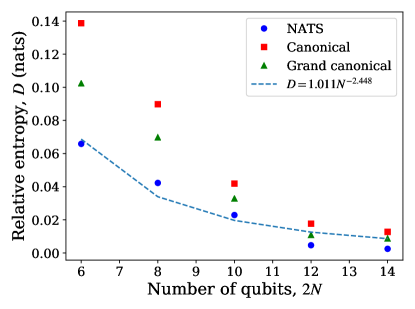
Figure 2: Distances from the long-time state to thermal states: A chain of qubits subject to periodic boundary conditions was simulated numerically. The first preparation protocol and the evolution in Sec. I thermalized a two-qubit system ${\rm S}$ of interest to a long-time state $\rho_{\rm S}$. Plotted is the relative-entropy distance [Eq. (13)] from $\rho_{\rm S}$ to each of three thermal states: the NATS [Eq. (2)] (blue dots), the canonical state (red squares), and a grand canonical state $\propto e^{-\beta(H^{\rm S}-\mu_{z}\sigma_{z}^{\rm S})}$ (green triangles). The NATS theory predicts $\rho_{\rm S}$ with greater accuracy, which grows with the spin-chain size, for finite systems. The dashed line represents the best polynomial fit. Entropies are expressed in units of nats (not to be confused with the NATS: logarithms are base-$e$).

The final system-of-interest state $\rho_{\rm S}$ was compared to the NATS prediction (2), to the canonical prediction (1), and to a grand canonical state $\rho_{\rm GC}\propto e^{-\beta(H^{\rm S}-\mu_{z}\sigma_{z}^{\rm S})}$ that follows from ignoring the conservation of two noncommuting charges. The canonical and grand canonical comparisons were modeled on the comparison to microcanonical and grand canonical predictions in the original GGE studies Rigol_07_Relaxation ; Rigol_09_Breakdown . The canonical state’s $\beta$ equals the NATS’s to first order in the dimensionless parameters [Eq. (10)]. The more-precise versions of inequalities (10) (App. F) were satisfied: Each small parameter was an order of magnitude less than 1.

Figure 2 shows the relative entropies. The blue dots show $D(\rho_{\rm S}||\rho_{\rm NATS})$; the red squares, $D(\rho_{\rm S}||\rho_{\rm can})$; and the green triangles, $D(\rho_{\rm S}||\rho_{\rm GC})$. The NATS theory predicts $\rho_{\rm S}$ with greater accuracy, which grows with the spin chain.

The dashed line shows the best polynomial fit, which scales as approximately $N^{-5/2}$. This fit merits comparison with the right-hand side of Eq. (14). As the system size $N$ grows, the best fit shrinks more quickly than the $\sim N^{-1/2}$ prediction in NYH_16_Microcanonical . This contrast suggests two possibilities: (i) A bound tighter than that in NYH_16_Microcanonical can be proved. (ii) “Transients,” such as $\sim N^{-5/2}$, dominate the scaling at small system sizes. The transients vanish quickly as $N$ grows, and $\sim N^{-1/2}$ dominates the scaling at large system sizes.

As the whole system grows, the NATS, grand canonical, and canonical predictions appear to converge. On the right-hand side of Fig. 2, the blue circle, green triangle, and red square clump close together. This converge is believed to result from the largeness of $T$ and the smallness of the $\mu_{\alpha}$’s. When the temperature is high, all thermal ensembles resemble the maximally mixed state, $\mathbbm{1}/2^{Nn}$. The predictions are expected to separate as $T$ falls and the $\mu_{\alpha}$’s grow.

In experiments, a Hamiltonian close to have the Heisenberg form $\sum_{\alpha}\sigma_{\alpha}^{(j)}\sigma_{\alpha}^{(j+1)}$ can suffer from anisotropies Fukuhara_13_Microscopic . Appendix H demonstrates our protocol’s robustness with respect to realistic anisotropies.

III Discussion

We have formulated and simulated an experimental protocol for thermalizing a quantum many-body system to the NATS. The protocol holds promise for ultracold atoms, trapped ions, quantum dots, nitrogen-vacancy centers, and NMR. This work initiates a bridge from the abstract, idealized NATS theory of QI-theoretic thermodynamics to many-body physics: We introduce noncommutation—a key feature of nonclassicality—of charges into condensed matter and AMO physics. Extensions to high-energy physics beg to be realized. Below, we contrast the NATS with the GGE. Similarly, in App. A, we detail how noncommuting charges invalidate predictions by the ETH. However, Deutsch’s original argument for studying the ETH provides extra motivation for studying the NATS (App. I). Then, we present opportunities for future research.

The GGE is an ensemble to which quantum systems equilibrate if extensively many nontrivial charges are conserved Rigol_09_Breakdown ; Rigol_07_Relaxation ; Vidmar_16_Generalized . Our prediction lies outside existing GGE studies for three reasons. First, GGE studies have not emphasized noncommutation (though noncommuting charges have now appeared in Fagotti_14_On ). Second, the GGE was designed for integrable Hamiltonians. Our Hamiltonian is nonintegrable, because we study thermalization. Third, the charges conserved in GGE problems tend not to equal sums of local charges. Our globally conserved charges do, in the spirit of the textbook problem reviewed in the introduction. We maintain this spirit to emphasize that beginning with a textbook problem and introducing the minimal noncommutative tweak unmoors conventional expectations, as explained in the paragraph above Eq. (2). Our work moors this nonclassical thermalization to an experimental protocol and numerical simulations.

This paper opens up several opportunities for future research. In condensed-matter, AMO, and high-energy physics have recently emerged toolkits for studying many-body thermalization: quantum-simulator experiments Neill_16_Ergodic ; Smith_16_Many ; Bernien_17_Probing ; Wei_18_Emergent ; Kucsko_18_Critical , the ETH Deutsch_91_Quantum ; Srednicki_94_Chaos ; Rigol_08_Thermalization , random unitary circuits Brown_12_Scrambling ; Nahum_18_Operator ; Khemani_18_Operator ; HunterJones_18_Operator , the GGE Rigol_07_Relaxation ; Rigol_09_Breakdown ; Langen_15_Experimental , and out-of-time-ordered correlators Swingle_18_Quantitative . These toolkits should and can be generalized to accommodate noncommuting charges, now that such charges have been imported from QI-theoretic thermodynamics into many-body physics.

Furthermore, these frameworks can be leveraged to explore noncommutation’s effects on thermalization. Constraining dynamics, noncommutation might slow the transport of energy, information, and/or charges. Hence noncommutation might enhance storage and memory. Additionally, noncommutation underlies quantum error correction, quantum cryptography, and other applications. Noncommutation might advance information processing in materials. Furthermore, group theory structures high-energy physics. Non-Abelian groups therein might give rise to NATS physics.

The thermodynamic limit, too, merits study. We focus on experimentally realizable systems, of finite size $N$. Figure 2 suggests that, as the whole system grows, the canonical prediction’s accuracy grows. How much the NATS prediction outperforms the canonical as $N\to\infty$ remains an open question.

Degeneracies suggest more questions: The ETH elucidates how quantum many-body systems thermalize under nondegenerate Hamiltonians. Conserved charges introduce degeneracies, which can affect thermodynamic ensembles. We address degeneracy through the microcanonical lens of NYH_16_Microcanonical : Noncommutation can prevent the charges from sharing an eigenspace. No degenerate microcanonical subspace necessarily exists. The microcanonical subspace was therefore generalized to the a.m.c. subspace NYH_16_Microcanonical . We have proposed protocols for preparing a global system in an a.m.c. subspace. This QI-thermodynamic approach to degeneracy should be complemented with a many-body-physics approach.

Appendix A Protocol’s inequivalence to thermalization under a Hamiltonian that has only U(1) symmetry

One might worry that our protocol’s final state could be predicted without the NATS theory, that the NATS adds nothing to our knowledge of thermalization. Prima facie, the prediction seems to require knowledge of only the ETH and thermalization under U(1)-symmetric Hamiltonians. The latter thermalization has been studied in, e.g., Khemani_18_Operator ; HunterJones_18_Operator . A U(1)-symmetric qubit Hamiltonian conserves $\sigma_{z}^{\rm tot}$. The Hamiltonian is equivalent, via a Jordan-Wigner transformation, to a Hamiltonian that conserves particle number. Hence systems thermalize to the grand canonical ensemble under U(1)-symmetric evolution. This thermalization, we show, is inequivalent to our protocol’s thermalization: Justifiably predicting our protocol’s final state requires knowledge of the NATS. Afterward, we present three more reasons for the inequivalence of thermalization to the NATS and thermalization under a U(1)-symmetric Hamiltonian: First, microscopic dynamics distinguish the two thermalization processes. Second, thermalization to the NATS is inequivalent to thermalization to the grand canonical ensemble just as thermalization to the grand canonical state is inequivalent to thermalization to the canonical state. Third, our thermalization protocol and thermalization to the grand canonical state lead to thermal states whose group-theoretic properties differ.

A brief review of the ETH is in order Deutsch_91_Quantum ; Srednicki_94_Chaos ; Rigol_08_Thermalization ; D'Alessio_16_From . The ETH governs a chaotic quantum many-body system evolving under a nondegenerate Hamiltonian $H^{\rm tot}=\sum_{m}E_{m}\lvert m\rangle\!\langle m\rvert$. Suppose that $H^{\rm tot}$ conserves no nontrivial charges. Let $O$ denote a local observable. A matrix with elements $O_{mn}$ represents $O$ relative to the energy eigenbasis. The diagonal elements $O_{mm}$ vary little with $m$, according to the ETH. Furthermore, off-diagonal elements $O_{m(n\neq m)}$ are exponentially small in the system size. The ETH implies ergodicity, thermalization to a microcanonical (or canonical) expectation value Rigol_12_Alternatives . In many studies, $H^{\rm tot}$ conserves a charge, such as $\sigma_{z}^{\rm tot}$. The ETH is justified within a charge sector.

First, we elucidate why our protocol’s final state appears predictable with just knowledge of the NATS and of thermalization under U(1)-symmetric Hamiltonians. Imagine learning our protocol’s initial state, $\rho$, and Hamiltonian, $H^{\rm tot}$. Imagine having to predict the final state’s form without knowing the NATS theory. One might reason as follows: $H^{\rm tot}$ has SU(2) symmetry. $\sigma_{x}^{\rm tot}$, $\sigma_{y}^{\rm tot}$ and $\sigma_{z}^{\rm tot}$ generate SU(2). Hence the evolution conserves $\left\langle\sigma_{\alpha}^{\rm tot}\right\rangle={\rm Tr}\left(\rho\sigma_{\alpha}^{\rm tot}\right)$ for all $\alpha=x,y,z$. The expectation values form a vector $(\left\langle\sigma_{x}^{\rm tot}\right\rangle,\left\langle\sigma_{y}^{\rm tot}\right\rangle,\left\langle\sigma_{z}^{\rm tot}\right\rangle)\equiv r\hat{r}$. The coordinate system can be transformed such that $\hat{r}$ coincides with the new $z$-direction, $\hat{z^{\prime}}$. The transformation conserves $H^{\rm tot}$. In this reference frame, only $\left\langle\sigma_{z^{\prime}}^{\rm tot}\right\rangle\neq 0$. Furthermore, $\left\langle\sigma_{z^{\prime}}^{\rm tot}(t)\right\rangle$ remains constant. The thermalization therefore appears, prima facie, identical to thermalization under a U(1)-symmetric Hamiltonian. One might therefore predict that the system of interest thermalizes to a grand canonical state in this reference frame. Knowing the ETH, one might predict Eq. (3), wherein $\sum_{\alpha}\mu_{\alpha}Q_{\alpha}=\mu_{z^{\prime}}\sigma_{z^{\prime}}^{\rm tot}$, despite misrepresenting the microscopic dynamics (see below). One could extrapolate the ETH to reconstruct the NATS prediction. Without the NATS theory, however, this prediction would have even less justification than most ETH claims. (The ETH remains a hypothesis. Analytical support for the ETH remains under construction.)

The ETH implies thermalization when the initial state’s support lies on a small microcanonical window of energy levels. Consider the extension of the ETH to the grand canonical ensemble. The Hamiltonian shares an eigenbasis with the particle-number operator. The extension is justified when the initial state’s weight lies on a small microcanonical window of shared eigenstates. Now, consider extending the ETH to thermalization under a Hamiltonian that conserves noncommuting charges $Q_{\alpha}^{\rm tot}$. One would naïvely expect the extension to be justified when the initial state’s support lies on a small microcanonical window of eigenstates shared by $H^{\rm tot}$ and all the $Q_{\alpha}^{\rm tot}$’s. Earlier studies of thermalization in the presence of U(1) symmetry would support the extension. But the $Q_{\alpha}^{\rm tot}$’s do not necessarily share eigenstates, as they fail to commute. Hence an extension of the ETH seems impossible to justify…unless the notion of a microcanonical subspace is generalized to an approximate microcanonical subspace. This generalization forms a cornerstone of the NATS theory NYH_16_Microcanonical . Hence the NATS theory is necessary for justifiably predicting the state to which our system thermalizes. This paper shows that the prediction is accurate for finite-size spin chains evolving under Eq. (8).

NATS thermalization is inequivalent to thermalization under a U(1)-symmetric Hamiltonian for three more reasons. First, under U(1) symmetry, just two quantities hop between subsystems: energy and quanta of one component of angular momentum. Quanta of all three components of the angular momentum—charges that fail to commute with each other—hop during thermalization to the NATS. One misrepresents the microscopic dynamics when attempting to reduce NATS thermalization to thermalization under a U(1)-symmetric Hamiltonian.

The attempt’s failure parallels the failure to reduce grand canonical thermalization to canonical thermalization. The grand canonical state is $\propto e^{-\beta(H-\mu N)}$, wherein $H$ denotes a Hamiltonian, $N$ denotes a particle-number operator, and $\mu$ denotes a chemical potential. One can define an effective Hamiltonian $\tilde{H}:=H-\mu N$. The grand canonical state will look identical to a canonical state, $\propto e^{-\beta\tilde{H}}$. But this definition cannot reduce grand canonical physics to canonical physics. During thermalization to the canonical state, subsystems exchange only energy. During thermalization to the grand canonical state, subsystems exchange energy and particles. The very existence of the name “grand canonical” implies that the energy-and-particle problem differs significantly from the canonical problem and deserves independent consideration. Analogously, one can redefine the $z$-axis such that the NATS state in (3) looks identical to the grand canonical ensemble. But this redefinition cannot reduce NATS thermalization to grand canonical, just as a definition cannot reduce grand canonical to canonical.

Finally, if the Hamiltonian has only U(1) symmetry, the thermal state is proportional to an exponential that contains a Hamiltonian that has only U(1) symmetry. The NATS contains a Hamiltonian that has a non-Abelian symmetry. The two states have different group-theoretic properties.

Appendix B In every short-range-correlated state, each total spin component has a subextensive standard deviation.

Consider an arbitrary short-range-correlated state of correlation length $\xi$. Let $\left\langle O\right\rangle$ denote the expectation value of an observable $O$ in that state. By assumption,

$$\left\langle\sigma_{\alpha}^{(j)}\sigma_{\alpha}^{(j^{\prime})}\right\rangle-\left\langle\sigma_{\alpha}^{(j)}\right\rangle\left\langle\sigma_{\alpha}^{(j^{\prime})}\right\rangle\sim e^{-|j-j^{\prime}|/\xi}\,.$$ (B1)

We have set the lattice spacing to one. Let us calculate each term in the standard deviation of $\sigma_{\alpha}^{\rm tot}$,

$$\sqrt{\left\langle(\sigma_{\alpha}^{\rm tot})^{2}\right\rangle-\left\langle\sigma_{\alpha}^{\rm tot}\right\rangle^{2}}\,.$$ (B2)

The first term has the form

$$\left\langle(\sigma_{\alpha}^{\rm tot})^{2}\right\rangle =\left\langle\left(\sum_{j=1}^{Nn}\sigma_{\alpha}^{(j)}\right)\left(\sum_{j^{\prime}=1}^{Nn}\sigma_{\alpha}^{(j^{\prime})}\right)\right\rangle=\left\langle\sum_{j=1}^{Nn}(\sigma_{\alpha}^{(j)})^{2}\right\rangle+\sum_{j\neq j^{\prime}}\left\langle\sigma_{\alpha}^{(j)}\sigma_{\alpha}^{(j^{\prime})}\right\rangle.$$ (B3)

The first term on the right-hand side of Eq. (B3) simplifies as

$$\left\langle\sum_{j=1}^{Nn}(\sigma_{\alpha}^{(j)})^{2}\right\rangle =\sum_{j=1}^{Nn}\left\langle\mathbbm{1}_{2}^{\otimes Nn}\right\rangle=Nn.$$ (B4)

The second term on the right-hand side of Eq. (B3) simplifies under assumption (B1):

$$\sum_{j\neq j^{\prime}}\left\langle\sigma_{\alpha}^{(j)}\sigma_{\alpha}^{(j^{\prime})}\right\rangle\sim\sum_{j\neq j^{\prime}}\left\langle\sigma_{\alpha}^{(j)}\right\rangle\left\langle\sigma_{\alpha}^{(j^{\prime})}\right\rangle+\sum_{j\neq j^{\prime}}e^{-|j-j^{\prime}|/\xi}.$$ (B5)

The second term has significant contributions only from subterms in which $j^{\prime}$ lies within $\xi$ of $j$. Hence the $e^{-|j-j^{\prime}|/\xi}\sim e^{-\xi/\xi}={\rm const.}$ A constant number of such subterms exist. Hence the right-hand side of Eq. (B5) can be approximated with

$$\sum_{j\neq j^{\prime}}\left\langle\sigma_{\alpha}^{(j)}\sigma_{\alpha}^{(j^{\prime})}\right\rangle\sim\sum_{j\neq k}\left\langle\sigma_{\alpha}^{(j)}\right\rangle\left\langle\sigma_{\alpha}^{(j^{\prime})}\right\rangle+Nn.$$ (B6)

Substituting from Eqs. (B4) and (B6) into the right-hand side of Eq. (B3) yields

$$\left\langle(\sigma_{\alpha}^{\rm tot})^{2}\right\rangle \sim Nn+\sum_{j\neq j^{\prime}}\left\langle\sigma_{\alpha}^{(j)}\right\rangle\left\langle\sigma_{\alpha}^{(j^{\prime})}\right\rangle.$$ (B7)

Let us estimate the second term in (B2):

$$\left\langle\sigma_{\alpha}^{\rm tot}\right\rangle^{2} =\left\langle\sum_{j=1}^{Nn}\sigma_{\alpha}^{(j)}\right\rangle^{2}=\left(\sum_{j=1}^{Nn}\left\langle\sigma_{\alpha}^{(j)}\right\rangle\right)^{2}=\left(\sum_{j=1}^{Nn}\left\langle\sigma_{\alpha}^{(j)}\right\rangle\right)\left(\sum_{j^{\prime}=1}^{Nn}\left\langle\sigma_{\alpha}^{(j^{\prime})}\right\rangle\right)$$ (B8)

$$=\sum_{j=1}^{Nn}\left\langle\sigma_{\alpha}^{(j)}\right\rangle^{2}+\sum_{j\neq j^{\prime}}\left\langle\sigma_{\alpha}^{(j)}\right\rangle\left\langle\sigma_{\alpha}^{(j^{\prime})}\right\rangle$$ (B9)

$$\sim Nn+\sum_{j\neq j^{\prime}}\left\langle\sigma_{\alpha}^{(j)}\right\rangle\left\langle\sigma_{\alpha}^{(j^{\prime})}\right\rangle.$$ (B10)

We have approximated the first term with $(\text{number of terms})(\text{operator norm of }\sigma_{\alpha}^{(j)})$. Let us substitute from Eqs. (B7) and (B10) into Eq. (B2). The $\sum_{j\neq k}$ terms cancel exactly, leaving

$$\sqrt{\left\langle(\sigma_{\alpha}^{\rm tot})^{2}\right\rangle-\left\langle\sigma_{\alpha}^{\rm tot}\right\rangle^{2}}\sim\sqrt{Nn}.$$ (B11)

Appendix C Soft measurement

This appendix details the soft measurements introduced in Sec. I. We formalize soft measurements in App. C 1. Appendix C 2 provides physical intuition about the preparation procedure that relies on soft measurements.

C 1 Formalization of soft measurements

We formalize soft measurements with a positive operator-valued measure (POVM). POVMs model generalized measurements in QI theory NielsenC10 . A POVM consists of positive operators $M_{\ell}>0$, called Kraus operators. They satisfy the completeness relation $\sum_{\ell}M_{\ell}^{\dagger}M_{\ell}=\mathbbm{1}$. Measuring the $\left\{M_{\ell}\right\}$ of a state $\rho$ has a probability ${\rm Tr}(M_{\ell}^{\dagger}M_{\ell}\rho)$ of yielding outcome $\ell$. The measurement updates $\rho$ to $M_{\ell}\rho M_{\ell}^{\dagger}/{\rm Tr}(M_{\ell}^{\dagger}M_{\ell}\rho)$. Let $P_{\alpha}^{S_{\alpha}}$ denote the projector onto the eigenvalue-$S_{\alpha}$ eigenspace of $\sigma_{\alpha}^{\rm tot}$. A soft $\sigma_{\alpha}^{\rm tot}$ measurement has the form $\{M_{\alpha}^{S_{\alpha}}\}$. The outcome $S_{\alpha}$ labels the Kraus operators,

$$M_{\alpha}^{S_{\alpha}}=\sum_{\tilde{S}_{\alpha}=-Nn,-Nn+2,\ldots,Nn-2,Nn}\sqrt{f_{Nn}(S_{\alpha},\tilde{S}_{\alpha})}\;P_{\alpha}^{\tilde{S}_{\alpha}}.$$ (C1)

Outputting $S_{\alpha}$, the measurement projects the state a little onto each of the eigenspaces in superposition. How much does the measurement project onto the eigenspace associated with some eigenvalue $\tilde{S}_{\alpha}$? The amount depends on the amplitude $f_{Nn}(S_{\alpha},\tilde{S}_{\alpha})$. The amplitude must maximize where $S_{\alpha}=\tilde{S}_{\alpha}$, to satisfy the peaking requirement (Sec. I). The binomial distribution suggests itself. We present the distribution, then derive and analyze it:

$$f_{Nn}(S_{\alpha},\tilde{S}_{\alpha}) ={Nn\choose\frac{1}{2}(Nn+S_{\alpha})}\left[\frac{1}{2}\left(1+\frac{\tilde{S}_{\alpha}}{Nn}\right)\right]^{\frac{1}{2}(Nn+S_{\alpha})}\left[\frac{1}{2}\left(1-\frac{\tilde{S}_{\alpha}}{Nn}\right)\right]^{\frac{1}{2}(Nn-S_{\alpha})}\,.$$ (C2)

We define $0^{0}\equiv 1$. Numerics confirm that the POVM (C1) satisfies the mild-disturbance condition (ii) in Sec. I.

The envelope (C2) is constructed as follows. We semiclassically model each qubit as pointing upward or downward along the $\alpha$-axis. We formulate the binomial probability that an $(Nn)$-qubit chain has a magnetization $S_{\alpha}$, if the average-over-trials magnetization equals $\tilde{S}_{\alpha}$. Let $n_{\uparrow}$ and $n_{\downarrow}$ denote the numbers of upward- and downward-pointing qubits in some configuration. Let $p_{\uparrow}$ denote the probability that a given qubit points upward and $p_{\downarrow}$, the probability that the qubit points downward. We must solve for each of these quantities in terms of $S_{\alpha}$, $\tilde{S}_{\alpha}$, and $Nn$. As $Nn=n_{\uparrow}+n_{\downarrow}$ and $S_{\alpha}=n_{\uparrow}-n_{\downarrow}$, $n_{\uparrow}=\frac{1}{2}(Nn+S_{\alpha})$, and $n_{\downarrow}=\frac{1}{2}(Nn-S_{\alpha})$. On average, $\tilde{S}_{\alpha}=(p_{\uparrow}-p_{\downarrow})Nn$ qubits point upward. By normalization, $p_{\downarrow}=1-p_{\uparrow}$. Hence $p_{\uparrow}=\frac{1}{2}\left(1+\frac{\tilde{S}_{\alpha}}{Nn}\right)$, and $p_{\downarrow}=\frac{1}{2}\left(1-\frac{\tilde{S}_{\alpha}}{Nn}\right)$. The binomial function has the form $f_{Nn}(S_{\alpha},\tilde{S}_{\alpha})={Nn\choose n_{\uparrow}}(p_{\uparrow})^{n_{\uparrow}}(p_{\downarrow})^{n_{\downarrow}}.$ Substituting in yields Eq. (C2).

As $Nn\to\infty$, the binomial approaches a Gaussian. The Gaussian has a mean of $\left\langle S_{\alpha}\right\rangle=\tilde{S}_{\alpha}$ and a standard deviation of

$$\Delta=\frac{1}{2}\sqrt{Nn\left(1+\frac{\tilde{S}_{\alpha}}{Nn}\right)\left(1-\frac{\tilde{S}_{\alpha}}{Nn}\right)}\sim\sqrt{Nn}.$$ (C3)

Hence

$$\lim_{Nn\to\infty}f_{Nn}(S_{\alpha},\tilde{S}_{\alpha})=\exp\left(-\frac{(S_{\alpha}-\tilde{S}_{\alpha})^{2}}{2\Delta^{2}}\right)\Big{/}\sqrt{2\pi\Delta^{2}}\,.$$ (C4)

Prima facie, $S_{\alpha}$ and $\tilde{S}_{\alpha}$ appear to have been swapped relative to their natural roles: $S_{\alpha}$ was defined as the “expected” $\sigma_{\alpha}^{\rm tot}$ value in Sec. I. But $\tilde{S}_{\alpha}$ determines the mean spin in Eq. (C2). This swap impacts the function’s behavior little: $f_{Nn}(S_{\alpha},\tilde{S}_{\alpha})$ peaks at $S_{\alpha}=\tilde{S}_{\alpha}$. The peak grows higher and narrower as $Nn$ grows. As $Nn\to\infty$, the envelope approaches a Gaussian symmetric under $S_{\alpha}\leftrightarrow\tilde{S}_{\alpha}$ [Eq. (C4)]. Normalization motivates the swap: The POVM (C1) must satisfy the completeness condition $\sum_{S_{\alpha}}(M_{\alpha}^{S_{\alpha}})^{\dagger}M_{\alpha}^{S_{\alpha}}=\mathbbm{1}$. The POVM does because the envelope is normalized as $\sum_{S_{\alpha}}f_{Nn}(S_{\alpha},\tilde{S}_{\alpha})=1$.

C 2 Physical intuition about the soft-measurement preparation procedure

Suppose that the spin chain begins in a random state. Measuring $H^{\rm tot}$ with decent precision projects the chain’s state approximately onto an energy eigenspace. This eigenspace is larger than the a.m.c. subspace, $\mathcal{M}$. The soft $x$ measurement collapses the state a little, shrinking the state’s support. The soft $y$ and $z$ measurements shrink the support further. After the final measurement, at least most of the state’s support lies in $\mathcal{M}$, as quantified in App. E. Figure 3 sketches the relationships amongst the subspaces.

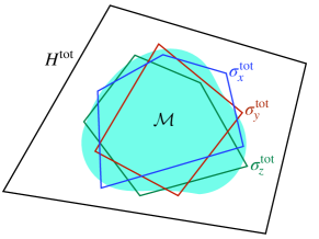
Figure 3: Sketch of subspaces: The black, outermost line represents an eigenspace of the total Hamiltonian, $H^{\rm tot}$. Inside lies the approximate microcanonical subspace, $\mathcal{M}$, represented by the shaded shape. $\mathcal{M}$ generalizes the microcanonical subspace to noncommuting exchanged charges. The total-spin components $\sigma_{\alpha=x,y,z}^{\rm tot}$ have eigenspaces that largely coincide with $\mathcal{M}$.

Let us illustrate how each soft measurement partially collapses the spin chain’s state. Consider a toy system of $Nn=2$ qubits whose $\sigma_{z}^{\rm tot}$ and $\sigma_{x}^{\rm tot}$ are measured softly. Suppose that the measurements yield $S_{z},S_{x}=0$. The conditioned soft $z$ measurement projects the state with $P_{z}^{0}\propto M_{z}^{0}$, by Eqs. (C1) and (C2). $P_{z}^{0}$ projects onto the eigenvalue-0 eigenspace of $\sigma_{z}^{\rm tot}$. This eigenspace is spanned by the singlet $\lvert s_{z}\rangle:=\frac{1}{\sqrt{2}}\>(\lvert z+,z-\rangle-\lvert z-,z+\rangle)$ and the entangled triplet $\lvert t_{z}\rangle:=\frac{1}{\sqrt{2}}\>(\lvert z+,z-\rangle+\lvert z-,z+\rangle)$. That is, $P_{z}^{0}=\lvert s_{z}\rangle\!\langle s_{z}\rvert+\lvert t_{z}\rangle\!\langle t_{z}\rvert$. Similarly, the conditioned $x$ measurement projects the state with $P_{x}^{0}=\lvert s_{x}\rangle\!\langle s_{x}\rvert+\lvert t_{x}\rangle\!\langle t_{x}\rvert$.

Onto what subspace does the sequence of approximate measurements project? Let us express $P_{x}^{0}$ in terms of the $z$-type singlet and triplets. The singlet relative to any axis equals the singlet relative to every other, to within a global phase: $\lvert s_{x}\rangle=(\text{phase})\lvert s_{z}\rangle$. The $x$-type entangled triplet decomposes as $\lvert t_{x}\rangle\propto\frac{1}{\sqrt{2}}\>(\lvert z+,z+\rangle-\lvert z-,z-\rangle)$. Hence $P_{x}^{0}P_{z}^{0}=\lvert s_{z}\rangle\!\langle s_{z}\rvert$. The approximate $\sigma_{z}^{\rm tot}$ measurement collapses the state onto a two-dimensional subspace; and the approximate $\sigma_{x}^{\rm tot}$ measurement, onto a one-dimensional subspace.

Appendix D Standard deviations in global charges $\sigma_{\alpha}^{\rm tot}$ after a sequence of soft measurements

Section I B and App. C introduce the soft-measurement protocol for preparing a global state $\rho^{\rm tot}$ in an a.m.c. subspace. $\rho^{\rm tot}$ should exhibit property (i): In $\rho^{\rm tot}$, every global charge $\sigma_{\alpha}^{\rm tot}$ should have a standard deviation that grows with the system size, $Nn$, no more than linearly. The need for slow scaling motivated soft measurements’ “mild-disturbance” property. Here, we numerically check the standard-deviation scaling at infinite temperature.

Setting $T=\infty$ obscures the distinction between the NATS and other thermodynamic ensembles as measured in Sec. II. However, this study offers two benefits: First, these initial results motivate detailed numerics, at large system sizes, outside the scope of this paper. Second, $T=\infty$ will not necessarily hinder future thermodynamic studies of noncommuting charges.

We checked the standard deviations with the following protocol:

1. Prepare the global system in a random pure initial state Zyczkowski_11_Generating : Form a superposition of all the $\sigma_{z}$ product states. Choose each amplitude’s real part according to the standard normal distribution. Choose the amplitude’s imaginary part, independently, according to the same distribution. Normalize the state.

2. Measure $\sigma_{x}^{\rm tot}$ softly.

3. Measure $\sigma_{y}^{\rm tot}$ softly.

4. Measure $\sigma_{z}^{\rm tot}$ softly.

5. Compute the standard deviation $\sqrt{\left\langle(\sigma_{\alpha}^{\rm tot})^{2}\right\rangle-\left\langle\sigma_{\alpha}^{\rm tot}\right\rangle^{2}}$ for every $\alpha$.

6. Perform steps 1–5 for each of 100 random initial states.

7. For each $\alpha$, average the standard deviation $\sqrt{\left\langle(\sigma_{\alpha}^{\rm tot})^{2}\right\rangle-\left\langle\sigma_{\alpha}^{\rm tot}\right\rangle^{2}}$ over the states.

Figure 4 shows the state-averaged standard deviations plotted against the global system size, $Nn$. The curves show the best fits of the form $({\rm const.})(Nn)^{{\rm const.}}$. If $\alpha=x,y$, the exponents are $0.277,0.381<0.5$, as required in property (i) of Sec. I B.

If $\alpha=z$, the exponent lies slightly above $0.5$, at $0.566$. The reason is, $\sigma_{z}^{\rm tot}$ was softly measured last: In another study we softly measured $\sigma_{z}^{\rm tot}$, then $\sigma_{x}^{\rm tot}$, then $\sigma_{y}^{\rm tot}$. The last-measured charge scales with the greatest exponent, $0.612$. However, the second-measured charge, $\sigma_{x}^{\rm tot}$, scales with the least exponent. In contrast, in Fig. 4, the first-measured charge, $\sigma_{x}^{\rm tot}$ scales with the least exponent. We expect this discrepancy, as well as the slightly-above-$0.5$ exponent, to disappear as the global system grows: Large numbers promote internal averaging.

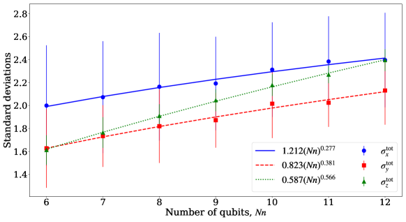
Figure 4: Standard deviations in global charges $\sigma_{\alpha}^{\rm tot}$ after a sequence of soft measurements: Each standard deviation has been averaged over 100 random initial global states, which mimic infinite-temperature states. The curves depict the best fits of the form $({\rm const.})(Nn)^{{\rm const.}}$.

Appendix E Parameterization of the approximate microcanonical subspace

An a.m.c. subspace $\mathcal{M}$ is defined in terms of five small parameters NYH_16_Microcanonical . They govern the constants in Ineq. (14), the bound on the distance between $\rho_{\rm S}$ and the NATS. The constants’ forms are calculated partially in NYH_16_Microcanonical . Calculating them completely would require experiments or extensive analytics. We review the a.m.c. subspace’s definition in Sec. E 1. In Sec. E 2, we identify parameter values suited to our protocol. We focus on the soft-measurement state preparation for concreteness.

E 1 Definition of the a.m.c. subspace

$\mathcal{M}$ is defined in terms of two conditions NYH_16_Microcanonical : (i) Every state in $\mathcal{M}$ has a fairly well-defined value of each $\sigma_{\alpha}^{\rm tot}$. (ii) Consider state whose $\sigma_{\alpha}^{\rm tot}$ has a fairly well-defined value for every $\alpha$. Most of the state’s support lies in $\mathcal{M}$. These conditions are quantified in terms of small parameters $\delta,\eta,\delta^{\prime},\eta^{\prime},\epsilon\gtrsim 0$.

(i) Let $\omega$ denote any whole-system state supported in just $\mathcal{M}$. In $\omega$, every total charge has a fairly well-defined value: Consider measuring any $\sigma_{\alpha}^{\rm tot}$. The measurement has a high probability of yielding an outcome close to the “expected value” $S_{\alpha}$. (The notation $v_{\alpha}=\frac{S_{\alpha}}{N}$ is used in NYH_16_Microcanonical .) Consider a narrow strip of $\sigma_{\alpha}^{\rm tot}$ eigenvalues centered on $S_{\alpha}$. Recall that the system-of-interest charge $\sigma_{\alpha}^{(j)}+\sigma_{\alpha}^{(j+1)}$ has a spectral diameter of two. The strip is therefore chosen to extend a distance $2\eta N$ on either side of $S_{\alpha}$. Consider the $\sigma_{\alpha}^{\rm tot}$ eigenvalues in $[S_{\alpha}-2\eta N,\>S_{\alpha}+2\eta N]$. They correspond to eigenspaces whose direct sum is projected onto by $\Pi^{\eta}_{\alpha}$. A $\sigma_{\alpha}^{\rm tot}$ measurement has a probability ${\rm Tr}(\omega\Pi^{\eta}_{\alpha})$ of yielding a value in this interval. The probability must be at least $1-\delta$:

$$\operatorname{supp}(\omega)\subset\mathcal{M}\qquad\Rightarrow\qquad{\rm Tr}(\omega\Pi^{\eta}_{\alpha})\geq 1-\delta\quad\forall\alpha.$$ (E1)

(ii) Let $\omega^{\prime}$ denote any state for which measuring any $\sigma_{\alpha}^{\rm tot}$ has a high probability of yielding an outcome close to the expected value, within $2\eta^{\prime}Nn$ of $S_{\alpha}$. Most of the support of $\omega^{\prime}$ lies in $\mathcal{M}$—at least a fraction $1-\epsilon$. As $P_{\mathcal{M}}$ denotes the projector onto the a.m.c. subspace,

$${\rm Tr}\left(\omega^{\prime}\Pi^{\eta^{\prime}}_{\alpha}\right)\geq 1-\delta^{\prime}\quad\forall\alpha\qquad\Rightarrow\qquad{\rm Tr}(\omega^{\prime}P_{\mathcal{M}})\geq 1-\epsilon.$$ (E2)

E 2 Parameter values suited to the soft-measurement preparation procedure

We have freedom in choosing the parameters’ values: We have specified a procedure for preparing a global state $\rho_{\rm tot}$ that has substantial support on an a.m.c. subspace $\mathcal{M}$. In fact, $\rho_{\rm tot}$ might have much support on each of multiple a.m.c. subspaces. Hence we may be able to specify one of multiple possible sets of parameter values.

Three principles guide our choice: informativeness, tradeoffs, and the soft measurement’s form. First, some choices of parameters are less informative than others. The greater the parameters, the less an a.m.c. subspace $\mathcal{M}$ resembles a microcanonical subspace, the less the global system is expected to thermalize internally, and the looser the bound on $D(\rho_{\rm S}||\rho_{\rm NATS})$ is expected to be. Yet the parameters cannot be arbitrarily small, because they trade off, second. For example, the lesser the $\eta$, the greater $\delta$ will tend to be, by the inequality in (E1). Third, the soft measurement’s form points to a natural choice of parameter values. For example, $\approx 68\%$ of a Gaussian’s support lies within a standard deviation of its mean. Hence we will choose $\delta^{\prime}=1-0.68$. This choice is not unique but is suggested by the soft measurement’s form.

After the procedure, measuring any $\sigma_{\alpha}^{\rm tot}$ likely yields a value within a standard deviation $\Delta$ of $S_{\alpha}$. The standard deviation scales as $\Delta\sim\sqrt{Nn}$. Hence the procedure prepares an instance of the $\omega^{\prime}$ in (E2), for $2\eta^{\prime}N=({\rm const.})\sqrt{Nn}$. Rearranging yields the first small parameter,

$$\boxed{\eta^{\prime}=({\rm const.})/\sqrt{N}}\,.$$ (E3)

We have incorporated $\sqrt{n}=\sqrt{2}$ into the constant. The spin chain is large, so $\eta^{\prime}$ is small, as desired.

We choose $\delta^{\prime}$ by calculating the left-hand side of the leftmost inequality in (E2), the probability that measuring a $\sigma_{\alpha}^{\rm tot}$ of $\omega^{\prime}$ yields a value within $\Delta$ of $S_{\alpha}$. We integrate $f_{Nn}(S_{\alpha},\tilde{S}_{\alpha})$ across a region, centered on $\tilde{S}_{\alpha}=S_{\alpha}$, of half-width $\Delta$:

$$1-\delta^{\prime}\leq\int_{S_{\alpha}-\Delta}^{S_{\alpha}+\Delta}d\tilde{S}_{\alpha}\;f_{Nn}(S_{\alpha},\tilde{S}_{\alpha}).$$ (E4)

We approximate $f_{Nn}$ with the Gaussian (C4). A Gaussian is well-known to have $68\%$ of its weight within a standard deviation of its mean. Hence we choose $1-\delta^{\prime}=0.68$, or

$$\boxed{\delta^{\prime}=0.32}\,.$$ (E5)

$\delta^{\prime}\ll 1$, as desired.

We have chosen values for two of the five parameters that define an a.m.c. subspace $\mathcal{M}$, $\eta^{\prime}$ and $\delta^{\prime}$. Let us turn to $\eta$, $\delta$, and $\epsilon$. In NYH_16_Microcanonical , $c$ denotes the number of non-Hamiltonian charges. Theorem 4 in (NYH_16_Microcanonical, , Suppl. Inf.) presents a condition under which $\mathcal{M}$ is known to exist. The condition governs the small parameters and the number $N$ of subsystems: For every $\epsilon>(c+1)\delta^{\prime}>0$, $\eta>\eta^{\prime}>0$, $\delta>0$, and all great-enough $N$, “there exists an $\left(\epsilon,\eta,\eta^{\prime},\delta,\delta^{\prime}\right)$-approximate microcanonical subspace $\mathcal{M}$ […] associated with […] the approximate expectation values” $S_{\alpha}$. An $\mathcal{M}$ might exist under other conditions. But these known conditions motivate choices of $\epsilon$ and $\eta$. The theorem suggests choosing

$$\boxed{\eta>\eta^{\prime}=({\rm const.})/\sqrt{N}.}\,.$$ (E6)

By Eq. (E4) and $c=3$,

$$\boxed{\epsilon>(c+1)\delta^{\prime}=1.28}\,,$$ (E7)

Though $\epsilon>1$ contradicts the spirit of the a.m.c. subspace’s definition, the inequality does not contradict the letter.

We have chosen values for all the parameters except $\delta$. The soft-measurement procedure underdetermines $\delta$. For inspiration for our choice of $\delta$, we turn to the a.m.c. subspace’s definition, (E1) and (E2). $\delta$ and $\delta^{\prime}$ play analogous roles. Hence we choose

$$\boxed{\delta=\delta^{\prime}=0.32}\,.$$ (E8)

Appendix F Calculation of the inverse temperature $\beta$ and the effective chemical potentials $\mu_{\alpha}$

Let us derive Eqs. (11) and (12). We index such that ${\rm S}$ consists of qubits $j=1,2,\ldots,n$. This choice is for convenience, and ${\rm S}$ lies far from the boundaries. We assume that the temperature is high and the chemical potentials are low: Calculations are to first order in the small parameters approximated in the left-hand side of Ineq. (10) and presented precisely below [in Ineq. (F14) for closed boundary conditions and in Ineq. (F16) for periodic]. We calculate the partition function, then $\beta$, and then the $\mu_{\alpha}$’s. Rewriting Eq. (8) will prove convenient:

$$H^{\rm tot}=J\sum_{\alpha=x,y,z}\left(\sum_{j=1}^{Nn-1}\sigma_{\alpha}^{(j)}\sigma_{\alpha}^{(j+1)}+\sum_{j=1}^{Nn-2}\sigma_{\alpha}^{(j)}\sigma_{\alpha}^{(j+2)}\right).$$ (F1)

This Hamiltonian encodes closed boundary conditions. The numerical simulations (Sec. II) involve periodic boundary conditions. We extend calculations to periodic boundary conditions at the end of the appendix.

Partition function: Let us Taylor-approximate the exponential in the NATS:

$$e^{-\beta\left(H^{\rm tot}-\sum_{\alpha}\mu_{\alpha}\sigma_{\alpha}^{\rm tot}\right)}=\mathbbm{1}-\beta H^{\rm tot}+\beta\sum_{\alpha}\mu_{\alpha}\sigma_{\alpha}^{\rm tot}+O_{2}.$$ (F2)

The exponential’s trace equals $Z$. The linear terms vanish, as ${\rm Tr}(\sigma_{\alpha}^{(j)})=0$ for all $\alpha$ and $j$. Hence

$$Z=2^{Nn}+O_{2}.$$ (F3)

Inverse temperature: $\beta$ follows from the prediction

$$E^{\rm tot}={\rm Tr}\left(H^{\rm tot}e^{-\beta\left(H^{\rm tot}-\sum_{\alpha}\mu_{\alpha}\sigma_{\alpha}^{\rm tot}\right)}\right)/Z.$$ (F4)

We substitute in for the exponential from Eq. (F2), then invoke the trace’s linearity. Terms one and three vanish by the Paulis’ tracelessness:

$$E^{\rm tot}=-\beta{\rm Tr}\left(\left[H^{\rm tot}\right]^{2}\right)/Z+O_{2}.$$ (F5)

Let us evaluate the trace:

$${\rm Tr}\left(\left[H^{\rm tot}\right]^{2}\right) =J^{2}\sum_{\alpha,\alpha^{\prime}}{\rm Tr}\Bigg{(}\sum_{j,j^{\prime}=1}^{Nn-1}\sigma_{\alpha}^{(j)}\sigma_{\alpha}^{(j+1)}\sigma_{\alpha^{\prime}}^{(j^{\prime})}\sigma_{\alpha^{\prime}}^{(j^{\prime}+1)}+\sum_{j=1}^{Nn-1}\sum_{j^{\prime}=1}^{Nn-2}\sigma_{\alpha}^{(j)}\sigma_{\alpha}^{(j+1)}\sigma_{\alpha^{\prime}}^{(j^{\prime})}\sigma_{\alpha^{\prime}}^{(j^{\prime}+2)}$$

$$\qquad\qquad\qquad\;+\sum_{j=1}^{Nn-2}\sum_{j^{\prime}=1}^{Nn-1}\sigma_{\alpha}^{(j)}\sigma_{\alpha}^{(j+2)}\sigma_{\alpha^{\prime}}^{(j^{\prime})}\sigma_{\alpha^{\prime}}^{(j^{\prime}+1)}+\sum_{j=1}^{Nn-2}\sum_{j^{\prime}=1}^{Nn-2}\sigma_{\alpha}^{(j)}\sigma_{\alpha}^{(j+2)}\sigma_{\alpha^{\prime}}^{(j^{\prime})}\sigma_{\alpha^{\prime}}^{(j^{\prime}+2)}\Bigg{)}.$$ (F6)

Most of the terms vanish, by the Paulis’ tracelessness. In each surviving term, $\alpha=\alpha^{\prime}$, $j=j^{\prime}$, and the second Pauli operator acts on the same qubit as the fourth. Every Pauli squares to the identity, $\left(\sigma_{\alpha}^{(j)}\right)^{2}=\mathbbm{1}_{2}$, so

$${\rm Tr}\left(\left[H^{\rm tot}\right]^{2}\right) =J^{2}\sum_{\alpha}\left(\sum_{j=1}^{Nn-1}+\sum_{j=1}^{Nn-2}\right)2^{Nn}$$ (F7)

$$=3(2Nn-3)2^{Nn}J^{2}.$$ (F8)

We substitute into Eq. (F5):

$$E^{\rm tot}=-3(2Nn-3)\beta J^{2}+O_{2}.$$ (F9)

Solving for $\beta$ yields Eq. (11).

Effective chemical potentials: $\mu_{\alpha}$ follows from the prediction

$$S_{\alpha}={\rm Tr}\left(\sigma_{\alpha}^{\rm tot}\,e^{-\beta\left(H^{\rm tot}-\sum_{\alpha^{\prime}}\mu_{\alpha^{\prime}}\sigma_{\alpha^{\prime}}^{\rm tot}\right)}\right)/Z.$$ (F10)

We Taylor-approximate the exponential as in Eq. (F2), then invoke the trace’s linearity. Terms one and two vanish, by the Paulis’ tracelessness:

$$S_{\alpha}=\left[\beta\sum_{\alpha^{\prime}}\mu_{\alpha^{\prime}}{\rm Tr}\left(\sigma_{\alpha}^{\rm tot}\sigma_{\alpha^{\prime}}^{\rm tot}\right)+O_{2}\right]/Z.$$ (F11)

The trace evaluates to

$${\rm Tr}\left(\sigma_{\alpha}^{\rm tot}\sigma_{\alpha^{\prime}}^{\rm tot}\right) =\sum_{j,j^{\prime}=1}^{Nn}{\rm Tr}\left(\sigma_{\alpha}^{(j)}\sigma_{\alpha^{\prime}}^{(j^{\prime})}\right)=Nn\,2^{Nn}\delta_{\alpha\alpha^{\prime}}.$$ (F12)

In the sum’s nonzero terms, the two Pauli operators collide. We substitute into Eq. (F11) and solve for $\mu_{\alpha}$:

$$\mu_{\alpha}=\frac{S_{\alpha}}{Nn\beta}+O_{2}.$$ (F13)

Substituting in for $\beta$ from Eq. (11) yields Eq. (12).

Small-parameter conditions: Inequalities (10) specify loosely when our Taylor approximations hold. More-precise forms for the conditions are presented here. The conditions follow from calculating second-order corrections, then demanding that the corrections be much smaller than the first-order terms:

$$\sqrt{3(2Nn-3)}\>|\beta|J,\;\;\sqrt{Nn\sum_{\alpha}\mu_{\alpha}^{2}}\>|\beta|,\;\;\frac{2}{3}\>\frac{|\beta|\sum_{\alpha}\mu_{\alpha}^{2}}{J},\;\;6\>\frac{Nn-2}{2Nn-3}\>|\beta|J,\;\;4\>\frac{2Nn-3}{Nn}\>|\beta|J\ll 1.$$ (F14)

Periodic boundary conditions: The numerical simulations (Sec. II) involve periodic boundary conditions. The Hamiltonian has the form

$$H^{\rm tot}=J\sum_{\alpha}\sum_{j=1}^{Nn}\left(\sigma_{\alpha}^{(j)}\sigma_{\alpha}^{(j+1)}+\sigma_{\alpha}^{(j)}\sigma_{\alpha}^{(j+2)}\right).$$ (F15)

The site label $j=Nn+1$ is defined as $j=1$, and $j=Nn+2$ is defined as $j=2$. Equation (F8) changes to ${\rm Tr}\left([H^{\rm tot}]^{2}\right)=6Nn2^{Nn}J^{2}$, so $\beta=-\frac{E^{\rm tot}}{6NnJ^{2}}+O_{2}$. The $\mu_{\alpha}$ prediction remains unchanged to first order, though not to second-order. The small-parameter conditions become

$$\sqrt{6Nn}\>|\beta|J,\;\;\frac{2}{3}\>\frac{|\beta|\sum_{\alpha}\mu_{\alpha}^{2}}{J},\;\;8|\beta|J\ll 1.$$ (F16)

Appendix G Quantum state tomography for inferring the long-time system-of-interest state

We aim to observe that ${\rm S}$, the $n$-qubit system of interest, thermalizes to the NATS. The following quantum-state-tomography protocol suffices. A more efficient protocol, that takes advantage of the NATS’s form, might exist.

Let $\vec{\alpha}=(\alpha_{1},\alpha_{2},\ldots,\alpha_{n})$ specify a product $\sigma_{\alpha_{1}}^{(1)}\otimes\sigma_{\alpha_{2}}^{(2)}\otimes\ldots\otimes\sigma_{\alpha_{n}}^{(n)}$ of Pauli operators. $3^{n}$ such products exist. The set of the products’ eigenbases forms a basis for the $n$-qubit Hilbert space. We measure each eigenbasis at the end of each of $\mathcal{N}_{\rm trials}$ trials. Each measurement yields one of $2^{n}$ possible outcomes, $\ell=1,2,\ldots,2^{n}$. If outcome $\ell$ obtains, the projector $\Pi^{\vec{\alpha}}_{\ell}$ projects the state. Each measurement has a probability $p_{\vec{\alpha}}(\ell|\rho_{\rm S})={\rm Tr}(\Pi^{\vec{\alpha}}_{\ell}\rho_{\rm S})$ of yielding outcome $\ell$. Let $f^{\vec{\alpha}}_{\ell}$ denote the frequency with which measuring $\vec{\alpha}$ yields outcome $\ell$ in our $\mathcal{N}_{\rm trials}$ trials. The frequency approximates the probability with an error $\sim 1/\sqrt{\mathcal{N}_{\rm trials}}$.

From the frequencies, we estimate $\rho_{\rm S}$. We can do so by solving the semidefinite program

$$\min_{\rho\,:\,\rho\geq 0,\,{\rm Tr}(\rho)=1}\sum_{\vec{\alpha}\in\{x,y,z\}^{n}}\sum_{\ell=0}^{2^{n}-1}\left[f^{\vec{\alpha}}_{\ell}-{\rm Tr}(\Pi^{\vec{\alpha}}_{\ell}\rho)\right]^{2}.$$ (G1)

Solving this program is equivalent, in the limit of large $\mathcal{N}_{\rm trials}$ and so Gaussian noise, to maximizing the likelihood function that generated the frequencies.

We can solve the program (G1) efficiently by recasting the frequencies in terms of expectation values. Knowing $2^{n}$ probabilities, we can calculate the expectation values of $2^{n}-1$ products of Pauli operators and identity operators. $4^{n}-1$ such products exist. They have the form $\sigma_{m_{1}}^{(1)}\otimes\sigma_{m_{2}}^{(2)}\otimes\ldots\otimes\sigma_{m_{n}}^{(n)}$. The $j^{\rm th}$ qubit’s $m_{j}=0,x,y,z$; and $\sigma_{0}^{(j)}=\mathbbm{1}^{(j)}$. Consider, for example, a system of $n=2$ qubits. Suppose that we know the four probabilities $p^{(x,z)}_{\pm 1,\pm 1}$ and $p^{(x,z)}_{\pm 1,\mp 1}$. We can calculate three expectation values, $\left\langle\sigma_{x}\otimes\sigma_{z}\right\rangle$, $\left\langle\sigma_{x}\otimes\mathbbm{1}\right\rangle$, and $\left\langle\mathbbm{1}\otimes\sigma_{z}\right\rangle$. Hence solving the program (G1) is equivalent to solving

$$\min_{\rho\,:\,\rho\geq 0,\,{\rm Tr}(\rho)=1}\sum_{m\in\{0,x,y,z\}^{n}}\left\{\left\langle\sigma^{(1)}_{m_{1}}\otimes\ldots\otimes\sigma^{(n)}_{m_{n}}\right\rangle-{\rm Tr}\left(\left[\sigma^{(1)}_{m_{1}}\otimes\ldots\otimes\sigma^{(n)}_{m_{n}}\right]\rho\right)\right\}^{2}.$$ (G2)

The expectation values $\left\langle\sigma^{(1)}_{m_{1}}\otimes\ldots\otimes\sigma^{(n)}_{m_{n}}\right\rangle$ are calculated from the measurement data.

The program (G2) can be solved efficiently as follows Smolin_12_Efficient . First, we solve the linear inversion problem

$$\min_{\rho}\sum_{m\in\{0,x,y,z\}^{n}}\left\{\left\langle\sigma^{(1)}_{m_{1}}\otimes\ldots\otimes\sigma^{(n)}_{m_{n}}\right\rangle-{\rm Tr}\left(\left[\sigma^{(1)}_{m_{1}}\otimes\ldots\otimes\sigma^{(n)}_{m_{n}}\right]\rho\right)\right\}^{2}.$$ (G3)

Then, we impose the positive-semidefinite and trace constraints.

Appendix H Protocol’s robustness with respect to experimental error

In Fukuhara_13_Microscopic , a nearly isotropic Heisenberg model is effected with a Bose-Hubbard Hamiltonian in the hardcore limit. The Hamiltonian has the form

$$H_{\rm BH}=-J_{\rm ex}\sum_{j}\left[2\left(\sigma_{+z}^{(j)}\sigma_{-z}^{(j+1)}+\sigma_{-z}^{(j)}\sigma_{+z}^{(j+1)}\right)+\Delta\sigma_{z}^{(j)}\sigma_{z}^{(j+1)}\right].$$ (H1)

Again, we have ignored factors of $\hbar/2$. $J_{\rm ex}$ denotes the energy scale, and $\Delta$ denotes the isotropy parameter. $H_{\rm BH}$ becomes an isotropic Heisenberg model when $\Delta=1$. When $\Delta\neq 1$, angular momenta associated with different axes hop at different rates. $H_{\rm BH}$ consequently conserves only $\sigma_{z}^{\rm tot}$, not $\sigma_{x}^{\rm tot}$ and $\sigma_{y}^{\rm tot}$. An isotropy parameter of $\Delta=0.986$ was achieved in the experiment.

We investigated our protocol’s robustness with respect to this error. We simulated evolution under a Hamiltonian that resembles (H1) but that encodes next-nearest-neighbor couplings:

$$\tilde{H}_{\rm BH} =-J_{\rm ex}\left[\sum_{j=1}^{Nn}\left(\sigma_{x}^{(j)}\sigma_{x}^{(j+1)}+\sigma_{y}^{(j)}\sigma_{y}^{(j+1)}+\Delta\sigma_{z}^{(j)}\sigma_{z}^{(j+1)}\right)+\sum_{j=1}^{Nn}\left(\sigma_{x}^{(j)}\sigma_{x}^{(j+2)}+\sigma_{y}^{(j)}\sigma_{y}^{(j+2)}+\Delta\sigma_{z}^{(j)}\sigma_{z}^{(j+2)}\right)\right].$$ (H2)

As in Sec. II, we simulated periodic boundary conditions. We chose for the nearest-neighbor and next-nearest-neighbor terms to have the same $\Delta$. We focused on a 1% anisotropy and set $J_{\rm ex}=1$. To mitigate the error, we implemented the scheme in Viola_99_Universal (Sec. I): The evolution time $t=2^{Nn}$ was split into steps of duration $dt=t/(3\times 2^{Nn}+1)$. After each time step, the system underwent a 90^∘ rotation. (Qubits can be rotated experimentally with microwave pulses.) The $x$-axis was rotated into the $y$-axis, then into the old $z$-axis, and then returned to its original orientation. This cycle was then repeated.

Figure 5 shows the resulting relative entropies. Each state was calculated from $H^{\rm tot}$, as though the error were absent. For example, $\rho_{\rm NATS}$ continues to have the form in Eq. (2). The NATS prediction remains the most accurate, despite the simulated experimental error.

Figure 5: Protocol’s robustness with respect to anisotropy: Experimental implementations of the Heisenberg Hamiltonian (8) may involve anisotropic couplings. Evolution under the Hamiltonian (H2) was simulated with an isotropy parameter of $\Delta=0.99$, in mimicry of the experiment in Fukuhara_13_Microscopic .

Appendix I NATS adaptation of Deutsch’s argument for studying the ETH

Deutsch’s original ETH paper Deutsch_91_Quantum offers another lens through which to view our NATS protocol. The ETH describes a closed quantum many-body system’s thermalization to a canonical state. Quantum systems were known to thermalize to the canonical state by exchanging heat with external baths. Did the ETH not therefore recapitulate well-known physics? No, Deutsch argued: Different mechanisms drive the two thermalization processes. Similarly, consider placing a spin system ${\rm S}$ in a magnetic field $\vec{B}=\sum_{\alpha}\mu_{\alpha}\hat{\alpha}$ and in contact with an inverse-temperature-$\beta$ bath. ${\rm S}$ thermalizes to a state identical to the NATS, $\rho_{\rm triv}:=e^{-\beta(H^{\rm S}-\sum_{\alpha}\mu_{\alpha}\sigma_{\alpha}^{\rm S})}/Z_{\rm NATS}^{\rm S}$. This thermalization is well-understood. Yet the NATS remains nontrivial: Different physics drives the two thermalizations, as in Deutsch’s argument. A classical external field thermalizes spins to $\rho_{\rm triv}$. Exchanges of noncommuting charges within a closed, isolated quantum system thermalizes spins to the NATS. As ETH thermalization merits study, so does NATS thermalization. NATS thermalization arguably demands more, highlighting nonclassical noncommutation.

References

- (1) L. D. Landau and E. M. Lifshitz, Statistical Physics: Part 1 (Butterworth-Heinemann, 1980).
- (2) E. T. Jaynes, Phys. Rev. 108, 171 (1957).
- (3) R. Balian and N. L. Balazs, An.. Phys. 179, 97 (1987).
- (4) R. Balian, Y. Alhassid, and H. Reinhardt, Physics Reports 131 (1986).
- (5) N. Yunger Halpern, Journal of Physics A: Mathematical and Theoretical 51, 094001 (2018).
- (6) M. Lostaglio, The resource theory of quantum thermodynamics, Master’s thesis, Imperial College London, 2014.
- (7) N. Yunger Halpern, P. Faist, J. Oppenheim, and A. Winter, Nat Commun 7, 12051 (2016).
- (8) Y. Guryanova, S. Popescu, A. J. Short, R. Silva, and P. Skrzypczyk, Nature Communications 7, 12049 (2016).
- (9) M. Lostaglio, D. Jennings, and T. Rudolph, New Journal of Physics 19, 043008 (2017).
- (10) J. M. Deutsch, Phys. Rev. A 43, 2046 (1991).
- (11) M. Srednicki, Phys. Rev. E 50, 888 (1994).
- (12) M. Rigol, V. Dunjko, and M. Olshanii, Nature 452, 854 (2008).
- (13) L. D’Alessio, Y. Kafri, A. Polkovnikov, and M. Rigol, Advances in Physics 65, 239 (2016), https://doi.org/10.1080/00018732.2016.1198134.
- (14) M. Rigol, Phys. Rev. Lett. 103, 100403 (2009).
- (15) M. Rigol, V. Dunjko, V. Yurovsky, and M. Olshanii, Phys. Rev. Lett. 98, 050405 (2007).
- (16) L. Vidmar and M. Rigol, Journal of Statistical Mechanics: Theory and Experiment 2016, 064007 (2016).
- (17) K. Ito and M. Hayashi, Phys. Rev. E 97, 012129 (2018).
- (18) M. Nath Bera, A. Riera, M. Lewenstein, Z. Baghali Khanian, and A. Winter, ArXiv e-prints (2017), 1707.01750.
- (19) J. Mur-Petit, A. Relaño, R. A. Molina, and D. Jaksch, Nature Communications 9, 2006 (2018).
- (20) G. Gour, D. Jennings, F. Buscemi, R. Duan, and I. Marvian, Nature Communications 9, 5352 (2018).
- (21) S. Popescu, A. B. Sainz, A. J. Short, and A. Winter, Philosophical Transactions of the Royal Society A: Mathematical, Physical and Engineering Sciences 376, 20180111 (2018), https://royalsocietypublishing.org/doi/pdf/10.1098/rsta.2018.0111.
- (22) G. Manzano, ArXiv e-prints (2018), 1806.07448.
- (23) C. Sparaciari, L. del Rio, C. M. Scandolo, P. Faist, and J. Oppenheim, ArXiv e-prints (2018), 1806.04937.
- (24) W. S. Bakr, J. I. Gillen, A. Peng, S. Fölling, and M. Greiner, Nature 462, 74 (2009).
- (25) J. F. Sherson et al., Nature 467, 68 (2010).
- (26) M. F. Parsons et al., Phys. Rev. Lett. 114, 213002 (2015).
- (27) A. Omran et al., Phys. Rev. Lett. 115, 263001 (2015).
- (28) L. W. Cheuk et al., Phys. Rev. Lett. 114, 193001 (2015).
- (29) D. Barredo, S. de Léséleuc, V. Lienhard, T. Lahaye, and A. Browaeys, Science 354, 1021 (2016), https://science.sciencemag.org/content/354/6315/1021.full.pdf.
- (30) M. Endres et al., Science 354, 1024 (2016), https://science.sciencemag.org/content/354/6315/1024.full.pdf.
- (31) M. Gring et al., Science 337, 1318 (2012), https://science.sciencemag.org/content/337/6100/1318.full.pdf.
- (32) H. Bernien et al., Nature 551, 579 (2017).
- (33) M. Prüfer et al., Nature 563, 217 (2018).
- (34) A. M. Kaufman et al., Science 353, 794 (2016), https://science.sciencemag.org/content/353/6301/794.full.pdf.
- (35) S. de Léséleuc et al., arXiv e-prints (2018), 1810.13286.
- (36) C. Neill et al., Nature Physics 12, 1037 (2016).
- (37) M. H. Devoret and R. J. Schoelkopf, Science 339, 1169 (2013), https://science.sciencemag.org/content/339/6124/1169.full.pdf.
- (38) J. Majer et al., Nature 449, 443 EP (2007).
- (39) J. Smith et al., Nature Physics 12, 907 (2016).
- (40) J. Zhang et al., Nature 551, 601 (2017).
- (41) T. Brydges et al., Science 364, 260 (2019), https://science.sciencemag.org/content/364/6437/260.full.pdf.
- (42) G. Kucsko et al., Phys. Rev. Lett. 121, 023601 (2018).
- (43) Y. P. Kandel et al., Nature 573, 553 (2019).
- (44) T. Hensgens et al., Nature 548, 70 EP (2017).
- (45) K. X. Wei et al., arXiv e-prints , arXiv:1812.04776 (2018), 1812.04776.
- (46) T. Langen et al., Science 348, 207 (2015).
- (47) J. A. Vaccaro and S. M. Barnett, Proceedings of the Royal Society of London A: Mathematical, Physical and Engineering Sciences 467, 1770 (2011).
- (48) J. S. S. T. Wright, T. Gould, A. R. R. Carvalho, S. Bedkihal, and J. A. Vaccaro, Phys. Rev. A 97, 052104 (2018).
- (49) T. Fukuhara et al., Nature 502, 76 EP (2013).
- (50) M. L. Wall, K. Maeda, and L. D. Carr, New Journal of Physics 17, 025001 (2015).
- (51) A. W. Glaetzle et al., Phys. Rev. Lett. 114, 173002 (2015).
- (52) L. Viola, S. Lloyd, and E. Knill, Phys. Rev. Lett. 83, 4888 (1999).
- (53) E. Jané, G. Vidal, W. Dür, P. Zoller, and J. I. Cirac, Quantum Information and Computation archive 3, 15 (2003).
- (54) H.-P. Breuer and F. Petruccione, (2003).
- (55) G. Bulnes Cuetara, M. Esposito, and G. Schaller, Entropy 18, 447 (2016).
- (56) S. Popescu, A. J. Short, and A. Winter, Nature Physics 2, 754 (2006).
- (57) M. Kitagawa and M. Ueda, Phys. Rev. A 47, 5138 (1993).
- (58) D. J. Wineland, J. J. Bollinger, W. M. Itano, and D. J. Heinzen, Phys. Rev. A 50, 67 (1994).
- (59) M. A. Nielsen and I. L. Chuang, Quantum Computation and Quantum Information (Cambridge University Press, 2010).
- (60) K. Jacobs and D. A. Steck, Contemporary Physics 47, 279 (2006), https://doi.org/10.1080/00107510601101934.
- (61) K. Banaszek, M. Cramer, and D. Gross, New Journal of Physics 15, 125020 (2013).
- (62) Y. Alhassid, N. Agmon, and R. Levine, Chemical Physics Letters 53, 22 (1978).
- (63) N. Agmon, Y. Alhassid, and R. Levine, Journal of Computational Physics 30, 250 (1979).
- (64) M. Fagotti, Journal of Statistical Mechanics: Theory and Experiment 2014, P03016 (2014).
- (65) W. Brown and O. Fawzi, ArXiv e-prints (2012), 1210.6644.
- (66) A. Nahum, S. Vijay, and J. Haah, Phys. Rev. X 8, 021014 (2018).
- (67) V. Khemani, A. Vishwanath, and D. A. Huse, Phys. Rev. X 8, 031057 (2018).
- (68) N. Hunter-Jones, arXiv e-prints , arXiv:1812.08219 (2018), 1812.08219.
- (69) B. Swingle, Nature Physics 14, 988 (2018).
- (70) M. Rigol and M. Srednicki, Phys. Rev. Lett. 108, 110601 (2012).
- (71) K. .Zyczkowski, Generating random quantum states and multiplication of random matrices, Lecture at Trieste, 2011, https://chaos.if.uj.edu.pl/ karol/pdf2/Trieste11.pdf.
- (72) J. A. Smolin, J. M. Gambetta, and G. Smith, Phys. Rev. Lett. 108, 070502 (2012).