Accommodating three low-scale anomalies
($g-2$, Lamb shift, and Atomki) in the
framed standard model

José BORDES
jose.m.bordes @ uv.es

Departament Fisica Teorica and IFIC, Centro Mixto CSIC, Universitat de Valencia, Calle Dr. Moliner 50, E-46100 Burjassot (Valencia), Spain
CHAN Hong-Mo
hong-mo.chan @ stfc.ac.uk

Rutherford Appleton Laboratory,
Chilton, Didcot, Oxon, OX11 0QX, United Kingdom
TSOU Sheung Tsun
tsou @ maths.ox.ac.uk

Mathematical Institute, University of Oxford,
Radcliffe Observatory Quarter, Woodstock Road,
Oxford, OX2 6GG, United Kingdom

The framed standard model (FSM) predicts a $0^{+}$ boson with mass around 20 MeV in the “hidden sector”, which mixes at tree level with the standard Higgs $h_{W}$ and hence acquires small couplings to quarks and leptons which can be calculated in the FSM apart from the mixing parameter $\rho_{Uh}$. The exchange of this mixed state $U$ will contribute to $g-2$ and to the Lamb shift. By adjusting $\rho_{Uh}$ alone, it is found that the FSM can satisfy all present experimental bounds on the $g-2$ and Lamb shift anomalies for $\mu$ and $e$, and for the latter for both hydrogen and deuterium.

The FSM predicts also a $1^{-}$ boson in the “hidden sector” with a mass of 17 MeV, that is, right on top of the Atomki anomaly $X$. This mixes with the photon at 1-loop level and couples thereby like a dark photon to quarks and leptons. It is however a compound state and is thought likely to possess additional compound couplings to hadrons. By adjusting the mixing parameter and the $X$’s compound coupling to nucleons, the FSM can reproduce the production rate of the $X$ in beryllium decay as well as satisfy all the bounds on $X$ listed so far in the literature.

The above two results are consistent in that the $U$, being $0^{+}$, does not contribute to the Atomki anomaly if parity and angular momentum are conserved, while $X$, though contributing to $g-2$ and Lamb shift, has smaller couplings than $U$ and can, at first instance, be neglected there.

Thus, despite the tentative nature of the 3 anomalies in experiment on the one hand and of the FSM as theory on the other, the accommodation of the former in the latter has strengthened the credibility of both. Indeed, if this FSM interpretation were correct, it would change the whole aspect of the anomalies from just curiosities to windows into a vast hitherto hidden sector comprising at least in part the dark matter which makes up the bulk of our universe.

1 Introduction

Three deviations from the standard model (SM) recently observed in experiment, though not yet fully established, have attracted much theoretical attention for suggesting new physics.

• [A] First, the accurate measurement [1] of the magnetic moment $g-2$ for the muon shows [2, 3] an up to $4\ \sigma$ deviation from SM prediction while $g-2$ for the electron agrees well with the SM prediction [4]. For

  $$a_{(\mu,e)}=(g_{(\mu,e)}-2)/2,$$ (1)

  these analyses give

  $$\Delta a_{\mu} = (a_{\mu})^{\rm EXP}-(a_{\mu})^{\rm SM}=(2.07-3.67)\times 10^{-9},$$ (2)

  $$\Delta a_{e} = (a_{e})^{\rm EXP}-(a_{e})^{\rm SM}<1.5\times 10^{-12}.$$ (3)

• [B] Second, the Lamb shift between the 2S and 2P levels for muonic hydrogen [5, 6] and muonic deuterium [7, 8] differ from the SM expected values by:

  $$\delta E_{\mu}^{H} = (-0.363,-0.251)\ {\rm meV},$$ (4)

  $$\delta E_{\mu}^{D} = (-0.475,-0.337)\ {\rm meV},$$ (5)

  while ordinary electronic hydrogen and deuterium show no such deviations. The same anomaly is often phrased as a proton radius puzzle [9], ascribing to the proton an effective radius of $r_{p}=0.8414$ fm from muonic atoms, in particular from $\mu H$, as opposed to $r_{p}=0.877$ fm from $eH$ [10, 11] and $e-p$ scattering [12, 13].

• [C] Third, the $e^{+}e^{-}$ spectrum from excited ${}^{8}{\rm Be}^{*}$ decay [14] shows a $6.8\ \sigma$ bump above the expected background at the electron-positron invariant mass of

  $$m_{e^{+}e^{-}}=16.70\pm 0.35\ {\rm(stat)}\pm 0.5\ {\rm(sys)\ MeV},$$ (6)

  suggestive of a new boson $X$ being produced:

  $${}^{8}{\rm Be}^{*}\rightarrow{}^{8}{\rm Be}\ X,\ \ X\rightarrow e^{+}e^{-},$$ (7)

  with

  $$\frac{\Gamma({}^{8}{\rm Be}^{*}\rightarrow{}^{8}{\rm Be}\ X)}{\Gamma({}^{8}{\rm Be}^{*}\rightarrow{}^{8}{\rm Be}\ \gamma)}{\rm BR}(X\rightarrow e^{+}e^{-})=5.8\times 10^{-6}.$$ (8)

The results [A] and [B] lack statistical significance while [C] needs to be independently confirmed. But if they are real, then the consequence is highly significant, being suggestive of new physics outside the standard model framework.

It has been suggested that [A] and [B] are explainable by a new scalar boson (say $U$) of low mass while [C] points to a new (perhaps spin 1) boson (say $X$) of mass around 17 MeV. The fact that the effects [A]—[C] are all small and no hints of $U$ and $X$ are seen anywhere else means that these new bosons must have rather unusual properties and small couplings to ordinary matter. The question is then raised as to the theoretical origin of these particles $U$ and $X$ which would lie outside the standard model framework. Are they just isolated phenomena or is there a whole new class of particles hitherto unknown to us which interact but little with the particles we know, and of which both $U$ and $X$ are but examples as tips of an iceberg?

To address these questions in general terms, the framed standard model (FSM) seems rather well placed. It predicts, among other things, a cluster of boson states, some scalars $H_{\rm light}$ and some vectors $G_{\rm light}$, all with masses around 20 MeV, that is, right in the region of interest for the anomalies [A]—[C]. They are the lowest members of a predicted hidden sector which have no direct interaction with our sector as described by the standard model. Of these low mass states $H_{\rm light}$ and $G_{\rm light}$, two are singled out, both electrically neutral, one a scalar state $H_{+}$, and the other a vector $G_{3}$, because they mix, the former with the Higgs boson $h_{W}$, and the latter with the photon $\gamma$, hence acquiring each a small coupling to standard sector particles. The scalar $H_{+}$ with a small admixture of $h_{W}$ can play the role of $U$, contributing to lepton magnetic dipole moments [A] via the diagram in Figure 1 and to Lamb shifts [B] via the diagram in Figure 2, and since it couples to leptons like the Higgs $h_{W}$, it favours the muon over the electron, thus helping to explain why these two anomalies are observed only for the muon, not for the electron. The vector $G_{3}$ with a small admixture of $\gamma$, on the other hand, is predicted to have a mass of 17 MeV, that is, right on top of the $X$ required for explaining the Atomki anomaly [C].

Unfortunately, however, FSM predictions at present do not, strictly speaking, go much beyond the above observations. To proceed further depends on some parameters of the model the values of which are still unknown, and on some loop calculations for which the technology has not yet been developed. For this reason, our present investigation falls short of an actual explanation of the anomalies. What can be aimed for at present is only an examination of whether the anomalies can be accommodated in the FSM framework. In this, the answer seems positive, as we shall demonstrate.

Despite this limitation, a positive point should be noted for the FSM. In contrast to many, perhaps even most, of the models so far suggested for addressing these anomalies, the FSM was not created for this purpose. The FSM was suggested in the first place to explain the generation puzzle, namely why there should be 3 and only 3 generations of quarks and leptons and why they should fall into a hierarchical mass and mixing pattern. This it has done, we think, quite well as summarized in a recent descriptive review [15]. Briefly, the FSM assigns to 3 generations a geometrical significance as the dual to colour and obtains the observed mass and mixing patterns of quarks and leptons as a result of a mass matrix rotating with scale, which is itself a consequence of renormalization group equations. In practical terms, it replaces effectively 17 parameters of the standard model by 7, reproducing about a dozen mass and mixing parameters mostly to within present experimental errors [15, 16, 17]. For doing so, the FSM has added to the SM some new field variables called framons which are similar in concept to the vierbeins in gravity, and it is these framons which are manifesting themselves now as new particles in a “hidden sector”, of which the $H_{+}$ and $G_{3}$ suggested above for accommodating the anomalies are specific examples. The structure of the model and most of its parameters are thus already fixed by the requirement to fit the standard sector. What can be adjusted to accommodate the anomalies of interest to us here is only the remaining freedom. It is, in other words, rather a strait-jacket to fit. That it can be done at all seems thus quite nontrivial. For example, that the model puts the $G_{3}$ or $X$ mass at 17 MeV is a genuine prediction of the model based on the fit to quark and lepton data done in [17] which predates the discovery of the Atomki anomaly.

Before starting on the anomalies, there is first an important simplification to note, arising from the following two facts:

• That $H_{+}$ having $J^{P}=0^{+}$ cannot appear as $X$ in (7) if parity and angular momentum are to be conserved, since ${}^{8}{\rm Be}^{*}$ is $1^{+}$ and ${}^{8}{\rm Be}$ is $0^{+}$.

• That the contribution of $G_{3}$ to the diagrams in Figure 1 and Figure 2 which give the anomalies [A] and [B] is likely to be small compared to that of $H_{+}$ because the mixing of $H_{+}$ to $h_{W}$ which gives its coupling to leptons occurs at tree level while that of $G_{3}$ to $\gamma$ occurs at 1-loop.

To a first approximation therefore, only $H_{+}$ need be considered for [A] and [B], and only $G_{3}$ for [C]. We adopt this approximation in what follows, but shall be able afterwards to check its consistency.

The result of our analysis has already been summarized in the abstract, which need not be repeated. But there is here one extra point worth noting. The FSM as a theory being only at an embryonic stage, not all—in fact not too many—of the conclusions drawn from it so far can claim to be logically tight or beyond reasonable doubt. This is true especially in the “hidden sector” where experimental information is hard to come by, and FSM is much in need of phenomenological support. However, in the following two sections, 2 and 3, while trying to accommodate the anomalies in the FSM framework, we shall take previous FSM results as granted without any question, so as not to disrupt the flow of the argument. Only in Section 4 shall we return to review the steps leading to some of the FSM conclusions used and expose possible weaknesses. It will be seen then that by accommodating the anomalies in the FSM, each side would lend support to the other, and end up, it seems, in strengthening the credibility of both. And, apart from offering a possible explanation for the anomalies, it has implications for the FSM as well, in helping, for example, to resolve some ambiguities there.

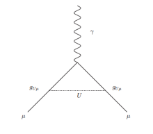
Figure 1: Feynman diagram contribution of $U$ to $g-2$ anomaly of $\mu$

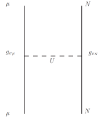
Figure 2: Feynman diagram contribution of $U$ to the Lamb shift anomaly of muonic hydrogen and deuterium

2 The $g-2$ and Lamb shift anomalies

As worked out in, for example [17], the state $H_{+}$ of present interest mixes at tree-level with the standard electroweak theory Higgs $h_{W}$ and with another state in the “hidden sector” called $H_{3}$ via the mass-squared submatrix:

$$M=\pmatrix{4\lambda_{W}\zeta_{W}^{2}&2\zeta_{W}\zeta_{S}(\nu_{1}-\nu_{2})\sqrt{\frac{1+2R}{3}}&2\sqrt{2}\zeta_{W}\zeta_{S}\nu_{1}\sqrt{\frac{1-R}{3}}\cr\ast&4(\kappa_{S}+\lambda_{S})\zeta_{S}^{2}\left(\frac{1+2R}{3}\right)&4\sqrt{2}\lambda_{S}\zeta_{S}^{2}\frac{\sqrt{(1+2R)(1-R)}}{3}\cr\ast&\ast&4(\kappa_{S}+2\lambda_{S})\zeta_{S}^{2}\left(\frac{1-R}{3}\right)\cr},$$ (9)

where the asterisks $\ast$ denote symmetric entries, $\lambda_{W},\lambda_{S},\kappa_{S},\nu_{1},\nu_{2}$ are coupling coefficients of various terms in the scalar framon self-interaction potential, $\zeta_{W}$ is the vacuum expectation value of the flavour framon (in other words, the electroweak Higgs field), and $\zeta_{S}$ the vacuum expectation value of its colour analogue. Of these quantities, which may all depend on scale, one knows at present only the values of $\lambda_{W},\zeta_{W}$ and an estimate for $\zeta_{S}$ at $\mu\sim m_{Z}$, and little about the scale-dependence of any.

An exception is the combination $R=\nu_{2}\zeta_{W}^{2}/2\kappa_{S}\zeta_{S}^{2}$ which occurs frequently in the FSM. It is a measure of the relative strength of the symmetry-breaking versus the symmetry-restoring terms in the framon potential for what is for quarks and leptons the generation symmetry, called $\widetilde{su}(3)$ in FSM. Its value and scale-dependence is correlated to that of the vector $\alpha$, the rotation of which with changing scale is what gives the hierarchical mass and mixing patterns of quarks and leptons, as mentioned in the Introduction. Thus the fit to these patterns [17] has already supplied us with the information of how $\alpha$, and hence also $R$ depend on scale. This is reproduced in Figures 3, 4 for easy future reference.

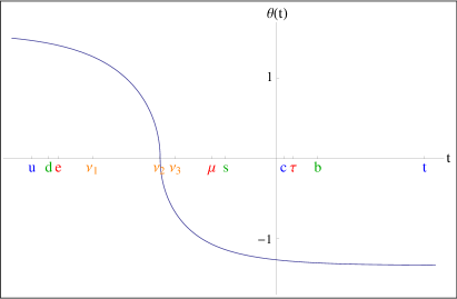
Figure 3: The polar angle $\theta$ of the normalized rotating vector $\alpha$ as a function of $t=\ln\mu$ ($\mu$ being the scale) obtained in [17] by fitting quark and lepton data, where the azimuthal angle $\phi$ is given by $\cos\theta\tan\phi=-0.1$

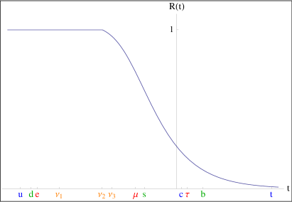
Figure 4: The ratio $R=\nu_{2}\zeta_{W}^{2}/2\kappa_{S}\zeta_{S}^{2}$ as a function of $t=\ln\mu$ ($\mu$ being the scale) obtained by the same fit to quark and lepton data in [17]

At tree level, were it not for the said mixing, $h_{W}$ would have the mass 125 GeV observed in experiment, $H_{3}$ would have a mass of order TeV [16, 19], and $H_{+}$ a mass of around 17 MeV, the same as its diagonal partners in $H_{\rm light}$ and $G_{\rm light}$, such as the $G_{3}$ or $X$ to be considered in Section 3 on the Atomki anomaly. The reason for such an abnormally small mass for these states is their having mass squared matrix elements proportional to $1-R$, as seen for example in (9), which, according to Figure 4, vanishes sharply at around 17 MeV and forces a solution near that value [17] to the condition:

$$m_{x}(\mu)=\mu$$ (10)

for the physical mass of any state $x$ by normal convention as a fixed point of the function $m_{x}(\mu)$.

When mixing by (9) is taken into account, the masses of all 3 states $h_{W},H_{3},H_{+}$ will change but are still expected to be close to the above values. In particular, the mixed state $U$ from $H_{+}$ would have a mass $m_{U}$ close to but above 17 MeV, say of order 20 MeV.

As to exactly how the mixing works out for (9), it is not as straightforward as it might seem at first sight. Since the parameters on which the matrix depends are themselves dependent on scale, some strongly such as $R$, and we are dealing with scales differing by some 5 orders in magnitude, it is unclear at what scale or scales that the matrix should be diagonalized. In our opinion, a stepwise diagonalization procedure, as adopted before for the rotating mass matrix in say [17], would seem appropriate. But we are unsure, not having in the “hidden sector” the same abundance of data to check against as in the earlier case in the standard sector. Besides, even if we just proceed as before, the answer will not be informative because the values of most parameters in (9) are still unknown or known only at certain scales.

Fortunately, for the problem at hand, little needs be known about the details of the mixing, so long as it is accepted that $U$ will acquire a component in $h_{W}$, say $\rho_{Uh}h_{W}$, where $\rho_{Uh}$ is presumably small which we can treat as an adjustable parameter to be fitted to experiment. We recall that $H_{+}$ has itself no direct couplings to quarks and leptons, so that $U$ will couple to quarks and leptons only via its $h_{W}$-component, and have thus the same couplings to these as $h_{W}$ does, only at a different scale and with strength reduced by the factor $\rho_{Uh}$.

The standard Higgs state $h_{W}$, in FSM as in SM, couples to quarks and leptons via the Yukawa term, but this term differs in details in the two models. In the SM, there is introduced a Yukawa term for each quark or lepton with a coupling proportional to the fermion mass. In the FSM, there is introduced only one Yukawa term for all three generations of each quark or lepton species, thus:

$$\sum_{[\tilde{a}],[\tilde{b}]}Y_{[\tilde{b}]}\bar{\psi}^{[\tilde{a}]}_{L}\alpha_{[\tilde{a}]}\phi\psi^{[\tilde{[b}]}_{R},$$ (11)

where the vector $\alpha$ is an attribute of the flavour framon which replaces the Higgs scalar field in the standard electroweak theory, and hence is independent of the species of quarks or leptons to which (11) refers.

Expanding (11) in fluctuations of the $h_{W}$ field about its vacuum expectation value $\zeta_{W}$, we obtain to zero-th order the mass matrix depending on the rotating vector $\alpha$, which gives in FSM the mass and mixing patterns of quarks and leptons mentioned in the Introduction . Then to first order,

$$\mathcal{L}_{Y}\,=\,-\sum_{T=U,D,L,\nu}\frac{m_{T}}{\zeta_{W}}\sum_{i=1,2,3}|\langle\mbox{\boldmath$\alpha$}(\mu)|f_{i}\rangle|^{2}\,\,\overline{f_{i}}{f_{i}}\,h_{W}.$$ (12)

In (12) then, only the coefficient $m_{T}$ depends on the species, this being the mass of the heaviest generation of that species, thus for the $U$-type quarks, $m_{T}=m_{t}$, the mass of the top quark, and for the charged leptons $m_{T}=m_{\tau}$, the mass of the tau lepton.

According to previous arguments then, the couplings of $U$ to quarks and leptons differ from (12) only by being multiplied by the mixing factor $\rho_{Uh}$ and by the fact that for the problems at hand the rotating scale-dependent vector $\alpha$ is to be evaluated, by usual prescription, at the scale of the $U$ mass, $m_{U}$.

The fit [17] to mass and mixing data for quarks and leptons has already supplied us with the information how $\alpha$ depends on scale $\mu$ as shown in Figure 3 from which $\mbox{\boldmath$\alpha$}(m_{U})$ can be read off. The same fit has also given us the state vectors $|f_{i}\rangle$ for all the quarks and leptons; in particular those for $\mu$, $e$ and $u$ which we shall need here are reproduced below for easy reference:

$$\langle\mu| = (0.07434,-0.53580,0.84107),$$

$$\langle e| = (0.42028,0.78168,0.46082),$$

$$\langle u| = (0.42041,0.53974,0.72934).$$ (13)

2.1 $g-2$

The contribution of Figure 1 to the $g-2$ anomaly $\Delta a_{\ell}$ is of the form [20]:

$$\Delta a_{l}\,=\,\frac{g_{U\ell}^{2}}{8\pi^{2}}\,\int_{0}^{1}dz\,\frac{(1+z)(1-z)^{2}}{(1-z)^{2}+z\left(\frac{m_{U}}{m_{\ell}}\right)^{2}}.$$ (14)

Given then the experimental bounds (1) on $\Delta a_{\mu}$, one obtains the corresponding bounds on $g_{U\mu}$ for any value we choose for $m_{U}$. We choose instead to display these bounds, using:

$$g_{U\ell}=\rho_{Uh}\frac{m_{\tau}}{\zeta_{W}}|\langle\mbox{\boldmath$\alpha$}(\mu)|\ell\rangle|^{2}$$ (15)

from (12), in terms of $\rho_{Uh}$, for easier comparison later with other channels, and obtain the result in Figure 5. One sees that in the expected range of $m_{U}$ around 20 MeV, $\rho_{Uh}$ is found to have value of order $10^{-1}$.

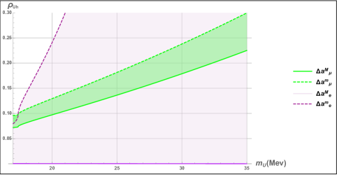
Figure 5: Experimental bounds on the mixing parameters $\rho_{Uh}$ from $g-2$ for muon (green) and electron (mauve), where the allowed regions are shaded

This conclusion can actually be deduced qualitatively without any explicit calculation as follows. For $m_{U}\sim 23$ MeV, and $m_{\mu}=105$ MeV, the $m_{U}$-dependent term in the integral in (14) is negligible so that the integral is of order unity and approximately constant. The quantity $|\langle\mu|\mbox{\boldmath$\alpha$}\rangle|^{2}m_{\tau}/\zeta_{W}$ in (15) has a value of order $3\times 10^{-3}$ , which gives immediately

$$\rho_{Uh}^{2}\sim 8\pi^{2}\times 10^{5}\times 10^{-9}\sim 10^{-2}$$ (16)

as claimed.

One notes here then a point:

• [n1] the value needed for $\rho_{Uh}$ is of order $10^{-1}$, (that is, $<1$ and small), which is consistent with its interpretation in FSM as a mixing parameter.

The experimental bound on $\Delta a_{e}$, we recall from (1), is some 3 orders lower than that for $\Delta a_{\mu}$. Most of this suppression is due just to kinematics, as seen in the integral (14), where now for $m_{U}\sim 23$ MeV and $m_{e}\sim 0.5$ MeV, and thus $m_{U}/m_{e}\sim 46$, the $m_{U}$-dependent term completely dominates, giving the integral approximately as $\sim(m_{e}/m_{U})^{2}\ln(m_{e}/m_{U})$, that is, already some 3 orders of magnitude lower. However, this is still not quite enough to satisfy the experimental bound which needs $g_{U\mu}>g_{Ue}$ by about another factor of around 3—6. And this is aptly supplied by the difference between $\langle e|\mbox{\boldmath$\alpha$}\rangle$ and $\langle\mu|\mbox{\boldmath$\alpha$}\rangle$ in (13) above. That this is so can of course be confirmed by detailed calculation as shown in Figure 5.

One notes then another point:

• [n2] For any value of $\rho_{Uh}$ allowed by experiment on the muon $g-2$ anomaly in the range of $m_{U}$ under consideration, the FSM predicts a value for the electron $g-2$ anomaly which automatically satisfies the bound set by experiment. This tests the FSM prescription in (15) for $U$ (and eventually (11) for $h_{W}$) for the relative sizes of the couplings to different generations of the same species (in this case the charged leptons).

2.2 Lamb Shift

The contribution of $U$ via Figure 2 to the splitting of the 2S-2P energy levels of leptonic atoms is given as [21]:

$$\delta E_{\ell}^{A}\,=\,-\,g_{U\ell}\,g_{UN}\,\frac{m_{U}^{2}a_{0N}}{8\pi\left(1+m_{U}a_{0N}\right)^{4}}$$ (17)

where $g_{UN}$ is the coupling of $U$ to the nucleus $N$, with mass $m_{N}$ and charge $Z$, of atom $A$ for which the Lamb shift is being considered, and

$$a_{0N}\,=\,\frac{1}{Z\alpha}\left(\frac{1}{m_{N}}+\frac{1}{m_{\ell}}\right)$$ (18)

is the Bohr radius, where $\alpha$ is the fine structure constant.

The formula (12) gives the $U$ couplings to quarks as:

$$g_{Uq}=\rho_{Uh}\frac{m_{t,b}}{\zeta_{W}}|\langle\mbox{\boldmath$\alpha$}(m_{U})|q\rangle|^{2}$$ (19)

which are similar in form to those to leptons in (15) except for the replacement of the factor $m_{\tau}$ by $m_{t}$ or $m_{b}$, depending on whether we are dealing with up-type or down-type quarks. To calculate $\delta E_{\ell}^{A}$ in (17), however, we need instead the $U$ couplings to the proton $p$ or possibly other nuclei. These we may write as:

$$g_{UN} = \rho_{Uh}\frac{m_{t}}{\zeta_{W}}\,\sum_{q=u,c,t}\langle N\mid\overline{q}q\,\mid N\rangle|\langle\mbox{\boldmath$\alpha$}(m_{U})|q\rangle|^{2}$$ (20)

$$+ \rho_{Uh}\frac{m_{b}}{\zeta_{W}}\,\sum_{q=d,s,b}\langle N\mid\overline{q}q\,\mid N\rangle|\langle\mbox{\boldmath$\alpha$}(m_{U})|q\rangle|^{2}.$$

Given that $m_{t}\gg m_{b}$, we can drop the second term which is some 2 orders down in magnitude. Furthermore, given that the nucleon or deuteron contains rather little $c\bar{c},t\bar{t}$, we can to a good approximation keep only one term in the sum of (20), and write:

$$g_{UN}\,=\,\rho_{Uh}\frac{m_{t}}{\zeta_{W}}\mid\langle\mbox{\boldmath$\alpha$}(m_{U})\mid u\rangle\mid^{2}\langle N|\overline{u}\,u\,|N\rangle.$$ (21)

That one can keep only the $u$ term in (20) is a great simplification specific to the FSM which will be seen to give explicit physical consequences.

To evaluate this, one needs the matrix element $\langle N|\overline{u}\,u\,|N\rangle$ involving nonperturbative physics, for which one has at present to rely on lattice calculations or on phenomenological methods. In Table 1 we list a sample selection we found in the literature giving rather different values for the matrix elements, reflecting presumably the uncertainty in the calculation.

Ref.	$\langle p|\bar{u}u|p\rangle$	$\langle n|\bar{u}u|n\rangle$	$\langle d|\bar{u}u|d\rangle$
(a)	2.10	1.31	3.38
(b)	2.8	2.2	—
(c)	5.2	4.3	—
(d)	6.8	6.0	—

Table 1: Relevant matrix elements at 2 GeV taken from lattice calculations (a) [22], (b) [23], (c) [24], and (d) phenomenological estimates [25]

With the matrix elements $\langle N|\bar{u}u|N\rangle$ taken from Table 1, divided by the factor 1.33 to take account of the running from 2 GeV to the nucleon mass scale at 1 GeV [26], one obtains then an estimate for the coupling $g_{UN}$. We shall take Reference (a) as benchmark, this being the only one to give an estimate for the deuteron and incidentally also the most recent, but the parallel results for cases (b), (c), and (d) can be readily inferred from those of (a).

Before we do so, however, we note first the following. One recalls from (5) that the value of $\delta E_{\mu}^{H}$ measured in experiment is about $-0.3$ meV. With all other quantities in the expression (17) already known, one can then estimate what sort of coupling $g_{Up}$ is needed to reproduce such a value for $\delta E_{\mu}^{H}$. The answer is that, rather surprisingly at first sight, $g_{Up}$ must be some 2 orders of magnitude larger than $g_{U\mu}$. That this is so can be seen as follows. The quantity $m_{U}a_{0N}$ in (17) for $m_{U}\sim$ 23 MeV has a value of about 33, so that:

$$\delta E_{\mu}^{H}\sim-g_{U\mu}g_{Up}(8\pi)^{-1}(33)^{-3}m_{U},$$ (22)

which works out as $g_{Up}\sim 3.0\times 10^{-2}$, a factor some 2 orders larger than $g_{U\mu}$ which is given by (21) as $4\times 10^{-4}$, as was claimed. This conclusion is obtained only from (17) and the data.

On the other hand, applying instead the formula (21) from FSM by the procedure outlined in the paragraph before last, one obtains the estimate $g_{Up}\sim 2.95\times 10^{-2}$, magically coinciding with the estimate above from data. The 2 orders of magnitude difference is aptly reproduced by the FSM in that the coupling $g_{Up}$ in (21) contains a factor $m_{t}$, in place of $m_{\tau}$ of the coupling $g_{U\mu}$ in (15), and indeed $m_{t}/m_{\tau}\sim 10^{2}$.

We note thus another point:

• [n3] To accommodate the experimental value for $\delta E_{\mu}^{H}$ in (5), the coupling $g_{Up}$ of $U$ to the proton has to be some two orders of magnitude greater than that to the muon $g_{U\mu}$, which is aptly reproduced by the FSM, because of $u$-dominance (21) and the fact that $m_{t}\gg m_{\tau}$. This checks near quantitatively the FSM prescription (12) for the $U$ (or $h_{W}$) couplings to fermions of different species (in this case the up-type quarks versus the charged leptons).

Next, we turn to the Lamb shift in muonic deuterium given in (5), where it is seen that $\delta E_{\mu}^{D}$ is less than twice that for muonic hydrogen $\delta E_{\mu}^{H}$, implying by (17) that

• [n4] the coupling $g_{Un}$ of $U$ to the neutron is less than that to the proton $g_{Up}$, and that this immediately follows from the FSM prediction (21) of dominance by the $u$ quark and that the neutron has less $u$ quarks than the proton. This checks again the FSM prescription (12) for $U$ (or $h_{W}$) couplings to different fermion species (this time up-type quarks versus down-type quarks).

The same analysis can be repeated for the electron to obtain the Lamb shift for ordinary hydrogen and deuterium. Again, given that the Bohr radii are here some 200 times larger than for muonic hydrogen and deuterium, the Lamb shifts are also appropriately suppressed, and these effects, together with the smaller $U$ couplings to the electron than to the muon, are enough to bring the anomaly below present experimental sensitivity. Hence

• [n2’] Given $\rho_{U\ell}$ in Figure 5, the FSM predicts values of the Lamb shift anomalies for the electron which are below present experimental detection sensitivity, as is indeed the case.

2.3 $g-2$ and Lamb shift combined

Inputting next the experimental bounds in (5) on $\delta E_{\mu}^{H}$, and using (17) and the formulae (15) and (21), one obtains, for (a) in Table 1, the bounds on $\rho_{Uh}$ displayed in Figure 6. The same is done with the Lamb shift in deuterium and shown together with the earlier bounds obtained from the $g-2$ anomaly. One notes that all three bands overlap in the range 23 - 29 MeV, which means that

• [n5] For all bounds on muonic $g-2$ and Lamb shift to be satisfied, $m_{U}$ has to be in the range 23 - 29 MeV, right in the region expected by (10).

Had one chosen to work with (b), (c) or (d) of Table 1 instead of (a), it would mean just parallely shifting the Lamb shift bands a little to the right to higher values in $m_{U}$, but still broadly in the expected range.

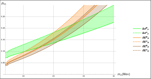
Figure 6: Experimental bounds on the mixing parameters $\rho_{Uh}$ from muonic $g-2$ (green), Lamb shift in muonic hydrogen (orange), and Lamb shift in muonic deterium (brown), where the allowed regions are shaded

It is interesting that in coming to the conclusion of a mass for $U$ of order 20 MeV in [n5], one has made no use of the mass condition (10) at all. The conclusion was drawn merely from the data on the two anomalies and the assumption that they both arise by virtue of the same $U$ boson. Then the requirement of consistency between the two sets of data already leads to the result $m_{U}\sim 20$ MeV. One may thus regard [n5] as an independent check by data on a qualitative prediction of the FSM.

Conversely, given that $m_{U}\sim 20$ MeV is already expected from (9) and (10), which assertion can in principle be confirmed in future when enough information on the parameters involved becomes available to allow the solution of (10), then the same result can be rephrased in summary of this section as:

• [n6] By adjusting a single free parameter $\rho_{Uh}$, the FSM has accommodated the following 6 independent pieces of experimental information:

  $$\Delta a_{\mu},\Delta a_{e},\delta E_{\mu}^{H},\delta E_{\mu}^{D},\delta E_{e}^{H},\delta E_{e}^{D},$$

  on two distinct physical effects, namely $g-2$ and Lamb shift, which need, a priori, have nothing to do with each other.

However, the above analysis, seemingly successful so far, has difficulty in explaining the apparent absence of a Lamb shift anomaly in some preliminary data on muonic helium [27, 28]. Also it gives mixed results when applied to bounds involving heavy nuclei:

• Nucleon binding energy in nuclear matter.

  $$\Delta B=\frac{1}{4m_{U}^{2}}\left(g_{Up}\,+\,g_{Un}\right)^{2}\rho$$ (23)

  $\rho=0.64\times 10^{6}$ MeV³. The experimental limit [28] is $\Delta B<1$ MeV.

• In neutron scattering on lead, the quantity to consider is (assuming coherence in the nuclear-scalar interaction) the effective coupling [29]:

  $$g_{Un}\left(\frac{A-Z}{A}g_{Un}\,+\,\frac{Z}{A}g_{Up}\right),$$

  where A = 208; Z = 82 for Pb. The experimental limit for this [30, 31] works out to be $5.6\times 10^{-10}\left(\frac{m_{U}}{\mathrm{MeV}}\right)^{4}$, giving the bounds, for $m_{U}=$ 23 MeV:

  $$g_{Up}\,<\,0.018,\quad g_{Un}\,<\,0.011,$$ (24)

The values obtained earlier in FSM, namely: $g_{Up}=0.030,g_{Un}=0.018$, pass the former bound giving $\Delta B\sim 0.6$, but exceed the latter bound by a factor of about 1.6. These are traditional difficulties for attempts to explain the Lamb shift anomaly by a new particle as the present case. To us, it points to some nonlinear effects which spoil the simple picture adopted above of the lepton interacting individually with the quark constituents. This might work to a certain extent in a nucleon, although, even there, one is troubled by uncertainties as indicated by the very different results listed in Table 1. But for a complex nucleus, such an approximation might become untenable. Indeed, even for the deuteron, one already begins to see some strain, noting the small overlap in Figure 6 between the hydrogen and deuterium bands, which, if the approximation works perfectly, should be identical. This seems to us to be a problem in nuclear physics to which we have at present no answer. Later on, in Section 3, we shall encounter another possible complication due to compound couplings of the $U$ to nucleons, which might interfere with the above couplings $g_{U_{p,n}}$ and further affect these bounds.

3 The Atomki anomaly

As already noted in the Introduction, the $U$ boson considered in the preceding section being scalar with $J^{P}=0^{+}$, cannot function as the anomaly $X$ in Atomki if parity and angular momentum are conserved. We switch our attention therefore to the vector state called $G_{3}$ in [16]. This $G_{3}$ is already diagonal at tree-level with mass squared eigenvalue $m_{3}^{2}=(g_{3}^{2}/6)(1-R)\zeta_{S}^{2}$, where $g_{3}$ is the colour gauge coupling, $\zeta_{S}$ the vacuum expectation value of the colour framon, and $R$ the scale-dependent ratio of couplings displayed in Figure 4. As for the $H_{+}$ or $U$ boson, the physical mass of $G_{3}$ is to be given by solving the fixed point equation (10). Recalling in Figure 4 that $1-R$ goes sharply to zero near $\mu=$ 17 MeV, and that $\zeta_{S}$ is bounded in [16] to have a value more than 2 TeV at scales of order $\mu\sim m_{Z}$, it follows that (10) for $G_{3}$ must have a solution very near to 17 MeV. There is here no complication due to mixing as there is in the parallel problem for $H_{+}$ above.

• [n7] In other words, the FSM at tree-level predicts quite precisely and with little ambiguity a physical mass for $G_{3}$ right on top of the anomaly at 17 MeV observed by Atomki.

Like the $H_{+}$, this $G_{3}$ belongs to the hidden sector in the FSM with no direct coupling to standard model particles, and acquires such couplings only via mixing. But in contrast to the $H_{+}$ which mixes with the standard sector already at tree level, $G_{3}$ mixes only at 1-loop level. According to [16] where the couplings of one $G$ to two $H$ are listed in Appendix B, both $G_{3}$ and $G_{8}$ are coupled to $H_{6},H_{7}$ (and also $H_{8},H_{9}$) so that $G_{3}$ can mix with $G_{8}$ via the loop displayed in Figure 7. There are no doubt similar mixing terms with loops of other particles. And since it has already been shown in [16, 19] that $G_{8}$ mixes with the photon $\gamma$ and with $Z$, it follows that this new mixing will induce a mixing of $G_{3}$ with $\gamma$ and $Z$ as well, acquiring for the mixed state $X$ some small couplings to quarks and leptons via $\gamma$ and $Z$, a fact that we wish now to demonstrate.

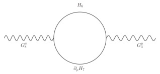
Figure 7: Sample 1-loop diagram mixing $G_{3}$ with $G_{8}$

In FSM, however, one is not yet in a position to evaluate loop diagrams in general, the technology for which has not yet been developed. One difficulty, as in the mixing of $U$ in the preceding section, is not knowing at what scale to do the calculation when faced with quantities which are strongly scale-dependent. One cannot therefore perform at present a fully consistent calculation to one loop. Our aim is only to indicate how the loop insertion in Figure 7 will lead to the mixing of $G_{3}$ and acquire for the mixed state $X$ a component in $\gamma$. And we shall take the loop contribution, which we cannot yet calculate, as a small adjustable parameter $\epsilon$ to be treated perturbatively.

The $4\times 4$ mass squared matrix for the whole $\gamma-Z-G_{8}-G_{3}$ complex then appears as:

$$H=H_{0}+H^{\prime},$$ (25)

with rows and columns labelled by $A_{\mu},\tilde{B}_{\mu}^{3},\tilde{C}_{\mu}^{8},\tilde{C}_{\mu}^{3}$ representing the relevant components of the various fields, where

$$H_{0}=\left(\begin{array}[]{cc}M&0\\ 0&m_{3}^{2}\end{array}\right),$$ (26)

and

$$H^{\prime}=\left(\begin{array}[]{cccc}0&0&0&0\\ 0&0&0&0\\ 0&0&0&\epsilon\\ 0&0&\epsilon&0\end{array}\right),$$ (27)

The top left $3\times 3$ block $M$ has already been diagonalized in [19, 16], giving $\gamma,Z,G$ as the eigenstates, corresponding to eigenvalues denoted $m_{\gamma}^{2}(=0),m_{Z}^{2},m_{G}^{2}$. First order perturbation theory for the perturbed $G_{3}$ state, now identified with $X$ in Atomki, then appears as:

$$\psi_{X}=u_{G_{3}}+\sum_{k=\gamma,Z,G}\frac{\langle k|H^{\prime}|G_{3}\rangle u_{k}}{m_{k}^{2}-m_{3}^{2}}.$$ (28)

In the equation above, $u_{j}$ is the unperturbed state vector of the $jth$ eigenstate in the original gauge basis $A_{\mu},\tilde{B}_{\mu}^{3},\tilde{C}_{\mu}^{8},\tilde{C}_{\mu}^{3}$. So $u_{G_{3}}$ is just $(0,0,0,1)$ which has no component in $A_{\mu}$ and $\tilde{B}_{\mu}^{3}$ and therefore no coupling to leptons and quarks. In the second term which represents the perturbation, the sum is completely dominated by the $k=\gamma$ term because of the denominator, since $m_{3}^{2}\sim(17\ {\rm MeV})^{2},m_{Z}^{2}\sim(100{\rm GeV})^{2},m_{G}^{2}\sim({\rm TeV})^{2}$. Hence,

$$\psi_{X}\sim u_{G3}-\frac{1}{m_{3}^{2}}\langle\gamma|H^{\prime}|G_{3}\rangle u_{\gamma}.$$ (29)

Now according to equation (28) of [19], the state vector $u_{\gamma}$ for $\gamma$ is

$$u_{\gamma}^{\dagger}=\left(\frac{e}{g_{1}},\frac{e}{g_{2}},\frac{2}{\sqrt{3}}\frac{e}{g_{3}},0\right).$$ (30)

Hence,

$$(\gamma|H^{\prime}|G_{3}) = u_{\gamma}^{\dagger}\left(\begin{array}[]{cccc}0&0&0&0\\ 0&0&0&0\\ 0&0&0&\epsilon\\ 0&0&\epsilon&0\end{array}\right)\left(\begin{array}[]{c}0\\ 0\\ 0\\ 1\end{array}\right)$$ (39)

$$= u_{\gamma}^{\dagger}\left(\begin{array}[]{c}0\\ 0\\ \epsilon\\ 0\end{array}\right)$$ (44)

$$= \frac{2e}{\sqrt{3}g_{3}}\epsilon.$$ (45)

This shows that the state $\psi_{X}$ in (29) has indeed acquired a component in $\gamma$ as anticipated.

Finally the factor $u_{\gamma}$ at the end of (29) ensures that it couples to quarks and leptons like the photon, except that the coupling is reduced by the mixing parameter factor $\rho_{X\gamma}=\frac{2e}{\sqrt{3}g_{3}}\frac{\epsilon}{m_{3}^{2}}$. In this respect, therefore, it behaves as what is often called in the literature a dark photon, and as far as the leptons are concerned, it seems that is all we need at present. Thus, it follows for example that $X$ can decay into $e^{+}e^{-}$ pairs as is seen in Atomki.

However, $X$ is not just a dark photon, since it is mainly $G_{3}$, and $G_{3}$ is not a fundamental field in the FSM but a bound state of a colour framon-antiframon pair in $p$-wave bound by colour confinement, as interpreted following the confinement picture of ’t Hooft [18]. To know how it interacts with the nucleons in the beryllium nucleus, which are also composite states bound by colour confinement, seems thus a rather complicated affair, probably involving nonperturbative effects, a problem one is not in a position to deal with at present, nor perhaps for some time to come. We propose therefore to treat the coupling of $G_{3}$ or $X$ to nucleons as a parameter, say $\kappa_{p}$ or $\kappa_{n}$, which would be almost the same except that the dark photon-like couplings deduced before for charged quarks would still be there and give an extra bit to the proton though not to the neutron. But the difference appears to be small compared to the parameter itself, as we shall see later.

In that case, the analysis given in [32] applies and gives an estimate for the ratio of interest:

$$\frac{\Gamma({}^{8}{\rm Be}^{*}\rightarrow{}^{8}{\rm Be}+(X\rightarrow e^{+}e^{-}))}{\Gamma({}^{8}{\rm Be}^{*}\rightarrow{}^{8}{\rm Be}+\gamma)} \sim \frac{(\kappa_{p}+\kappa_{n})^{2}}{e^{2}}S_{K}{\rm BR}(X\rightarrow e^{+}e^{-})$$ (46)

$$\sim 5.8\times 10^{-6},$$

where $S_{K}$ is a kinematic suppression factor to account for the mass of the $X$ produced:

$$S_{K}=\left[1-\left(\frac{m_{X}}{18.15\ {\rm MeV}}\right)^{2}\right]^{3/2}.$$ (47)

One obtains thus the estimate:

$$\frac{|\kappa_{p}+\kappa_{n}|}{e}\ \sqrt{{\rm BR}}\sim 1.16\times 10^{-2}$$ (48)

or roughly:

$$\kappa_{p}\sim\kappa_{n}\sim 1.7\times 10^{-3}/\sqrt{{\rm BR}}.$$ (49)

In other words, when treating the $\kappa$ as parameters, there would be no difficulty in fitting the Atomki signal as it appears in experiment.

The question, however, is whether this interpetation of the Atomki anomaly as $X$ in FSM would satisfy the contraints set by other experiments, which is always the main problem in interpetations of the Atomki anomaly, as so clearly analysed in the two excellent reviews [32, 33] on the subject. In Table 2 are displayed the constraints listed in these reviews.

No.	Experiment	Bound	Estimate	OK?
$1^{\#}$	Møller scattering	$C_{eV}C_{eA}<10^{-8}$	$\sim 0$	OK
	SLAC E158
$2^{\#}$	Atomic parity	$-\frac{2\sqrt{2}}{G_{F}}C_{eA}$	$\sim 0$	OK
	violation in	$[C_{uV}(2Z+N)+C_{dV}(Z+2N)]$
	cesium	$\times\frac{0.8}{(17\ {\rm MeV})^{2}}<0.7$
$3^{*\#}$	$\nu-e$ scattering	$|C_{e}C_{\nu}|^{1/2}<10^{-4}$	$\sim 0$	OK
	TEXONO
$4^{*}$	$\nu$-nucleus	$|C_{\nu}C_{n}|^{1/2}<2\times 10^{-4}$	$\sim 0$	OK
	scattering
$5^{*\#}$	$e$ beam dump	$|C_{e}|>6\times 10^{-5}\times\sqrt{{\rm BR}}$	$\sim 3\times 10^{-4}$	OK
	SLAC E141
$6^{\#}$	$e$ beam dump	$|C_{e}|>1.3\times 10^{-4}\times\sqrt{{\rm BR}}$	$\sim 3\times 10^{-4}$	OK
	CERN NA64
$7^{*}$	$\eta\eta^{\prime}\rightarrow\gamma(X\rightarrow e^{+}e^{-})$	$|C_{e}|>6\times 10^{-6}\times\sqrt{{\rm BR}}$	$\sim 3\times 10^{-4}$	OK
	CERN CHARM
$8^{*\#}$	$e^{+}e^{-}$ formation	$|C_{e}|<6\times 10^{-3}/\sqrt{{\rm BR}}$	$\sim 3\times 10^{-4}$	OK
	KLOE-2
$9^{*\#}$	$g-2$ of electron	$|C_{e}|<5\times 10^{-4}$	$\sim 3\times 10^{-4}$	OK
$10^{*}$	neutron-lead	$|\kappa_{n}|<6.0\times 10^{-3}$	$1.7\times 10^{-3}/\sqrt{{\rm BR}}$	OK
	scattering
$11^{*\#}$	$\pi^{0}\rightarrow\gamma(X\rightarrow e^{+}e^{-})$	(a) $\!|2C_{uV}\!+\!C_{dV}|<3.6\!\times\!10^{-4}/\sqrt{{\rm BR}}$	$\sim 3\times 10^{-4}$	OK
	CERN NA48/2	(b) $\!|\kappa_{\pi}|<10^{-3}/\sqrt{{\rm BR}}$	none known	?

Table 2: Constraints taken from the reviews [32, 33] of Feng et al. (*) and Delle Rose et al. (#), in the notation of (#) for the $X$’s couplings, where for simplicity we write $C_{x}=(C_{xV}^{2}+C_{xA}^{2})^{1/2},x=e,\nu,n$, and BR stands for ${\rm BR}(X\to e^{+}e^{-})$. Since our $X$ couples almost exclusively to leptons like a dark photon, it has practically no coupling to neutrinos and no $C_{A}$, so that 1—4 are automatically satisfied. The fit to the Atomki signal gives no constraint on $C_{eV}$, so that one is free to choose $C_{eV}\sim 3\times 10^{-4}$ to satisfy both the lower bounds 5, 6, 7 and the upper bounds 8, 9. For the 2 remaining constraints, 10 on $\kappa_{n}$ is satisfied (conditionally—see text), while 11 is partly on (a) $|2C_{uV}+C_{dV}|$, which is satifsfied, and partly on (b) $\kappa_{\pi}$ for which no estimate is yet known so no conclusion can yet be drawn.

Note that in fitting the size of the Atomki signal only $|\kappa_{p}+\kappa_{n}|$ is involved; the coupling of $X$ to leptons is not constrained, which remains just dark photonic. Thus:

• [n8] $X$ acquires via mixing a component in $\gamma$, coupling thus to quarks and leptons like a dark photon, hence:

  • (i) It can decay into $e^{+}e^{-}$,

  • (ii) It has almost no coupling to $\nu$ and almost no axial coupling $C_{A}$ (which couplings would come only from the negligible $Z$ component), thus satisfying constraints 1—4 in Table 2,

  • (iii) Its coupling to the electron is constrained by 5—9 in Table 2 to have value $\sim 3\times 10^{-4}$ which is small compared with $\kappa_{p,n}$ in (49), thus contributing but little to its production in beryllium decay.

However,

• [n9] $X$ is not just a dark photon but a compound state bound by colour confinement. Hence,

  • it has additional compound couplings $\kappa_{p,n}$ which dominate $X$ production in $Be$ decay,

  • yet, as will be shown immediately below, it satisfies constraint 10 (conditionally) and 11 (a), and by-passes constraint 11 (b) in Table 2.

Consider first the constraint 10 from neutron-lead scattering on $\kappa_{n}$. Taking $\kappa_{n}\sim\kappa_{p}$ (since $C_{p}$ is small compared to $\kappa$), one obtains from (48) the estimate $\kappa_{n}\sim 1.7\times 10^{-3}/\sqrt{{\rm BR}}$, which is seen to satsify the constraint 10, provided ${\rm BR}={\rm BR}(X\to e^{+}e^{-})$ is not too small, as it is believed not to be (see [R6] in the next section). As for constraint 11, this is more complex, receiving contributions as it does from both the dark photonic and compound couplings of the $X$ to the pion. The constraint (a) given in [32, 33] is obtained by putting the compound coupling $\kappa_{\pi}$ of $X$ to the pion to $0$, which constraint is seen in Table 2 to be satisfied. Further, when the contributions of $\kappa_{\pi}$ is added, this constraint may have to be weakened, because of possible destructive interference between the two contributions, and continues therefore to be satisfied. A constraint (b) is implied, however, also on $\kappa_{\pi}$, but no estimate for this is yet known, so no conclusion can as yet be drawn whether this constraint is satified or not. Estimates have indeed been obtained before for the compound couplings of $X$ to nucleons $\kappa_{p,n}$. But it is not obvious how a bound on $\kappa_{\pi}$ will translate (if at all) into bounds on $\kappa_{p}$ or $\kappa_{n}$, to fathom which one would have to understand the mechanism how the fundamental couplings of gluons, framons and quarks give rise to the effective couplings $\kappa$ connecting the compound state $G_{3}$ to the other compound states $p,n$ or $\pi$. Thus, this constraint 11 which is the most restrictive to other models seems avoided by the present interpretation.

It is the fact that the $X$ in FSM is a composite state bound by colour confinement and so has a different interaction to hadrons than just that due to the dark photonic coupling to quark constituents, thus separating the leptonic couplings $C_{eV}$ and so on from the hadronic couplings $\kappa_{p,n}$, which allows the two sets of bounds 5-9 and 10-11 in Table 2 to be individually satisfied and keeps the present accommodation apparently consistent.

In addition, this interpetation of the Atomki anomaly is seen to be consistent with the interpretation of the $g-2$ and Lamb shift anomalies as $U$ in the preceding section. We recall that the $X$ boson here can in principle contribute to $g-2$ and Lamb shift as well but was neglected there because, we argued, the couplings of $X$ to leptons being of 1-loop order should be small compared to the leptonic couplings of $U$ which occur already at tree level. This checks with the numbers obtained above:

• [n10] The mixing parameter $\rho_{X\gamma}=C_{e}/e$ (that is, the $\gamma$-component of $X$) of order $10^{-3}$ is much smaller than $\rho_{Uh}$ of order $10^{-1}$, which is consistent with the FSM conception of $\rho_{Uh}$ being of tree-level and $\rho_{X\gamma}$ of 1-loop order.

Further, the couplings $\kappa_{p,n}$ of $X$ to nucleons should have equivalents for $U$ as well, both being composites bound by colour confinement, but in the analysis of the $g-2$ and Lamb shift anomalies in Section 2, such couplings were ignored, the couplings of $U$ to nucleons there being deduced only from the $U$ couplings to the constituent quarks. Whence then the difference? Again, it is because the dark photonic couplings of $X$ are of 1-loop order while the dark Higgs-like couplings of the $U$ occur at tree level. Hence, $C_{qV}\sim C_{eV}\sim 3\times 10^{-4}$ are smaller than the compound couplings to the nucleons $\kappa_{p,n}\sim 1.7\times 10^{-3}$ which dominate. On the other hand, for $U$, it would be the other way round, with the dark Higgs-like couplings dominating over the compound couplings. Hence the difference, namely,

• [n11] The compound coupling $\kappa_{p,n}$ being of order $2\times 10^{-3}$ is small compared with $g_{Up}$ of order $3\times 10^{-2}$. A parallel compound coupling for $U$ can thus reasonably be neglected at first instance, as it was in Section 2.

Indeed, we think that compound couplings of $U$ to hadrons similar to the compound couplings $\kappa_{p,n}$ for $X$ very likely exist (See also [R4] of Section 4), making the $U$ couplings to hadrons more complicated than the way they were pictured in Section 2, as we already hinted at the end of that section. This may not be too serious for the nucleon so that the analysis there still largely applies. But when dealing with heavier nuclei, it is possible that the complication multiplies and helps further to explain why we had difficulty with Lamb shift for helium and with neutron-lead scattering.

4 Concluding remarks

It might have been premature trying to accommodate experimental anomalies not yet fully established to a barely nascent theory with only limited predictive power but the attempt, it seems, has resulted in strengthened credibility and benefits for both. We note in particular the following salient points.

• [R1] A first bizarre feature of the anomalies when considered as new particles is their abnormally small couplings to leptons, and probably also to quarks. This fact has now found a possible explanation in the FSM in that the model predicts a hidden sector of particles with no direct coupling to those in the standard sector, but some of them, such as the scalar boson $H_{+}$ and the vector boson $G_{3}$, can acquire small couplings to quarks and leptons via mixing, the former with the standard Higgs boson $h_{W}$, and the latter with the photon. As listed in [n1], [n8], and [n10], the fitted values of the various couplings are consistent with their being such mixing parameters.

  Assigning the weakness of the anomalous signals to the smallness of mixing between a standard and a hidden sector, as the FSM does and as bourne out by the above analysis, has given the anomalies a very different significance to that obtained by assigning the same to the smallness of their couplings per se. The latter would make of the anomalies a sort of appendix to the standard sector which one may choose to ignore at first instance. But the former would make them both samples of and windows into a vast portion of our universe which has so far been hidden from us, a portion as complex and vibrant in itself as the portion we know and probably even weightier, as the amount of dark matter suggests. And this we can hardly neglect.

  On the other hand, although the existence of a sector of particles with no direct coupling to the standard ones, and that some among them, in particular $H_{+}$ and $G_{3}$, should acquire small couplings to quarks and leptons via mixing is a consequence of the FSM action, that the new sector should therefore be “hidden” depends on the assertion that these particles have none (or at least very little) of the soft interactions that hadrons have, despite the two types of particles having some similarity, both being compound states bound by colour confinement. This conclusion was arrived at based on two parallel arguments:

  • (i) by analogy [15] to the Higgs scalar $h_{W}$ and the vector bosons $W^{\pm},Z$ in the standard electroweak theory when this is pictured as a confined theory in the manner suggested by ’t Hooft [18],

  • (ii) by an intuitive argument [16] based on the observation that the framon constituents of the particles in the hidden sector have short lifetimes.

  Neither the analogy nor the intuitive argument, however, need be considered conclusive.

  Therefore, some phenomeological support for the validity of this “hiddenness” assertion in FSM would be welcome, and this seems now to be afforded by the anomalies as here interpreted. Indeed, if the anomalies are real and are interpreted as particles, then these particles cannot have the strong soft interactions that hadrons have, or else they would have been produced copiously and recognized a long time ago. Now, the only reminder one has of soft interaction in the above analysis is what we call the compound couplings $\kappa_{p,n}$ of the $X$ to nucleons in Section 3, and these we note are very small. One can thus regard this fact as an experimental check on the validity of the above assertion that particles in the hidden sector have little soft interactions with particles in the standard sector.

• [R2] A second bizarre feature of the anomalies interpreted as particles is their mass of around 20 MeV, a mass region which does not play any particular role in anything else we know. But it has found now an apparently natural home in the FSM, a model constructed originally, we recall, not for the anomalies but to address the generation puzzle in quarks and leptons. Indeed, new particles in this mass range were predicted by the FSM before they were thought to have anything to do with the anomalies, as noted already in [n5] and [n7], and this coincidence has added to their credibility.

  However, this FSM prediction is itself in need of some scrutiny. It was based on the following premises [16]

  • (i) That the physical mass of a particle $x$ is to be given by a solution of the fixed point equation (10), as applied above to $U$ and $X$, where $m_{x}(\mu)$ is its scale-dependent mass eigenvalue.

  • (ii) That $m_{x}(\mu)$ for the particles of present interest is as given by the fit to quark and lepton data reported in [17], going sharply to zero at around 17 MeV as seen in Figure 4.

  • (iii) That if there are two solutions to (10), then one takes the lower for the physical mass, the higher state being taken to be unstable against decay into the lower state.

  Although (i) is generally accepted, and (ii) and (iii) already applied in the earlier fit [17] to quarks and leptons with apparent success, so that a mass prediction of aroung 20 MeV for $U$ and $X$ is no more than pushing the above to its logical conclusion, it is still an audacious conclusion to draw, predicting particles in this mass range in a system the natural scale for which would seem to be of order TeV. But, as noted in [n5] and [n7] in the preceding sections, experiments do seem to support this conclusion. Thus, if both the anomalies and their present FSM interpetation are sustained, it would be a long shot which seems to have hit the mark and a major boost in the credibility of the logical process followed. It suggests also the possibility of a deeper significance to the scale of around 20 MeV than is apparent at present [34].

• [R3] Next, we turn to details. In the $g-2$ and Lamb shift anomalies interpreted as due to $U$ boson exchange, we have noted in the $U$ couplings the following pattern:

  • $g_{U\mu}>g_{Ue}$,

  • $g_{Up}\gg g_{U\mu}$,

  • $g_{Up}>g_{Un}$.

  As noted already in [n2], [n2’], [n3], [n4], this pattern is very well explained by the FSM, lending support again to the validity of the result.

  As far as the FSM is concerned, this pattern comes about from the Yukawa term (11), which we have noted already is different from that of the standard model, and is thus something that one would like to check carefully against experiment. The Yukawa coupling for FSM was constructed originally with the view of explaining the hierarchical mass and mixing patterns of quarks and leptons observed in experiment, which it did reasonably well [17]. However, to achieve this, use has been made only of the value of the Yukawa coupling taken at the vacuum expectation value of the Higgs scalar (or flavour framon) field. To test the model further, one would wish to ask whether this Yukawa coupling continues to hold even where the scalar field is away from, or fluctuates about, its vacuum expectation value. This means comparing the couplings of the Higgs boson with other particles to experiment. And this will be checking the implications of the Yukawa term (11) beyond the purpose for which it was originally constructed, or in other words, checking genuine predictions of the FSM scheme.

  One example for such a check would be the decay rates of the Higgs boson $h_{W}$ to quark and lepton pairs [35, 36] which works out in FSM to be:

  $$\Gamma(h_{W}\rightarrow\bar{f}_{i}f_{i})\propto m_{T}^{2}|{\bf f}_{i}\cdot\mbox{\boldmath$\alpha$}|^{4}$$ (50)

  where $\alpha$ is the rotating vector taken at the scale $\mu=m_{h}$, and ${\bf f}_{i}$ is the state vector of the quark or lepton state $f_{i}$, both of which are vectors in 3-D generation space. This prediction is very different from that of the standard model, namely $\Gamma(h\rightarrow\bar{f}_{i}f_{i})\propto m_{f_{i}}^{2}$. For the heaviest generation in each species the two models differ little numerically in their predictions, since at high scales, the rotation of $\alpha$ is slow and $m_{T}$ are just the masses of the heaviest generations, and these predictions check well with experiment. For the second generation, however, the FSM via (50) predicts generally much lower rates compared to those predicted by the SM. These differences can in principle be tested at the LHC. Unfortunatley the two most favourable cases for rates: $h\rightarrow\bar{c}{c},\bar{s}{s}$, are both heavily beset with background problems for detection, while the $\bar{\mu}\mu$ case which is not so beset has such a small rate that no events has yet been seen [16]. For these reasons, these checks with Higgs decays are not as yet practicable.

  However, we now note that the analyses of the $g-2$ and Lamb shift anomalies in Section 2 have in fact supplied us with an equally detailed check on the Yukawa term (11) to that afforded by Higgs decay, though at a much lower scale and admittedly less direct. In accommodating the anomalies, one has already checked, as one has hoped to do in Higgs decay, the predictions of the FSM Yukawa term for the couplings of $h_{W}$ to leptons and quarks not only for different generations of the same species in [n2] [n2’] but also the couplings to quarks and leptons of different species in [n3], [n4]. And here, besides, one has to run the vector $\alpha$ several orders of magnitude down in scale to order 20 MeV according to Figure 4 obtained earlier in [17], in effect making use of and testing the full armoury of the FSM prescriptions. It is in fact quite surprising that the prescriptions seem still so far to hold good.

  Had one adopted instead of (11) the SM Yukawa term where the couplings of $h_{W}$ to quarks and leptons of various species, and of various generations of each species, are just proportional to the mass of that particular quark or lepton, one would have obtained, for the $U$ couplings, still $g_{U\mu}>g_{Ue}$, but $g_{Uu}\ll g_{U\mu}$ and $g_{Uu}<g_{Ud}$, which in the same analysis would imply $g_{Up}\ll g_{U\mu}$ and $g_{Up}<g_{Un}$, that is, vastly at variance with the pattern noted above from experiment. But there is of course no reason for such a replacement. The SM has no call to explain the $U$ couplings since it predicts no $U$ particle mixing with $h_{W}$, while in the FSM, the Yukawa term (11) is part and parcel of the development in [16, 17] which predicted the $U$ in the first place, and cannot therefore be arbitrarily replaced.

Apart from the preceding examples of benefits going both ways, there are also some points where the above accommodation of the anomalies in experiment sheds some more light on the FSM hidden sector and serves to settle some ambiguities in the theory.

• [R4] Two high mass states $H_{\rm high}$ and $H_{\rm low}$ thought earlier in [16] to be metastable and possibly detectable in experiment now appear in view of the analysis in Section 2 to be highly unstable against decay into $U$.

• [R5] That $G_{3}$ or $X$ should have additional compound couplings $\kappa$ to hadrons other than those it acquires through its dark photonic couplings to quarks is a notion seemingly invented for the occasion to accommodate the Atomki anomaly in FSM, but actually it has already been envisaged before in [16] in a different context. Because of the very short framon life-time, it was argued there that framon bound states like $G_{3}$ or $X$ would be point-like and reluctant to engage in soft interactions. But it was also noted that this suppression of soft interactions is not absolute, not being due to a selection rule but only to a lack of probability. Indeed, it was even suggested there (in Section 10) that residual soft interaction may be responsible for the decay of some charged states of high mass which are unwanted as remnants in the present universe. Could then the compound couplings $\kappa$ introduced here in Section 3 be identified with the residual soft interactions envisaged there? Both are concerned with the situation when such a framonic bound state, which otherwise appears pointlike, enters an environment as obtains inside a hadron where colour is deconfined. Will such a state bound by colour confinement partly dissolve in such an environment, giving rise to the compound couplings $\kappa$ or the suggested residual soft interactions? If so, then the unwanted high mass charged members of the hidden sector which worried us in [16] can decay by emitting, for example, a charged pion to a low mass and stable neutral member of the hidden sector, and be removed as remnants of our present universe. Indeed, the value of $\kappa$ estimated by fitting the production rate of $X$ in Atomki in Section 3 would even give us then an estimate for their decay rate. The question is certainly food for thought and may in future figure as an important ingredient in FSM, not just in the decay of the high mass charged states just mentioned, but also in the interaction rates of other particles in the hidden sector which may function as constituents of dark matter. It might even suggest new ways of detecting dark matter particles.

• [R6] In the FSM, there is a colour analogue to the Yukawa coupling for the standard Higgs field (11), an analogue not easy to construct explicity, since the fermion field content is not yet completely known. There is thus a question whether some colour analogues of neutrinos, called co-neutrinos in [16], could acquire a very low mass via a see-saw mechanism similar to that suggested for neutrinos, giving them a mass low enough for the $H_{\rm light}$ and $G_{\rm light}$ mentioned in the Introduction to decay into, making these bosons unstable and thus excluded as dark matter candidates. In view of the suggestion, however, that $G_{3}$, a member of $G_{\rm light}$, is now identified as the Atomki anomaly $X$, this possibility becomes highly unlikely. The branching ratio ${\rm BR}(X\rightarrow e^{+}e^{-})$, given the estimate (49), is bounded by the constraint 10 in Table 2 to be not less than about 10 %, while if there is a light co-neutrino, then the decay rate into a pair of these will be enormous in comparison, given that the coupling of $G_{3}$ to co-neutrinos will be the colour gauge coupling $g_{3}$ . Therefore, if the identification of $G_{3}$ to $X$ is accepted, then there will likely be a bosonic component to dark matter as represented by the partners $G_{1,2}$ of $G_{3}$ in $G_{\rm light}$. These $G_{1,2}$ have no mixing with the standard sector as $G_{3}$ has, and so cannot decay into $e^{+}e^{-}$ as $X$ does, and having now also no light co-neutrinos to decay into, will seem stable and possible consituents of dark matter. Similarly, so will the partners of $U$ or $H_{+}$ in $H_{\rm light}$.

For these and other more obvious reasons, experimental confirmation of all the 3 anomalies are eagerly awaited.

References

-
[1]
G. W. Bennett et al. [Muon g-2 Collaboration], Phys. Rev. D73, 072003 (2006);
doi:10.1103/PhysRevD.73.072003; arXiv:hep-ex/0602035. -
[2]
F. Jegerlehner, A. Nyeffeler, Phys. Rep. 477 (2009) 1-110.
doi:10.1016/j.physrep.2009.04.003; arXiv:0902.3360 [hep-ph].
F. Jegerlehner, EPJ Web of Conferences 166, 00022 (2018).
doi:10.1051/epjconf/201816600022; arXiv:1705.00263 [hep-ph]. -
[3]
A. Keshavarzi, D. Nomura and T. Teubner,
Phys. Rev. D 97, 114025 (2018).
doi:10.1103/PhysRevD.97.114025; arXiv:1802.02995 [hep-ph]. -
[4]
R. Bouchendira, P. Clade, S. Guellati-Khelifa, F. Nez, and F. Biraben,
Phys. Rev. Lett. 106, 080801 (2011).
doi:10.1103/PhysRevLett.106.080801; arXiv:1012.3627 [physics.atom-ph]. - [5] R. Pohl et al., Nature 466, 213 (2010), doi:10.1038/nature09250.
- [6] A. Antognini, et al., Science 339, 417 (2013), doi:10.1126/science.1230016 .
-
[7]
Julian J. Krauth, Marc Diepold, Beatrice Franke, Aldo Antognini, Franz Kottmann, Randolf Pohl,
Annals of Physics 366 (2016) 168.
doi:10.1016/j.aop.2015.12.006; arXiv:1506.01298 [physics.atom-ph]. -
[8]
C. G. Parthey et al., Phys. Rev. Lett. 104, 233001 (2010).
doi:10.1103/PhysRevLett.104.233001. -
[9]
Randolf Pohl, Ronald Gilman, Gerald A. Miller and Krzysztof Pachucki, Annu. Rev. Nucl. Part. Sci. 2013. 63:175–204.
doi:10.1146/annurev-nucl-102212-170627; arXiv:1301.0905 [physics.atom-ph]. -
[10]
P. J. Mohr, B. N. Taylor, D. B. Newell, Rev. Mod. Phys. 80 (2008) 633.
doi:10.1103/RevModPhys.80.633; arXiv:0801.0028 [physics.atom-ph]. -
[11]
U. D. Jentschura, S. Kotochigova, E.-O. Le Bigot, P. J. Mohr, B. N. Taylor,
Phys. Rev. Lett. 95 (2005) 163003.
doi:10.1103/PhysRevLett.95.163003; arXiv:physics/0604058 [physics.atom-ph]. -
[12]
I. Sick, Phys. Rev. C 90, 064002 (2014).
doi:10.1103/PhysRevC.90.064002; arXiv:1412.2603 [nucl-ex]. -
[13]
J. C. Bernauer et al., (A1 Collab.) Phys. Rev. Lett. 105:242001 (2010).
doi:10.1103/PhysRevLett.105.242001; arXiv:1007.5076 [nucl-ex]. -
[14]
A. J. Krasznahorkay et al., Phys. Rev. Lett. 116, 042501 (2016).
doi:10.1103/PhysRevLett.116.042501; arXiv:1504.01527[nucl-ex]. - [15] José Bordes, Chan Hong-Mo and Tsou Sheung Tsun, Int. J. Mod. Phys. A33 (2018) 1830034; doi:10.1142/S0217751X1830034X; arXiv:1812.05373.
- [16] José Bordes, Chan Hong-Mo and Tsou Sheung Tsun, Int. J. Mod. Phys. A33 (2018) 1850195; doi:10.1142/S0217751X18501956; arXiv:1806.08268.
- [17] José Bordes, Chan Hong-Mo and Tsou Sheung Tsun, Int. J. Mod. Phys. A30 (2015) 1550051; doi:10.1142/S0217751X15500517; arXiv:1410.8022.
- [18] G. ’t Hooft, Acta Phys. Austr., Suppl. 22, 531 (1980).
- [19] José Bordes, Chan Hong-Mo and Tsou Sheung Tsun, Int. J. Mod. Phys. A33 (2018), 1850190; doi:217751X18501907; arXiv:1806.08271.
- [20] See for example: Lepton Dipole Moments, Advanced Series on Directions in High Energy Physics, Vol. 20 Editors B Lee Roberts and William J Marciano, World Scientific Publishing 2010
-
[21]
See for example: David Tucker-Smith and Itay Yavin, Phys. Rev. D 83, 101702 (2011).
doi:10.1103/PhysRevD.83.101702; arXiv:1011.4922 [hep-ph]. -
[22]
E. Chang, Z. Davoudi, W. Detmold, A. S. Gambhir, K. Orginos, M. J. Savage, P. E. Shanahan, M. L. Wagman, and F. Winter (NPLQCD Collaboration),
Phys. Rev. Lett. 120, 152002 (2018).
doi:10.1103/PhysRevLett.120.152002; arXiv:1712.03221 [hep-lat]. -
[23]
A. Abdel-Rehim, C. Alexandrou, M. Constantinou, K. Hadjiyiannakou, K. Jansen, Ch. Kallidonis, G. Koutsou, and A. Vaquero Avilés-Casco,
Phys. Rev. Lett. 116, 252001 (2016).
doi:10.1103/PhysRevLett.116.252001; arXiv:1601.01624 [hep-lat]. -
[24]
C. Alexandrou, M. Constantinou, P. Dimopoulos, R. Frezzotti, K. Hadjiyiannakou, K. Jansen, C. Kallidonis, B. Kostrzewa, G. Koutsou, M. Mangin-Brinet, A. Vaquero Avilès-Casco, and U. Wenger,
Phys. Rev. D95, 114514 (2017); Erratum Phys. Rev. D 96, 099906 (2017).
doi:10.1103/PhysRevD.95.114514 ; arXiv:1703.08788 [hep-lat]. -
[25]
J. Ellis, N. Nagata and K. A. Olive, Eur. Phys. J. C (2018) 78: 569.
doi:10.1140/epjc/s10052-018-6047-y. F. Bishara, J. Brod, B. Grinstein and J. Zupan, J. High Energ. Phys. 1711 (2017) 59.
doi:10.1007/JHEP11(2017)059. arXiv:1707.06998 [hep-ph] . -
[26]
M. Tanabashi et al. (Particle Data Group), Phys. Rev. D 98, 030001
(2018).
doi:10.1103/PhysRevD.98.030001 -
[27]
A. Antognini et al., EPJ Web Conf. 113, 01006 (2016).
doi:10.1051/epjconf/201611301006. -
[28]
Yu-Sheng Liu, David McKeen, and Gerald A. Miller,
Phys. Rev. Lett. 117, 101801 (2016).
doi:10.1103/PhysRevLett.117.101801; arXiv:1605.04612 [hep-ph]. -
[29]
H. Leeb and Schmiedmayer, Phys. Rev. Lett. 68, 1472 (1992).
doi:10.1103/PhysRevLett.68.1472. -
[30]
R. Barbieri, T. E. O. Ericson, Phys. Lett. B57, 270 (1975).
doi:10.1016/0370-2693(89)91102-7. - [31] V. Barger, Cheng-Wei Chiang, Wai-Yee Keung, and D. Marfatia, Phys. Rev. Lett. 106, 153001; doi:10.1103/PhysRevLett.106.153001 (2011).
-
[32]
Jonathan L. Feng et al., Phys. Rev. D95, 035017 (2017).
doi:10.1103/PhysRevD.95.035017; arXiv:1608.03591. - [33] Luis Delle Rose, Shaaban Khalil, Simon J. D. King and Stefano Moretti, Front. in Phys. 7 (2019) 43; doi:10.3389/fphy.2019.00073; arXiv:1812.05497.
-
[34]
James Bjorken, private communication; see also the website
bjphysicsnotes.com - [35] José Bordes, Chan Hong-Mo and Tsou Sheung Tsun, Eur. Phys. J. C65; 537-542, 2010; doi:10.1140/epjc/s10052-009-1186-9; arXiv:0908.1750.
-
[36]
Michael J Baker and Tsou Sheung Tsun, Eur. Phys. J. C70; 1009, 2010.
doi:10.1140/epjc/s100052-010-1506-0; arXiv:1005.2676.