Exponential damping induced by random and realistic perturbations

Abstract

Given a quantum many-body system and the expectation-value dynamics of some operator, we study how this reference dynamics is altered due to a perturbation of the system’s Hamiltonian. Based on projection operator techniques, we unveil that if the perturbation exhibits a random-matrix structure in the eigenbasis of the unperturbed Hamiltonian, then this perturbation effectively leads to an exponential damping of the original dynamics. Employing a combination of dynamical quantum typicality and numerical linked cluster expansions, we demonstrate that our theoretical findings for random matrices can, in some cases, be relevant for the dynamics of realistic quantum many-body models as well. Specifically, we study the decay of current autocorrelation functions in spin-$1/2$ ladder systems, where the rungs of the ladder are treated as a perturbation to the otherwise uncoupled legs. We find a convincing agreement between the exact dynamics and the lowest-order prediction over a wide range of interchain couplings.

I Introduction

Understanding the dynamics of interacting quantum many-body systems is notoriously challenging. While their complexity grows exponentially in the number of degrees of freedom, the strong correlations between the constituents often prohibit any exact solution. Although much progress has been made due to the development of powerful numerical machinery Schollwoeck2011 and the advance of controlled experimental platforms Bloch2008 ; Langen2015 , the detection of general (i.e. universal) principles which underlie the emerging many-body dynamics is of fundamental importance Polkovnikov2011 . To this end, a remarkably successful strategy in the past has been the usage of random-matrix ensembles instead of treating the full many-body problem. Ranging back to the description of nuclei spectra Brody1981 and of quantum chaos in systems with classical counterparts Bohigas1984 , random-matrix theory also forms the backbone of the celebrated eigenstate thermalization hypothesis (ETH) Deutsch1991 ; Srednicki1994 ; Rigol2005 , which provides a microscopic explanation for the emergence of thermalization in isolated quantum systems. More recently, random-circuit models have led to new insights into the scrambling of information and the onset of hydrodynamic transport in quantum systems undergoing unitary time evolution Keyserlingk2018 ; Nahum2018 ; Khemani2018 .

Concerning the out-of-equilibrium dynamics of quantum many-body systems, a particularly intriguing question is how the expectation-value dynamics of some operator is altered if the system’s Hamiltonian is modified by a (small or strong) perturbation. Clearly, the effect of such a perturbation in a (integrable or chaotic) system can be manifold. In the context of prethermalization Berges2004 ; Moeckel2008 ; Bertini2015 ; Mori2018 ; Reimann2019 ; Mallayya2019 , the perturbation breaks a conservation law of the (usually integrable) reference Hamiltonian, leading to a separation of time scales, where the system stays close to some long-lived nonthermal state, before eventually giving in to its thermal fate at much longer times. Moreover, in the study of echo protocols, time-local perturbations have been shown to entail irreversible quantum dynamics Schmitt2018 , analogous to the butterfly effect in classical chaotic systems. Furthermore, the observation that some types of temporal relaxation, such as the exponential decay, are more common than others can be traced back to their enhanced stability against perturbations Knipschild2018 .

In this paper, we consider a closed quantum many-body system ${\cal H}_{0}$ which is affected by a perturbation ${\cal V}$, such that the total Hamiltonian takes on the form

$${\cal H}={\cal H}_{0}+\lambda{\cal V}\ ,$$ (1)

where $\lambda$ denotes the strength of the perturbation. Given the expectation-value dynamics of some operator ${\cal O}$ in the unperturbed system,

$$\langle{\cal O}(t)\rangle_{{\cal H}_{0}}=\text{Tr}[{\cal O}\rho(t)]\ ,$$ (2)

where $\rho(t)=e^{-i{\cal H}_{0}t}\rho(0)e^{i{\cal H}_{0}t}$ [and $\rho(0)$ is a mixed or pure out-of-equilibrium initial state], we explore the question how $\langle{\cal O}(t)\rangle_{{\cal H}_{0}}$ is altered due to the presence of the perturbation, i.e., if $\rho(0)$ now evolves with respect to the full Hamiltonian ${\cal H}$. Employing the time-convolutionless (TCL) projection operator method Chaturvedi1979 ; Breuer2007 , we unveil for the idealized case of ${\cal V}$ exhibiting a random-matrix structure in the eigenbasis of ${\cal H}_{0}$, that such a perturbation effectively leads to an exponential damping of the original dynamics (see also Dabelow2019 ; Nation2019 ),

$$\langle{\cal O}(t)\rangle=\langle{\cal O}(t)\rangle_{{\cal H}_{0}}e^{-\lambda^{2}\gamma t}\ ,$$ (3)

where the damping rate $\gamma$ depends on the microscopic properties of ${\cal H}_{0}$ and ${\cal V}$. In order to illustrate that our analytical findings for random matrices can indeed be relevant for the dynamics of realistic quantum many-body systems, we numerically study the decay of current autocorrelation functions in spin-1/2 ladder models, where the rungs of the ladder are treated as a perturbation to the otherwise uncoupled legs. Especially for small to intermediate values of the interchain coupling, we find a convincing agreement between the exact dynamics and the leading-order prediction.

This paper is structured as follows. In Sec. II, we discuss the TCL formalism and present an analytical derivation of Eq. (3) for the case of ${\cal V}$ having an ideal random-matrix structure in the eigenbasis of ${\cal H}_{0}$. Next, in Sec. III, we test the applicability of Eq. (3) by studying the real-time dynamics for more realistic models and perturbations using an efficient combination of dynamical quantum typicality and numerical linked cluster expansions. We summarize and conclude in Sec. IV.

II Projection operator approach to ideal random-matrix models

II.1 Derivation of the main result

Let us now derive Eq. (3) within the framework of the TCL projection operator technique. In the TCL formalism, the decomposition of the Hamiltonian (1) is usually done in such a way that the observable of interest (here the operator ${\cal O}$) is either conserved in the unperturbed system or only shows slow dynamics under evolution with ${\cal H}_{0}$. Moreover, in order to apply the TCL formalism, one needs to define a suitable projection operator ${\cal P}^{2}={\cal P}$, which projects onto the relevant degrees of freedom. For a comprehensive review, see, e.g., Chaturvedi1979 ; Breuer2007 .

In order to simplify the upcoming derivation, let us assume that ${\cal H}_{0}$ has a very high and almost uniform density of states

$$\Omega\approx 1/\Delta\omega\ ,$$ (4)

where $\Delta\omega$ is the mean level spacing. Moreover, we shift the true eigenvalues of ${\cal H}_{0}$ slightly, such that they result as $E_{\omega}=\Delta\omega\cdot\omega$, with $\omega$ being an integer. Although these conditions are not necessarily fulfilled for a given system, we expect corrections to our results to be irrelevant on time scales $t\ll 2\pi/\Delta\omega$.

To begin with, we define a Fourier component of the operator ${\cal O}$ in the eigenbasis of ${\cal H}_{0}$,

$${\cal O}_{\omega}=\frac{1}{\sqrt{z_{\omega}}}\sum_{\eta}\ket{\eta}{\cal O}_{\eta,\eta+\omega}\bra{\eta+\omega}+\text{h.c.}\ ,$$ (5)

with normalization $z_{\omega}=2\sum_{\eta}|{\cal O}_{\eta,\eta+\omega}|^{2}$, and construct a set of corresponding projection operators ${\cal P}_{\omega}$, which project onto the relevant part of the density matrix $\rho(t)$,

$${\cal P}_{\omega}\rho(t)=\text{Tr}[\rho(t){\cal O}_{\omega}]{\cal O}_{\omega}\ .$$ (6)

Note that, from the definition of ${\cal O}_{\omega}$, it immediately follows that

$$\langle{\cal O}(t)\rangle=\sum_{\omega}\sqrt{z_{\omega}}\langle{\cal O}_{\omega}(t)\rangle\ ,$$ (7)

which holds for any ${\cal H}$, and in the special case $\lambda=0$, we can further write

$$\langle{\cal O}(t)\rangle_{{\cal H}_{0}}=\sum_{\omega}\sqrt{z_{\omega}}\langle{\cal O}_{\omega}(0)\rangle\cos(\Delta\omega\cdot\omega t)\ .$$ (8)

In particular, the dynamics of ${\cal O}_{\omega}$ in the Schrödinger picture and in the interaction picture (subscript $I$) are related by

$$\text{Tr}[{\cal O}_{\omega}\rho(t)]=\text{Tr}[{\cal O}_{\omega}\rho_{I}(t)]\cos(\Delta\omega\cdot\omega t)\ .$$ (9)

Next, we focus on initial states $\rho(0)$, which fulfill ${\cal P}_{\omega}\rho(0)=\rho(0)$ Breuer2007 . For such initial states, the TCL framework then yields a time-local equation for ${\cal O}_{I,\omega}(t)=\text{Tr}[{\cal O}_{\omega}\rho_{I}(t)]$, comprising a systematic perturbation expansion in powers of $\lambda$ Breuer2007 ,

$$\dot{{\cal O}}_{I,\omega}(t)=-\gamma_{\omega}(t){\cal O}_{I,\omega}(t)\ ;\ \ \gamma_{\omega}(t)=\sum_{n}\lambda^{n}\gamma_{\omega,n}(t)\ ,$$ (10)

where the $\gamma_{\omega,n}(t)$ are time-dependent rates of $n$-th order. Due to our choice of the ${\cal P}_{\omega}$, all odd orders of this expansion vanish (as it is often the case in the TCL framework Breuer2007 ), and the leading-order term is

$$\gamma_{\omega,2}(t) =\int_{0}^{t}\text{d}t^{\prime}K_{\omega,2}(t^{\prime})\ ,$$ (11)

with

$$K_{\omega,2}(t)=\text{Tr}\left\{i[{\cal O}_{\omega},{\cal V}_{I}(t)]i[{\cal O}_{\omega},{\cal V}]\right\}\ ,$$ (12)

and ${\cal V}_{I}(t)=e^{i{\cal H}_{0}t}{\cal V}e^{-i{\cal H}_{0}t}$. Here, the second-order kernel can be rewritten as $K_{\omega,2}(t)={\widetilde{K}}_{\omega,2}(t)+{\widehat{K}}_{\omega,2}(t)$, with

$${\widetilde{K}}_{\omega,2}(t) =\text{Tr}\left[-{\cal O}_{\omega}{\cal V}_{I}(t){\cal O}_{\omega}{\cal V}-{\cal V}_{I}(t){\cal O}_{\omega}{\cal V}{\cal O}_{\omega}\right]\,,$$ (13)

$${\widehat{K}}_{\omega,2}(t) =\text{Tr}\left[{\cal O}_{\omega}{\cal V}_{I}(t){\cal V}{\cal O}_{\omega}+{\cal O}_{\omega}{\cal V}{\cal V}_{I}(t){\cal O}_{\omega}\right]\ .$$ (14)

Let us stress that we made no assumptions on the specific form of the perturbation ${\cal V}$ up to this point.

For the idealized case of ${\cal V}$ being an entirely random (and possibly banded) matrix in the eigenbasis of the unperturbed system ${\cal H}_{0}$, it is possible to derive an analytic expression for the leading-order rate $\gamma_{2}(t)$. Focusing on this case, the terms in (13) consist of sums in which each addend carries a product of two uncorrelated random numbers. If the random numbers have mean zero, these sums should be negligible,

$${\widetilde{K}}_{\omega,2}(t)\approx 0\ .$$ (15)

In contrast, the terms in (14) do contribute, and we find

$${\widehat{K}}_{\omega,2}(t) =\frac{4}{z_{\omega}}\sum_{\eta,\kappa}|{\cal V}_{\kappa,\eta}|^{2}|{\cal O}_{\eta,\eta+\omega}|^{2}\cos\left[(\kappa-\eta)\Delta\omega t\right]$$

$$\approx\frac{4\Omega\overline{v^{2}}}{z_{\omega}}\sum_{\eta}\int_{-W}^{W}|{\cal O}_{\eta,\eta+\omega}|^{2}\cos(\chi t)\,\text{d}\chi$$ (16)

$$=2\Omega\overline{v^{2}}\int_{-W}^{W}\cos(\chi t)\,\text{d}\chi=4\Omega\overline{v^{2}}\,\frac{\sin(Wt)}{t}\ .$$ (17)

Several comments are in order. Since ${\cal V}$ is a random matrix, we have approximated in Eq. (16) all squared individual matrix elements by their averages $\overline{v^{2}}$, i.e., $|{\cal V}_{\kappa,\eta}|^{2}\approx\overline{v^{2}}$. Furthermore, we have used an index shift $\kappa\to\chi+\eta$ and converted the original sum over $\kappa$ to an integral, where $W$ denotes the half-bandwidth of ${\cal V}$. From (16) to (17), we have exploited that sum and integral can be evaluated independently and used the definition of $z_{\omega}$. Inserting (17) into the definition of $\gamma_{\omega,2}(t)$ yields

$$\gamma_{\omega,2}(t)\approx 4\Omega\overline{v^{2}}\int_{0}^{t}\text{d}t^{\prime}\frac{\sin(Wt^{\prime})}{t^{\prime}}\approx 2\pi\Omega\overline{v^{2}}\ ,$$ (18)

for times $t\gg\pi/W$, and we abbreviate

$$\gamma=2\pi\Omega\overline{v^{2}}\ .$$ (19)

From the inspection of Eq. (10) it then follows that ${\cal O}_{I,\omega}(t)=\langle{\cal O}_{\omega}(0)\rangle e^{-\lambda^{2}\gamma t}$, and a transformation back to the Schrödinger picture yields our main result in Eq. (3). Note that $\gamma$ is of the very same form as a rate describing the transition out of an initially fully populated eigenstate $|\eta\rangle$ of ${\cal H}_{0}$, as induced by ${\cal V}$, calculated from Fermi’s Golden Rule.

II.2 Discussion of the main result

Let us discuss our main result (3) in some more detail. First, we note that Eq. (3) is consistent with very recent findings in Refs. Dabelow2019 ; Nation2019 , although the employed approaches to arrive at this result have been very different. While the approaches in Refs. Dabelow2019 ; Nation2019 rely heavily on the concept of the perturbations being effectively represented by random matrices, their results on dynamics technically address averages over ensembles of random matrices. However, either by relying on “self-averaging” Nation2019 or as the result of a detailed calculation Dabelow2019 , the outcome for a specific perturbation is expected to be very close to the ensemble average. On the contrary, since the present analysis is based on projection operator techniques, it is in principle applicable to any specific (matrix)form of the perturbation. The result of this technique is given as a perturbation series containing all orders of the interaction strength $\lambda$, cf. Eq. (10). However, even in leading order, the evaluation is in general rather involved.

Next, we note that our derivations within the TCL approach are rigorous for an idealized random perturbation ${\cal V}$ up to second order in the perturbation strength. This truncation relies on ${\cal V}^{2}$ being dominantly diagonal (in the eigenbasis of ${\cal H}_{0}$). Random matrices also, but not exclusively, exhibit this feature Bartsch2008 .

While we have derived Eq. (3) for an idealized model and perturbation, this does not necessarily exclude the possibility that this equation is relevant also beyond such idealized cases. For instance, the ETH assumes a (almost) random-matrix structure of physical operators in the eigenbasis of generic Hamiltonians Srednicki1994 ; Rigol2005 , as numerically verified for various models Beugeling2015 ; Mondaini2017 ; Richter2019_3 . In fact, in the upcoming Sec. III, we numerically illustrate that Eq. (3) is indeed also applicable to understand the dynamics of certain realistic quantum many-body systems and perturbations. In this context, let us add that the phenomenon of an exponential damping has been found for an even wider range of realistic models, for instance in Refs. Flesch2008 ; Trotzky2012 ; Barmettler2009 ; Balzer2015 .

Nevertheless, we should stress that for a given model and perturbation, it is a priori certainly questionable whether a unitary basis transformation of the (originally nonrandom) perturbation can indeed yield entirely uncorrelated matrix elements. One criterion to check whether or not our arguments for random matrices also hold for realistic models is the evaluation of higher-order corrections. For example, the fourth-order rate $\gamma_{4}(t)$ in the TCL formalism reads

$$\gamma_{4}(t) = \int_{0}^{t}\!\text{d}t_{1}\int_{0}^{t_{1}}\!\text{d}t_{2}\int_{0}^{t_{2}}\text{d}t_{3}$$

$$\!K_{2}(t-t_{1})\;K_{2}(t_{2}-t_{3})$$

$$+ \!K_{2}(t-t_{2})\;K_{2}(t_{1}-t_{3})$$

$$+ \!K_{2}(t-t_{3})\;K_{2}(t_{1}-t_{2})$$

$$- \!\text{Tr}\{[[{\cal O},{\cal V}_{I}(t_{1})],{\cal V}_{I}(t)]\,[[{\cal O},{\cal V}_{I}(t_{3})],{\cal V}_{I}(t_{2})]\}\,,$$

where we have dropped the subscript $\omega$ for simplicity. If one finds that $\gamma_{4}(t)$ is significantly smaller than $\gamma_{2}(t)$ on the time scale of relaxation, this could be interpreted as an indication that ${\cal V}$ (in the eigenbasis of ${\cal H}_{0}$) is sufficiently well describable by a (pseudo)random matrix. Note that, in practice, the (numerical or analytical) evaluation of Eq. (II.2) is considerably more difficult compared to the second-order rate in Eq. (12) Steinigeweg2013 .

While the detailed analysis of correlations between matrix elements is beyond the scope of the present paper, let us note that one can find various realistic models where $\gamma_{4}(t)\ll\gamma_{2}(t)$ Steinigeweg2011 , while there are naturally also other models where this property as well as Eq. (3) do not hold anymore. One simple example would be the case where observable and perturbation commute, i.e., $[{\cal O},{\cal V}]=0$, and the second-order rate $\gamma_{2}(t)$ vanishes exactly. Another example where our framework necessarily fails by construction would be given by reversing the roles of ${\cal H}_{0}$ and ${\cal H}$, i.e., by defining a new unperturbed Hamiltonian as ${\cal H}_{0}^{\prime}={\cal H}_{0}+\lambda{\cal V}$, which is then perturbed by ${\cal V}^{\prime}=-\lambda{\cal V}$ such that ${\cal H}^{\prime}={\cal H}_{0}$.

III Numerical Illustration for quantum many-body systems

Let us now numerically illustrate that our main result (3) can be relevant for the dynamics of realistic quantum many-body systems. First, in Sec. III.1, we introduce the specific model and observable under consideration. In Sec. III.2, we then discuss our numerical approach which is used to study the real-time dynamics of the unperturbed and the perturbed system in Secs. III.3 and III.5, respectively. Moreover, we comment on the matrix structure of the realistic perturbation in the eigenbasis of ${\cal H}_{0}$ in Sec. III.4.

III.1 Model and Observable

We study a (quasi-)one-dimensional spin-$1/2$ lattice model with ladder geometry Zotos2004 ; Jung2006 ; Znidaric2013 ; Karrasch2015 ; Steinigeweg2016 , where the rung part of the ladder is treated as a perturbation to the otherwise uncoupled legs, i.e., the Hamiltonian reads ${\cal H}=J_{\parallel}{\cal H}_{0}+J_{\perp}{\cal V}$, with

$${\cal H}_{0}=\sum_{l=1}^{L}\sum_{k=1}^{2}S_{l,k}^{x}S_{l+1,k}^{x}+S_{l,k}^{y}S_{l+1,k}^{y}+\Delta S_{l,k}^{z}S_{l+1,k}^{z}$$ (21)

and

$$\quad{\cal V}=\sum_{l=1}^{L}S_{l,1}^{x}S_{l,2}^{x}+S_{l,1}^{y}S_{l,2}^{y}+\Delta S_{l,1}^{z}S_{l,2}^{z}\ .$$ (22)

Here, ${\bf S}_{l,k}=(S_{l,k}^{x},S_{l,k}^{y},S_{l,k}^{z})$ are spin-$1/2$ operators, $J_{\parallel}$ ($J_{\perp})$ is the coupling constant on the legs (rungs), and $L$ denotes the length of the ladder. Moreover, the anisotropy $\Delta$ is chosen to be either $\Delta=0$ (XX ladder) or $\Delta=1$ (XXX ladder). While, for $J_{\perp}=0$, ${\cal H}$ consists of two separate chains and is integrable, this integrability is broken for any $J_{\perp}\neq 0$.

For this model, let us study the current autocorrelation function

$$C(t)=\frac{\langle j(t)j\rangle_{\text{eq}}}{L}=\frac{\text{Tr}[\rho_{\text{eq}}j(t)j]}{L}\ ,$$ (23)

where $\rho_{\text{eq}}=e^{-\beta{\cal H}}/{\cal Z}$ is the canonical density matrix, $\beta=1/T$ denotes the inverse temperature, and $j(t)=e^{i{\cal H}t}je^{-i{\cal H}t}$. Moreover, the spin-current operator $j$ follows from a lattice continuity equation Heidrichmeisner2007 , and is given by

$$j=J_{\parallel}\sum_{l=1}^{L}\sum_{k=1}^{2}(S_{l,k}^{x}S_{l+1,k}^{y}-S_{l,k}^{y}S_{l+1,k}^{x})\ .$$ (24)

(Note that $j$ is independent of the perturbation ${\cal V}$.) Specifically, we here focus on the case of infinite temperature $\beta=0$ ($\rho_{\text{eq}}=\mathbb{1}/4^{L}$), and the correlation function $C(t)$ can be interpreted as the expectation-value dynamics

$$C(t)=\langle j(t)\rangle=\text{Tr}[j\rho(t)]\ ,$$ (25)

resulting from an initial state

$$\rho(0)\propto\mathbb{1}+\varepsilon j\ ,\ \quad\text{Tr}[\rho(0)]=1\ ,$$ (26)

with $\varepsilon$ sufficiently small. Given the decomposition in Eqs. (21) and (22) and choosing a simple projection onto the current $j$,

$${\cal P}\rho(t)=\frac{1}{4^{L}}+\frac{\text{Tr}[j\rho(t)]}{\text{Tr}[j^{2}]}j\ ,$$ (27)

the TCL formalism can be readily applied to Eq. (25). As a consequence, the derivations outlined in Sec. II for the expectation-value dynamics $\langle{\cal O}(t)\rangle$ carry over to the high-temperature correlation function $C(t)$, which allows us to test whether or not our results for random matrices are relevant for this more realistic setting.

III.2 Numerical approach

The correlation function $C(t)$ is an important quantity in the context of transport. Despite the integrability of ${\cal H}_{0}$, the dynamics of $C(t)$ is nontrivial even for $J_{\perp}=0$ Bertini2020 . While $C(t)$ has been numerically studied by various methods Sirker2009 ; Karrasch2012 ; Karrasch2015 ; Richter2019_2 , we here rely on a combination of dynamical quantum typicality (DQT) Gemmer2004 ; Popescu2006 ; Goldstein2006 ; Reimann2007 ; Bartsch2009 ; Hams2000 ; Iitaka2003 ; Sugiura2013 ; Elsayed2013 ; Steinigeweg2014 ; Steinigeweg2015 and numerical linked cluster expansions (NLCE) Tang2013 ; Mallayya2018 , recently put forward by two of us Richter2019 .

III.2.1 Dynamical quantum typicality

On the one hand, the concept of DQT relies on the fact that a single pure quantum state can imitate the full statistical ensemble. Specifically, for $\beta=0$, $C(t)$ can be written as a scalar product with the two pure states Elsayed2013 ; Steinigeweg2014

$$\ket{\psi(t)} =e^{-i{\cal H}t}j\ket{\varphi}\ ,$$ (28)

$$\ket{\varphi(t)} =e^{-i{\cal H}t}\ket{\varphi}\ ,$$ (29)

according to

$$C(t)=\frac{\bra{\varphi(t)}j\ket{\psi(t)}}{L\braket{\varphi}{\varphi}}+\epsilon\ ,$$ (30)

where the reference pure state $\ket{\varphi}$ is randomly drawn (Haar measure Bartsch2009 ) from the full Hilbert space with dimension $D=4^{L}$. Importantly, the statistical error $\epsilon=\epsilon(\ket{\varphi})$ vanishes as $\epsilon\propto 1/\sqrt{D}$ (for $\beta=0$), and the approximation becomes very accurate already for moderate values of $L$. Since the time evolution of pure states can be conveniently evaluated by iteratively solving the Schrödinger equation, e.g., by means of fourth-order Runge-Kutta Elsayed2013 ; Steinigeweg2014 or Trotter decompositions deReadt2006 , it is possible to treat large $D$, out of reach for standard exact diagonalization (ED).

III.2.2 Numerical linked cluster expansion

On the other hand, NLCE provides a means to obtain $C(t)$ directly in the thermodynamic limit $L\to\infty$. Specifically, the current autocorrelation is calculated as the sum of contributions from all connected clusters which can be embedded on the lattice Tang2013 ,

$$\frac{\langle j(t)j\rangle_{\text{eq}}}{L}=\sum_{c}{\cal L}_{c}W_{c}(t)\ ,$$ (31)

where $W_{c}(t)$ is the weight of cluster $c$ with multiplicity ${\cal L}_{c}$. The notion of a cluster here refers to a finite number of lattice sites which are coupled by the respective Hamiltonian. In fact, for a one-dimensional chain geometry [and also a (quasi-)one-dimensional ladder system] the identification of clusters becomes very simple. Namely, clusters are just chains (or ladders) of finite length. More details can be found in Refs. Tang2013 ; Mallayya2018 ; Richter2019 . Moreover, since there is only one distinct cluster for a given cluster size, we have ${\cal L}_{c}=1$ in Eq. (31).

Given a cluster $c$, its weight $W_{c}(t)$ is obtained by the so-called inclusion-exclusion principle,

$$W_{c}(t)=\langle j(t)j\rangle_{\text{eq}}^{(c)}-\sum_{s\subset c}W_{s}(t)\ ,$$ (32)

where $\langle j(t)j\rangle_{\text{eq}}^{(c)}$ denotes the (extensive) current autocorrelation evaluated on the cluster $c$ (with open boundary conditions). Furthermore, the sum in Eq. (32) runs over the weights $W_{s}(t)$ of all subclusters $s$ of $c$. Recall that for the (quasi-)one-dimensional geometry considered here, all subclusters are again just chains or ladders of finite size and Eq. (32) can be organized rather easily.

Within the NLCE, the contribution of each cluster is evaluated numerically exact. Thus, in practice, the series in Eq. (31) has to be truncated to a maximum cluster size $c_{\text{max}}$ which remains computationally feasible. This truncation in turn leads to a breakdown of convergence of $C(t)$ at some time $\tau$, where a larger $c_{\text{max}}$ leads to a longer $\tau$, see also Richter2019 ; White2017 . Thanks to the combination of NLCE with DQT (cf. Sec. III.2.1 and Richter2019 ), we can evaluate $\langle j(t)j\rangle_{\text{eq}}^{(c)}$ on large clusters beyond the range of ED, and obtain $C(t)$ in the thermodynamic limit for rather long times.

Eventually, let us note that while we here focus on $\beta=0$, both DQT and NLCE allow for accurate calculations of $C(t)$ at $\beta>0$ as well Steinigeweg2014 ; Steinigeweg2015 ; Richter2019 .

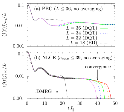
Figure 1: (Color online) (a) $C(t)$ for $J_{\perp}=0$ and $\Delta=1$ at $\beta=0$, obtained by ED ($L=18$) and DQT ($L\leq 39$) for PBC. $L$ here denotes the length of a single chain. (b) $C(t)$ obtained by NLCE up to expansion order $c_{\text{max}}\leq 39$. As a comparison, we depict tDMRG data Karrasch2015 .

III.3 Results for unperturbed dynamics

Now, let us study $C(t)$ in the unperturbed system ${\cal H}_{0}$. For vanishing anisotropy $\Delta=0$, the spin current $j$ is exactly conserved in the unperturbed system, $[{\cal H}_{0},j]=0$. As a consequence, we know the unperturbed dynamics for $\Delta=0$ exactly and only need to study the case $\Delta=1$ numerically, where ${\cal H}_{0}$ corresponds to two separate Heisenberg chains. In the remainder of Sec. III.3, we change the notation and denote by $L$ the length of a single chain (and not of the ladder).

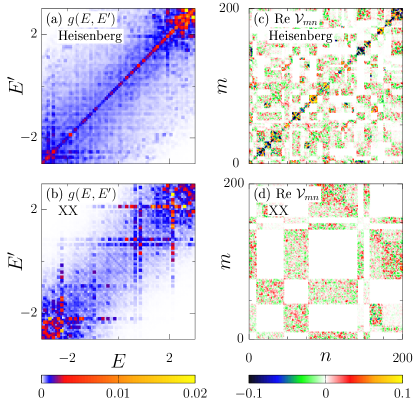
Figure 2: (Color online) Matrix structure of ${\cal V}$ in the eigenbasis of ${\cal H}_{0}$ in the symmetry subsector with magnetization $S^{z}=-1$, momentum $k=2\pi/L$, and even parity $p=1$, both for the Heisenberg ladder (top) and the XX ladder (bottom). The length of the ladder is $L=9$ in all cases.

In Fig. 1 (a), $\langle j(t)j\rangle_{\text{eq}}/L$ is shown for periodic boundary conditions (PBC), obtained by ED ($L=18$) and DQT ($L=32,34,36$) Steinigeweg2014 ; Richter2018 . While the curves for different $L$ coincide at short times, the ED curve starts to deviate from the DQT data for $t\gtrsim 8$. Moreover, for $t\gtrsim 20$, $C(t)$ takes on an approximately constant value which decreases with increasing $L$ Steinigeweg2014 .

Next, NLCE results for $C(t)$ are shown in Fig. 1 (b) for various expansion orders $c_{\text{max}}\leq 39$. For increasing $c_{\text{max}}$, we find that $C(t)$ is converged up to longer and longer times, until the expansion eventually breaks down. [Note that, for times above the convergence time, the data for $C(t)$ obtained by NLCE (i) has no physical meaning anymore and (ii) can for instance become negative, which leads to the discontinuity of the curves in the semilogarithmic plot used.] As a comparison, Fig. 1 (b) also shows data obtained by the time-dependent density matrix renormalization group (tDMRG) Karrasch2015 ; Kennes2016 . Apparently, tDMRG and NLCE agree perfectly for times $t\lesssim 27$. Moreover, for the largest $c_{\text{max}}=39$ considered by us, the NLCE data is converged up to times $t\approx 40$. This fact demonstrates that the combination of DQT and NLCE provides a powerful numerical approach to real-time correlation functions, and compared to Fig. 1 (a), also outperforms standard finite-size scaling on short to intermediate time scales.

Note that the determination of the unperturbed dynamics extends earlier results of Ref. Richter2019 and is an important building block of this paper in order to evaluate the prediction from the TCL formalism in Sec. III.5.

III.4 Matrix structure of the perturbation

Before discussing the real-time dynamics of $C(t)$ in the presence of ${\cal V}$, let us study the matrix structure of the realistic perturbation ${\cal V}$ from Eq. (22) in the eigenbasis of ${\cal H}_{0}$. To this end, we restrict ourselves to a single symmetry subsector with magnetization $S^{z}=-1$, momentum $k=2\pi/L$, and even parity $p=1$ to eliminate trivial symmetries. (Both ${\cal H}_{0}$ and ${\cal V}$ are entirely real in this case.)

First, we employ a suitable coarse graining according to Richter2019_3

$$g(E,E^{\prime})=\frac{\sum_{mn}|{\cal V}_{mn}|^{2}D(\bar{E})}{D(E)D(E^{\prime})}\,,$$ (33)

where the sum runs over matrix elements ${\cal V}_{mn}$ in two energy shells of width $2\delta E$, $E_{n}\in[E-\delta E,E+\delta E]$ and $E_{m}\in[E^{\prime}-\delta E,E^{\prime}+\delta E]$. $D(E)$, $D(E^{\prime})$, and $D(\bar{E})$ denote the number of states in these energy windows with mean energy $\bar{E}=(E+E^{\prime})/2$. In Figs. 2 (a) and (b), this coarse-grained structure of ${\cal V}$ is shown. Both for $\Delta=1$ and $\Delta=0$, we find that ${\cal V}$ is a banded matrix with more spectral weight close to the diagonal. However, especially in the case of the XX ladder, $g(E,E^{\prime})$ is not homogeneous within this band, but rather exhibits some fine structure.

For a more detailed analysis, a close-up of $200\times 200$ individual matrix elements ${\cal V}_{mn}$ is shown in Figs. 2 (c) and (d). We find that there is a coexistence between regions where the ${\cal V}_{mn}$ appear to be random, and regions where the ${\cal V}_{mn}$ vanish (e.g. due to additional conservation laws). Moreover, in the case of the XX ladder, these regions are more extended.

While it becomes obvious from Fig. 2 that the perturbation ${\cal V}$ is certainly not an entirely random matrix in the eigenbasis of ${\cal H}_{0}$ (which is also integrable such that the ETH is generally not expected to apply), we here refrain from a more detailed analysis of the residual correlations between the matrix elements. Nevertheless, given the overall banded structure of ${\cal V}$ and its apparent partial randomness, it is reasonable that our derivations from Sec. II can be relevant for this realistic model.

III.5 Comparison between perturbed dynamics and exponential damping

III.5.1 XX ladder

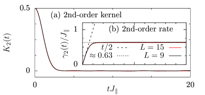
Figure 3: (Color online) (a) and (b) Second-order kernel $K_{2}(t)$ and decay rate $\gamma_{2}(t)$ for the XX ladder.

Next, we come to the actual discussion of $C(t)$ in spin ladders. ($L$ now denotes the length of the ladder.) Given the decomposition of ${\cal H}_{0}$ and ${\cal V}$ in Eq. (21) and the choice of the projector in Eq. (27), we can directly apply the TCL formalism to the decay of $C(t)$ in this model. First, we consider the case $\Delta=0$, i.e, the XX ladder. To start our analysis, we present in Figs. 3 (a) and (b) the second-order kernel $K_{2}(t)$,

$$K_{2}(t)=\frac{\text{Tr}\{i[j,{\cal V}_{I}(t)]i[j,{\cal V}]\}}{\text{Tr}\{j^{2}\}}\ .$$ (34)

Due to $[j,{\cal H}_{0}]=0$, or in cases where the dynamics in ${\cal H}_{0}$ is slow compared to the dynamics in ${\cal H}$ Steinigeweg2010 , this kernel simplifies to

$$K_{2}(t)=\frac{\text{Tr}\{i[j,{\cal V}_{I}](t)i[j,{\cal V}]\}}{\text{Tr}\{j^{2}\}}\ .$$ (35)

The corresponding decay rate $\gamma_{2}(t)$ reads,

$$\gamma_{2}(t)=\int_{0}^{t}\text{d}t^{\prime}K_{2}(t^{\prime})\ .$$ (36)

Comparing data for $L=9,15$, we observe that finite-size effects are negligible, and $\gamma_{2}(t)\approx 0.63$ becomes essentially constant for times $t\gtrsim 2$. Note that, since the XX chain can be brought into a quadratic form, $K_{2}(t)$ and $\gamma_{2}(t)$ could in principle even be obtained analytically for this particular case (see also Steinigeweg2011 ).

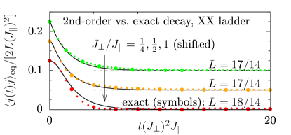
Figure 4: (Color online) $C(t)$ in XX ladders with several interchain couplings $J_{\perp}$ at $\beta=0$, obtained by DQT for two different $L\leq 18$ (small and large symbols). The curves indicate the second-order TCL prediction (37).

To proceed, Fig. 4 presents numerical data for the current autocorrelation function $C(t)$ for XX ladders with two different system sizes $L\leq 18$ and different coupling ratios $J_{\perp}/J_{\parallel}=1/4,1/2,1$ (symbols) Steinigeweg2014_2 , i.e., weak and strong values of the perturbation. Note that the data is vertically shifted for better visibility. Moreover, while the data is here obtained by DQT, we present NLCE data for the nonintegrable ladder model in Appendix B. As a comparison, the curves in Fig. 4 indicate our main result (3), i.e., the lowest-order prediction from the TCL formalism which reads

$$C(t)=C_{0}(t)\exp\left[-J_{\perp}^{2}\int_{0}^{t}\text{d}t^{\prime}\gamma_{2}(t^{\prime})\right]\ .$$ (37)

Recall that $j$ is exactly conserved in the unperturbed system, i.e., $C_{0}(t)=\text{const}.$, and the decay of $C(t)$ is solely due to ${\cal V}$. In Eq. (37), we take into account the full time dependence of the damping rate $\gamma_{2}(t)$. Namely, due to the linear growth of $\gamma_{2}(t)$ at short times, Eq. (37) leads to a Gaussian damping for $t\lesssim 1$, and turns into a conventional exponential damping for longer $t$,

$$C(t)\propto\begin{cases}e^{-aJ_{\perp}^{2}t^{2}}&t\lesssim 1\\ e^{-bJ_{\perp}^{2}t}&t>1\end{cases}\ .$$ (38)

As an important result, we find that Eq. (37) describes the actual decay of $C(t)$ remarkably well, albeit the agreement is certainly better for smaller $J_{\perp}/J_{\parallel}$. In this context, let us emphasize that for time-dependent problems, a truncation to lowest order is in general (for nonrandom matrices) not meaningful, even if the perturbation is small. For small perturbations, the relevant time scales are long and higher orders can become relevant on these time scales. Thus, the good agreement in Fig. 4 confirms that our derivations in the context of Eq. (3) can be relevant also for realistic perturbations and quantum many-body systems. A more detailed comparison and discussion can be found further below in Sec. III.5.3.

III.5.2 XXX ladder

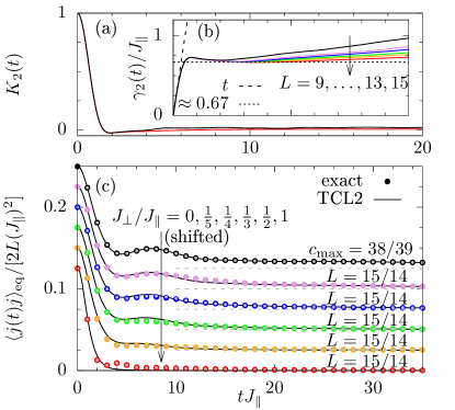
Figure 5: (Color online) (a) and (b) Analogous data as in Fig. 3, but now for the XXX ladder. (c) Analogous data as in Fig. 4, but now for the XXX ladder.

In order to corroborate our findings further, let us study another but similar model. Namely, we consider the dynamics of $C(t)$ for the case of $\Delta=1$, i.e., the XXX ladder.

The second order kernel $K_{2}(t)$ and the corresponding damping rate $\gamma_{2}(t)$ are shown in Figs. 5 (a) and (b) for various $L\leq 15$. Here, we again use for the kernel $K_{2}(t)$ the simplified version in Eq. (35), which is strictly valid for $[j,{\cal H}_{0}]=0$ only. Despite having $[j,{\cal H}_{0}]\neq 0$ in the case of the XXX ladder, it turns out that the finite-size scaling of this simplified form is much more favorable compared to the exact form in Eq. (34) (not depicted here) and, as discussed below, allows for an accurate description of the decay process.

Next, in Fig. 5 (c), the autocorrelation function $C(t)$ is shown for several values of the interchain coupling $J_{\perp}/J_{\parallel}=1/5,\dots,1$. We find that data for two different system sizes $L=14,15$ (symbols) nicely coincide with each other, i.e., at least on the time scales depicted trivial finite-size effect are negligible. This can be understood by, e.g., the onset of quantum chaos in the nonintegrable ladder and the smaller mean free path of spin excitations. (Additional NLCE data for the XXX ladder can be found in Appedix B.)

Analogous to our discussion in the context of Fig. 4, let us now compare this temporal decay of $C(t)$ to the prediction of an exponential damping. To this end, the unperturbed correlation function $C_{0}(t)$ is exponentially damped according to Eq. (37). Note that, as an important difference to the case $\Delta=0$, we now have a situation where the unperturbed dynamics $C_{0}(t)$ explicitly depends on time [see Fig. 1 (b)].

Similar to the case of the XX ladder, we find that Eq. (37) agrees very well with the exact $C(t)$ for all values of $J_{\perp}$ shown here, even when the perturbation is not weak. Let us stress that there is no free parameter involved.

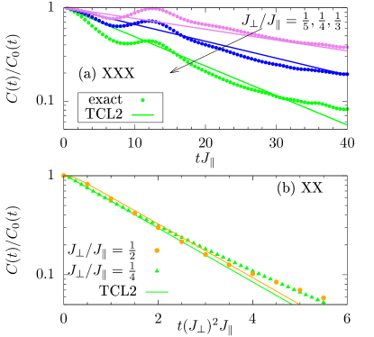
Figure 6: (Color online) Ratio $C(t)/C_{0}(t)$ between the autocorrelation function $C(t)$ in ladders with different $J_{\perp}$ and the unperturbed dynamics $C_{0}(t)$. The exact dynamics (symbols) is compared to the prediction from the second-order TCL formalism, cf. Eq. (37). (a) XXX ladder; (b) XX ladder.

III.5.3 Detailed analysis of agreement and discussion

Eventually, for a more detailed analysis, Fig. 6 shows the ratio $C(t)/C_{0}(t)$ between the perturbed and the unperturbed dynamics on a logarithmic scale, both for the XXX ladder [Fig. 6 (a)] and the XX ladder [Fig. 6 (b)]. Again, we compare the exact dynamics obtained by DQT and NLCE (symbols) to the prediction from the second-order TCL formalism (curves), i.e., the curves in Fig. 6 now represent the exponential damping term $\exp[-J_{\perp}^{2}\int_{0}^{t}\gamma_{2}(t^{\prime})\text{d}t^{\prime}]$.

For the XXX ladder, we find that while the exact dynamics exhibits some additional oscillations at intermediate times, the overall decay is convincingly captured by the TCL approach for the interchain couplings $J_{\perp}=1/5,1/4,1/3$ shown here. In particular for XX ladders with $J_{\perp}=1/4,1/2$, we find a very good agreement between the exact dynamics and the second-order prediction, at least for times $t(J_{\perp})^{2}\leq 4$.

Note that for time scales and coupling ratios beyond the ones shown in Fig. 6, especially in the long-time limit where finite-size effects still play a role, the agreement between the the lowest-order prediction and the exact dynamics becomes less convincing. Nevertheless, let us emphasize that for short to intermediate time scales (where most of the decay happens), an exponential damping is a convincing description of the relaxation dynamics of a perturbed quantum many-body systems.

IV Conclusion

How does the expectation-value dynamics of some operator changes under a perturbation of the system’s Hamiltonian? Based on projection operator techniques, we have answered this question for the case of a perturbation with random-matrix structure in the eigenbasis of the unperturbed Hamiltonian. As a main result, we have unveiled that such a (small) perturbation yields an exponential damping of the original reference dynamics, consistent with recent results in Refs. Dabelow2019 ; Nation2019 .

In addition, we have numerically confirmed that our findings can in some cases be readily applied to generic quantum many-body systems. Specifically, we have studied the decay of current autocorrelation functions in spin-$1/2$ ladder systems, where the rungs of the ladder are treated as a perturbation to the otherwise uncoupled legs. For this example, we have illustrated that even a truncation to second order in the perturbation still provides a convincing description of the main part of the decay process, also in cases where the perturbation is not weak.

While we have shown that for the specific spin-ladder model under consideration, the matrix representation of the perturbation ${\cal V}$ in the eigenbasis of ${\cal H}_{0}$ at least partially exhibits random segments, it is certainly questionable that realistic physical perturbations can be generally described by entirely random matrices. Therefore, a promising direction of future research includes the identification of relevant substructures, as well as a better understanding of the pertinent correlations between matrix elements Foini2019 .

Acknowledgments

This work has been funded by the Deutsche Forschungsgemeinschaft (DFG) - Grants No. 397107022 (GE 1657/3-1), No. 397067869 (STE 2243/3-1), No. 355031190 - within the DFG Research Unit FOR 2692. Additionally, we gratefully acknowledge the computing time, granted by the “JARA-HPC Vergabegremium” and provided on the “JARA-HPC Partition” part of the supercomputer “JUWELS” at Forschungszentrum Jülich.

Appendix A NLCE data for another integrable model

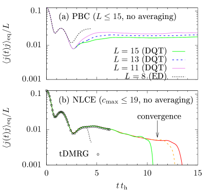
Figure 7: (Color online) (a) Current autocorrelation $C(t)$ in the Fermi-Hubbard chain ($U=4$), obtained by ED ($L=8$) and DQT ($L\leq 19$) at $\beta=0$ for periodic boundary conditions (PBC). (b) $C(t)$ obtained by NLCE up to expansion order $c_{\text{max}}\leq 19$. As a comparison, we depict data from the time-dependent density matrix renormalization group (tDMRG) Karrasch2014 .

In the main text, we have used a combination of DQT and NLCE to calculate the unperturbed dynamics of the spin-current autocorrelation function in the integrable spin-$1/2$ Heisenberg chain. This combination has allowed us to obtain numerically exact information on rather long time scales, which cannot be reached in direct calculations in systems with periodic or open boundary conditions, due to significant finite-size effects. To illustrate that this combination of DQT and NLCE can yield also for other integrable models the reference dynamics with a similar quality, we show additional data for the Fermi-Hubbard chain, described by the Hamiltonian ${\cal H}=\sum_{l=1}^{L}h_{l}$,

$$h_{l}=-t_{\text{h}}\sum_{s=\downarrow,\uparrow}(a_{l,s}^{\dagger}a_{l+1,s}+\text{H.c.})+U(n_{l,\downarrow}-\frac{1}{2})(n_{l,\uparrow}-\frac{1}{2})\,,$$ (39)

where the operator $a_{l,s}^{\dagger}$ ($a_{l,s}$) creates (annihilates) at site $l$ a fermion with spin $s$, $t_{\text{h}}$ is the hopping matrix element, and $L$ is the number of sites. The operator $n_{l,s}$ is the local occupation number and $U$ is the strength of the on-site interaction. For this model, we consider the particle current $j=\sum_{l=1}^{L}j_{l}$,

$$j_{l}=-t_{\text{h}}\sum_{s=\downarrow,\uparrow}(ia_{l,s}^{\dagger}a_{l+1,s}+\text{H.c.})\,,$$ (40)

and summarize our numerical results for the corresponding autocorrelation function with $U=4$ in Fig. 7. Apparently, the situation is like the one in Fig. 1 of the main text. On the one hand, in direct calculations with periodic boundary conditions, strong finite-size effects set in at short times, even for quite large $L$. On the other hand, NLCE for the largest expansion order $c_{\text{max}}$ is converged to substantially longer times. Even though not shown explicitly, we have checked that a good convergence is also reached for $U=8$. We thus expect that a perturbative analysis, as presented in this work, can be carried out for a wide class of quantum many-body systems, which we plan to do in detail in future work.

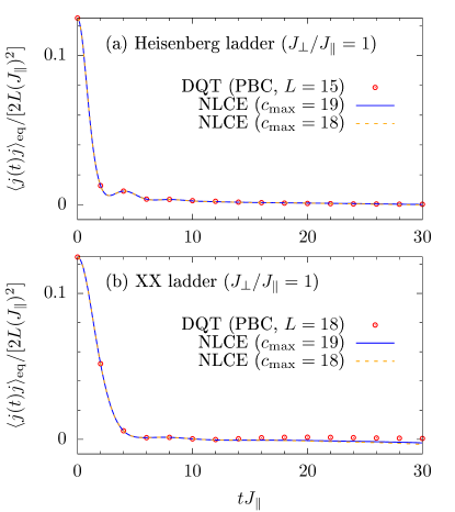
Figure 8: (Color online) Current autocorrelation $C(t)$ for the (a) Heisenberg ladder and (b) XX ladder, in both cases for $J_{\perp}/J_{\parallel}=1$. DQT data for periodic boundary conditions, as shown in the main text, is compared to NLCE data for two expansion orders $c_{\text{max}}=18$ and $19$.

Appendix B NLCE data for nonintegrable models

While it is certainly possible to use NLCE also for nonintegrable models, finite-size effects in direct calculations are much less pronounced in these models, as evident from Figs. 4 and 5 of the main text. This is why we have not shown corresponding NLCE data in these figures and instead relied on pure DQT data for systems with periodic boundary conditions. To demonstrate that these DQT data are indeed in excellent agreement with NLCE data, we show in Fig. 8 corresponding numerical results for the XXX and XX ladder, where we have chosen $J_{\perp}/J_{\parallel}=1$ in both cases.

References

- (1) U. Schollwöck, Ann. Phys. 326, 96 (2011).
- (2) I. Bloch, J. Dalibard, and W. Zwerger, Rev. Mod. Phys. 80, 885 (2008).
- (3) T. Langen, R. Geiger, and J. Schmiedmayer, Ann. Rev. Condens. Matter Phys. 6, 201 (2015).
- (4) A. Polkovnikov, K. Sengupta, A. Silva, and M. Vengalattore, Rev. Mod. Phys. 83, 863 (2011).
- (5) T. A. Brody, J. Flores, J. B. French, P. A. Mello, A. Pandey, and S. S. M. Wong, Rev. Mod. Phys. 53, 385 (1981).
- (6) O. Bohigas, M. J. Giannoni, and C. Schmit, Phys. Rev. Lett. 52, 1 (1984).
- (7) J. M. Deutsch, Phys. Rev. A 43, 2046 (1991).
- (8) M. Srednicki, Phys. Rev. E 50, 888 (1994).
- (9) M. Rigol, V. Dunjko, and M. Olshanii, Nature 452, 854 (2008).
- (10) C. W. von Keyserlingk, T. Rakovszky, F. Pollmann, and S. L. Sondhi, Phys. Rev. X 8, 021013 (2018).
- (11) A. Nahum, S. Vijay, and J. Haah, Phys. Rev. X 8, 021014 (2018).
- (12) V. Khemani, A. Vishwanath, and D. A. Huse, Phys. Rev. X 8, 031057 (2018).
- (13) J. Berges, Sz. Borsányi, and C. Wetterich, Phys. Rev. Lett. 93, 142002 (2004).
- (14) M. Moeckel and S. Kehrein, Phys. Rev. Lett. 100, 175702 (2008).
- (15) B. Bertini, F. H. L. Essler, S. Groha, and N. J. Robinson, Phys. Rev. Lett. 115, 180601 (2015).
- (16) T. Mori, T. N. Ikeda, E. Kaminishi, and M. Ueda, J. Phys. B 51, 112001 (2018).
- (17) P. Reimann and L. Dabelow, Phys. Rev. Lett. 122, 080603 (2019).
- (18) K. Mallayya, M. Rigol, and W. De Roeck, Phys. Rev. X 9, 021027 (2019).
- (19) M. Schmitt and S. Kehrein, Phys. Rev. B 98, 180301(R) (2018).
- (20) L. Knipschild and J. Gemmer, Phys. Rev. E 98, 062103 (2018).
- (21) S. Chaturvedi and F. Shibata, Z. Phys. B 35, 297 (1979).
- (22) H.-P. Breuer and F. Petruccione, The Theory of Open Quantum Systems (Oxford University Press, New York, 2007).
- (23) L. Dabelow and P. Reimann, Phys. Rev. Lett. 124, 120602 (2020).
- (24) C. Nation and D. Porras, Phys. Rev. E 99, 052139 (2019).
- (25) C. Bartsch, R. Steinigeweg, and J. Gemmer, Phys. Rev. E 77, 011119 (2008).
- (26) W. Beugeling, R. Moessner, and M. Haque, Phys. Rev. E 91, 012144 (2015).
- (27) R. Mondaini and M. Rigol, Phys. Rev. E 96, 012157 (2017).
- (28) J. Richter, J. Gemmer, and R. Steinigeweg, Phys. Rev. E 99, 050104(R) (2019).
- (29) A. Flesch, M. Cramer, I. P. McCulloch, U. Schollwöck, and J. Eisert, Phys. Rev. A 78, 033608 (2008).
- (30) S. Trotzky, Y-A. Chen, A. Flesch, I. P. McCulloch, U. Scholwöck, J. Eisert, and I. Bloch, Nat. Phys. 8, 325 (2012).
- (31) P. Barmettler, M. Punk, V. Gritsev, E. Demler, and E. Altman, Phys. Rev. Lett. 102, 130603 (2009).
- (32) K. Balzer, F. A. Wolf, I. P. McCulloch, P. Werner, and M. Eckstein, Phys. Rev. X 5, 031039 (2015).
- (33) R. Steinigeweg and T. Prosen, Phys. Rev. E 87, 050103(R) (2013).
- (34) R. Steinigeweg, Phys. Rev. E 84, 011136 (2011).
- (35) X. Zotos, Phys. Rev. Lett. 92, 067202 (2004).
- (36) P. Jung, R. W. Helmes, and A. Rosch, Phys. Rev. Lett. 96, 067202 (2006).
- (37) M. Žnidarič, Phys. Rev. B 88, 205135 (2013).
- (38) C. Karrasch, D. M. Kennes, and F. Heidrich-Meisner, Phys. Rev. B 91, 115130 (2015).
- (39) R. Steinigeweg, J. Herbrych, X. Zotos, and W. Brenig, Phys. Rev. Lett. 116, 017202 (2016).
- (40) F. Heidrich-Meisner, A. Honecker, and W. Brenig, Eur. Phys. J. Spec. Top. 151, 135 (2007).
- (41) B. Bertini, F. Heidrich-Meisner, C. Karrasch, T. Prosen, R. Steinigeweg, and M. Žnidarič, arXiv:2003.03334.
- (42) J. Sirker, R. G. Pereira, and I. Affleck, Phys. Rev. Lett. 103, 216602 (2009).
- (43) C. Karrasch, J. H. Bardarson, and J. E. Moore, Phys. Rev. Lett. 108, 227206 (2012).
- (44) J. Richter, F. Jin, L. Knipschild, J. Herbrych, H. De Raedt, K. Michielsen, J. Gemmer, and R. Steinigeweg, Phys. Rev. B 99, 144422 (2019).
- (45) J. Gemmer, M. Michel, and G. Mahler, Quantum Thermodynamics (Springer, Berlin, 2004).
- (46) S. Popescu, A. J. Short, and A. Winter, Nat. Phys. 2, 754 (2006).
- (47) S. Goldstein, J. L. Lebowitz, R. Tumulka, and N. Zanghì, Phys. Rev. Lett. 96, 050403 (2006).
- (48) P. Reimann, Phys. Rev. Lett. 99, 160404 (2007).
- (49) C. Bartsch and J. Gemmer, Phys. Rev. Lett. 102, 110403 (2009).
- (50) A. Hams and H. De Raedt, Phys. Rev. E 62, 4365 (2000).
- (51) T. Iitaka and T. Ebisuzaki, Phys. Rev. Lett. 90, 047203 (2003).
- (52) S. Sugiura and A. Shimizu, Phys. Rev. Lett. 111, 010401 (2013).
- (53) T. A. Elsayed and B. V. Fine, Phys. Rev. Lett. 110, 070404 (2013).
- (54) R. Steinigeweg, J. Gemmer, and W. Brenig, Phys. Rev. Lett. 112, 120601 (2014).
- (55) R. Steinigeweg, J. Gemmer, and W. Brenig, Phys. Rev. B 91, 104404 (2015).
- (56) B. Tang, E. Khatami, and M. Rigol, Comput. Phys. Commun. 184, 557 (2013).
- (57) K. Mallayya and M. Rigol, Phys. Rev. Lett. 120, 070603 (2018).
- (58) J. Richter and R. Steinigeweg, Phys. Rev. B 99, 094419 (2019).
- (59) H. De Raedt and K. Michielsen, in Handbook of Theoretical and Computational Nanotechnology (American Scientific Publishers, Los Angeles, 2006).
- (60) I. G. White, B. Sundar, and K. R. A. Hazzard, arXiv:1710.07696.
- (61) J. Richter, F. Jin, H. De Raedt, K. Michielsen, J. Gemmer, and R. Steinigeweg, Phys. Rev. B 97, 174430 (2018).
- (62) D. M. Kennes and C. Karrasch, Comput. Phys. Commun. 200, 37 (2016).
- (63) R. Steinigeweg and R. Schnalle, Phys. Rev. E 82, 040103(R) (2010).
- (64) R. Steinigeweg, F. Heidrich-Meisner, J. Gemmer, K. Michielsen, and H. De Raedt, Phys. Rev. B 90, 094417 (2014).
- (65) L. Foini and J. Kurchan, Phys. Rev. E 99, 042139 (2019).
- (66) C. Karrasch, D. M. Kennes, and J. E. Moore, Phys. Rev. B 90, 155104 (2014).