The Cost of a Reductions Approach to Private Fair Optimization

Abstract

Through the lens of information-theoretic reductions, we examine a reductions approach to fair optimization and learning where a black-box optimizer is used to learn a fair model for classification or regression. Quantifying the complexity, both statistically and computationally, of making such models satisfy the rigorous definition of differential privacy is our end goal. We resolve a few open questions and show applicability to fair machine learning, hypothesis testing, and to optimizing non-standard measures of classification loss. Furthermore, our sample complexity bounds are tight amongst all strategies that jointly minimize a composition of functions.

The reductions approach to fair optimization can be abstracted as the constrained group-objective optimization problem where we aim to optimize an objective that is a function of losses of individual groups, subject to some constraints. We give the first polynomial-time algorithms to solve the problem with $(\epsilon,0)$ or $(\epsilon,\delta)$ differential privacy guarantees when defined on a convex decision set (for example, the $\ell_{P}$ unit ball) with convex constraints and losses. Accompanying information-theoretic lower bounds for the problem are presented. In addition, compared to a previous method for ensuring differential privacy subject to a relaxed form of the equalized odds fairness constraint, the $(\epsilon,\delta)$-differentially private algorithm we present provides asymptotically better sample complexity guarantees, resulting in an exponential improvement in certain parameter regimes. We introduce a class of bounded divergence linear optimizers, which could be of independent interest, and specialize to pure and approximate differential privacy.

1 Introduction

Algorithmic fairness, accountability, and transparency of computer systems have become salient sub-fields of study within computer science. The incorporation of such values has led to the development of new models to make existing and state-of-the-art systems more conscious of societal constraints. But some of these new models do not adhere to other ethical standards. A standard of utmost importance is the need to ensure the privacy of the individuals that constitute the data used to create the models.

Differential privacy has become a gold standard of (individual-level) privacy in machine learning and data analysis (Dwork et al., 2006). The adoption of this privacy definition by the U.S. Census Bureau (Abowd, 2018) and major tech companies (Cormode et al., 2018) is evidence of its impact. Possibilities and implementations of reconstruction and inference attacks clearly show the relevance of differential privacy  (Dinur and Nissim, 2003; Consortium et al., 2009; Choromanski and Malkin, 2012; Shokri et al., 2017; Garfinkel et al., 2018; Carlini et al., 2019). Algorithmic fairness is also an increasingly important requirement for deployed systems, that results in various statistical tradeoffs (Kleinberg et al., 2017, 2020; Friedler et al., 2021). While the literature on differential privacy is guided by (slight variants of) a singular information-theoretic definition, the fairness literature is burgeoning without much clarity on what definitions are suitable for certain tasks. In this work, we provide a generic way to minimize group-fairness objectives by reducing to minimizing linear objectives. Given the worst-case nature of differential privacy, the best estimator for natural objectives – such as the least squares objective – depends on the properties of the dataset (Sheffet, 2019; Komarova and Nekipelov, 2020). As a consequence, the major advantage of the reductions approach is to use existing machinery for differentially private solvers to solve more general fairness objectives. However, what is the cost (both statistically and computationally) of this reductions approach? We aim to answer this question via the lens of information-theoretic reductions (Brassard et al., 1986; Bennett et al., 1995), using tools from Lagrangian Duality, Optimization, and Differential Privacy.

Our focus is on a reductions approach to fair optimization and learning where a black-box optimizer is used to learn a fair model for classification or regression ((Agarwal et al., 2018; Alabi et al., 2018)). We explore the creation of such fair models that adhere to differential privacy guarantees. This approach leads to applications other than algorithmic fairness. We consider two main suites of use cases: the first is for optimizing convex performance measures of the confusion matrix (such as those derived from the $G$-mean and $H$-mean); the second is for satisfying statistical definitions of algorithmic fairness (such as equalized odds, demographic parity, and the Gini index of inequality). See Section 8 for a few detailed generic examples of how to apply our results.

We abstract the reductions approach to fair optimization as the constrained group-objective optimization problem where we aim to optimize an objective that is a function of losses of individual groups, subject to some constraints. We present two differentially private algorithms: an $(\epsilon,0)$ exponential sampling algorithm and an $(\epsilon,\delta)$ algorithm that uses an approximate linear optimizer to incrementally move toward the best decision. The privacy and utility guarantees of these empirical risk minimization algorithms are presented. Compared to a previous method for ensuring differential privacy subject to a relaxed form of the equalized odds fairness constraint, the $(\epsilon,\delta)$-differentially private algorithm provides asymptotically better sample complexity guarantees. The technique of using a bounded divergence linear optimizer oracle to achieve strong guarantees of privacy/security and utility might be applicable to other problems not considered in this paper. Finally, we show an algorithm-agnostic information-theoretic lower bound on the excess risk (or equivalently, the sample complexity) of any solution to the problem of $(\epsilon,0)$ or $(\epsilon,\delta)$ private constrained group-objective optimization.

The focus of our work is on differentially private optimization via empirical risk minimization. Generalization guarantees can be obtained by taking a large enough sample of the population and of subgroups of the population. Another option is to consider the complexity (via VC dimension, for example) of the hypothesis class to be learned or the stability properties of the differentially private algorithms since we know that stability implies generalization (McAllester, 1999, 2003; Dwork et al., 2015; Feldman and Vondrák, 2019). We do not state any generalization guarantees in this paper but will motivate our work on empirical risk minimization in the context of the eventual goal of machine learning – generalization to unseen examples (Chervonenkis and Vapnik, 1971; Valiant, 1984; Littlestone, 1987; Blumer et al., 1989; Ehrenfeucht et al., 1989; Linial et al., 1991; Bousquet and Elisseeff, 2000; Koltchinskii and Panchenko, 2000; Vapnik, 2000; Zhang, 2006). The reason for this viewpoint and discussion is that differentially private algorithms exhibit (provable) stability properties that imply generalization. Our framework, via our notational and definitional setup, is amenable to analyses for stability properties.

Notation Setup and Example Usage

Suppose we have a dataset $D$ of size $n$ consisting of i.i.d. draws from an unknown distribution $\mathcal{D}$. For example, we could have $D=\{(\text{{x}}_{i},a_{i},y_{i})\}_{i=1}^{n}$ that consists of non-sensitive features $\text{{x}}_{1},\ldots,\text{{x}}_{n}\in\mathcal{X}$ of individuals, their corresponding sensitive attribute $a_{1},\ldots,a_{n}\in\mathcal{A}$, and their assigned labels/values (depending on if the resulting task is for classification, regression, etc.) $y_{1},\ldots,y_{n}\in\mathcal{Y}$. Let $\mathcal{C}_{P}$ be a decision set (e.g., corresponding to a set of $P$-dimensional decision vectors, a set of classifiers that each can be represented by $P$ real numbers, a set of all possible real coefficients of a polynomial threshold function, or a set of all possible weights that can be used to represent a specific neural network architecture) where $\mathcal{C}_{P}\subseteq\{c:(\mathcal{X}\times\mathcal{A})\rightarrow\mathcal{Y}\}$ or $\mathcal{C}_{P}\subseteq\{c:\mathcal{X}\rightarrow\mathcal{Y}\}$. We use $\mathcal{C}_{P}$ to mean that the decisions in $\mathcal{C}_{P}$ can be represented with at most $P$ real numbers whether $\mathcal{C}_{P}$ consists of classifiers or regression coefficient vectors. That is, the resulting parameter space lives in ${\mathbb{R}}^{P}$. For example, for a set of classifiers $\mathcal{C}_{P}$ consisting of single-dimensional thresholds, we have $\operatorname*{VC}(\mathcal{C}_{P})=P=1$. As another example, for $P>1$, let $L_{P}=\{c_{\text{{w}},b}~{}|~{}\text{{w}}\in{\mathbb{R}}^{P-1},b\in{\mathbb{R}}\}$ where $c_{\text{{w}},b}(\text{{x}})=\langle\text{{w}},\text{{x}}\rangle+b$. Then $L_{P}$ is parameterized by $\text{{w}}\in{\mathbb{R}}^{P-1},b\in{\mathbb{R}}$. For regression, $\mathcal{C}_{P}$ corresponds to the hypothesis class $L_{P}$ we wish to learn. For binary classification, $\mathcal{C}_{P}$ would correspond to the class of functions that result from the composition $\mathcal{C}_{P}=\operatorname*{sign}\circ~{}L_{P}$. For both the regression and classification problems in the aforementioned example, the hypotheses are parameterized by a $P$-dimensional vector. To apply differential privacy, it is important to know the hypothesis class we wish to learn since our statistical and computational guarantees must necessarily depend on properties of the class we wish to learn (De, 2012).

A goal could be to obtain a decision from $\mathcal{C}_{P}$ that can be used to classify an unseen $(\text{{x}}_{n+1},a_{n+1})\in(\mathcal{X}\times\mathcal{A})$ or $\text{{x}}_{n+1}\in\mathcal{X}$. Typically, the approach is to find a (provably optimal) predictor from the decision set $\mathcal{C}_{P}$ via empirical risk minimization and show that this predictor generalizes to unseen examples. Suppose there are at most $K$ groups to which any example $(\text{{x}},a,y)\sim\mathcal{D}$ can belong to. For any decision $c\in\mathcal{C}_{P}$, we define a loss function $\ell:\mathcal{C}_{P}\times(\mathcal{X}\times\mathcal{A}\times\mathcal{Y})^{n}\rightarrow[0,1]^{K}$ to be

$$\ell(c,D)=(\ell_{1}(c,D),\ldots,\ell_{K}(c,D)),$$

with $\ell_{k}(c,D)\in[0,1]$ for each $k\in[K]$. In addition, we also define the itemized (per example) loss function $\ell:\mathcal{C}_{P}\times(\mathcal{X}\times\mathcal{A}\times\mathcal{Y})\rightarrow[0,1]^{K}$ so that the loss on the dataset $D$ will be the average of the itemized losses on each example for any decision $c\in\mathcal{C}_{P}$ i.e., $\ell(c,D)=\frac{1}{n}\sum_{i=1}^{n}\ell(c,D_{i})$. We assume that $K\leq P$ and that in most cases (as exemplified by our use cases) we have $K\ll P$. For example, although a specific neural network architecture might have $P=1000$ weight parameters, $K=20$ would be the maximum number of group statistics (i.e., false positive rate for each racial or ethnic category) computed on the examples fed to the neural network. In our model, $K$ is not necessarily equal to $|\mathcal{A}|$. For example, this could happen when $K$, the number of statistics computed for all groups, is larger than $|\mathcal{A}|$, the number of protected attributes. For any decision $c\in\mathcal{C}_{P}$, we let $\ell_{k}(c,D)$ correspond to a context-specific or application-specific loss for individuals that belong to group $k\in[K]$. We assume that for any group $k\in[K]$, the loss $\ell_{k}(c,D)$ is an average loss of the form $\ell_{k}(c,D)=\frac{1}{n}\sum_{i=1}^{n}\ell_{k}(c,D_{i})$. So $\ell_{k}(c,D)$ applies to the items in group $k\in[K]$ where $\ell_{k}(c,D_{i})$ is the loss of $c$ on item $D_{i}=(\text{{x}}_{i},a_{i},y_{i})$. We denote the induced loss set on dataset $D$ as $\ell(\mathcal{C}_{P},D)=\{\ell(c,D):c\in\mathcal{C}_{P}\}\subseteq[0,1]^{K}$. The iterative linear optimization based private algorithm presented in this paper assumes that $\ell(\mathcal{C}_{P},D)$ is compact and that we have access to an oracle that approximately optimizes linear functions on $\ell(\mathcal{C}_{P},D)$. The exponential sampling algorithm assumes we have an approach to sampling from the decision set $\mathcal{C}_{P}$ which we assume to be convex and to live in at most $P$ dimensions. If $\ell$ is convex, this algorithm is guaranteed to be computationally efficient (i.e., runtime polynomial in $P,K,n$). If $\ell$ is not convex, we cannot make such guarantees of computational efficiency but can still make statistical efficiency guarantees. In that case, we assume that the Vapnik–Chervonenkis (VC) dimension of $\mathcal{C}_{P}$ ($=\operatorname*{VC}(\mathcal{C}_{P})$) is finite and that $\mathcal{C}_{P}$ is a concept class ($\mathcal{Y}=\{0,1\}$ or $\mathcal{Y}=\{-1,+1\}$). For any dataset $D$, we can write the dataset as $D=(D_{\mathcal{X}\mathcal{Y}},D_{\mathcal{A}})=(D_{\mathcal{X}},D_{\mathcal{Y}},D_{\mathcal{A}})$ where $D_{\mathcal{X}\mathcal{Y}}\in(\mathcal{X}\times\mathcal{Y})^{n},D_{\mathcal{X}}\in\mathcal{X}^{n},D_{\mathcal{Y}}\in\mathcal{Y}^{n}$ represents the insensitive attributes and $D_{\mathcal{A}}\in\mathcal{A}^{n}$ represents the sensitive attributes. The main goal of our work is to guarantee differential privacy with respect to the sensitive attribute. But if $\mathcal{C}_{P}$ is of finite size or $\ell$ is convex, we can guarantee the privacy of the insensitive attributes as well.

Definitions

We now summarize the main definitions that we employ.

Definition 1.1 (Chaudhuri and Hsu (2011); Jagielski et al. (2018)).

An algorithm $\mathcal{M}:(\mathcal{X}\times\mathcal{A}\times\mathcal{Y})^{n}\rightarrow\mathcal{R}$ is $(\epsilon,\delta)$-differentially private in the sensitive attributes if for all $D_{\mathcal{X}\mathcal{Y}}\in(\mathcal{X},\mathcal{Y})^{n}$ and for all neighboring $D_{\mathcal{A}}\sim D_{\mathcal{A}}^{\prime}\in\mathcal{A}^{n}$ and all $T\subseteq\mathcal{R}$, we have

$$\mathbb{P}[\mathcal{M}(D_{\mathcal{X}\mathcal{Y}},D_{\mathcal{A}})\in T]\leq e^{\epsilon}\cdot\mathbb{P}[\mathcal{M}(D_{\mathcal{X}\mathcal{Y}},D_{\mathcal{A}}^{\prime})\in T]+\delta.$$

The probability is over the coin flips of the algorithm $\mathcal{M}$.

Now, let $\mathcal{C}_{P}(D_{\mathcal{X}})$ be the set of all possible labellings induced on $D_{\mathcal{X}}$ by $\mathcal{C}_{P}$. i.e., $\mathcal{C}_{P}(D_{\mathcal{X}})=\{(c(\text{{x}}_{1}),\ldots,c(\text{{x}}_{n}))~{}|~{}c\in\mathcal{C}_{P}\}$. Then by Sauer’s Lemma, $|\mathcal{C}_{P}(D_{\mathcal{X}})|\leq O(n^{\operatorname*{VC}(\mathcal{C}_{P})})$ (Shalev-Shwartz and Ben-David, 2014). In this paper, we will use $\mathcal{C}_{P}(D_{\mathcal{X}})$ as the range of the exponential mechanism so that even if $\mathcal{C}_{P}$ is infinite, assuming that its VC dimension is finite, we can obtain empirical risk bounds in terms of $\operatorname*{VC}(\mathcal{C}_{P})$. We require that the sensitive attribute be excluded from the domain of functions in $\mathcal{C}_{P}$.

For any $c\in\mathcal{C}_{P}$, the true population loss on group $k$ is $\ell_{k}(c)=\mathbb{E}_{D\sim\mathcal{D}^{n}}[\ell_{k}(c,D)]$ and the true population loss for all groups is $\ell(c)=(\ell_{1}(c),\ldots,\ell_{K}(c))$. The goal of constrained group-objective optimization is to minimize the error function $f(\ell(c))$ subject to the constraint $g(\ell(c))\leq 0$ where $f,g:[0,1]^{K}\rightarrow{\mathbb{R}}$ are context-specific or application-specific functions specified by the data curator.

Our differential privacy guarantees will be with respect to the centralized model where a central and trusted curator holds the data (as opposed to the local or federated model for differentially private computation). We now define constrained group-objective optimization and private constrained group-objective optimization.

Definition 1.2 (Constrained Group-Objective Optimization:$\quad\textrm{CGOO}(\mathcal{C}_{P},n,K,f,g,\ell,D,\alpha)$).

Let $f:[0,1]^{K}\rightarrow{\mathbb{R}}$ be a function we wish to minimize subject to a constraint function $g:[0,1]^{K}\rightarrow{\mathbb{R}}$. Specifically, for any excess risk parameter $\alpha>0$, decision set $\mathcal{C}_{P}$, and any dataset $D$ of size $n$, we wish to obtain a decision $\hat{c}\in\mathcal{C}_{P}$ such that

1. $f(\ell(\hat{c},D))\leq\min_{c\in\mathcal{C}_{P}:g(\ell(c,D))\leq 0}f(\ell(c,D))+\alpha$,

2. $g(\ell(\hat{c},D))\leq\alpha.$

Any deterministic or randomized procedure that takes input $D$ and returns a decision $\hat{c}\in\mathcal{C}_{P}$ that satisfies the two conditions above is a constrained group-objective optimization algorithm that solves the problem specified by $\textrm{CGOO}(\mathcal{C}_{P},n,K,f,g,\ell,D,\alpha)$.

Definition 1.2 is implicit in the work of Alabi et al. (2018). This optimization problem differs from ordinary constrained optimization since we are optimizing with respect to functions of group statistics (e.g., true positives, false positives for examples in a group) instead of individual examples. In addition, there are two functions: $f$ which is used to control the error as a function of the group statistics and $g$ which can be used to control the deviations of the group statistics from one another. In later sections, we show specific formulations of optimization problems in terms of Definition 1.2. A private constrained group-objective optimization problem is a constrained group-objective optimization problem where the resulting decision $\hat{c}\in\mathcal{C}_{P}$ is optimized in a differentially private manner. i.e., satisfying $(\epsilon,0)$ or $(\epsilon,\delta)$-differential privacy or some other notion of data privacy.

We note that Definition 1.2 is a special case of the more general multi-objective optimization problem, where we usually have multiple, sometimes an exponential number of, optimal solutions (forming a pareto-optimal set).

In this paper, the algorithms we present assume that the functions $f,g$ are convex and $O(1)$-Lipschitz. In addition, the Frank-Wolfe based algorithm (in the appendix) assumes that the gradients of $f,g$ are Lipschitz. Our main novel contribution is an $(\epsilon,\delta)$-differentially private algorithm for solving the constrained group-objective optimization problem and accompanying techniques in the quest for data privacy. This algorithm essentially implements a differentially private linear optimization oracle ($\operatorname*{LOPT}_{\epsilon,\delta}$ satisfying $(\epsilon,\delta)$-differential privacy) to solve linear subproblems approximately in each timestep. The non-private version of this oracle is $\operatorname*{LOPT}$ which, although not equivalent to the statistical query model, can be used to simulate such queries  (Kearns, 1998). The specifications of $\operatorname*{LOPT}$ and $\operatorname*{LOPT}_{\epsilon,\delta}$ are in Definitions 1.3 and 1.4. In Section 7, we introduce a more general class of bounded divergence linear optimizers that includes both $\operatorname*{LOPT}$ and $\operatorname*{LOPT}_{\epsilon,\delta}$. But for clarity of exposition, our results will be cast in terms of $\operatorname*{LOPT}$, $\operatorname*{LOPT}_{\epsilon,0}$, or $\operatorname*{LOPT}_{\epsilon,\delta}$.

Definition 1.3 ($\operatorname*{LOPT}$).

$\operatorname*{LOPT}$ is an oracle for solving linear subproblems approximately. Let $\mathcal{W}\subseteq{\mathbb{R}}^{K}$ (or $\mathcal{W}\subseteq{\mathbb{R}}^{K}_{\geq 0}$) be a set of weight vectors. Then for any weight vector $\text{{w}}\in\mathcal{W}$, if $\hat{c}=\operatorname*{LOPT}(\mathcal{C}_{P},\ell,\text{{w}},D,\tau)$, then

$$\text{{w}}\cdot\ell(\hat{c},D)\leq\min_{c\in\mathcal{C}_{P}}\text{{w}}\cdot\ell(c,D)+\tau\mathopen{\|}\text{{w}}\mathclose{\|},$$

where $\mathcal{C}_{P}$ is the decision set, $D$ is the dataset of size $n$, and $\tau$ is the tolerance parameter of the oracle.

In Definition 1.3, we also consider restrictions to non-negative vectors since as noted in  (Kakade et al., 2009; Alabi et al., 2018), many natural approximation algorithms can only handle non-negative weight vectors.

Definition 1.4 ($\operatorname*{LOPT}_{\epsilon,\delta}$, $\operatorname*{LOPT}^{\theta}_{\epsilon,\delta}$).

$\operatorname*{LOPT}_{\epsilon,\delta}$ is an $(\epsilon,\delta)$-differentially private oracle for solving linear subproblems approximately. Let $\mathcal{W}\subseteq{\mathbb{R}}^{K}$ (or $\mathcal{W}\subseteq{\mathbb{R}}^{K}_{\geq 0}$) be a set of weight vectors. Then for any weight vector $\text{{w}}\in\mathcal{W}$:

1. If $\tilde{c}=\operatorname*{LOPT}_{\epsilon,\delta}(\mathcal{C}_{P},\ell,\text{{w}},D,\tau)$, then $\text{{w}}\cdot\ell(\tilde{c},D)\leq\min_{c\in\mathcal{C}_{P}}\text{{w}}\cdot\ell(c,D)+\tau\mathopen{\|}\text{{w}}\mathclose{\|}$,

2. $\forall c\in\mathcal{C}_{P}$, $\mathbb{P}[\operatorname*{LOPT}_{\epsilon,\delta}(\mathcal{C}_{P},\ell,\text{{w}},D,\tau)=c]\leq e^{\epsilon}\cdot\mathbb{P}[\operatorname*{LOPT}_{\epsilon,\delta}(\mathcal{C}_{P},\ell,\text{{w}},D^{\prime},\tau)=c]+\delta$,

for any neighboring datasets $D,D^{\prime}$ of size $n$ where $\tau$ is the tolerance parameter of the oracle. The probability is over the coin flips of the oracle.

When item 1 holds with probability $\geq 1-\theta$, we term this oracle $\operatorname*{LOPT}^{\theta}_{\epsilon,\delta}$. We sometimes use $\operatorname*{LOPT}_{\epsilon,\delta}$ and $\operatorname*{LOPT}^{\theta}_{\epsilon,\delta}$ interchangeably when it is clear from context that the linear subproblems are solved with high probability.

We provide a generic implementation of $\operatorname*{LOPT}_{\epsilon,\delta}$ based on the exponential mechanism. In the case where $\ell$ is convex, we use the computationally efficient convex exponential sampling and stochastic gradient descent techniques of Bassily et al. (2014) for pure and approximate differential privacy, respectively. When $\ell$ is not convex, we use the generic exponential mechanism to sample from $\mathcal{C}_{P}$.

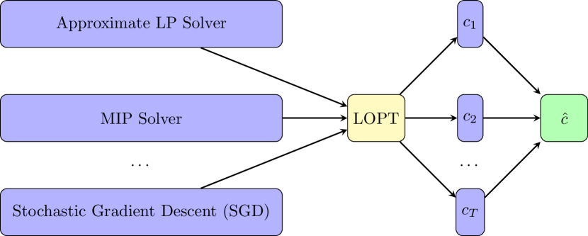
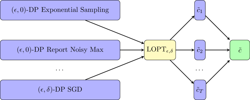
Figure 1: Approximate Linear Optimizer Oracles $\operatorname*{LOPT}$ and $\operatorname*{LOPT}_{\epsilon,\delta}$

As Figure 1 illustrates, $\operatorname*{LOPT}_{\epsilon,\delta}$ could be implemented via a number of approaches depending on the specification of the loss function $\ell$. For example, in the case where $\ell$ is convex and $\mathcal{C}_{P}$ lies in the $\ell_{2}$ unit ball, we can provide an implementation of a computationally efficient $\operatorname*{LOPT}_{\epsilon,\delta}$ based on the private stochastic gradient descent algorithm of Bassily et al. (2014) and use this oracle to, for example, solve weighted least squares regression (Sheffet, 2019). If $\ell$ is not convex, we could use more generic implementations of the exponential mechanism. Without privacy considerations, $\operatorname*{LOPT}$ can be implemented via the use of an approximate LP or MIP solver or via a vanilla stochastic gradient descent (Bubeck, 2015). The implementation of $\operatorname*{LOPT},\operatorname*{LOPT}_{\epsilon,\delta}$ will depend on the decision set $\mathcal{C}_{P}$ and its accompanying loss function $\ell$. In (Alabi et al., 2018), the existence of $\operatorname*{LOPT}$ is assumed and used to solve the CGOO problem non-privately. We shall also follow a similar route: assume the existence of $\operatorname*{LOPT}_{\epsilon,\delta}$ but, in addition, we will provide a generic implementation of the private oracle so that we may obtain utility guarantees.

In Section 8, we show applications of our work to two main suites of uses cases. The first is for optimizing convex performance measures of the confusion matrix (such as those derived from the $G$-mean and $H$-mean); the second is for satisfying statistical definitions of algorithmic fairness (such as equalized odds, demographic parity, and Gini index of inequality).

1.1 Summary of Results

We proceed to state and interpret informal versions of some of our main theorems and corollaries. Through the lens of information-theoretic reductions, we show the following:

1. Algorithms: Present two generic differentially private algorithms to solve this problem – an $(\epsilon,0)$ exponential sampling algorithm and an $(\epsilon,\delta)$ algorithm that uses an approximate linear optimizer to incrementally move toward the best decision.

2. Improvements on Sample Complexity Upper Bound: Compared to a previous method for ensuring differential privacy subject to a relaxed form of the equalized odds fairness constraint, the $(\epsilon,\delta)$-differentially private algorithm we present provides asymptotically better sample complexity guarantees, resulting in an exponential improvement in certain parameter regimes.

3. First Polynomial-Time Algorithms: Give the first polynomial-time algorithms to solve the problem with $(\epsilon,0)$ or $(\epsilon,\delta)$ differential privacy guarantees when defined on a convex decision set (for example, the $\ell_{P}$ unit ball) with convex constraints and losses.

4. Bounded Divergence Linear Optimizer Primitive: Introduce a class of bounded divergence linear optimizers and specialize to pure and approximate differential privacy. The technique of using bounded divergence linear optimizers to simultaneously achieve privacy/security (and/or other constraints) and utility might be applicable to other problems not considered in this paper.

5. Lower Bounds: Finally, we show an algorithm-agnostic information-theoretic lower bound on the excess risk (or equivalently, the sample complexity) of any solution to the problem of $(\epsilon,0)$ or $(\epsilon,\delta)$ differentially private constrained group-objective optimization.

Unlike in (Bassily et al., 2014), the sample complexity upper bounds for convex $\ell,f,g$ scale as $O(1/\alpha^{2})$ rather than $O(1/\alpha)$ because of the way we apply Lagrangian Duality. We essentially compose functions $f,g$ into $h=f+\max(0,g)\cdot O(\sqrt{K}/\alpha)$. As a result, to minimize $h$ to within $O(\alpha)$, we need to minimize $g$ to within $O(\alpha^{2}/\sqrt{K})$. As a consequence, our results are tight (with respect to the accuracy parameter $\alpha$) amongst all strategies that compose functions. In addition, when using differential privacy, the dependence on $P$ or $\operatorname*{VC}(\mathcal{C}_{P})$ is necessary because our methods sample from $P$-dimensional decision sets (while $K$ is the ambient dimension due to function composition).

Theorem (Informal) 1.5.

Suppose we are given any constrained group-objective optimization problem (Definition 1.2) where $f$ and $g$ are convex, Lipschitz functions and we wish to obtain a decision $\tilde{c}\in\mathcal{C}_{P}$ in a differentially private manner.

If $\ell$ is a convex function and $f,g$ are non-decreasing, then let $n_{0}=O(\frac{K\cdot P}{\epsilon\alpha^{2}})$. If not, let $n_{0}=\tilde{O}(\frac{K\cdot\operatorname*{VC}(\mathcal{C}_{P})}{\epsilon\alpha^{2}})$. Then there exists $n_{0}$ such that for all $n\geq n_{0}$ and privacy parameter $\epsilon>0$ there is an $\epsilon$-differentially private algorithm that, with probability at least 9/10, returns a decision $\tilde{c}\in\mathcal{C}_{P}$ that solves the $\textrm{CGOO}(\mathcal{C}_{P},n,K,f,g,\ell,D,\alpha)$ problem. The algorithm is guaranteed to be computationally efficient in the case where $\ell$ is convex and $f,g$ are non-decreasing.

Theorem 1.5 (more informal version of Theorem 5.2) shows that we can use the exponential mechanism to solve the $\textrm{CGOO}(\mathcal{C}_{P},n,K,f,g,\ell,D,\alpha)$ problem although an explicit mechanism to sample from the set $\mathcal{C}_{P}$ is not provided. This method provides a pure $\epsilon$-differentially private algorithm to solve the problem. The problem is easier and guaranteed to be computationally efficient when $\ell$ is convex and $f,g$ are non-decreasing because it results in an efficient construction of a $\operatorname*{LOPT}_{\epsilon,\delta}$ oracle with polynomial runtime in $P,K,n$. If not, we use the generic exponential mechanism and do not provide any computational efficiency guarantees.

Theorem (Informal) 1.6.

Suppose we are given any constrained group-objective optimization problem (Definition 1.2) where $f,g$ are convex, Lipschitz functions. Then for any $\alpha>0$, there exists an algorithm that after $T=O(\frac{K^{4}}{\alpha^{2}})$ calls to $\operatorname*{LOPT}$ will, with probability at least 9/10, return a decision $\hat{c}\in\mathcal{C}_{P}$ that solves the $\textrm{CGOO}(\mathcal{C}_{P},n,K,f,g,\ell,D,\alpha)$ problem.

Theorem (Informal) 1.7.

Suppose we are given any constrained group-objective optimization problem (Definition 1.2) where $f$ and $g$ are convex, Lipschitz functions and we wish to obtain a decision $\tilde{c}\in\mathcal{C}_{P}$ in a differentially private manner.

Then for any privacy parameters $\epsilon,\delta\in(0,1]$, there exists an $(\epsilon,\delta)$-differentially private linear optimization based algorithm for which there is a setting of $\epsilon^{\prime},\delta^{\prime}\in(0,1]$ such that after $T=O\left(\frac{K^{4}}{\alpha^{2}}\right)$ calls to $\operatorname*{LOPT}_{\epsilon^{\prime},\delta^{\prime}}$, with probability at least 9/10, the algorithm returns a decision $\tilde{c}\in\mathcal{C}_{P}$ that solves the $\textrm{CGOO}(\mathcal{C}_{P},n,K,f,g,\ell,D,\alpha)$ problem.

Theorem 1.6 (more informal version of Theorem 5.5) shows that for any accuracy parameter $\alpha>0$, we can, after $T=\operatorname*{poly}(K,1/\alpha)$ calls to a linear optimization oracle, solve the constrained group-objective optimization problem to within $\alpha$, with high probability, provided that $f,g$ are convex, Lipschitz functions. For this theorem, we require access to $\operatorname*{LOPT}$ in each iteration. We note that Alabi et al. (2018) also achieved this theorem but we reprove it here more generally (so it is more amenable to use in our later proofs involving the additional constraint of data privacy).

Theorem 1.7 (more informal version of Theorem 5.9), with privacy guarantees, still relies on calls to a linear optimization oracle albeit its private counterpart $\operatorname*{LOPT}_{\epsilon,\delta}$. One way to interpret Theorems 1.6 and 1.7 is that if the non-private oracle is replaced with the private oracle, we can still solve the $\textrm{CGOO}(\mathcal{C}_{P},n,K,f,g,\ell,D,\alpha)$ problem via the use of advanced composition (Dwork et al., 2010). What remains is to show the existence and construction of the oracle $\operatorname*{LOPT}_{\epsilon,\delta}$ and provide utility guarantees for certain constructions.

Theorem (Informal) 1.8.

For any privacy parameter $\epsilon>0$, there is an implementation of $\operatorname*{LOPT}_{\epsilon,0}$ based on the exponential mechanism.

For any $\tau>0,\theta\in(0,1]$, if $\ell$ is convex and $\mathcal{W}$ is restricted to non-negative vectors, set $n_{0}=\tilde{O}(\frac{\sqrt{K}}{\epsilon\tau}(P+\log\frac{1}{\theta}))$ and if not set $n_{0}=\tilde{O}(\frac{\sqrt{K}}{\epsilon\tau}(\operatorname*{VC}(\mathcal{C}_{P})+\log\frac{1}{\theta}))$. Then there exists $n_{0}$ such that for all $n\geq n_{0}$, we can solve the $\operatorname*{LOPT}^{\theta}_{\epsilon,0}(\mathcal{C}_{P},\ell,\text{{w}},D,\tau)$ problem.

Theorem 1.8 (more informal version of Theorem 5.10) shows a generic construction of the $\operatorname*{LOPT}^{\theta}_{\epsilon,0}$ oracle. Armed with this, we provide Corollary  1.9.

Corollary (Informal) 1.9.

Suppose we are given any constrained group-objective optimization problem (Definition 1.2) where $f$ and $g$ are convex, Lipschitz functions and we wish to obtain a decision $\tilde{c}\in\mathcal{C}_{P}$ in a differentially private manner.

For any privacy parameters $\epsilon,\delta\in(0,1]$, there exists an $(\epsilon,\delta)$-differentially private linear optimization based algorithm that solves the $\textrm{CGOO}(\mathcal{C}_{P},n,K,f,g,\ell,D,\alpha)$ problem. If $\ell$ is convex and $f,g$ are non-decreasing, set $n_{0}=\tilde{O}\left(\frac{K^{4}P}{\epsilon\alpha^{3}}\right)$. If not, set $n_{0}=\tilde{O}\left(\frac{K^{4}\cdot\operatorname*{VC}(\mathcal{C}_{P})}{\epsilon\alpha^{3}}\right)$. Then there exists $n_{0}$ such that for all $n\geq n_{0}$, with probability at least 9/10, the algorithm will return a decision $\tilde{c}\in\mathcal{C}_{P}$ that solves the $\textrm{CGOO}(\mathcal{C}_{P},n,K,f,g,\ell,D,\alpha)$ problem. The algorithm uses an $\operatorname*{LOPT}_{\epsilon,0}$ oracle implemented via the exponential mechanism.

In some ways, the statistical and computational complexity we obtain in Corollary 1.9 is worst-case since we implement the $\operatorname*{LOPT}_{\epsilon,0}$ oracle via the exponential mechanism. For specific problems (e.g., ordinary least squares on the $\ell_{2}$ ball), there are more computationally efficient implementations of the $\operatorname*{LOPT}_{\epsilon,\delta}$ oracle as we shall see in Section 1.3. We show asymptotic convergence guarantees so that the excess risk goes to 0 as $n\rightarrow\infty$. For ease of exposition, the sample complexity guarantees of Theorem 1.7, 1.8, and 1.9 are in terms of $\tilde{O}(\cdot)$ which hides polylogarithmic factors (including the polylogarithmic dependence on $\frac{1}{\delta}$). We ignore these polylogarithmic factors to obtain cleaner statements.

Theorem (Informal) 1.10.

Suppose we are given a constrained group-objective optimization problem (Definition 1.2) where $f$ and $g$ are convex functions. Let $\epsilon>0$. Then for every $\epsilon$-differentially private algorithm, there exists a dataset $D=\{\text{{x}}_{1},\ldots,\text{{x}}_{n}\}$ drawn from the $\ell_{2}$ unit ball such that, with probability at least 1/2, in order to solve the problem $\textrm{CGOO}(\mathcal{C}_{P},n,K,f,g,\ell,D,\alpha)$ we need sample size $n\geq\Omega\left(\frac{K}{\epsilon\alpha}\right)$.

Theorem (Informal) 1.11.

Suppose we are given a constrained group-objective optimization problem (Definition 1.2) where $f$ and $g$ are convex functions. Let $\epsilon>0,\delta=o(\frac{1}{n})$. Then for every $(\epsilon,\delta)$-differentially private algorithm, there exists a dataset $D=\{\text{{x}}_{1},\ldots,\text{{x}}_{n}\}$ drawn from the $\ell_{2}$ unit ball such that, with probability at least 1/3, in order to solve the problem $\textrm{CGOO}(\mathcal{C}_{P},n,K,f,g,\ell,D,\alpha)$ we need sample size $n\geq\Omega\left(\frac{\sqrt{K}}{\epsilon\alpha}\right)$.

Theorems 1.10 and 1.11 (more informal versions of Theorems 6.1 and 6.2) show lower bounds on the sample complexity for solving the constrained group-objective optimization problem in a differentially private manner. The lower bounds for achieving (pure) $\epsilon$ and (approximate) $(\epsilon,\delta)$-differential privacy to solve the $\textrm{CGOO}(\mathcal{C}_{P},n,K,f,g,\ell,D,\alpha)$ problem differs from the upper bounds (from Theorems 1.5 and 1.7). Note that this gap is a direct result of the way we minimize $f$ subject to the constraint of $g$ by jointly minimizing a composition of these functions. As a consequence, our results are optimal amongst all such strategies that jointly minimize a composition of these functions.

We note that (Jagielski et al., 2018) considered the problem of differentially private fair learning in which they present a reductions approach to fair learning but the oracle-based algorithms they provide are specific modifications of those provided by Agarwal et al. (2018). The algorithm is an exponentiated gradient algorithm for fair classification that uses a cost-sensitive classification oracle solver in each iteration, which is only applied to the equalized odds definition. We show an approach that applies to more than one definition. Moreover, the algorithms in our paper results in asymptotically better sample complexity guarantees than previous work although under different underlying oracle assumptions and for a smoothed version of the equalized odds definition.

We hope that the generality of our approaches and techniques here will lead to applications in myriad domains.

1.2 Techniques

We introduce a class of bounded divergence linear optimizers (see Section 7) to simultaneously achieve strong privacy guarantees and solve constrained group-objective optimization problems (Definition 1.2). These linear optimizers can be used to solve general multi-objective problems with one or more divergence constraints. For simplicity and clarity of exposition, we specialize this linear optimizer to $(\epsilon,0)$ and $(\epsilon,\delta)$-differential privacy.

Based on the exponential mechanism, we provide an $(\epsilon,0)$-differentially private algorithm to solve the CGOO problem. In the case where $\ell$ is convex, we use the computationally efficient sampling technique of Bassily et al. (2014) to sample from $\mathcal{C}_{P}$. Our CGOO algorithms rely on the simple observation that if we are given two functions $f,g:[0,1]^{K}\rightarrow{\mathbb{R}}$ and aim to minimize the function $f$ subject to the constraint $g$ we could minimize them jointly via a “new” function. Specifically, we define the function $h:[0,1]^{K}\rightarrow{\mathbb{R}}$ where $h(\text{{x}})=f(\text{{x}})+G\cdot\max(0,g(\text{{x}}))$ for all $\text{{x}}\in[0,1]^{K}$ for some setting of $G>0$. Then we could optimize $h$ with privacy in mind. The $(\epsilon,\delta)$-differentially private algorithm, in each iteration, relies on calls to the private oracle $\operatorname*{LOPT}_{\epsilon,\delta}$. And to optimize both $f$ and $g$ to within $\alpha$ we can set $G=O(\frac{\sqrt{K}}{\alpha})$ (for large enough sample size $n$). Note that this differentially private algorithm is a first-order iterative optimization algorithm that relies on access to the gradient oracles $\nabla f,\nabla g$. Optimization with respect to these gradient oracles is done in a private manner while weighting $\nabla g$ by a multiplicative factor of $G$. The strategy of differentially private optimization of a function subject to one or more constraints can be applied to other situations. The weighting of gradients non-privately to solve the $\textrm{CGOO}(\mathcal{C}_{P},n,K,f,g,\ell,D,\alpha)$ problem was done by Alabi et al. (2018) but without privacy considerations. The technique of using the private oracle $\operatorname*{LOPT}_{\epsilon,\delta}$ (or an alternative from the class of bounded divergence linear optimizers) to solve an overall convex (or non-convex) optimization problem, with or without other constraints, might be applicable to other scenarios.

It is known that differentially private iterative algorithms use the crucial property of (advanced) composition of differential privacy (Dwork et al., 2010; Dwork and Roth, 2014) which come in a variety of forms. The iterative algorithms we provide exploit this property. The lower bounds we provide for empirical risk minimization are modified versions of the ones provided by Bassily et al. (2014).

1.3 Applications

In computer science, showing that one problem can be reduced to another is a staple of proofs, to obtain lower or upper bounds on complexity measures. Karp (1972), famously, showed that there is a many-to-one reduction from the Boolean Satisfiability problem to 21 graph-theoretical and combinatorial problems. Karp showed that, as a consequence, these 21 problems are NP-complete.

This approach of using reductions can also be applied to problems that are not necessarily combinatorial in nature. We, essentially, reduce a few problems to solving bounded-divergence linear subproblems (see Section 7).

Method	Desired Guarantees
$\ell_{0}$	Sparsity, Basis Selection
$\ell_{1}$	Robustness to Outliers, Transfer of Compressed Sensing Techniques
$\ell_{2}$	Standard (and Faster) Convergence Rates, Allows (Provable) use of SGD Based Methods

Table 1: Comparing properties of $\ell_{0},\ell_{1},\ell_{2}$ minimization (Wipf and Rao, 2004; Donoho, 2006)

After using Lagrangian duality to create objectives that satisfy one or more sub-criteria, we can rely on calls to standard optimizers. The choice of the underlying optimizer depends on the desired properties we want to satisfy. See Table 1 for examples. The use of robust differentially private estimators (e.g., $\ell_{1}$ objectives) could provide better utility (Dwork and Lei, 2009).

In Section 8, we expand on the breadth of our applications from optimizing convex measures of the confusion matrix to satisfying certain definitions from the algorithmic fairness literature. The linear optimization based algorithm we provide can only be applied to convex, Lipschitz functions $f,g$. In the appendix, we provide a Frank-Wolfe based algorithm that also requires Lipschitz gradients. However, we note that even if $f,g$ are not convex or smooth there exist surrogate convex functions and standard smoothing techniques that can be applied (e.g., see Moreau-Yosida regularization (Nesterov, 2005) and correspondences between $f$-divergences and surrogate loss functions (Bartlett et al., 2006; Nguyen et al., 2005, 2009)). First, we show how to apply our work to the problem of weighted least squares regression. Then, we show how to satisfy a relaxed form of the Equalized Odds fairness definition while returning accurate classifiers on training data. Finally, we apply our results to the problem of hypothesis testing.

1.3.1 Case Study: Reduction to Ordinary Least Squares with Subgroup Weights

We have stated approaches to solving the $\textrm{CGOO}(\mathcal{C}_{P},n,K,f,g,\ell,D,\alpha)$ problem using a generic construction of $\operatorname*{LOPT}_{\epsilon,\delta}$ oracles via the exponential mechanism which is not guaranteed to be computationally efficient. Now we proceed to show that for the specific problem of ordinary least squares (which admits a convex loss), we get an efficient $\operatorname*{LOPT}_{\epsilon,\delta}$.

Let $B^{P}_{2}$ represent the unit ball in $P$ dimensions i.e., $B^{P}_{2}=\{\text{{x}}\in{\mathbb{R}}^{P}:\mathopen{\|}\text{{x}}\mathclose{\|}_{2}=1\}$. Suppose we are given $n>1$ input points $\text{{x}}_{1},\ldots,\text{{x}}_{n}$ from $B^{P}_{2}$ each belonging to one of $[K]$ groups encoded through a function $d:B^{P}_{2}\rightarrow[K]$ (i.e., private function known to the data curator). Each data point $\text{{x}}_{i}$ has a corresponding output point $y_{i}\in[0,1]$.

Given a weight vector $\text{{w}}\in[0,1]^{K}$, the goal is to output a $c\in B^{P}_{2}$ such that the empirical average squared loss

$$\frac{1}{n}\sum_{k\in[K]}\sum_{i=1}^{n}w_{k}\cdot\ell_{k}(c,\text{{x}}_{i},y_{i})=\frac{1}{n}\sum_{k\in[K]}\sum_{i=1}^{n}w_{k}\cdot\mathds{1}[d(\text{{x}}_{i})=k]\cdot(\langle c,\text{{x}}_{i}\rangle-y_{i})^{2}$$

is minimized. To proceed, a naive method is to translate each $\text{{x}}_{i}\in B^{P}_{2}$ into $\bar{\text{{x}}}_{i}\in B^{PK}_{2}$ where $\text{{x}}_{i}$ will occupy coordinates $(k-1)P+1,\ldots,k\cdot P$ of $\bar{\text{{x}}}_{i}$ if $\text{{x}}_{i}$ belongs to group $k\in[K]$. The remaining coordinates will be set to 0. We now routinely apply the private stochastic gradient algorithm of  Bassily et al. (2014) to solve the $\operatorname*{LOPT}_{\epsilon,\delta}$ problem in time polynomial in $K,P$ and thus solve the $\textrm{CGOO}(\mathcal{C}_{P},n,K,f,g,\ell,D,\alpha)$ problem in time polynomial in $K,P$. But note that this results in a regression coefficient vector in $B^{PK}_{2}$ instead of $B^{P}_{2}$. A similar idea can be used to obtain coefficient vectors in $B^{P}_{2}$ instead.

Note that since the loss function $\ell_{k}(c,\text{{x}}_{i},y_{i})=\mathds{1}[d(\text{{x}}_{i})=k]\cdot(\langle c,\text{{x}}_{i}\rangle-y_{i})^{2}$ has Lipschitz constant at most 2, we get the following corollary by, for example, using the $(\epsilon,\delta)$-differentially private stochastic gradient descent algorithm in  (Bassily et al., 2014) to implement $\operatorname*{LOPT}_{\epsilon,\delta}$.

Corollary (Informal) 1.12.

There exists a polynomial-time $(\epsilon,\delta)$-differentially private algorithm that, with probability at least 9/10, returns a decision $\tilde{c}\in\mathcal{C}_{p}$ that solves the $\textrm{CGOO}(\mathcal{C}_{P},n,K,f,g,\ell,D,\alpha)$ problem when applied to solve ordinary least squares.

We have discussed how to obtain efficient oracles for $\operatorname*{LOPT},\operatorname*{LOPT}_{\epsilon,\delta}$. But how do different implementations of $\operatorname*{LOPT},\operatorname*{LOPT}_{\epsilon,\delta}$ perform (relative to one another) for the weighted least squares regression problem? And how can we use these $\operatorname*{LOPT},\operatorname*{LOPT}_{\epsilon,\delta}$ oracles to solve the CGOO problem?  Agarwal et al. (2019) study fair regression via reduction-based algorithms, an approach that can be instantiated in the CGOO framework. The weighted linear regression problem can be solved differentially privately as shown in (Sheffet, 2019). We defer the study of this problem in detail (with specific applications to regression) to future work.

1.3.2 Case Study: Satisfying Equalized Odds

We proceed to state an informal corollary that illustrates how to use our theorems to satisfy certain definitions from the algorithmic fairness literature. The corollary serves to compare the method in this paper to that of  Jagielski et al. (2018) in satisfying $\alpha$-equalized odds (see Definition 1.13) which is the only fairness definition they consider when satisfying both privacy and fairness. In contrast, the algorithms in this paper can be applied to more than one kind of fairness definition (although under different oracle assumptions). Also, our linear optimization based algorithm requires not just convexity of $f,g$ but also that $f,g$ are Lipschitz so we define a smoothed version of the Equalized Odds definition.

Definition 1.13 ($\alpha$-Equalized Odds (Jagielski et al., 2018)).

Let $X,A,Y$ be random variables representing the non-sensitive features, the sensitive attribute, and the label assigned to an individual, respectively.

Given a dataset of examples $D=\{(\text{{x}}_{i},a_{i},y_{i})\}_{i=1}^{n}\in(\mathcal{X},\mathcal{A},\{0,1\})^{n}$ of size $n$, we say a classifier $c\in\mathcal{C}_{P}$ satisfies $\alpha$-Equalized Odds if

$$\max_{a,a^{\prime}\in\mathcal{A}}\{\max(|\hat{FP}_{a}-\hat{FP}_{a^{\prime}}|,|\hat{TP}_{a}-\hat{TP}_{a^{\prime}}|)\}\leq\alpha$$ (1)

where $\hat{FP}_{a},\hat{TP}_{a}$ are empirical estimates of $FP_{a}(c)=\mathbb{P}_{(\text{{x}},a,y)}[c(\text{{x}})=1|A=a,y=0]$, $TP_{a}(c)=\mathbb{P}_{(\text{{x}},a,y)}[c(\text{{x}})=1|A=a,y=1]$ respectively on dataset $D$.

We say a classifier satisfies $\alpha$-Smoothed Equalized Odds if the smoothed version of Equation 1 is satisfied (i.e., when the maximum and absolute functions in Equation 1 are replaced with smoothed versions or using the Moreau-Yosida regularization technique).

For concreteness, we provide a specific smoothed version of $\alpha$-equalized odds in Definition 1.14.

Definition 1.14 ($(\alpha,\eta)$-Smoothed Equalized Odds).

Let $X,A,Y$ be random variables representing the non-sensitive features, the sensitive attribute, and the label assigned to an individual, respectively.

Given a dataset of examples $D=\{(\text{{x}}_{i},a_{i},y_{i})\}_{i=1}^{n}\in(\mathcal{X},\mathcal{A},\{0,1\})^{n}$ of size $n$, we say a classifier $c\in\mathcal{C}_{P}$ satisfies $(\alpha,\eta)$ Equalized Odds if the constraint function

$$g(\hat{FP},\hat{FN},\hat{TP})=\operatorname*{smax}^{\eta}_{a,a^{\prime}\in\mathcal{A}}\{\max(|\hat{FP}_{a}-\hat{FP}_{a^{\prime}}|,|\hat{TP}_{a}-\hat{TP}_{a^{\prime}}|)\}-\alpha$$ (2)

is less than or equal to 0. $(\hat{FP},\hat{FN},\hat{TP})$ corresponds to the $3|\mathcal{A}|$ empirical estimates of the false positives, false negatives, and true positives for the $|\mathcal{A}|$ groups. $(\hat{FP},\hat{TP})$ are used to enforce the equalized odds constraint while $(\hat{FP},\hat{FN})$ are used to compute the error of the classifier. We use the smooth maximum function $\operatorname*{smax}^{\eta}(y_{1},\ldots,y_{n})=\frac{\sum_{i=1}^{n}y_{i}e^{\eta y_{i}}}{\sum_{i=1}^{n}e^{\eta y_{i}}}$ (Lange et al., 2014) as a replacement for the non-smooth maximum function. As $\eta\rightarrow\infty$, $\operatorname*{smax}^{\eta}\rightarrow\max$.

Note that the solutions that satisfy Definition 1.13 might differ from the ones that satisfy Definition 1.14 because of the cost of smoothing parameterized by $\eta$. Also, the gradient of $\operatorname*{smax}^{\eta}$ is given by $\nabla_{y_{i}}\operatorname*{smax}^{\eta}(y_{1},\ldots,y_{n})=\frac{e^{\eta y_{i}}}{\sum_{j=1}^{n}e^{\eta y_{j}}}[1+\eta(y_{i}-\operatorname*{smax}^{\eta}(y_{1},\ldots,y_{n}))]$.

Corollary (Informal) 1.15.

For any privacy parameters $\epsilon,\delta\in(0,1]$, suppose we have a dataset of examples $D=\{(\text{{x}}_{i},a_{i},y_{i})\}_{i=1}^{n}$ of size $n$ where $\text{{x}}_{i}\in\mathcal{X},y_{i}\in\{0,1\}$, $a_{i}\in\mathcal{A}$, for all $i\in[n]$. Assume that there exists at least one decision in $\mathcal{C}_{P}$ (with finite VC dimension of at most $\operatorname*{VC}(\mathcal{C}_{P})$) that satisfies $(\alpha,\eta)$-Smoothed Equalized Odds (by Definition 1.14) for some $\eta>0$.

Then there exists $n_{0}=\tilde{O}\left(\frac{|\mathcal{A}|^{4}\cdot\operatorname*{VC}(\mathcal{C}_{P})}{\epsilon\alpha^{3}}\right)$ such that for all $n\geq n_{0}$, given access to a $\operatorname*{LOPT}_{\epsilon,\delta}$ oracle, we can, with probability at least $9/10$, obtain a decision $\tilde{c}\in\mathcal{C}_{P}$ satisfying $(\alpha,\eta)$-smoothed equalized odds and that is within $\alpha$ away from the most accurate classifier.

We provide the proof for Corollary 1.15 as Corollary 8.9 in Section 8. Corollary 1.15 uses Theorem 5.9 as the base theorem. In comparison, in the regime where, in their formulation, $\min_{a,y}\{\hat{q}_{ay}\}\leq\alpha^{(1+r)/2}$ for any $r>0$ (see Section C in the Appendix for more details), their methods can solve the $\textrm{CGOO}(\mathcal{C}_{P},n,K,f,g,\ell,D,\alpha)$ problem using sample complexity $\tilde{O}\left(\frac{|\mathcal{A}|^{3}\cdot\operatorname*{VC}(\mathcal{C}_{P})}{\epsilon\alpha^{3+r}}\right)$. In Section C, we state their main theorem (Theorem C.1) and a corollary (Corollary  C.2) showing the sample complexity required for their algorithm to solve the $\textrm{CGOO}(\mathcal{C}_{P},n,K,f,g,\ell,D,\alpha)$ problem when applied to the Equalized Odds fairness definition. On the other hand, Corollary 1.15 results in sample size $\tilde{O}\left(\frac{|\mathcal{A}|^{4}\cdot\operatorname*{VC}(\mathcal{C}_{P})}{\epsilon\alpha^{3}}\right)$. As a result, by Corollary 1.15, the linear optimization based algorithm for Theorem 5.9 performs better for all $r>0$ and $|\mathcal{A}|<1/\alpha^{r}$ (in terms of asymptotic sample complexity for the accuracy parameter $\alpha>0$) than the DP-oracle-learner (which uses a private version of a cost-sensitive classification oracle $\operatorname*{CSC}(\mathcal{C}_{P})$ in each iteration of their algorithm) of Jagielski et al. (2018). Comparing the results of Jagielski et al. (2018) to Corollary 1.15, we see that our results hold under different oracle assumptions and for a smoothed version of the equalized odds constraint. As a result, the comparison is not as direct as we would like.

1.3.3 Case Study: Privately Selecting Powerful Statistical Tests

Essentially, any problem that can be simulated via the use of a confusion matrix (i.e., empirical estimates of Type I, II error) can be solved using our framework.

Our results can also be applied to hypothesis testing to, for example, select high-power test statistics. A hypothesis is simple if it completely specifies the data distribution. The hypothesis $H_{i}:\theta\in\Omega_{i}$ is simple when $|\Omega_{i}|=1$. Let $Y$ be the observed data. For such simple hypothesis, let $p_{0},p_{1}$ denote densities of $Y$ under $H_{0}$ (the null hypothesis) and $H_{1}$ (the alternative) respectively. When both $H_{0},H_{1}$ are simple then the Neyman-Pearson lemma completely characterizes all tests on the competing hypothesis via the likelihood ratio $L(y)=p_{1}(y)/p_{0}(y)$ (Keener, 2010). For any $y$, let $p_{0}(y),p_{1}(y)$ denote the density of $y$ under $H_{0}$ and $H_{1}$ respectively. Anagolues of the Neyman-Pearson lemma have been studied in the differential privacy literature (Kairouz et al., 2017; Canonne et al., 2019).

The power function for a simple test function $\phi$ (that returns the probability of rejecting the null hypothesis) has two possible values:

$$\alpha=\gamma_{0}=\mathbb{E}_{0}\phi=\int\phi(y)p_{0}(y)dy,\quad\gamma_{1}=\mathbb{E}_{1}\phi=\int\phi(y)p_{1}(y)dy,$$

where the level is $\alpha$ should be as close to zero as possible and $\gamma_{1}$ should be close to one. The goal would be to maximize $\gamma_{1}$ among all tests $\phi$ with $\alpha=\mathbb{E}_{0}\phi$. This is a constrained maximization problem, for which our work shows the existence of oracle-efficient differentially private (empirical risk) solvers for a fixed dataset $Y$. See the informal Corollary 1.17, which follows from the formal Corollary 5.11 statement.

Proposition 1.16 (Neyman-Pearson Lemma (Neyman et al., 1933)).

Given any level $\alpha=\mathbb{E}_{0}\phi\in[0,1]$, there exists a likelihood ratio test $\phi_{\alpha}$ with level $\alpha$ and any likelihood ratio test with level $\alpha$ maximizes $\mathbb{E}_{1}\phi$ among all tests with level at most $\alpha$.

Corollary (Informal) 1.17.

There exists an oracle-efficient $(\epsilon,\delta)$-differentially private algorithm that, with probability at least 9/10, returns a test statistic with target significance level $\alpha\in(0,1]$ and is $\alpha$ away from the most powerful test statistic.

We defer the explicit construction of such algorithms (for privately selecting high-power test statistics) to future work.

2 Related Work

Below we briefly specify a few other works related to the material presented in this paper.

Adversarial Prediction: Adversarial prediction (via Lagrangian duality, for example) for multi-objective optimization is the main workhorse of most algorithmic fairness frameworks (Freund and Schapire, 1997; Wang et al., 2015). Multi-objective adversarial prediction builds off of work of mathematicians David Blackwell (Blackwell’s Approachability Theorem  (Blackwell, 1956)) and James Hannan (Hannan, 1957). See (Cesa-Bianchi and Lugosi, 2006) for a survey on learning and games.

Alghamdi et al. (2020) define a model projection framework which can be viewed via the lens of Lagrangian duality but do not analyze the computational efficiency of their solutions. We aim to delineate the computational efficiency of such information-theoretic problems.

Reductions Approach to Fair Classification and Regression: Agarwal et al. (2018) explore the problem of using black-box optimizers to minimize group-fair convex objectives subject to constraint functions. Alabi et al. (2018) extend this work to handle any Lipschitz-continuous group objective of losses given oracle access to an approximate linear optimizer in time polynomial in the inverse of the accuracy parameter. Furthermore, they extend their results to learning using a polynomial number of examples and access to an agnostic learner. Our definition of the constrained group-objective optimization problem is inspired by the work and results of Alabi et al. (2018). Additionally, Narasimhan et al. (2015); Narasimhan (2018); Hiranandani et al. (2019) explore optimizing convex objectives of the confusion matrix (such as those derived from $G$-mean, $H$-mean typically used for class-imbalanced problems) and fractional-convex functions of the confusion matrix (such as $F_{1}$ measure used in text retrieval).

In this paper, we consider some of the use cases explored by previous works but also add on the additional constraint of data privacy, an important constraint given that fairness is often imposed with respect to the sensitive attributes of data subjects.

Private Empirical Risk Minimization: Differentially private empirical risk minimization in the convex setting has been considered in a variety of settings (Chaudhuri et al., 2011; Kifer et al., 2012; Bassily et al., 2014; Talwar et al., 2014, 2015; Steinke and Ullman, 2015; Wang et al., 2018; Iyengar et al., 2019) with algorithm-specific upper and algorithm-agnostic lower bounds provided in some cases. We largely build upon these works.

Private Fair Learning: Jagielski et al. (2018) initiate the study of differentially private fair learning but only consider the equalized odds definition in the reductions approach to fair learning. Ekstrand et al. (2018) discuss an agenda for subproblems that should be considered when trying to achieve data privacy for fair learning. Last, Kilbertus et al. (2018) study how to learn models that are fair by encrypting sensitive attributes and using secure multiparty computation.

3 Preliminaries and Notation

Here we introduce preliminaries and notation that might be useful to parse through later sections.

3.1 Differential Privacy

For the definitions below, for any two datasets $D,D^{\prime}\in\mathcal{Z}^{n}$, we use $D\sim D^{\prime}$ to mean that $D$ and $D^{\prime}$ are neighboring datasets that differ in exactly one row.

Definition 3.1 ((Pure) $\epsilon$-Differential Privacy (Dwork et al., 2006)).

For any $\epsilon\geq 0$, we say that a (randomized) mechanism $\mathcal{M}:\mathcal{Z}^{n}\rightarrow\mathcal{R}$ is $\epsilon$-differentially private if for every two neighboring datasets $D\sim D^{\prime}\in\mathcal{Z}^{n}$, we have that

$$\forall T\subseteq\mathcal{R},\mathbb{P}[\mathcal{M}(D)\in T]\leq e^{\epsilon}\cdot\mathbb{P}[\mathcal{M}(D^{\prime})\in T].$$

We usually take $\epsilon$ to be small but not cryptographically small. For example, typically we set $\epsilon\in[0.1,1]$. The smaller $\epsilon$ is, the more privacy is guaranteed.

Definition 3.2 ((Approximate) $(\epsilon,\delta)$-Differential Privacy).

For any $\epsilon\geq 0,\delta\in[0,1]$, we say that a (randomized) mechanism $\mathcal{M}:\mathcal{Z}^{n}\rightarrow\mathcal{R}$ is $(\epsilon,\delta)$-differentially private if for every two neighboring datasets $D\sim D^{\prime}\in\mathcal{Z}^{n}$, we have that

$$\forall T\subseteq\mathcal{R},\mathbb{P}[\mathcal{M}(D)\in T]\leq e^{\epsilon}\cdot\mathbb{P}[\mathcal{M}(D^{\prime})\in T]+\delta.$$

We insist that $\delta$ be cryptographically negligible i.e., $\delta\leq n^{-\omega(1)}$. The value $\delta$ can be interpreted as an upper-bound on the probability of a catastrophic event (such as publishing the entire dataset)(Vadhan, 2017). $(\epsilon,\delta)$-differential privacy can also be interpreted as “(pure) $\epsilon$-differential privacy with probability at least $1-\delta$.” The smaller $\epsilon$ and $\delta$ are, the more privacy is guaranteed.

Definition 3.3 ($\ell_{1}$-sensitivity of a function).

The $\ell_{1}$ sensitivity of a function $f:\mathcal{Z}^{n}\rightarrow{\mathbb{R}}^{K}$ is

$$\Delta_{1}(f)=\max_{D,D^{\prime}\in\mathcal{Z}^{n}:D\sim D^{\prime}}\mathopen{\|}f(D)-f(D^{\prime})\mathclose{\|}_{1},$$

where $D\sim D^{\prime}\in\mathcal{Z}^{n}$ are neighboring datasets.

Definition 3.4 ($\ell_{2}$-sensitivity of a function).

The $\ell_{2}$ sensitivity of a function $f:\mathcal{Z}^{n}\rightarrow{\mathbb{R}}^{K}$ is

$$\Delta_{2}(f)=\max_{D,D^{\prime}\in\mathcal{Z}^{n}:D\sim D^{\prime}}\mathopen{\|}f(D)-f(D^{\prime})\mathclose{\|}_{2},$$

where $D\sim D^{\prime}\in\mathcal{Z}^{n}$ are neighboring datasets.

Theorem 3.5 (Exponential Mechanism (McSherry and Talwar, 2007)).

For any privacy parameter $\epsilon>0$ and any given loss function $h:\mathcal{C}_{P}\times\mathcal{Z}^{n}\rightarrow{\mathbb{R}}$ and database $D\in\mathcal{Z}^{n}$, the Exponential mechanism outputs $c\in\mathcal{C}_{P}$ with probability proportional to $\exp(\frac{-\epsilon\cdot h(c,D)}{2\Delta h})$ where

$$\Delta h=\max_{c\in\mathcal{C}_{P}}\max_{D,D^{\prime}\in\mathcal{Z}^{n}:D\sim D^{\prime}}|h(c,D)-h(c,D^{\prime})|$$

is the sensitivity of the loss function $h$.

Theorem 3.6 (Privacy-Utility Tradeoffs of Exponential Mechanism (McSherry and Talwar, 2007)).

For any database $D\in\mathcal{Z}^{n}$, let $c^{*}=\operatorname*{argmin}_{c\in\mathcal{C}_{P}}h(c,D)$ and $\tilde{c}_{\epsilon}\in\mathcal{C}_{P}$ be the output of the Exponential Mechanism satisfying $\epsilon$-differential privacy. Then with probability at least $1-\rho$,

$$|h(\tilde{c}_{\epsilon},D)-h(c^{*},D)|\leq\log\left(\frac{|\mathcal{C}_{P}|}{\rho}\right)\left(\frac{2\Delta h}{\epsilon}\right).$$

Lemma 3.7 (Post-Processing (Dwork et al., 2006)).

Let $\mathcal{M}:\mathcal{Z}^{n}\rightarrow\mathcal{R}$ be an $(\epsilon,\delta)$-differentially private algorithm and $f:\mathcal{R}\rightarrow\mathcal{T}$ be any (randomized) function. Then $f\circ\mathcal{M}:\mathcal{Z}^{n}\rightarrow\mathcal{T}$ is an $(\epsilon,\delta)$-differentially private algorithm.

The exponential mechanism will be used as the main building block for our differentially private algorithms for constrained group-objective optimization. The Laplace and Gaussian mechanisms (Dwork and Roth, 2014; Dwork et al., 2006) are often used when the goal is to output estimates to a query (e.g., the mean, sum, or median) while the Exponential mechanism is used when the goal is to output an object (e.g., a regression coefficient vector or classifier) with minimum loss (or maximum utility).

3.2 Convexity, Smoothness, and Optimization Oracles

Definition 3.8 (Convex Set).

A set $\mathcal{V}\subset{\mathbb{R}}^{m}$ is a convex set if it contains all of its line segments. That is, $\mathcal{V}$ is convex iff

$$\forall\,\,(\text{{x}},\mathbf{y},\gamma)\in\mathcal{V}\times\mathcal{V}\times[0,1],\,\,(1-\gamma)\text{{x}}+\gamma\mathbf{y}\in\mathcal{V}.$$

Definition 3.9 (Convex Function).

A function $f:\mathcal{V}\rightarrow{\mathbb{R}}$ is a convex function if it always lies below its chords. That is, $f$ is convex iff

$$\forall\,\,(\text{{x}},\mathbf{y},\gamma)\in\mathcal{V}\times\mathcal{V}\times[0,1],\,\,f((1-\gamma)\text{{x}}+\gamma\mathbf{y})\leq(1-\gamma)f(\text{{x}})+\gamma f(\mathbf{y}).$$

Definition 3.10 (Subgradients).

Let $\mathcal{V}\subset{\mathbb{R}}^{m}$ and define a function $f:\mathcal{V}\rightarrow{\mathbb{R}}$. Then we say that $\bm{g}\in{\mathbb{R}}^{m}$ is a subgradient of $f$ at $\text{{x}}\in\mathcal{V}$ if for any $\mathbf{y}\in\mathcal{V}$ we have that

$$f(\text{{x}})-f(\mathbf{y})\leq\bm{g}^{T}(\text{{x}}-\mathbf{y}).$$

We denote $\partial f(x)$ as the set of subgradients of the function $f$ at $x\in\mathcal{V}$.

Definition 3.11 (Lipschitz Function).

Let $\mathcal{V}\subset{\mathbb{R}}^{m}$. A function $f:\mathcal{V}\rightarrow{\mathbb{R}}$ is $L$-Lipschitz on $\mathcal{V}$ if for all $\text{{x}},\mathbf{y}\in\mathcal{V}$, we have

$$|f(\text{{x}})-f(\mathbf{y})|\leq L\mathopen{\|}\text{{x}}-\mathbf{y}\mathclose{\|}.$$

Definition 3.12 ($\beta$-Smooth Function).

Let $\mathcal{V}\subset{\mathbb{R}}^{m}$. A function $f:\mathcal{V}\rightarrow{\mathbb{R}}$ is $\beta$-smooth if the gradient $\nabla f$ is $\beta$-Lipschitz. That is, for all $\text{{x}},\mathbf{y}\in\mathcal{V}$,

$$\mathopen{\|}\nabla f(\text{{x}})-\nabla f(\mathbf{y})\mathclose{\|}\leq\beta\cdot\mathopen{\|}\text{{x}}-\mathbf{y}\mathclose{\|}.$$

Note that if $f$ is twice-differentiable then $f$ being $\beta$-smooth is equivalent to the eigenvalues of its Hessians being smaller than $\beta$.

For our iterative algorithms, we assume access to a linear optimizer oracle that can solve subproblems of the form

$$y_{t}\in\operatorname*{argmin}_{\mathbf{y}\in\mathcal{V}}\text{{w}}^{T}\mathbf{y}$$

whether exactly or approximately for any $\text{{w}}\in\mathcal{V}\subset{\mathbb{R}}^{m}$. We previously defined non-private and private approximate linear optimizer oracles $\operatorname*{LOPT},\operatorname*{LOPT}_{\epsilon,\delta}$. We will assume the existence of $\operatorname*{LOPT}$ and provide a generic construction of its private counterpart.

The overall convex optimization problem will be converted into a series of linear subproblems. A key property of the use of linear optimizers in the (vanilla) Frank-Wolfe algorithm is that the projection step of projected gradient descent algorithms is replaced with a linear optimization step over the set $\mathcal{V}$. In some cases, solving linear optimization subproblems will be simpler and more computationally efficient to solve than projections into some feasible set.

4 Constrained Group-Objective Optimization via Weighting

In this section, we present a key lemma and corollary that will be crucial to the algorithms we will present in this paper. The iterative linear optimization based algorithms will solve the constrained group-objective optimization problem (Definition 1.2) in the setting where $f,g$ are convex, Lipschitz functions.

For the iterative algorithms we will present, we assume that $\mathcal{C}_{P}$ is closed under randomization. That is, for every $c_{1},\ldots,c_{T}\in\mathcal{C}_{P}$, if $c\in\Delta(\{c_{i}\}_{i=1}^{T})$ then $c\in\mathcal{C}_{P}$. For any $i\in[T]$, $c$ will predict $c_{i}(x)$ with probability $w_{i}$ where $\sum_{i=1}^{T}w_{i}=1$. We also assume that we can return randomized decisions defined over $\Delta(\mathcal{C}_{P})$.

Having settled on a reductionist optimization problem (Definition 1.2), the goal will be to obtain a decision $\hat{c}\in\mathcal{C}_{P}$ for which

$$\mathbb{E}[f(\ell(\hat{c},D))]\leq f(\ell(c^{*},D))+\alpha,\, \mathbb{E}[g(\ell(\hat{c},D))]\leq\alpha$$

OR

$$\text{ w.p. }\geq 1-\rho,\,\rho\in(0,1),\quad f(\ell(\hat{c},D))\leq f(\ell(c^{*},D))+\alpha,\, g(\ell(\hat{c},D))\leq\alpha$$ (3)

where $f,g:[0,1]^{K}\rightarrow{\mathbb{R}}$ are functions for which $c^{*}\in\operatorname*{argmin}_{c\in\mathcal{C}_{P}:g(\ell(c,D))\leq 0}f(\ell(c,D))+\alpha$ is the best decision (according to $f(\cdot)$) that satisfies the constraint function $g(\cdot)$ and $D$ is a fixed dataset of size $n$. The expectation or the high probability bound is over the random coins of the algorithm that chooses $\hat{c}$.

To reach the guarantee in Equation (3), we rely on the following key lemma and corollary which results in a weighted private gradients optimization strategy when the additional constraint of privacy is added in the case of the first-order optimization algorithms. For this strategy, we essentially optimize two functions simultaneously while ensuring privacy by weighting the gradients of the functions $f$ and $g$. As a consequence, in the case of the use of output perturbation, the standard deviation of the noise distribution used to ensure privacy will also scale with the weights applied to the gradients of $f$ and $g$.

Lemma 4.1.

For any Lipschitz continuous functions $f,g:[0,1]^{K}\rightarrow{\mathbb{R}}$, suppose that there exists $\mathbf{y}\in[0,1]^{K}$ such that $g(\mathbf{y})\leq 0$.

For any $G>0$, define the function $h:[0,1]^{K}\rightarrow{\mathbb{R}}$ as follows: $h(\text{{x}})=f(\text{{x}})+G\cdot\max(0,g(\text{{x}}))$ for any $\text{{x}}\in[0,1]^{K}$. Then for all $\text{{x}}^{\prime}\in[0,1]^{K},\alpha>0$ such that $h(\text{{x}}^{\prime})\leq\min_{\text{{x}}\in[0,1]^{K}}h(\text{{x}})+\alpha$, we are guaranteed that

$$f(\text{{x}}^{\prime})\leq\min_{\text{{x}}\in[0,1]^{K}:g(\text{{x}})\leq 0}f(\text{{x}})+\alpha,\quad\quad g(\text{{x}}^{\prime})\leq\frac{\alpha+L_{f}\sqrt{K}}{G}$$

where $L_{f}$ is the Lipschitz constant for the function $f$.

Proof.

Let $\alpha>0$ and $G>0$. Then for all $\text{{x}}^{\prime}\in[0,1]^{K}$ such that $h(\text{{x}}^{\prime})\leq\min_{\text{{x}}\in[0,1]^{K}}h(\text{{x}})+\alpha,$

$$h(\text{{x}}^{\prime})=f(\text{{x}}^{\prime})+G\cdot\max(0,g(\text{{x}}^{\prime}))\leq\min_{\text{{x}}\in[0,1]^{K}:g(\text{{x}})\leq 0}f(\text{{x}})+\alpha$$

implies that

1. $f(\text{{x}}^{\prime})\leq\min_{\text{{x}}\in[0,1]^{K}:g(\text{{x}})\leq 0}f(\text{{x}})+\alpha$;

2. $g(\text{{x}}^{\prime})\leq\frac{\alpha+L_{f}\sqrt{K}}{G}$ since by the definition of Lipschitz constants we have $\max_{\text{{x}},\text{{x}}^{\prime}\in[0,1]^{K}}f(\text{{x}})-f(\text{{x}}^{\prime})\leq L_{f}\mathopen{\|}\text{{x}}-\text{{x}}^{\prime}\mathclose{\|}\leq L_{f}\sqrt{K}$ since $\text{{x}},\text{{x}}^{\prime}\in[0,1]^{K}$ by definition.

∎

Corollary 4.2.

Define $h(\text{{x}})=f(\text{{x}})+\frac{\alpha+L_{f}\sqrt{K}}{\alpha}\max(0,g(\text{{x}}))$ for all $\text{{x}}\in[0,1]^{K}$. Then for all $\text{{x}}^{\prime}\in[0,1]^{K},\alpha>0$ such that $h(\text{{x}}^{\prime})\leq\min_{\text{{x}}\in[0,1]^{K}}h(\text{{x}})+\alpha$, we are guaranteed that

$$f(\text{{x}}^{\prime})\leq\min_{\text{{x}}\in[0,1]^{K}:g(\text{{x}})\leq 0}f(\text{{x}})+\alpha,\quad\quad g(\text{{x}}^{\prime})\leq\alpha.$$

Proof.

The corollary follows from Lemma 4.1 by setting $G=\frac{\alpha+L_{f}\sqrt{K}}{\alpha}$. ∎

Since $f,g$ are Lipschitz continuous and for all $c\in\mathcal{C}_{P}$ and datasets $D$ of size $n$, $\ell(c,D)\in[0,1]^{K}$ (by Definition), we know that using Corollary  4.2 we can achieve Equation (3). This will be key to our constrained group-objective optimization algorithms both in the privacy-preserving and the non-privacy-preserving cases.

We will go on to show a linear optimization based algorithm to achieve the guarantee in Equation (3) both with and without privacy guarantees. But first we will present an exponential sampling $(\epsilon,0)$-differentially private algorithm that directly applies Lemma 4.1.

5 Algorithms for Private Constrained Group-Objective Optimization

We present algorithms to solve the constrained group-objective optimization problem
$\textrm{CGOO}(\mathcal{C}_{P},n,K,f,g,\ell,D,\alpha)$. To simplify analysis and notation, we assume that both functions $f$ and $g$ are 1-Lipschitz functions (i.e., their Lipschitz constants are $L_{f}=L_{g}=1$). For general $L_{f}$-Lipschitz function $f$ and $L_{g}$-Lipschitz function $g$, we can run the algorithms on $f/L_{f}$ and $g/L_{g}$ with accuracy parameter $\alpha/\max\{L_{f},L_{g}\}$.

In this section, our goal is to use an algorithmic approach to privately obtain a decision $\tilde{c}\in\mathcal{C}_{P}$ satisfying the guarantee given in Equation 3. The privacy and utility guarantees will be in terms of a high probability bound rather than an expectation bound. The randomness will be taken over the random coins of the algorithm. We will go on to analyze the effects of imposing the additional constraint of $(\epsilon,0)$ or $(\epsilon,\delta)$-differential privacy in the computation of the decision $\tilde{c}\in\mathcal{C}_{P}$ that will be returned by the empirical risk minimization algorithms. Upper and lower bounds for the oracle complexity of solving this problem will be presented.

For the iterative algorithms, we assume that we have oracle access to the convex functions $f,g:[0,1]^{K}\rightarrow{\mathbb{R}}$ and their corresponding gradient oracles $\nabla f,\nabla g:[0,1]^{K}\rightarrow{\mathbb{R}}^{K}$ and upper bound the oracle complexity of obtaining $\tilde{c}\in\mathcal{C}_{P}$ in a privacy-preserving manner. We note that even if $f$ and $g$ are not convex and smooth, there exists techniques for smoothing the functions (e.g., see Moreau-Yosida regularization (Nesterov, 2005) and other techniques in (Manning et al., 2008)).

Key to the definition of differential privacy is a notion of adjacency (or neighboring) of datasets i.e., datasets that differ in one row. Let $D,D^{\prime}$ be neighboring datasets of size $n$. We will use the relation between $D,D^{\prime}$ to obtain better noise parameters to ensure differential privacy. Samples from the Laplace, Exponential, or Normal distribution are often used to perturb the output of a function (or gradient of a function) to ensure privacy. The standard deviation of the noise distribution from which the samples are drawn will decrease as $n\rightarrow\infty$. Suppose that $\beta_{f},\beta_{g}$ are the smoothness parameters of the functions $f$ and $g$ and $L_{f},L_{g}$ are the Lipschitz constants of $f$ and $g$, then for any setting of $G>0$, we can define the function $h:[0,1]^{K}\rightarrow{\mathbb{R}}$ as follows: $h(\ell(c,D))=f(\ell(c,D))+G\cdot\max(0,g(\ell(c,D)))$ for any $c\in\mathcal{C}_{P}$ and dataset $D$. Then for any neighboring datasets $D,D^{\prime}$, by Lemma 5.1, we can bound $\mathopen{\|}\nabla h(\ell(c,D))-\nabla h(\ell(c,D^{\prime}))\mathclose{\|}$ and $|h(\ell(c,D))-h(\ell(c,D^{\prime}))|$. We will use these bounds for the ($\ell_{1}$ and $\ell_{2}$) global sensitivities of the functions we will optimize in a differentially private way.

Lemma 5.1.

Let $L_{f},L_{g}$ be the Lipschitz constants of the functions $f:[0,1]^{K}\rightarrow{\mathbb{R}}$ and $g:[0,1]^{K}\rightarrow{\mathbb{R}}$ respectively. And let $\beta_{f},\beta_{g}$ be the Lipschitz constants of their gradients $\nabla f,\nabla g$ respectively. Then for any setting of $G>0$, define $h(\ell(c,D))=f(\ell(c,D))+G\cdot\max(0,g(\ell(c,D)))$. For any neighboring datasets $D,D^{\prime}$ and $c\in\mathcal{C}_{P}$, we have $\mathopen{\|}\nabla h(\ell(c,D))-\nabla h(\ell(c,D^{\prime}))\mathclose{\|}\leq(\beta_{f}+G\cdot\beta_{g})\frac{\sqrt{K}}{n}$ and $|h(\ell(c,D))-h(\ell(c,D^{\prime}))|\leq(L_{f}+G\cdot L_{g})\frac{\sqrt{K}}{n}$ since $D,D^{\prime}$ are neighboring datasets and $\ell(c,D),\ell(c,D^{\prime})\in[0,1]^{K}$.

Proof.

We proceed to use the definitions of $f,g$ and $\ell$. Also, recall that we defined $\ell(c,D)$ as an average of losses over $D$ i.e., $\ell(c,D)=\frac{1}{n}\sum_{i=1}^{n}\ell(c,D_{i})$. Then

$$\mathopen{\|}\nabla h(\ell(c,D))-\nabla h(\ell(c,D^{\prime}))\mathclose{\|}\leq(\beta_{f}+G\cdot\beta_{g})\mathopen{\|}\ell(c,D)-\ell(c,D^{\prime})\mathclose{\|}\leq(\beta_{f}+G\cdot\beta_{g})\frac{\sqrt{K}}{n},$$

since $f,g$ are $\beta_{f}$-smooth, $\beta_{g}$-smooth respectively. Further,

$$|h(\ell(c,D))-h(\ell(c,D^{\prime}))|\leq(L_{f}+G\cdot L_{g})\mathopen{\|}\ell(c,D)-\ell(c,D^{\prime})\mathclose{\|}\leq(L_{f}+G\cdot L_{g})\frac{\sqrt{K}}{n},$$

since $f,g$ are $L_{f}$-Lipschitz, $L_{g}$-Lipschitz respectively. ∎

Now we go on to present procedures to obtain a decision $\tilde{c}\in\mathcal{C}_{P}$ that solves the constrained group-objective optimization problem (Definition 1.2) with and without privacy. Along with the algorithms, we will present oracle complexity upper bounds on the excess risk (or equivalently, the sample complexity) for these procedures.

5.1 Exponential Sampling

Without the use of an optimization oracle (for a specific implementation of the exponential mechanism), the following is a generic exponential mechanism to solve the constrained group-objective convex optimization problem with privacy. This method assumes we have an oracle to sample from the set $\mathcal{C}_{P}$ – assumed to be convex – with a certain probability.

Theorem 5.2.

Suppose we are given convex 1-Lipschitz functions $f,g:[0,1]^{K}\rightarrow{\mathbb{R}}$, loss function $\ell:\mathcal{C}_{P}\times(\mathcal{X}\times\mathcal{A}\times\mathcal{Y})^{n}\rightarrow[0,1]^{K}$, privacy parameter $\epsilon>0$, and $\mathcal{C}_{P}$ (with finite VC dimension $\operatorname*{VC}(\mathcal{C}_{P})$ and resulting parameter space in ${\mathbb{R}}^{P}$).

If $\ell$ is a convex function and $f,g$ are non-decreasing, then let $n_{0}=O(\frac{K\cdot P}{\epsilon\alpha^{2}})$. If not, let $n_{0}=\tilde{O}(\frac{K\cdot\operatorname*{VC}(\mathcal{C}_{P})}{\epsilon\alpha^{2}})$. Then there exists $n_{0}$ such that for all $n\geq n_{0}$ and $\epsilon>0$ if we set $G=O(\frac{\sqrt{K}}{\alpha})$, Algorithm 1 is an $\epsilon$-differentially private algorithm that, with probability at least 9/10, returns a decision $\tilde{c}\in\mathcal{C}_{P}$ with the following guarantee:

$$f(\ell(\tilde{c},D))\leq f(\ell(c^{*},D))+\alpha,\quad\quad g(\ell(\tilde{c},D))\leq\alpha,$$

where $c^{*}\in\operatorname*{argmin}_{c\in\mathcal{C}_{P}:g(\ell(c,D))\leq 0}f(\ell(c,D))$ is the best decision in the feasible decision set $\mathcal{C}_{P}$, given dataset $D$ of size $n$.

The algorithm is guaranteed to be computationally efficient in the case where $\ell$ is convex and $f,g$ are non-decreasing.

Proof.

The proof of privacy follows from a direct application of the Exponential Mechanism (see Theorem 3.5) with loss function

$$h(\ell(c,D))=f(\ell(c,D))+G\cdot\max(0,g(\ell(c,D))),$$

defined for any $c\in\mathcal{C}_{P}$ and dataset $D$. By Lemma 5.1, the sensitivity of this function is at most $\frac{\sqrt{K}(1+G)}{n}$.

First, let us consider the case where $\ell$ is convex and $f,g$ are non-decreasing. If we naively applied the exponential mechanism utility analysis, we will get a dependence on the size of either $\mathcal{C}_{P}$ (the decision set) or $\ell(\mathcal{C}_{P},D)$ (see Theorem 3.6). In order to avoid this we will rely on a “peeling” argument of convex optimization already analyzed by Bassily et al. (2014). This argument allows us to get rid of the extra logarithmic factor on the size of the set $\mathcal{C}_{P}$ (which could be infinite). Even though their results are written in expectation, we use the high probability version which gives that with probability at least 9/10,

$$h(\ell(\tilde{c},D))-h(\ell(c^{*},D))=O\left(\frac{P\sqrt{K}(1+G)}{\epsilon n}\right)$$

by Corollary 5.3 since the sensitivity of $h$ is at most $\frac{\sqrt{K}(1+G)}{n}$ (by Lemma 5.1).

By Corollary 4.2, to optimize both $f,g$ to within $\alpha$, we set $G=O(\frac{\sqrt{K}}{\alpha})$. As a result, we obtain that there exists $n_{o}=O\left(\frac{KP}{\epsilon\alpha^{2}}\right)$ such that for all $n\geq n_{0}$, we can apply Corollary 4.2 to obtain the guarantees stated in the theorem.

Now, if $\ell$ is not convex or $f,g$ are not non-decreasing, we rely on the generic guarantees of the exponential mechanism (see Theorem 3.6) where we use that by Sauer’s Lemma, the range of the exponential mechanism is bounded by $|\mathcal{C}_{P}(D_{\mathcal{X}})|\leq O(n^{\operatorname*{VC}(\mathcal{C}_{P})})$ where $\operatorname*{VC}(\mathcal{C}_{P})$ is the VC dimension of $\mathcal{C}_{P}$. The VC dimension bound allows us to essentially replace the $P$ in the sample complexity with $\operatorname*{VC}(\mathcal{C}_{P})$ (up to polylogarithmic factors).

∎

Corollary 5.3.

There exists an $(\epsilon,0)$-differentially private exponential sampling based convex optimization algorithm (Algorithm 2 in (Bassily et al., 2014)) that for any convex, non-decreasing function $h:[0,1]^{K}\rightarrow{\mathbb{R}}$ and convex loss function $\ell:\mathcal{C}_{P}\times(\mathcal{X}\times\mathcal{A}\times\mathcal{Y})^{n}\rightarrow[0,1]^{K}$ outputs a decision $\tilde{c}\in\mathcal{C}_{P}$ such that for all $\theta>0,$

$$\mathbb{P}\left[h(\ell(\tilde{c},D))-h(\ell(c^{*},D))\geq\frac{8\Delta}{\epsilon}((P+1)\log 3+\theta)\right]\leq e^{-\theta}$$

where $c^{*}\in\operatorname*{argmin}_{c\in\mathcal{C}_{P}}h(\ell(c,D))$ and $\Delta$ is an upper bound on the sensitivity of $h\circ\ell$.

This theorem holds when $\mathcal{C}_{P}$ is a convex set.

Proof.

Follows from the high-probability version of Theorem 3.2 in (Bassily et al., 2014) (stated as Theorem 5.4) since $\ell$ is convex and $h$ is convex, non-decreasing so that $h\circ\ell$ is also convex. ∎

Theorem 5.4.

Let $k:\mathcal{C}_{P}\times(\mathcal{X}\times\mathcal{A}\times\mathcal{Y})^{n}\rightarrow{\mathbb{R}}$ be any convex, $K$-Lipschitz function we wish to minimize and $\mathcal{C}_{P}$ be a convex decision set. Then there exists an $(\epsilon,0)$-differentially private algorithm that runs in time polynomial in $n,P$ and outputs $\tilde{c}$ such that for any $\theta>0$ and $D\in(\mathcal{X}\times\mathcal{A}\times\mathcal{Y})^{n}$,

$$\mathbb{P}\left[\sum_{i=1}^{n}k(\tilde{c},D)-\sum_{i=1}^{n}k(c^{*},D)\geq\frac{8\Delta(K)}{\epsilon}((P+1)\log 3+\theta)\right]\leq e^{-\theta},$$

where $c^{*}\in\operatorname*{argmin}_{c\in\mathcal{C}_{P}}\sum_{i=1}^{n}k(c,D)$ and $\Delta(K)$, a function of $K$, is an upper bound on the sensitivity of the function $k$.

Proof.

Follows from the w.h.p. version of Theorem 3.2 in (Bassily et al., 2014).

∎

1

Input: $\ell,f,g,D\in(\mathcal{X}\times\mathcal{A}\times\mathcal{Y})^{n},\mathcal{C}_{P},G,\epsilon$

2

3 

4Set $h(\ell(c,D))=f(\ell(c,D))+G\cdot\max(0,g(\ell(c,D)))$

5Sample $\tilde{c}\in\mathcal{C}_{P}$ with probability $\propto\exp\left(-\frac{\epsilon\cdot n\cdot h(\ell(c,D))}{2\sqrt{K}(1+G)}\right)$

6return $\tilde{c}$

Algorithm 1 Exponential Sampling for Constrained Group-Objective Optimization.

In later sections, we will show that the sample complexity to solve constrained group objective optimization is lower-bounded by $n=\Omega\left(\frac{K}{\epsilon\alpha}\right)$ for (pure) $\epsilon$-differential privacy (with probability at least $1/2$). As a result, there is a multiplicative gap of $O(\frac{P}{\alpha})$ or $\tilde{O}(\frac{\operatorname*{VC}(\mathcal{C}_{P})}{\alpha})$ between the upper bound and lower bound. This gap is a direct result of the way we minimize $f$ subject to the constraint of $g$ by jointly minimizing a composition of these functions. We note that our results are optimal amongst all such strategies that jointly minimize a composition of these functions.

5.2 Linear Optimization Based Algorithm without Privacy

In this section, we essentially achieve the same guarantees as in (Alabi et al., 2018) when $f,g$ are both convex and Lipschitz-continuous (see Observation 6 of that paper). We note that the main theorem in this section is stated and derived in a more general way than (Alabi et al., 2018) so that privacy constraints can be more readily added to the formulation.

As in (Alabi et al., 2018), we assume the existence of an approximate linear optimizer oracle solver $\operatorname*{LOPT}$. We will translate $\operatorname*{LOPT}$ with additive error $\tau$ into a $\beta$-multiplicative approximation algorithm and then apply Theorem 5.6. We essentially use the $\operatorname*{LOPT}$ oracle to solve the constrained group-objective optimization problem. The specification of the $\operatorname*{LOPT}$ oracle is in Definition 1.3.

Theorem 5.5.

Suppose we are given convex 1-Lipschitz functions $f,g:[0,1]^{K}\rightarrow{\mathbb{R}}$, loss function $\ell:\mathcal{C}_{P}\times(\mathcal{X}\times\mathcal{A}\times\mathcal{Y})^{n}\rightarrow[0,1]^{K}$. Then assuming we have access to an approximate linear optimizer oracle $\operatorname*{LOPT}$ (Definition 1.3), after $T=O\left(\frac{K^{4}}{\alpha^{2}}\right)$ calls to $\operatorname*{LOPT}$, with probability at least 9/10, we will obtain a decision $\hat{c}\in\mathcal{C}_{P}$ with the following guarantee:

$$f(\ell(\hat{c},D))\leq f(\ell(c^{*},D))+\alpha,\quad\quad g(\ell(\hat{c},D))\leq\alpha,$$

for any $\alpha\in(0,1]$ where $c^{*}\in\operatorname*{argmin}_{c\in\mathcal{C}_{P}:g(\ell(c,D))\leq 0}f(\ell(c,D))$ is the best decision in the feasible set $\mathcal{C}_{P}$, given dataset $D$ of size $n$ such that $\ell(\mathcal{C}_{P},D)\subset[0,1]^{K}$ is compact.

Proof.

Given the functions $f,g$, we can define the “new” function $h(\ell(c,D))=f(\ell(c,D))+G\cdot\max(0,g(\ell(c,D)))$ for any $c\in\mathcal{C}_{P}$ and dataset $D$ of size $n$. Since $f,g$ are 1-Lipschitz and convex we know that $\mathopen{\|}\nabla f(\ell(c,D))\mathclose{\|},\mathopen{\|}\nabla g(\ell(c,D))\mathclose{\|}\leq 1$, which implies that $\mathopen{\|}\nabla h(\ell(c,D))\mathclose{\|}\leq 1+G$ for all $c,D$.

Now we proceed to do some setup in order to apply Theorem 5.6. Let $\mathcal{W}=\{\frac{2}{3}\}\times\left[-\frac{1}{3K},\frac{1}{3K}\right]^{K}$. Note that $\mathopen{\|}\text{{w}}\mathclose{\|}\leq 1$ for all $\text{{w}}\in\mathcal{W}$. Define $\Phi(c,D)=(1,\ell(c,D))$ so that $\mathopen{\|}\Phi(c,D)\mathclose{\|}\leq\sqrt{1+K}$ and $\Phi(c,D)\cdot\text{{w}}\leq 1$ for all $c\in\mathcal{C}_{P}$ and datasets $D$. As required by Kakade et al. (2009), we assume that $\ell(\mathcal{C}_{P},D)$ is compact so that $\Phi(\mathcal{C}_{P},D)$ is also compact.

We have to convert the approximate linear optimizer oracle into a $\beta$-approximation algorithm $A:\mathcal{W}\rightarrow\mathcal{C}_{P}$. Define $A(\text{{w}})=A(2/3,\text{{w}}^{\prime})=\operatorname*{LOPT}(\mathcal{C}_{P},\ell,\text{{w}},D,\tau)$ where $\text{{w}}^{\prime}\in{\mathbb{R}}^{K}$ are the last $K$ coordinates of $\text{{w}}\in\mathcal{W}$. Now we use that $\Phi(c,D)\cdot\text{{w}}=\frac{2}{3}+\ell(c,D)\cdot\text{{w}}^{\prime}\geq\frac{1}{3}$ for any $\text{{w}}\in\mathcal{W}$ to conclude that for any dataset $D$,

$$\Phi(A(w),D)\cdot\text{{w}}\leq\min_{c\in\mathcal{C}_{P}}\left(\frac{2}{3}+\ell(c,D)\cdot\text{{w}}^{\prime}\right)+\tau\mathopen{\|}\text{{w}}^{\prime}\mathclose{\|}\leq(1+3\tau\mathopen{\|}\text{{w}}^{\prime}\mathclose{\|})\min_{c\in\mathcal{C}_{P}}\left(\frac{2}{3}+\ell(c,D)\cdot\text{{w}}^{\prime}\right).$$

And note that since $\mathopen{\|}\text{{w}}^{\prime}\mathclose{\|}\leq 1/3$, $A$ is a $\beta$ approximation algorithm where $\beta=1+\tau$.

Now we can apply Algorithm 3.1 of Kakade et al. (2009) to the following sequence: $\text{{w}}_{1}=(\frac{1}{3},0,\ldots,0)$, $\text{{w}}_{t+1}=(\frac{2}{3},\frac{\nabla h(\ell(c_{t},D))}{3K(1+G)})$ where $c_{t}$ is the decision output in the $t$-th iteration of Algorithm 3.1 in (Kakade et al., 2009). In iteration 1, $c_{1}$ is chosen arbitrarily. Note that for all $t\in[T],\text{{w}}_{t}\in\mathcal{W}$. Then we output $\hat{c}=\text{Unif}(\{c_{1},\ldots,c_{T}\})$. If $c^{*}$ is the best decision in $\mathcal{C}_{P}$, by Theorem 5.6 we have

$$\frac{1}{T}\sum_{t=1}^{T}\Phi(c_{t},D)\cdot\text{{w}}_{t}\leq(\beta+2)\sqrt{\frac{1+K}{T}}+\beta\frac{1}{T}\sum_{t=1}^{T}\Phi(c^{*},D)\cdot\text{{w}}_{t}.$$

And since $\frac{1}{T}\sum_{t=1}^{T}\Phi(c^{*},D)\cdot\text{{w}}_{t}\leq 1$ and $(1+K)/T\leq 1$ we have that

$$\frac{1}{T}\sum_{t=1}^{T}(\Phi(c_{t},D)-\Phi(c^{*},D))\cdot\text{{w}}_{t}\leq(\beta+2)\sqrt{\frac{1+K}{T}}+\beta-1=(3+\tau)\sqrt{\frac{1+K}{T}}+\tau.$$

Then by the convexity of $f$ and the definitions of $\Phi$ and $\text{{w}}_{t}$ we have

$$\frac{1}{T}\sum_{t=1}^{T}(\Phi(c_{t},D)-\Phi(c^{*},D))\cdot\text{{w}}_{t} =\frac{1}{3K(1+G)T}\sum_{t=1}^{T}(\ell(c_{t},D)-\ell(c^{*},D))\cdot\nabla h(\ell(c_{t},D))$$ (4)

$$\geq\frac{1}{3K(1+G)T}\sum_{t=1}^{T}h(\ell(c_{t},D))-h(\ell(c^{*},D))$$ (5)

so that for $\tau=\frac{\alpha}{6K(1+G)}$ and $T\geq\frac{36(1+K)K^{2}(1+G)^{2}(3+\alpha)^{2}}{\alpha^{2}}$ we have

$$\mathbb{E}[h(\ell(\hat{c},D))]-h(\ell(c^{*},D))\leq 3K(1+G)\left((3+\tau)\sqrt{\frac{1+K}{T}}+\tau\right)\leq\alpha.$$

By Markov’s inequality we have that with probability at least 9/10, $h(\ell(\hat{c},D))-h(\ell(c^{*},D))\leq\alpha$ after $T=O(K^{3}(1+G)^{2})$ iterations. Then by Corollary 4.2, we can set $G=\frac{\alpha+\sqrt{K}}{\alpha}$ and obtain that after $T=O\left(\frac{K^{4}}{\alpha^{2}}\right)$ iterations, $f(\ell(\hat{c},D))-f(\ell(c^{*},D))\leq\alpha$ and $g(\ell(\hat{c},D))\leq\alpha$.

∎

Theorem 5.6 (Restatement of Theorem 3.2 in (Kakade et al., 2009)).

Consider a $(K+1)$-dimensional online linear optimization problem with feasible set $\mathcal{C}_{P}$ and mapping $\Phi:\mathcal{C}_{P}\times(\mathcal{X}\times\mathcal{A}\times\mathcal{Y})^{n}\rightarrow{\mathbb{R}}^{K+1}$. Let $A$ be an $\beta$-approximation algorithm and take $R,W\geq 0$ such that $\mathopen{\|}\Phi(A(\text{{w}}),D)\mathclose{\|}\leq R$ and $\mathopen{\|}\text{{w}}\mathclose{\|}\leq W$ for all $\text{{w}}\in\mathcal{W}$.

For any $\text{{w}}_{1},\text{{w}}_{2},\ldots,\text{{w}}_{T}\in\mathcal{W}$ and any $T\geq 1$ with learning parameter $\frac{(\beta+1)R}{W\sqrt{T}}$, approximate projection tolerance parameter $\frac{(\beta+1)R^{2}}{T}$, and learning rate parameter $\frac{(\beta+1)}{4(\beta+2)^{2}T}$, Algorithm 3.1 in (Kakade et al., 2009) achieves expected $\beta$-regret of at most

$$\mathbb{E}\left[\frac{1}{T}\sum_{t=1}^{T}h(c_{t},\text{{w}}_{t})\right]-\beta\min_{c\in\mathcal{C}_{P}}\frac{1}{T}\sum_{t=1}^{T}h(c,\text{{w}}_{t})\leq\frac{(\beta+2)RW}{\sqrt{T}}.$$

where $h:\mathcal{C}_{P}\times\mathcal{W}\rightarrow[0,1]$ is the cost function defined as $h(c,\text{{w}})=\Phi(c,D)\cdot\text{{w}}$ for any dataset $D=\{(x_{i},a_{i},y_{i}\}_{i=1}^{n}\in(\mathcal{X}\times\mathcal{A}\times\mathcal{Y})^{n}$, $\text{{w}}\in\mathcal{W},c\in\mathcal{C}_{P}$.

On each period, Algorithm 3.1 in (Kakade et al., 2009) makes at most $4(\beta+2)^{2}T$ calls to $A$ and $\Phi$. The algorithm also handles the case where $\mathcal{W}$ is restricted to contain only non-negative vectors.

Remark 5.7.

Note that all we require out of the use of Theorem 5.6 is a no-regret optimization algorithm that can use an approximation algorithm (in our case, an approximate linear optimizer). We have chosen to use (Kakade et al., 2009) but could have used other alternatives that achieve the same result (Kalai and Vempala, 2003; Hazan, 2016).

To use Theorem 5.6 to minimize any convex function $h:[0,1]^{K}\rightarrow{\mathbb{R}}$ with $\mathopen{\|}\nabla h(\ell(c,D))\mathclose{\|}\leq(1+G)$ (for all $c\in\mathcal{C}_{P}$ and dataset $D$), we will set $\Phi(c,D)=(1,\ell(c,D))$ and $\mathcal{W}=\{\frac{2}{3}\}\times\left[-\frac{1}{3K},\frac{1}{3K}\right]^{K}$ (or $\mathcal{W}=\{\frac{2}{3}\}\times\left[0,\frac{1}{3K}\right]^{K}$) where in each iteration $t\geq 2$, $c_{t}$ will be chosen by Algorithm 3.1 in (Kakade et al., 2009) and $\text{{w}}_{t}$ will be $(\frac{2}{3},\frac{\nabla h(\ell(c,D))}{3K(1+G)})$. Note that when $T=O(\frac{1}{\beta^{2}})$, Algorithm 3.1 in (Kakade et al., 2009) makes at most $O(1)$ calls to the approximation algorithm (our linear optimization oracle in this case) in each period. The crux of the use of Theorem 5.6 in this paper is to translate LOPT (Definition 1.3) with additive error $\tau$ into a $(1+\tau)$-multiplicative approximation algorithm and then directly apply Theorem 5.6.

5.3 Linear Optimization Based Algorithm with Privacy

In this section we show that there exists an $(\epsilon,\delta)$-differentially private algorithm for the constrained group-objective optimization problem. Given a large-enough sample of size $n$, this algorithm will produce empirical risk bounds that go to 0 as $n\rightarrow\infty$.

In the previous section, we assumed access to an approximate linear optimization oracle to incrementally solve our overall convex problem. Inspired by this approach, we will first assume access to a differentially private version of this oracle $\operatorname*{LOPT}_{\epsilon,\delta}$ and subsequently provide an implementation of this private oracle based on the exponential mechanism.

Algorithm 2 is a differentially private algorithm for solving the constrained group-objective optimization problem by replacing the non-private linear optimizer oracle in Algorithm 4 with a private version.

1

Input: $\operatorname*{LOPT}_{\epsilon^{\prime},\delta^{\prime}},T,\ell,\nabla f,\nabla g,D\in(\mathcal{X}\times\mathcal{A}\times\mathcal{Y})^{n},G,\tau,\epsilon,\delta$

2

3 

4Arbitrarily select decision $c\in\mathcal{C}_{P}$ as $\tilde{c}_{1}$

5 

6if $\operatorname*{LOPT}_{\epsilon^{\prime},\delta^{\prime}}$ only for pure DP then

7       $\delta^{\prime}=0,\epsilon^{\prime}=\frac{\epsilon}{2\sqrt{2T\log(1/\delta)}}$

8else

9       $\delta^{\prime}=\frac{\delta}{2T}$, $\epsilon^{\prime}=\frac{\epsilon}{2\sqrt{2T\log(2/\delta^{\prime})}}$

10

11 

12for $t=1,\ldots,T-1$ do

13      

14      $\bm{r}_{t}(\tilde{c}_{t},D)=\nabla f(\ell(c,D))+\mathds{1}[g(\ell(c,D))\geq 0]\nabla g(\ell(c,D))$

15      $\tilde{c}_{t+1}=\operatorname*{LOPT}_{\epsilon^{\prime},\delta^{\prime}}\left(\mathcal{C}_{P},\ell,\bm{r}_{t}(\tilde{c}_{t},D),D,\tau\right)$

16

17 

return $\tilde{c}=\text{Unif}(\{\tilde{c}_{1},\ldots,\tilde{c}_{T}\})$

Algorithm 2 $(\epsilon,\delta)$-private algorithm using $\operatorname*{LOPT}_{\epsilon^{\prime},\delta^{\prime}}$ oracle.

Lemma 5.8.

For privacy parameters $\epsilon,\delta\in(0,1]$, Algorithm 2 is $(\epsilon,\delta)$-differentially private.

Proof.

The proof of privacy follows from the advanced composition result (see Lemma A.4) since if $\delta>0$ we set $\epsilon^{\prime}=\frac{\epsilon}{2\sqrt{2T\log(1/\delta^{\prime})}}$ where $\delta^{\prime}=\frac{\delta}{2T}$ or can set $\epsilon^{\prime}=\frac{\epsilon}{2\sqrt{2T\log(2/\delta)}}$. Then since in each iteration $t\in[T]$ we satisfy $(\epsilon^{\prime},\delta^{\prime})$-differential privacy, we must have that the overall algorithm is $(\epsilon,\delta)$-differentially private.

∎

Algorithm 2 is an oracle-efficient algorithm that relies on access to $\operatorname*{LOPT}_{\epsilon^{\prime},\delta^{\prime}}$. $\nabla f(\ell(c,D)),\nabla g(\ell(c,D))$ are $K\times 1$ column vectors representing the gradients of $f$ and $g$, respectively. These quantities are used to compute $\nabla h(\ell(c,D))$, fed as a weight vector to $\operatorname*{LOPT}_{\epsilon^{\prime},\delta^{\prime}}$. Assuming such an oracle has the same utility guarantees as its non-private counterpart, we obtain the utility guarantees of Theorem 5.9. In Theorem 5.10, we provide a generic implementation of such a private oracle based on exponential sampling and provide utility guarantees for this implementation.

Theorem 5.9.

Suppose we are given convex 1-Lipschitz functions $f,g:[0,1]^{K}\rightarrow{\mathbb{R}}$ and loss function $\ell:\mathcal{C}_{P}\times(\mathcal{X}\times\mathcal{A}\times\mathcal{Y})^{n}\rightarrow[0,1]^{K}$. Given access to a differentially private approximate linear optimizer oracle $\operatorname*{LOPT}_{\epsilon,\delta}$ (Definition 1.4), after $T=O(\frac{K^{4}}{\alpha^{2}})$ calls to $\operatorname*{LOPT}_{\epsilon,\delta}$, with probability at least 9/10, we will obtain a decision $\tilde{c}\in\mathcal{C}_{P}$ with the following guarantee:

$$f(\ell(\tilde{c},D))\leq f(\ell(c^{*},D))+\alpha,\quad\quad g(\ell(\tilde{c},D))\leq\alpha,$$

for any $\alpha\in(0,1]$ and privacy parameters $\epsilon,\delta\in(0,1]$ where $c^{*}\in\operatorname*{argmin}_{c\in\mathcal{C}_{P}:g(\ell(c,D))\leq 0}f(\ell(c,D))$ is the best decision in the feasible set $\mathcal{C}_{P}$, given dataset $D$ of size $n$ such that $\ell(\mathcal{C}_{P},D)\subset[0,1]^{K}$ is compact.

Proof.

This theorem follows from the privacy proof of Lemma 5.8 for Algorithm 2 and the utility guarantees of the non-private $\operatorname*{LOPT}$ oracle given in Theorem 5.5. ∎

Now, we proceed to show the existence of a $\operatorname*{LOPT}_{\epsilon,\delta}$ oracle based on the exponential mechanism. This is a generic implementation of such a private oracle that can be used to solve the constrained group-objective optimization problem. The oracle is efficient when $\ell$ is convex and $\mathcal{W}$ consists of only non-negative vectors.

Theorem 5.10.

For any privacy parameter $\epsilon>0$, there is an implementation of the $\operatorname*{LOPT}_{\epsilon,0}$ oracle (Definition 1.4) based on the exponential mechanism.

For any $\tau>0,\theta\in(0,1]$, if $\ell$ is convex and $\mathcal{W}$ is restricted to only non-negative vectors, set $n_{0}=\tilde{O}(\frac{\sqrt{K}}{\epsilon\tau}(P+\log\frac{1}{\theta}))$ and if not set $n_{0}=\tilde{O}(\frac{\sqrt{K}}{\epsilon\tau}(\operatorname*{VC}(\mathcal{C}_{P})+\log\frac{1}{\theta}))$. Then there exists $n_{0}$ such that for all $n\geq n_{0}$ and for any fixed $\text{{w}}\in\mathcal{W}$, if $\tilde{c}=\operatorname*{LOPT}^{\theta}_{\epsilon,0}(\mathcal{C}_{P},\ell,\text{{w}},D,\tau)$ then we have the following utility guarantee:

$$\mathbb{P}\left[\text{{w}}\cdot\ell(\tilde{c},D)\leq\min_{c\in\mathcal{C}_{P}}\text{{w}}\cdot\ell(c,D)+\tau\mathopen{\|}\text{{w}}\mathclose{\|}\right]\geq 1-\theta.$$

Proof.

First, let us consider the case where $\ell$ is convex and $\mathcal{W}$ only has non-negative vectors. Then this result follows from the use of the $(\epsilon,0)$-differentially private exponential sampling convex optimization algorithm.

By Theorem 3.2 in (Bassily et al., 2014), we have that for a fixed non-negative $\text{{w}}\in\mathcal{W}$ and dataset $D$ and for all $a>0$, we have

$$\mathbb{P}\left[\text{{w}}\cdot\ell(\tilde{c},D)-\text{{w}}\cdot\ell(c^{*},D)\geq\frac{8\mathopen{\|}\text{{w}}\mathclose{\|}\sqrt{K}}{\epsilon n}((P+1)\log 3+a)\right]\leq e^{-a},$$

where $c^{*}\in\operatorname*{argmin}_{c\in\mathcal{C}_{P}}\ell(c,D)$ since the sensitivity of $\text{{w}}\cdot\ell(\tilde{c},D)$ is at most $\mathopen{\|}\text{{w}}\mathclose{\|}\frac{\sqrt{K}}{n}$ by Cauchy-Schwarz (Lemma A.2) and $\ell(\tilde{c},D)=\frac{1}{n}\sum_{i=1}^{n}\ell(\tilde{c},D_{i})$.

Rearranging the terms, we get that when $n_{0}=\frac{8\sqrt{K}}{\epsilon\tau}((P+1)\log 3+\log\frac{1}{\theta})$ and for any larger sizes, we get the desired guarantees. If $\ell$ is not convex, we rely on the generic utility guarantees of the exponential mechanism (see Theorem 3.6). By Sauer’s Lemma, the range of the exponential mechanism is bounded by $|\mathcal{C}_{P}(D_{\mathcal{X}})|\leq O(n^{\operatorname*{VC}(\mathcal{C}_{P})})$ where $\operatorname*{VC}(\mathcal{C}_{P})$ is the VC dimension of $\mathcal{C}_{P}$.

∎

Armed with the construction of $\operatorname*{LOPT}_{\epsilon,0}$ based on the exponential mechanism, we proceed to show Corollary 5.11.

Corollary 5.11.

Suppose we are given convex 1-Lipschitz functions $f,g:[0,1]^{K}\rightarrow{\mathbb{R}}$, loss function $\ell:\mathcal{C}_{P}\times(\mathcal{X}\times\mathcal{A}\times\mathcal{Y})^{n}\rightarrow[0,1]^{K}$, and $\mathcal{C}_{P}$ (with finite VC dimension $\operatorname*{VC}(\mathcal{C}_{P})$ and resulting parameter space in ${\mathbb{R}}^{P}$).

If $\ell$ is convex and $f,g$ are non-decreasing, set $n_{0}=\tilde{O}\left(\frac{K^{4}P}{\epsilon\alpha^{3}}\right)$. If not, set $n_{0}=\tilde{O}\left(\frac{K^{4}\cdot\operatorname*{VC}(\mathcal{C}_{P})}{\epsilon\alpha^{3}}\right)$. For any privacy parameters $\epsilon,\delta\in(0,1]$, given access to an exponential mechanism based differentially private oracle $\operatorname*{LOPT}^{\theta}_{\epsilon,0}$ (Definition 1.4), there exists an $(\epsilon,\delta)$-differentially private algorithm and an $n_{0}$ such that for all $n\geq n_{0}$, with probability at least 9/10, we will obtain a decision $\tilde{c}\in\mathcal{C}_{P}$ with the following guarantee:

$$f(\ell(\tilde{c},D))\leq f(\ell(c^{*},D))+\alpha,\quad\quad g(\ell(\tilde{c},D))\leq\alpha,$$

for any $\alpha\in(0,1]$ and privacy parameters $\epsilon,\delta\in(0,1]$ where $c^{*}\in\operatorname*{argmin}_{c\in\mathcal{C}_{P}:g(\ell(c,D))\leq 0}f(\ell(c,D))$ is the best decision in the convex feasible set $\mathcal{C}_{P}$, given dataset $D$ of size $n$.

Proof.

This follows from Lemma 5.10 and the use of composition in Algorithm 2.

First, let us consider the case where $\ell$ is convex and $f,g$ are non-decreasing. By Lemma 5.10, we could set $\tau=\tilde{O}(\frac{\sqrt{K}}{\epsilon n}(P+\log 10))$ since $\nabla f,\nabla g$ will be non-negative vectors. By the union bound and the use of advanced composition in Algorithm 2, we can set $\tau=\tilde{O}(\frac{\sqrt{K}}{\epsilon n}\sqrt{T\log(1/\delta)}(P+\log 10T))$. Then by Theorem 5.5, we could set $\tau=\frac{\alpha}{6K(1+G)}=O(\frac{\alpha^{2}}{K\sqrt{K}})$ where $G=O(\frac{\sqrt{K}}{\alpha})$. Equating these two, we get that $n=\tilde{O}(\frac{K^{4}}{\epsilon\alpha^{3}}P)$ if we set $T=O(\frac{K^{4}}{\alpha^{2}})$ as done for Theorem 5.5.

If $\ell$ is not convex, then we essentially replace $O(P)$ with $\tilde{O}(\operatorname*{VC}(\mathcal{C}_{P}))$ and rely on the generic utility guarantees of the exponential mechanism. This completes the proof.

∎

In later sections, we will show that the sample complexity to solve constrained group objective optimization is lower-bounded by $n=\Omega\left(\frac{\sqrt{K}}{\epsilon\alpha}\right)$ for (approximate) $(\epsilon,\delta)$-differential privacy (with probability at least $1/3$).

6 Lower Bounds for Private Constrained Group-Objective Optimization

We now proceed to show excess risk lower bounds for private constrained group-objective optimization. Note that since these bounds are a function of the dataset size $n$, these results are equivalent to a lower bound on the sample complexity required to solve the problem.

We ask: over the randomness of any $(\epsilon,0)$ or $(\epsilon,\delta)$-differentially private mechanism, for a fixed dataset $D$ of size $n$, what is a lower bound for the accuracy of the mechanism that solves the constrained group-objective optimization problem?

We show a lower bound on the excess risk for decision set $\mathcal{C}_{P}=B^{K}_{2}=\{c\in{\mathbb{R}}^{K}\,\,:\,\,\mathopen{\|}c\mathclose{\|}_{2}=1\}$ assuming the dataset is also drawn from $B^{K}_{2}$. That is, we consider the case where the decisions and datasets lie in the unit ball with $\ell_{2}$ norm. We show that for all $n,K\in\mathbb{N}$ and $\epsilon>0$ there exists a dataset $D=\{x_{i}\}_{i=1}^{n}\subseteq B^{K}_{2}$ for which there is a constrained group-objective optimization problem with functions $f,g$ such that both $f$ and $g$ will have excess risk lower bounds of $\alpha\geq\Omega(\frac{K}{\epsilon n})$ and $\alpha\geq\Omega(\frac{\sqrt{K}}{\epsilon n})$ for any $(\epsilon,0)$, $(\epsilon,\delta)$-differentially private algorithms respectively.

6.1 $(\epsilon,0)$ Lower Bound

Theorem 6.1.

Let $n,K\in\mathbb{N},\epsilon>0$ and $\alpha\in(0,1]$. For every $\epsilon$-differentially private algorithm $\mathcal{M}$ that produces a decision $\hat{c}\in\mathcal{C}_{P}$ such that

$$f(\ell(\hat{c},D))\leq\min_{c\in\mathcal{C}_{P}:g(\ell(c,D))\leq 0}f(\ell(c,D))+\alpha,\quad\quad g(\ell(\hat{c},D))\leq\alpha,$$

there is a dataset $D=\{\text{{x}}_{1},\ldots,\text{{x}}_{n}\}\subseteq B^{K}_{2}$ such that, with probability at least 1/2, we must have $\alpha\geq\Omega\left(\frac{K}{\epsilon n}\right)$ (or equivalently, $n\geq\Omega\left(\frac{K}{\epsilon\alpha}\right)$) where $f,g$ are Lipschitz, smooth functions defined as follows:

$$f(\ell(c,D))=-\frac{1}{n}\sum_{i=1}^{n}\langle c,\text{{x}}_{i}\rangle,\quad\quad g(\ell(c,D))=f(\ell(c,D))+\frac{1}{n}\mathopen{\|}\sum_{i=1}^{n}\text{{x}}_{i}\mathclose{\|}.$$

for all $c\in B^{K}_{2}$.

Proof.

The major idea in the proof is to reduce to the problem of optimizing 1-way marginals (a standard method for lower bounding the accuracy of differentially private mechanisms).

We have defined $f$ as $f(\ell(c,D))=-\frac{1}{n}\sum_{i=1}^{n}\langle c,\text{{x}}_{i}\rangle$ which has minimum $c^{*}=\frac{\sum_{i=1}^{n}\text{{x}}_{i}}{\mathopen{\|}\sum_{i=1}^{n}\text{{x}}_{i}\mathclose{\|}}$ by Lemma 6.3. We defined $g$ as $g(\ell(c,D))=f(\ell(c,D))+\frac{1}{n}\mathopen{\|}\sum_{i=1}^{n}\text{{x}}_{i}\mathclose{\|}=f(\ell(c,D))-f(\ell(c^{*},D))$ which has minimum $c^{*}$ so that the constraint $g(\ell(c^{*},D))\leq 0$ is satisfied.

Now by Lemma 6.4, we have that $f(\ell(c,D))-f(\ell(c^{*},D))=\frac{\mathopen{\|}\sum_{i=1}^{n}\text{{x}}_{i}\mathclose{\|}}{2n}\mathopen{\|}c-c^{*}\mathclose{\|}^{2}$. Now we invoke Lemma 6.5. If $\hat{c}$ is the output of any $\epsilon$-differentially private mechanism $\mathcal{M}$ then we must have that $\mathopen{\|}c-c^{*}\mathclose{\|}=\Omega(1)$. Suppose not. Then that would imply that we can construct a new mechanism $\mathcal{M}^{\prime}$ that outputs $\hat{c}\cdot\frac{\mathopen{\|}\sum_{i=1}^{n}\text{{x}}_{i}\mathclose{\|}}{n}$ which would contradict Lemma 6.5. As a result, $\mathopen{\|}c-c^{*}\mathclose{\|}=\Omega(1)$ so that $f(\ell(\hat{c},D))-f(\ell(c^{*},D))=\Omega(\frac{K}{\epsilon n})$ for the output $\hat{c}$ of any $\epsilon$ differentially private mechanism.

∎

6.2 $(\epsilon,\delta)$ Lower Bound

Theorem 6.2.

Let $n,K\in\mathbb{N},\epsilon>0,\alpha\in(0,1],$ and $\delta=o(\frac{1}{n})$. For every $(\epsilon,\delta)$-differentially private algorithm $\mathcal{M}$ that produces a decision $\hat{c}\in\mathcal{C}_{P}$ such that

$$f(\ell(\hat{c},D))\leq\min_{c\in\mathcal{C}_{P}:g(\ell(c,D))\leq 0}f(\ell(c,D))+\alpha,\quad\quad g(\ell(\hat{c},D))\leq\alpha,$$

there is a dataset $D=\{\text{{x}}_{1},\ldots,\text{{x}}_{n}\}\subseteq B^{K}_{2}$ such that, with probability at least 1/3, we must have $\alpha\geq\Omega\left(\frac{\sqrt{K}}{\epsilon n}\right)$ (or equivalently, $n\geq\Omega\left(\frac{\sqrt{K}}{\epsilon\alpha}\right)$) where $f,g$ are Lipschitz, smooth functions defined as follows:

$$f(\ell(c,D))=-\frac{1}{n}\sum_{i=1}^{n}\langle c,\text{{x}}_{i}\rangle,\quad\quad g(\ell(c,D))=f(\ell(c,D))+\frac{1}{n}\mathopen{\|}\sum_{i=1}^{n}\text{{x}}_{i}\mathclose{\|}.$$

for all $c\in B^{K}_{2}$.

Proof.

We follow the steps of the proof for Theorem 6.1 but invoke the lower bound for 1-way marginals in the approximate differential privacy case (and not the pure case).

Again, the way we have defined $f$, by Lemma 6.4, we have that $f(\ell(c,D)))-f(\ell(c^{*},D))=\frac{\mathopen{\|}\sum_{i=1}^{n}\text{{x}}_{i}\mathclose{\|}}{2n}\mathopen{\|}c-c^{*}\mathclose{\|}^{2}$. Now we invoke Lemma 6.6.

If $\hat{c}$ is the output of any $(\epsilon,\delta)$-differentially private mechanism $\mathcal{M}$ then we must have that $\mathopen{\|}c-c^{*}\mathclose{\|}=\Omega(1)$. Suppose not. Then that would imply that we can construct a new mechanism $\mathcal{M}^{\prime}$ that outputs $\hat{c}\cdot\frac{\mathopen{\|}\sum_{i=1}^{n}\text{{x}}_{i}\mathclose{\|}}{n}$ which would contradict Lemma 6.6. As a result, $\mathopen{\|}c-c^{*}\mathclose{\|}=\Omega(1)$ so that $f(\ell(\hat{c},D))-f(\ell(c^{*},D))=\Omega(\frac{\sqrt{K}}{\epsilon n})$ for the output $\hat{c}$ of any $(\epsilon,\delta)$-differentially private mechanism.

∎

6.3 Helper Lemmas

Lemma 6.3.

Let $c^{*}=\operatorname*{argmin}_{c:\mathopen{\|}c\mathclose{\|}\geq 1}-\frac{1}{n}\sum_{i=1}^{n}\langle c,\text{{x}}_{i}\rangle$ where $\text{{x}}_{i}\in B^{K}_{2}$ for all $i\in[n]$, then $c^{*}=\frac{\sum_{i=1}^{n}\text{{x}}_{i}}{\mathopen{\|}\sum_{i=1}^{n}\text{{x}}_{i}\mathclose{\|}}$.

Proof.

Note that for any $c\in B^{K}_{2}$ we have $|\langle c,\sum_{i=1}^{n}\text{{x}}_{i}\rangle|\leq\mathopen{\|}c\mathclose{\|}\mathopen{\|}\sum_{i=1}^{n}\text{{x}}_{i}\mathclose{\|}=\mathopen{\|}\sum_{i=1}^{n}\text{{x}}_{i}\mathclose{\|}$ by Cauchy-Schwarz and this is tight when $c=\frac{\sum_{i=1}^{n}\text{{x}}_{i}}{\mathopen{\|}\sum_{i=1}^{n}\text{{x}}_{i}\mathclose{\|}}$ or $c=-\frac{\sum_{i=1}^{n}\text{{x}}_{i}}{\mathopen{\|}\sum_{i=1}^{n}\text{{x}}_{i}\mathclose{\|}}$. As a result, the minimum of $-\frac{1}{n}\sum_{i=1}^{n}\langle c,\text{{x}}_{i}\rangle$ is attained at $c=\frac{\sum_{i=1}^{n}\text{{x}}_{i}}{\mathopen{\|}\sum_{i=1}^{n}\text{{x}}_{i}\mathclose{\|}}$.

∎

Lemma 6.4.

Let $f(\ell(c,D))=-\frac{1}{n}\sum_{i=1}^{n}\langle c,\text{{x}}_{i}\rangle$ where $c,\text{{x}}_{i}\in B^{K}_{2}$ for all $i\in[n]$, then

$$f(\ell(c,D))-f(\ell(c^{*},D))=\frac{\mathopen{\|}\sum_{i=1}^{n}\text{{x}}_{i}\mathclose{\|}}{2n}\mathopen{\|}c-c^{*}\mathclose{\|}^{2}$$

for any $c\in B^{K}_{2}$ and $c^{*}=\frac{\sum_{i=1}^{n}\text{{x}}_{i}}{\mathopen{\|}\sum_{i=1}^{n}\text{{x}}_{i}\mathclose{\|}}$.

Proof.

We have that

$$f(\ell(c,D))-f(\ell(c^{*},D)) =\frac{1}{n}\sum_{i=1}^{n}\left(\langle c^{*},\text{{x}}_{i}\rangle-\langle c,\text{{x}}_{i}\rangle\right)$$ (6)

$$=\frac{1}{n}\left(\langle c^{*},\sum_{i=1}^{n}\text{{x}}_{i}\rangle-\langle c,\sum_{i=1}^{n}\text{{x}}_{i}\rangle\right)$$ (7)

$$=\frac{1}{n}\left(\mathopen{\|}\sum_{i=1}^{n}\text{{x}}_{i}\mathclose{\|}-\langle c,\sum_{i=1}^{n}\text{{x}}_{i}\rangle\right)$$ (8)

$$=\frac{\mathopen{\|}\sum_{i=1}^{n}\text{{x}}_{i}\mathclose{\|}}{n}\left(1-\langle c,c^{*}\rangle\right)$$ (9)

$$=\frac{\mathopen{\|}\sum_{i=1}^{n}\text{{x}}_{i}\mathclose{\|}}{2n}\mathopen{\|}c-c^{*}\mathclose{\|}^{2}$$ (10)

where we have used that $\mathopen{\|}c-c^{*}\mathclose{\|}^{2}=\mathopen{\|}c\mathclose{\|}^{2}+\mathopen{\|}c^{*}\mathclose{\|}^{2}-2\langle c,c^{*}\rangle=2-2\langle c,c^{*}\rangle$ and $c^{*}=\frac{\sum_{i=1}^{n}\text{{x}}_{i}}{\mathopen{\|}\sum_{i=1}^{n}\text{{x}}_{i}\mathclose{\|}}$. ∎

We now state lower bound lemmas for 1-way marginals. Lemma 6.5 shows the lower bound for 1-way marginals for $\epsilon$-differentially private algorithms and Lemma 6.6 is for $(\epsilon,\delta)$-differentially private algorithms.

Lemma 6.5 (Part 1 of Lemma 5.1 in (Bassily et al., 2014)).

Let $n,K\in\mathbb{N}$ and $\epsilon>0$. There exists a number $M=\Omega(\min(n,\frac{K}{\epsilon}))$ such that for every $\epsilon$-differentially private algorithm $\mathcal{M}$ there is a dataset $D=\{\text{{x}}_{1},\ldots,\text{{x}}_{n}\}\subseteq B^{K}_{2}$ with $\mathopen{\|}\sum_{i=1}^{n}\text{{x}}_{i}\mathclose{\|}_{2}\in[M-1,M+1]$ such that, with probability at least 1/2 (over the randomness of the algorithm), we have

$$\mathopen{\|}\mathcal{M}(D)-q(D)\mathclose{\|}_{2}=\Omega(\min(1,\frac{K}{\epsilon n})),$$

where $q(D)=\frac{1}{n}\sum_{i=1}^{n}\text{{x}}_{i}$.

Lemma 6.6 (Part 2 of Lemma 5.1 in (Bassily et al., 2014)).

Let $n,K\in\mathbb{N}$, $\epsilon>0$, and $\delta=o(\frac{1}{n})$. There is a number $M=\Omega(\min(n,\frac{\sqrt{K}}{\epsilon}))$ such that for every $(\epsilon,\delta)$-differentially private algorithm $\mathcal{M}$, there is a dataset $D=\{\text{{x}}_{1},\ldots,\text{{x}}_{n}\}\subseteq B^{K}_{2}$ with $\mathopen{\|}\sum_{i=1}^{n}\text{{x}}_{i}\mathclose{\|}_{2}\in[M-1,M+1]$ such that, with probability at least 1/3 (over the randomness of the algorithm), we have

$$\mathopen{\|}\mathcal{M}(D)-q(D)\mathclose{\|}_{2}=\Omega(\min(1,\frac{\sqrt{K}}{\epsilon n})),$$

where $q(D)=\frac{1}{n}\sum_{i=1}^{n}\text{{x}}_{i}$.

7 Bounded Divergence Linear Optimizers

We introduce a class of bounded divergence linear optimizers. Cuff and Yu (2016) explore various definitions of differential privacy through the lens of mutual information constraints. In a similar vein, we introduce some information-theoretic definitions of linear optimizers based on the divergence between two random variables.

These oracles can be used in multi-objective applications that do not necessarily apply to algorithmic fairness. For example, Ball et al. (2020) show how to lift “hardness” through bounded mutual information reductions (i.e., potentially lossy reductions). In some cases, these reductions might need to optimize more than one loss function or constraint (e.g., optimizing both language or code length and the regularity of code words).

It is known that $\epsilon$-differential privacy can be cast as a max divergence bound. Similar to how min-entropy is a worst-case analog of Shannon Entropy, the max divergence is a worst-case analog of KL-divergence (Vadhan, 2017). In fact, it turns out that most relaxations of differential privacy can be cast as a bound on an information-theoretic divergence. We use this insight to provide the following definitions for bounded divergence linear optimizer oracles ($\operatorname*{LOPT}_{\epsilon,0},\operatorname*{LOPT}_{\epsilon,\delta},\operatorname*{RLOPT}_{\epsilon,\phi}$). The randomness is over the coin flips of these oracles.

Definition 7.1 ($\operatorname*{LOPT}_{\epsilon,0}$).

Let $\mathcal{W}\subseteq{\mathbb{R}}^{K}$ (or $\mathcal{W}\subseteq{\mathbb{R}}^{K}_{\geq 0}$) be a set of weight vectors. Then for any weight vector $\text{{w}}\in\mathcal{W}$ and for all $\mathbf{z},\mathbf{z}^{\prime}\in\mathcal{Z}^{n}$ that differ in one row:

1. If $\tilde{c}=\operatorname*{LOPT}_{\epsilon,0}(\mathcal{C}_{P},\ell,\text{{w}},\mathbf{z},\tau)$, then $\text{{w}}\cdot\ell(\tilde{c},\mathbf{z})\leq\min_{c\in\mathcal{C}_{P}}\text{{w}}\cdot\ell(c,\mathbf{z})+\tau\mathopen{\|}\text{{w}}\mathclose{\|}$,

2. $D_{\infty}(\operatorname*{LOPT}_{\epsilon,0}(\mathcal{C}_{P},\ell,\text{{w}},\mathbf{z},\tau)\;\;\|\;\;\operatorname*{LOPT}_{\epsilon,0}(\mathcal{C}_{P},\ell,\text{{w}},\mathbf{z}^{\prime},\tau))\leq\epsilon$,

3. $D_{\infty}(\operatorname*{LOPT}_{\epsilon,0}(\mathcal{C}_{P},\ell,\text{{w}},\mathbf{z}^{\prime},\tau)\;\;\|\;\;\operatorname*{LOPT}_{\epsilon,0}(\mathcal{C}_{P},\ell,\text{{w}},\mathbf{z},\tau))\leq\epsilon$,

where $D_{\infty}(Y\|Z)=\max_{S\subseteq\text{supp}(Y)}\left[\ln\frac{\mathbb{P}[Y\in S]}{\mathbb{P}[Z\in S]}\right]$ is the max divergence between random variables $Y$ and $Z$ with the same support.

Definition 7.2 ($\operatorname*{LOPT}_{\epsilon,\delta}$).

Let $\mathcal{W}\subseteq{\mathbb{R}}^{K}$ (or $\mathcal{W}\subseteq{\mathbb{R}}^{K}_{\geq 0}$) be a set of weight vectors. Then for any weight vector $\text{{w}}\in\mathcal{W}$ and for all $\mathbf{z},\mathbf{z}^{\prime}\in\mathcal{Z}^{n}$ that differ in one row:

1. If $\tilde{c}=\operatorname*{LOPT}_{\epsilon,\delta}(\mathcal{C}_{P},\ell,\text{{w}},\mathbf{z},\tau)$, then $\text{{w}}\cdot\ell(\tilde{c},\mathbf{z})\leq\min_{c\in\mathcal{C}_{P}}\text{{w}}\cdot\ell(c,\mathbf{z})+\tau\mathopen{\|}\text{{w}}\mathclose{\|}$,

2. $D_{\infty}^{\delta}(\operatorname*{LOPT}_{\epsilon,\delta}(\mathcal{C}_{P},\ell,\text{{w}},\mathbf{z},\tau)\;\;\|\;\;\operatorname*{LOPT}_{\epsilon,\delta}(\mathcal{C}_{P},\ell,\text{{w}},\mathbf{z}^{\prime},\tau))\leq\epsilon$,

3. $D_{\infty}^{\delta}(\operatorname*{LOPT}_{\epsilon,\delta}(\mathcal{C}_{P},\ell,\text{{w}},\mathbf{z}^{\prime},\tau)\;\;\|\;\;\operatorname*{LOPT}_{\epsilon,\delta}(\mathcal{C}_{P},\ell,\text{{w}},\mathbf{z},\tau))\leq\epsilon$,

where $D_{\infty}^{\delta}(Y\|Z)=\max_{S\subseteq\text{supp}(Y):\mathbb{P}[Y\in S]\geq\delta}\left[\ln\frac{\mathbb{P}[Y\in S]-\delta}{\mathbb{P}[Z\in S]}\right]$ is the smoothed max divergence between random variables $Y$ and $Z$ with the same support.

Definition 7.3 ($\operatorname*{RLOPT}_{\epsilon,\phi}$).

Let $\mathcal{W}\subseteq{\mathbb{R}}^{K}$ (or $\mathcal{W}\subseteq{\mathbb{R}}^{K}_{\geq 0}$) be a set of weight vectors. Then for any weight vector $\text{{w}}\in\mathcal{W}$ and for all $\mathbf{z},\mathbf{z}^{\prime}\in\mathcal{Z}^{n}$ that differ in one row:

1. If $\tilde{c}=\operatorname*{RLOPT}_{\epsilon,\phi}(\mathcal{C}_{P},\ell,\text{{w}},\mathbf{z},\tau)$, then $\text{{w}}\cdot\ell(\tilde{c},\mathbf{z})\leq\min_{c\in\mathcal{C}_{P}}\text{{w}}\cdot\ell(c,\mathbf{z})+\tau\mathopen{\|}\text{{w}}\mathclose{\|}$,

2. $D_{\phi}(\operatorname*{RLOPT}_{\epsilon,\phi}(\mathcal{C}_{P},\ell,\text{{w}},\mathbf{z},\tau)\;\;\|\;\;\operatorname*{RLOPT}_{\epsilon,\phi}(\mathcal{C}_{P},\ell,\text{{w}},\mathbf{z}^{\prime},\tau))\leq\epsilon$,

3. $D_{\phi}(\operatorname*{RLOPT}_{\epsilon,\phi}(\mathcal{C}_{P},\ell,\text{{w}},\mathbf{z}^{\prime},\tau)\;\;\|\;\;\operatorname*{RLOPT}_{\epsilon,\phi}(\mathcal{C}_{P},\ell,\text{{w}},\mathbf{z},\tau))\leq\epsilon$,

where $D_{\phi}(Y\|Z)$ is the $\phi$-Rényi divergence of order $\phi>1$ between random variables $Y$ and $Z$ defined as $D_{\phi}(Y\|Z)=\frac{1}{\phi-1}\ln\mathbb{E}_{x\sim Z}(\frac{Y(x)}{Z(x)})^{\phi}$.

Definitions 7.1 and 7.2 are approximate linear optimizers that satisfy pure and approximate differential privacy respectively. Definition 7.3 is an analog for Rényi differential privacy  (Mironov, 2017). As $\phi\rightarrow 1$, the Rényi divergence is equal to the Kullback-Leibler divergence (relative entropy) and as $\phi\rightarrow\infty$, the Rényi divergence is the max-divergence.

Remark 7.4.

$(\epsilon,\delta)$-differential privacy allows for use of advanced composition and a tighter analyses for the composition of $(\epsilon,0)$-differentially private mechanisms. And the Rényi differential privacy, amongst many advantages, allows for simpler analysis and use of the Gaussian Mechanism. In this paper, we mainly use $\operatorname*{LOPT}_{\epsilon,0},\operatorname*{LOPT}_{\epsilon,\delta}$ for our results. We can also extend this framework to handle general $f$-divergences (Sason and Verdú, 2016).

8 Reductions Approach to Optimization and Learning

The reductions approach in machine learning  (Langford et al., 2006; Beygelzimer et al., 2009) has been widely studied and applied in different scenarios. Applications to ranking, regression, classification, and importance-weighted classification are particularly well-known. The crux of the reductions approach to optimization and learning is to use the machinery – both theory and practice – of solutions to one machine learning problem in order to solve another learning problem by reducing one problem to another.

A concrete example of the use of the reductions approach is by Agarwal et al. (2018). The authors present a systematic approach to reduce the problem of fair classification to cost-sensitive classification problems. We will first review applications of the reductions approach to optimization and learning and then explain how to make this approach differentially private through the linear optimization based algorithm presented in this paper.

Furthermore, we will focus on the problem of empirical risk minimization where we are given a finite-sized training sample from an unknown distribution and will optimize with respect to this finite sample. Generalization guarantees can be derived based on draws of a large enough sample from the distribution (or knowledge of the complexity of the hypothesis class to be learned) and knowledge of proportion of the population belonging to a specific subgroup. We do not focus on generalization in this paper but rather on the problem of empirical risk minimization.

First, we discuss how the reductions approach can be applied to optimize convex measures of the confusion matrix and then discuss how it can be applied to a few other definitions from the algorithmic fairness literature.

8.1 Convex Measures of Confusion Matrix

Definition 8.1 (Confusion Matrix).

The confusion matrix (sometimes referred to as the contingency table) $C^{\mu}[h]\in[0,1]^{L\times L}$ of an hypothesis $h$ with respect to a distribution $\mu$ over examples is defined as

$$C^{\mu}_{pq}[h]=C^{\mu}_{pq}\circ h=\mathbb{P}_{x,y\sim\mu}\left[y=p,h(x)=q\right].$$

We shall sometimes refer to $C^{\mu}[h]$ as $C[h]$ or $C$. $L$ is the number of possible labellings that $h(x)$ or $y$ can be for any example $(x,y)\sim\mu$.

Our algorithms in this paper to solve the problem of constrained group-objective optimization assume that our functions $f$ and $g$ are convex functions of the loss vectors. The performance measures $G$-mean and $H$-mean are both concave functions of the confusion matrix (Narasimhan, 2018). As a result, their negatives are convex.

Example 8.2 ($G$-mean).

The $G$-mean performance measure is used to measure the quality of both multi-class and binary classifiers in settings of severe class imbalance. It is defined as

$$GMean(C)=\left(\prod_{i=1}^{L}\frac{C_{ii}}{\sum_{j=1}^{L}C_{ij}}\right)^{1/L},$$

for some confusion matrix $C=C^{\mu}[h]$ defined on distribution $\mu$ and hypothesis $h$.

Example 8.3 ($H$-mean).

The $H$-mean performance measure is defined as

$$HMean(C)=L\left(\sum_{i=1}^{L}\frac{\sum_{j=1}^{L}C_{ji}}{C_{ii}}\right)^{-1},$$

for some confusion matrix $C=C^{\mu}[h]$ defined on distribution $\mu$ and hypothesis $h$.

Since we do not have access to the true confusion matrix $C^{\mu}[h]$ which requires access to the distribution $\mu$ itself – not just finite samples – we must rely on empirical estimates of $C^{D}[h]$ as follows:

$$\hat{C}^{D}_{pq}[h]=\frac{1}{n}\sum_{i=1}^{n}\mathds{1}\left[y_{i}=p,h(x_{i})=q\right],$$

where $D\sim\mu^{n}$ is a finite sample of size $n$ and $h$ is an hypothesis. We term $\hat{C}^{D}$, the empirical confusion matrix.

Note that the empirical confusion matrix $\hat{C}^{D}[h]\in(0,1]^{L\times L}$ can be written in terms of constrained group-objective optimization as follows. For a finite sample $D=\{(x_{i},y_{i})\}_{i=1}^{n}$, we define the loss vector $\ell(h,D)\in(0,1]^{K}$ where $K=L^{2}$ as

$$\ell_{k}(h,D)=\frac{1}{n}\sum_{i=1}^{n}\mathds{1}[y_{i}=p\,\,\wedge\,\,h(x_{i})=q],\quad k=L\cdot(p-1)+q,$$

for any $k\in[L^{2}]$ so that $\hat{C}^{D}_{pq}[h]$ can be mapped to the specific entry $\ell_{k}(h,D)$. In other words, for any $i\in[n]$ and hypothesis $h$, $(x_{i},y_{i})$ belongs to group $pq\in[L^{2}]$ iff $\mathds{1}[y_{i}=p\,\,\wedge\,\,h(x_{i})=q]$ is 1.

Note that the entries of $\hat{C}^{D}$ are defined in terms of the 0-1 loss which is non-convex and thus hard to optimize. As such, we could instead use a “smoothed” versions of this loss. For example, the hinge loss is a convex surrogate loss and the “smoothed” hinge loss is a convex and smooth loss (Rennie and Srebro, 2005). Also, the $G$-mean, $H$-mean (as defined above) are concave measures so we can optimize with respect to their negatives (which are convex).

In Figure 2, we show how the G-mean and H-mean performance measures behave as the number of classes/labellings $L$ increases. In Figure 2(a), each entry of the confusion matrix has the same weight i.e., $C_{ij}=C_{ji}$ for all $i,j\in[L]$. In Figure 2(b), the weight in each entry decreases geometrically. Specifically, from one entry to the next, there is a multiplicative decrease of a factor of $1/3$. In both cases, we require that the sum of the entries of the confusion matrix is 1. In both figures, the H-mean performance measure is larger than the G-mean. We see from Figure 2(a) that the G-mean decreases faster than the H-mean when the confusion matrix is balanced. From Figure 2(b), we see that the H-mean increases faster than the G-mean decreases when the confusion matrix is severely unbalanced.

Using Corollary 5.11, one could, for example, minimize average error subject to $G$-mean or $H$-mean constraints.

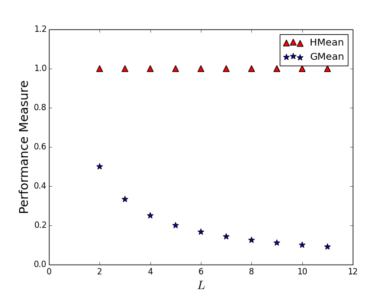
(a) Balanced confusion matrix weights.

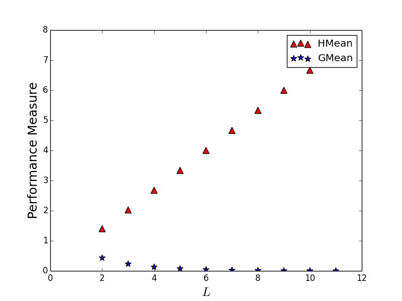
(b) Severely unbalanced confusion matrix weights.

Figure 2: Illustration of H-mean and G-mean performance as the number of classes increases.

8.2 Algorithmic Fairness Definitions

In this section, we discuss how certain statistical definitions from the algorithmic fairness literature can be written in terms of constrained group-objective optimization. The first two – equalized odds and demographic parity – are used for ensuring some notion of fairness in classification and the third – Gini index of inequality – can be used for income analysis of inequality amongst subgroups of a population.

For the first two definitions, the setup is as follows: The goal is to learn an accurate classifier $h:\mathcal{X}\rightarrow\{0,1\}$ from some family of classifiers (e.g., decision trees, neural networks, or polynomial threshold functions) while satisfying some definition of statistical fairness. We assume that we are given training examples $D=\{(\text{{x}}_{i},a_{i},y_{i})\}_{i=1}^{n}\in(\mathcal{X},\mathcal{A},\mathcal{Y})^{n}$ typically representing $n$ individuals drawn i.i.d. over the joint distribution $(\text{{x}},a,y)\sim\mu$. For each $i\in[n]$, $\text{{x}}_{i}\in\mathcal{X}$ is the features of individual $i$, $a_{i}\in\mathcal{A}$ is the protected attribute of the individual (e.g., race or gender), $y_{i}\in\mathcal{Y}$ is the label. Using constrained group-objective optimization, the chosen hypothesis $h$ need not have access to nor knowledge of the protected attribute $A$ during testing or deployment.

Definition 8.4 (Equalized Odds (Hardt et al., 2016)).

A classifier $h$ satisfies Equalized Odds under a distribution over $(\text{{x}},a,y)$ if $h(X)$, its prediction, is conditionally independent of the protected attribute $A$ given the label $Y$.

In notation, we have that for all $a\in\mathcal{A},\hat{y}\in\mathcal{Y},x\in\mathcal{X}$

$$\mathbb{P}_{(\text{{x}},a,y)\sim\mu}\left[h(\text{{x}})=\hat{y}|A=a,Y=y\right]=\mathbb{P}\left[h(\text{{x}})=\hat{y}|Y=y\right].$$

Definition 8.5 (Demographic Parity (Agarwal et al., 2018)).

A classifier $h$ satisfies Demographic Parity under a distribution over $(\text{{x}},a,y)$ if $h(X)$, its prediction, is statistically independent of the protected attribute $A$.

In notation, we have that for all $a\in\mathcal{A},\hat{y}\in\mathcal{Y}$

$$\mathbb{P}_{(\text{{x}},a,y)\sim\mu}\left[h(\text{{x}})=\hat{y}|A=a\right]=\mathbb{P}\left[h(\text{{x}})=\hat{y}\right].$$

For optimization purposes, we often cannot satisfy either equalized odds or demographic parity exactly so we must instead pursue relaxations of equalized odds and demographic parity. For example, Jagielski et al. (2018) pursue $\gamma$ Equalized Odds which is defined in Definition 8.7, stated in terms of false positives and false negatives of a hypothesis $h$.

Definition 8.6 (Gini Index of Inequality (Busa-Fekete et al., 2017)).

Suppose there are $K$ subgroups in a population of individuals earning income. The Gini Index of Inequality is given by

$$I(l)=\frac{\sum_{i,j}|l_{i}-l_{j}|}{2n\sum_{i}l_{i}}\in[0,1],$$

where $l\in[0,1]^{K}$ and $l_{i}$ could represent the percentile average income of individuals in subgroup $i$.

The Gini index is not convex but quasi-convex which means that its level sets are convex. For any given $\theta\in[0,1]$, $I(l)\leq\theta$ is equivalent to

$$\sum_{i,j}|l_{i}-l_{j}|-2n\theta\sum l_{i}\leq 0,$$

which is a convex constraint (Alabi et al., 2018).

Definition 8.6 makes no distributional assumptions on the loss vector $l\in[0,1]^{K}$.

Agarwal et al. (2018) show how to convert the empirical risk minimization problem for satisfying either demographic parity or equalized odds into the following problem:

$$\min_{h\in\Delta}\hat{err}(h)\,\,\text{ s.t. }\,\,M\hat{\mu}(h)\leq\hat{c}$$ (11)

where the matrix $M\in{\mathbb{R}}^{|\mathcal{K}|\times|\mathcal{J}|}$ and the vector $\hat{c}\in{\mathbb{R}}^{|\mathcal{K}|}$ specify linear constraints for the problem and $\hat{\mu}(h)\in{\mathbb{R}}^{|\mathcal{J}|}$ is a vector of conditional moments taken over the the distribution on $(\mathcal{X},A,\mathcal{Y})$.

To convert into the form of constrained group-objective optimization, we set $f(\ell(h,D))=\hat{err}(h)$ and $g(\ell(h,D))=(M\hat{\mu}(h)-\hat{c})\cdot\textbf{1}$ where 1 is the all-ones vector or $g(\ell(h,D))=\max_{i\in[\mathcal{K}]}(M\hat{\mu}(h)-\hat{c})_{i}$. We leave out details of how to convert the definition of Demographic Parity and Equalized Odds into Equation 11 as this is already done in Section 2 (termed “Problem Formulation”) in  (Agarwal et al., 2018). Last, for the Gini index of inequality, we can convert into constrained group-objective optimization by setting the constraint function $g$ to $g(l)=\sum_{i,j}|l_{i}-l_{j}|-2n\theta\sum l_{i}\leq 0$ for some $\theta\in[0,1]$ and setting $f(l)=-\sum_{i}l_{i}$ for all $l\in[0,1]^{K}$.

We note here that $K$, the number of groups, is not a constant and could vary depending on the context, application, and matters of intersectionality (Buolamwini and Gebru, 2018; Hébert-Johnson et al., 2018).

8.2.1 Satisfying Equalized Odds

Now, we show how to satisfy approximate notions of equalized odds while respecting differential privacy constraints.

Definition 8.7 ($\alpha$-Equalized Odds (Jagielski et al., 2018)).

Let $X,A,Y$ be random variables representing the non-sensitive features, the sensitive attribute, and the label assigned to an individual, respectively.

Given a dataset of examples $D=\{(\text{{x}}_{i},a_{i},y_{i})\}_{i=1}^{n}\in(\mathcal{X},\mathcal{A},\{0,1\})^{n}$ of size $n$, we say a classifier $c\in\mathcal{C}_{P}$ satisfies $\alpha$ Equalized Odds if

$$\max_{a,a^{\prime}\in\mathcal{A}}\{\max(|\hat{FP}_{a}-\hat{FP}_{a^{\prime}}|,|\hat{TP}_{a}-\hat{TP}_{a^{\prime}}|)\}\leq\alpha$$ (12)

where $\hat{FP}_{a},\hat{TP}_{a}$ are empirical estimates of $FP_{a}(c)=\mathbb{P}_{(x,y,a)}[c(\text{{x}})=1|A=a,y=0]$, $TP_{a}(c)=\mathbb{P}_{(x,y,a)}[c(\text{{x}})=1|A=a,y=1]$ respectively on dataset $D$.

We say a classifier satisfies $\alpha$-Smoothed Equalized Odds if the smoothed version of Equation 13 is satisfied (i.e., when the maximum and absolute functions in Equation 13 are replaced with smoothed versions or using the Moreau-Yosida regularization technique).

For concreteness, we provide a specific smoothed version of $\alpha$-equalized odds in Definition 8.8.

Definition 8.8 ($(\alpha,\eta)$-Smoothed Equalized Odds).

Let $X,A,Y$ be random variables representing the non-sensitive features, the sensitive attribute, and the label assigned to an individual, respectively.

Given a dataset of examples $D=\{(\text{{x}}_{i},a_{i},y_{i})\}_{i=1}^{n}\in(\mathcal{X},\mathcal{A},\{0,1\})^{n}$ of size $n$, we say a classifier $c\in\mathcal{C}_{P}$ satisfies $(\alpha,\eta)$ Equalized Odds if the constraint function

$$g(\hat{FP},\hat{FN},\hat{TP})=\operatorname*{smax}^{\eta}_{a,a^{\prime}\in\mathcal{A}}\{\max(|\hat{FP}_{a}-\hat{FP}_{a^{\prime}}|,|\hat{TP}_{a}-\hat{TP}_{a^{\prime}}|)\}-\alpha$$ (13)

is less than or equal to 0. $(\hat{FP},\hat{FN},\hat{TP})$ corresponds to the $3|\mathcal{A}|$ empirical estimates of the false positives, false negatives, and true positives for the $|\mathcal{A}|$ groups. $(\hat{FP},\hat{TP})$ are used to enforce the equalized odds constraint while $(\hat{FP},\hat{FN})$ are used to compute the error of the classifier. We use the smooth maximum function $\operatorname*{smax}^{\eta}(y_{1},\ldots,y_{n})=\frac{\sum_{i=1}^{n}y_{i}e^{\eta y_{i}}}{\sum_{i=1}^{n}e^{\eta y_{i}}}$ (Lange et al., 2014). As $\eta\rightarrow\infty$, $\operatorname*{smax}^{\eta}\rightarrow\max$.

Corollary 8.9.

For any privacy parameters $\epsilon,\delta\in(0,1]$, suppose we have a dataset of examples $D=\{(\text{{x}}_{i},a_{i},y_{i})\}_{i=1}^{n}$ of size $n$ where $\text{{x}}_{i}\in\mathcal{X},y_{i}\in\{0,1\}$, $a_{i}\in\mathcal{A}$, for all $i\in[n]$. Assume that there exists at least one decision in $\mathcal{C}_{P}$ (with VC dimension $\operatorname*{VC}(\mathcal{C}_{P})$ in parametric space ${\mathbb{R}}^{P}$) that satisfies $(\alpha,\eta)$-Smoothed Equalized Odds (by Definition 8.7) for some $\eta>0$.

Then there exists $n_{0}=\tilde{O}\left(\frac{|\mathcal{A}|^{4}\cdot\operatorname*{VC}(\mathcal{C}_{P})}{\epsilon\alpha^{3}}\right)$ such that for all $n\geq n_{0}$, with probability at least $9/10$, we can obtain a decision $\tilde{c}\in\mathcal{C}_{P}$ satisfying $(\alpha,\eta)$-smoothed equalized odds and that is within $\alpha$ away from the most accurate classifier.

Proof.

For any classifier $c\in\mathcal{C}_{P}$ we set the loss vector of $c$ on $D$ to

$$\ell(c,D)=(\ell_{1}(c,D),\ldots,\ell_{K}(c,D)),$$

with $K=3|\mathcal{A}|$ where

$$\ell_{1}(c,D)=\hat{FP}_{1},\ldots,\ell_{|A|}(c,D)=\hat{FP}_{|\mathcal{A}|},$$

$$\ell_{|\mathcal{A}|+1}(c,D)=\hat{TP}_{1},\ldots,\ell_{2|A|}(c,D)=\hat{TP}_{|\mathcal{A}|},$$

and

$$\ell_{2|\mathcal{A}|+1}(c,D)=\hat{FN}_{1},\ldots,\ell_{3|A|}(c,D)=\hat{FN}_{|\mathcal{A}|}.$$

Then the empirical error of any classifier $c\in\mathcal{C}_{P}$ is $f(\ell(c,D))=\sum_{a\in\mathcal{A}}\hat{FP}_{a}+\hat{FN}_{a}$ (the sum of the false positives and false negatives) and the $\alpha$-equalized odds is enforced via

$$g(\ell(c,D))=\max_{a,a^{\prime}\in\mathcal{A}}\{\max(|\hat{FP}_{a}-\hat{FP}_{a^{\prime}}|,|\hat{TP}_{a}-\hat{TP}_{a^{\prime}}|)\}-\alpha,$$

so that $g(\ell(c,D))\leq 0$ for all classifiers $c\in\mathcal{C}_{P}$ that satisfy $\alpha$-equalized odds. We use a smoothed version of $g(\ell(c,D))$ (i.e., replace the maximum and absolute functions in that equation with the smooth approximations of those functions or using the Moreau-Yosida regularization technique).

Now, assuming there exists at least one choice $c\in\mathcal{C}_{P}$ such that $g(\ell(c,D))\leq 0$, we can just directly apply Corollary 5.11 to $f,g$ to obtain the desired corollary. ∎

Corollary 8.9 results in sample size $\tilde{O}\left(\frac{|\mathcal{A}|^{4}\cdot\operatorname*{VC}(\mathcal{C}_{P})}{\epsilon\alpha^{3}}\right)$. As a result, the linear optimization based algorithm for Theorem 5.9 performs better (in terms of asymptotic sample complexity) than the DP-oracle-learner of Jagielski et al. (2018) which requires sample size $\tilde{O}\left(\frac{|\mathcal{A}|^{3}\operatorname*{VC}(\mathcal{C}_{P})}{\epsilon\alpha^{3+r}}\right)$ for any $r>0$ provided that $\min_{a,y}\{\hat{q}_{ay}\}\leq\alpha^{(1+r)/2}$ where $\hat{q}_{ay}$ is the empirical estimate of $\mathbb{P}[A=a,Y=y]$.

Example 8.10 shows how to use Corollary 8.9 on specific smooth approximations to the absolute value and maximum functions. Note that this is one of many ways to apply smoothing and this specific version might not apply optimal smoothing. Smoothing of non-smooth functions for specific tasks is an entire research agenda (e.g., see (Bach et al., 2012; Lange et al., 2014) for smooth approximations to the max and absolute value functions) and not the focus of this research paper.

Example 8.10.

Suppose we have two groups and can obtain empirical estimates of the false positive, false negative, and true positive rates of these groups for any $c\in\mathcal{C}_{P}$ and fixed dataset of labeled examples $D=\{(\text{{x}}_{i},a_{i},y_{i})\}_{i=1}^{n}\in(\mathcal{X}\times\{1,2\}\times\{0,1\})^{n}$. The goal is to perform binary classification under $(\alpha,\eta)$ equalized odds constraints. We let $\mathcal{C}_{P}$ be the set of single-parametric threshold classifiers over the reals so that $\operatorname*{VC}(\mathcal{C}_{P})=1$. The loss vector is

$$\ell(c,D)=(\hat{FP}_{1}(c,D),\hat{FP}_{2}(c,D),\hat{FN}_{1}(c,D),\hat{FN}_{2}(c,D),\hat{TP}_{1}(c,D),\hat{TP}_{2}(c,D)).$$

The “error” function $f$ can be computed as the linear function $f(\ell(c,D))=\hat{FP}_{1}(c,D)+\hat{FP}_{2}(c,D)+\hat{FN}_{1}(c,D)+\hat{FN}_{2}(c,D)$ and so is Lipschitz, smooth.

Now, define a smooth approximation to the max function as $\operatorname*{smax}^{\eta}(y_{1},\ldots,y_{n})=\frac{\sum_{i=1}^{n}y_{i}e^{\eta y_{i}}}{\sum_{i=1}^{n}e^{\eta y_{i}}}$. Then if for all decisions $c\in\mathcal{C}_{P}$ and for a fixed $\eta,D$, $\operatorname*{smax}^{\eta}(|\hat{FP}_{1}(c,D)-\hat{FP}_{2}(c,D)|),|\hat{TP}_{1}(c,D)-\hat{TP}_{2}(c,D)|)$ is 1-Lipschitz, we can apply Corollary 8.9 to obtain the desired guarantees.

More generally, the possible empirical rates for any given dataset depends on how complex the decision set $\mathcal{C}_{P}$ is. The decision set $\mathcal{C}_{P}$ could represent all possible parameterizations of a specific neural network architecture, all possible weights for a polynomial threshold function to be used for classification, or a constant separator threshold defined over the reals.

Remark 8.11.

We have shown how to apply our methods to satisfy certain statistical definitions of algorithmic fairness and some convex performance measures of the confusion matrix. There are potentially other use cases we have not explored that we leave for future work.

9 Conclusion

In this paper, we have explored the problem of private fair optimization via a reductions approach. We provided an $(\epsilon,0)$-differentially private exponential sampling algorithm and an $(\epsilon,\delta)$-differentially private linear optimization based algorithm as a solution. As a side-effect perhaps, we introduce a class of bounded divergence linear optimizers, which could be useful for solving more general (Lipschitz-continuous) multi-objective problems. We also provide a lower bound on the excess risk (or equivalently, on the sample complexity) for any $\epsilon$ or $(\epsilon,\delta)$-differentially private algorithm that solves the constrained group-objective optimization problem.

Our framework can also be used to solve model projection (Alghamdi et al., 2020) for certain constraint sets constructed via linear inequalities. Constructively showing connections between the model projection problem (for certain $f$-divergences) and linear optimizers with divergence constraints is left to future work. Furthermore, linear optimizers share the same form as a Rectified Linear Unit (ReLU) used in deep learning. Showing constructive equivalences, especially by delineating time/accuracy tradeoffs (Goel et al., 2019), is left to future work.

10 Acknowledgements

Thanks to Salil Vadhan for providing detailed comments on this paper at various stages of the project and to Cynthia Dwork, Adam Smith, and other members of the Boston-Area Data Privacy group for comments that improved the writing of this work. We are grateful to Shahab Asoodeh, Boaz Barak, Flavio du Pin Calmon, Nicole Immorlica, Adam Tauman Kalai, Sanmi Koyejo, Ankur Moitra, Jelani Nelson, and Chris Wiggins for illuminating discussions related to this work. The Computational Social Science group at Facebook AI Research and participants of the “Recent Themes in Resource Tradeoffs: Privacy, Fairness, and Robustness” workshop at the University of Minnesota provided many helpful comments and suggestions that improved the writing of this work. Finally, we appreciate the guidance of the anonymous referees who helped to improve the presentation of this work.

Appendix A Some Inequalities and Advanced Composition Result

Lemma A.1 (Markov’s Inequality).

Let $Z$ be a non-negative random variable. Then for all $a\geq 0$,

$$\mathbb{P}[Z\geq a]\leq\frac{\mathbb{E}[Z]}{a},$$

where $\mathbb{E}[Z]=\int_{x=0}^{\infty}\mathbb{P}[Z\geq x]dx$.

Lemma A.2 (Cauchy-Schwarz Inequality).

For any two vectors $\mathbf{u},\mathbf{v}$ of an inner product space we have that

$$|\langle\mathbf{u},\mathbf{v}\rangle|\leq\mathopen{\|}\mathbf{u}\mathclose{\|}\mathopen{\|}\mathbf{v}\mathclose{\|}.$$

Lemma A.3 (Jensen’s Inequality).

For any $t\in[0,1]$ and convex function $f:\mathcal{X}\rightarrow{\mathbb{R}}$, the following holds:

$$f(t\text{{x}}_{1}+(1-t)\text{{x}}_{2})\leq tf(\text{{x}}_{1})+(1-t)f(\text{{x}}_{2}),$$

for any $\text{{x}}_{1},\text{{x}}_{2}\in\mathcal{X}$.

Lemma A.4 (Advanced Composition (Dwork et al. [2010])).

For all $\epsilon,\delta,\bar{\delta}\geq 0$, the class of $(\epsilon,\delta)$-differentially private mechanisms results in $(\bar{\epsilon},k\delta+\bar{\delta})$-differential privacy under $k$-fold adaptive composition for:

$$\bar{\epsilon}=\epsilon\sqrt{2k\log(1/\bar{\delta})}+k\epsilon(e^{\epsilon}-1).$$

A corollary of Lemma A.4 states that we can set $\epsilon=\frac{\bar{\epsilon}}{2\sqrt{2k\log(1/\bar{\delta})}}$ to ensure $(\bar{\epsilon},k\delta+\bar{\delta})$ differential privacy overall for target privacy parameters $\bar{\epsilon}\in(0,1),\bar{\delta}\in(0,1]$.

Appendix B Projection-Free Convex Optimization using Frank-Wolfe

In previous sections, we presented linear optimization based algorithms to solve the constrained group-objective optimization problem with and without privacy. In this section, we present another linear optimization based algorithm that is an adaptation of the Frank-Wolfe projection-free algorithm. Algorithm 3 is the Frank-Wolfe algorithm presented in  [Jaggi, 2013] which allows for use of approximate linear optimizers to solve the subproblems in each iteration $t\in[T]$. The original version of Frank-Wolfe only allowed for exact linear optimizers.

Lemma B.2 presents the convergence guarantees of the algorithm after $k$ iterations in terms of the curvature constant of the function $h:{\mathbb{R}}^{K}\rightarrow{\mathbb{R}}$ to be optimized (see Definition B.1) and the accuracy of the linear optimizer oracle. We will rely on a modified version of Algorithm 3 to solve the constrained group-objective optimization problem (Definition 1.2).

The execution of Algorithm 3 in each iteration relies on the availability of an approximate linear oracle of the form $\min_{\hat{s}\in\mathcal{C}}\langle\hat{s},\nabla h(y^{(t)})\rangle$. In [Alabi et al., 2018], the authors provide an algorithm that can optimize any Lipschitz-continuous function $h:{\mathbb{R}}^{K}\rightarrow{\mathbb{R}}$ using an approximate linear optimizer as an oracle solver.

1Let $y^{(0)}\in\mathcal{C}$

2for $t=0,\dots,T$ do

3       Let $\gamma=\frac{2}{t+2}$

4      Find $s\in\mathcal{C}$ s.t. $\langle s,\nabla h(y^{(t)})\rangle\leq\min_{\hat{s}\in\mathcal{C}}\langle\hat{s},\nabla h(y^{(t)})\rangle+\frac{1}{2}\rho\gamma C_{h}$

5      Update $y^{(t+1)}=(1-\gamma)y^{(t)}+\gamma s$

6

Algorithm 3 Frank-Wolfe algorithm [Jaggi, 2013]

For the results in this paper that rely on solving approximate linear subproblems, $y^{(t)}$ in Algorithm 3 would correspond to the $K$-dimensional loss vector $\ell(c,D)\in[0,1]^{K}$ defined for a decision $c\in\mathcal{C}_{P}$ on dataset $D$ of size $n$.

Definition B.1.

The curvature constant $C_{h}$ of a convex and differentiable function $h:{\mathbb{R}}^{K}\rightarrow{\mathbb{R}}$, with respect to a compact domain $\mathcal{C}$ is defined as

$$C_{h}=\sup_{x,s\in\mathcal{C},\gamma\in[0,1],y=x+\gamma(s-x)}\frac{2}{\gamma^{2}}\left(h(y)-h(x)-\langle y-x,\nabla h(x)\rangle\right),$$

where $\nabla h$ is the gradient of the function $h$.

Lemma B.2.

Let $h:\mathcal{C}\rightarrow{\mathbb{R}}$ be any convex function, then using the Frank-Wolfe algorithm (Algorithm 3), we have that for any $t\geq 1$ and iterates $y^{(t)},$

$$h(y^{(t)})-h(y^{*})\leq\frac{2C_{h}}{t+2}(1+\rho),$$

where $y^{*}\in\operatorname*{argmin}_{y\in\mathcal{C}}h(y)$, $\rho\geq 0$ is the accuracy to which the internal linear subproblems are solved, and $C_{h}$ is the curvature constant of the function $h$.

Lemma B.3.

Let $h$ be a convex and differentiable Lipschitz-continuous function with gradient $\nabla h$ w.r.t. some norm $\mathopen{\|}\cdot\mathclose{\|}$ over domain $\mathcal{C}$. If $\nabla h$ has Lipschitz constant $\beta_{h}>0$, then

$$C_{h}\leq\operatorname*{diam}_{\mathopen{\|}\cdot\mathclose{\|}}(\mathcal{C})^{2}\beta_{h},$$

where $\operatorname*{diam}_{\mathopen{\|}\cdot\mathclose{\|}}(\mathcal{C})$ is the diameter of $\mathcal{C}$.

Now we describe how to solve constrained group objective optimization using the Frank-Wolfe algorithm as opposed to the algorithm of  Alabi et al. [2018].

B.1 Frank-Wolfe Algorithm for Constrained Group-Objective Optimization

In this section, we present a projection-free algorithm based on Frank-Wolfe that solves the constrained group-objective optimization problem without privacy considerations.

In each iteration $t\in[T]$, Algorithm 4 solves the following linear sub-problem

$$c_{t+1}=\operatorname*{argmin}_{c\in\mathcal{C}_{P}}\langle\,\,(\nabla f(\ell(c_{t},D))+G\cdot\mathds{1}[g(\ell(c_{t},D))\geq 0]\cdot\nabla g(\ell(c_{t},D))),\ell(c,D)\,\,\rangle,$$

and then “moves” towards $c_{t+1}$ by a multiplicative factor of $\frac{2}{t+2}$. We show that after $T=O\left(\frac{K\sqrt{K}}{\alpha^{2}}\log\frac{K\sqrt{K}}{\alpha^{2}}\right)$ iterations we will get a decision $\hat{c}$ that is within $\alpha$ (in terms of $f,g$) of the optimal decision $c^{*}\in\operatorname*{argmin}_{c\in\mathcal{C}_{P}:g(\ell(c,D))\leq 0}f(\ell(c,D))$. The function $\text{Unif}(\{c_{1},\ldots,c_{T}\})$ returns $\hat{c}$ that predicts with decision $c_{i}$ with probability $\frac{1}{T}$ for any $i\in[T]$.

1

Input: $\operatorname*{argmin}_{\mathcal{C}_{P}}\langle\cdot,\cdot\rangle,T,\ell,\nabla f,\nabla g,D\in(\mathcal{X}\times\mathcal{A}\times\mathcal{Y})^{n},G$

2

3 

4Pick any decision $c\in\mathcal{C}_{P}$ as $c_{1}$ with $l_{1}(D)=\ell(c,D)$

5 

6for $t=1,\ldots,T-1$ do

7      

8      $c_{t+1}=\operatorname*{argmin}_{c\in\mathcal{C}_{P}}\langle\,\,\ell(c,D),(\nabla f(\ell(c_{t},D))+G\cdot\mathds{1}[g(\ell(c_{t},D))\geq 0]\cdot\nabla g(\ell(c_{t},D)))\,\,\rangle$

9      $l_{t+1}(D)=\left(1-\frac{2}{t+2}\right)l_{t}(D)+\frac{2}{t+2}\ell(c_{t+1},D)$

10

11 

return $\hat{c}=\text{Unif}(\{c_{1},\ldots,c_{T}\})$

Algorithm 4 Frank-Wolfe algorithm for Constrained Group-Objective Convex Optimization.

Lemma B.4.

Suppose we are given convex, smooth functions $f,g:[0,1]^{K}\rightarrow{\mathbb{R}}$ and loss function $\ell:\mathcal{C}_{P}\times(\mathcal{X}\times\mathcal{A}\times\mathcal{Y})^{n}\rightarrow[0,1]^{K}$. Then for any setting of $G>0,T\geq 3$, Algorithm 4 returns a decision $\hat{c}\in\mathcal{C}_{P}$ with the following guarantee:

$$\mathbb{E}[f(\ell(\hat{c},D))]\leq f(\ell(c^{*},D))+\frac{2K(\beta_{f}+G\beta_{g})\log T}{T},\quad\quad\mathbb{E}[g(\ell(\hat{c},D))]\leq\frac{2K(\beta_{f}+G\beta_{g})\log T}{T}\cdot\frac{1}{G}+\frac{\sqrt{K}}{G},$$

where $c^{*}\in\operatorname*{argmin}_{c\in\mathcal{C}_{P}:g(\ell(c,D))\leq 0}f(\ell(c,D))$ is the best decision in the feasible set $\mathcal{C}_{P}$, $D$ is a dataset of size $n$, $\beta_{f}$ is the smoothness parameter of the function $f$ and $\beta_{g}$ is the smoothness parameter of the function $g$. This result holds assuming access to a linear optimizer oracle.

Proof.

The intuition is to optimize w.r.t. a “new” convex, smooth function $h(\ell(c,D))=f(\ell(c,D))+G\cdot\max(0,g(\ell(c,D)))$ for any $c\in\mathcal{C}_{P}$ and dataset $D$. We rely on the primal convergence guarantees of the Frank-Wolfe algorithm. By Lemma B.2, we have that in iteration $t\geq 1$, the following holds:

$$h(\ell(c_{t},D))\leq h(\ell(c^{*},D))+\frac{2C_{h}}{t+2},$$

where $C_{h}$ is the curvature constant of $h$. And by Lemma B.3, we have $C_{h}\leq K(\beta_{f}+G\beta_{g})$ where $(\beta_{f}+G\beta_{g})$ is the smoothness parameter of the function $h$. As a result we have that $h(\ell(c_{t},D))\leq h(\ell(c^{*},D))+\frac{2K(\beta_{f}+G\beta_{g})}{t+2}$.

Then by Jensen’s inequality (Lemma A.3) and convexity of $h\circ\ell$, we have

$$\mathbb{E}_{c\sim\{c_{i}\}_{i=1}^{T}}[h(\ell(c,D))] \leq\frac{1}{T}\sum_{t=1}^{T}h(\ell(c_{t},D))$$ (14)

$$\leq h(\ell(c^{*},D))+\frac{2K(\beta_{f}+G\beta_{g})}{T}\left(\frac{1}{3}+\frac{1}{4}+\frac{1}{5}+\ldots+\frac{1}{T+2}\right)$$ (15)

$$\leq h(\ell(c^{*},D))+\frac{2K(\beta_{f}+G\beta_{g})\log T}{T}$$ (16)

where we used that the harmonic number $H_{T}$ is upper bounded by $\log T+1$ and that $\frac{1}{T+1}+\frac{1}{T+2}<1/2$ for $T\geq 3$.

We apply Lemma 4.1 to obtain that $\mathbb{E}[f(\ell(\hat{c},D))]\leq f(\ell(c^{*},D))+\frac{2K(\beta_{f}+G\beta_{g})\log T}{T}$ and $\mathbb{E}[g(\ell(\hat{c},D))]\leq\frac{2K(\beta_{f}+G\beta_{g})\log T}{T}\cdot\frac{1}{G}+\frac{\sqrt{K}}{G}$. ∎

Corollary B.5.

Suppose we are given convex, smooth functions $f,g:[0,1]^{K}\rightarrow{\mathbb{R}}$ and loss function $\ell:\mathcal{C}_{P}\times(\mathcal{X}\times\mathcal{A}\times\mathcal{Y})^{n}\rightarrow[0,1]^{K}$. Let $\beta_{f},\beta_{g}$ be the Lipschitz constants of the gradients of $f,g$ respectively. Then for any setting of $T\geq 3,\alpha>0$, Algorithm 4 returns a decision $\hat{c}\in\mathcal{C}_{P}$ with the following guarantee:

$$\mathbb{E}[f(\ell(\hat{c},D))]\leq f(\ell(c^{*},D))+\alpha,\text{ and }\mathbb{E}[g(\ell(\hat{c},D))]\leq\alpha,$$

provided that $G\geq\frac{\alpha+\sqrt{K}}{\alpha}$ and $T\geq\frac{2K(\beta_{f}+G\beta_{g})}{\alpha}\log\frac{2K(\beta_{f}+G\beta_{g})}{\alpha}$ where $c^{*}\in\operatorname*{argmin}_{c\in\mathcal{C}_{P}:g(\ell(c,D))\leq 0}f(\ell(c,D))$ is the best decision in the feasible set $\mathcal{C}_{P}$, $D$ is a dataset of size $n$, $\beta_{f}$ is the smoothness parameter of the function $f$ and $\beta_{g}$ is the smoothness parameter of the function $g$. This result holds assuming access to a linear optimizer oracle.

Proof.

The corollary follows by applying Lemmas 4.2 and B.4 where we set $G\geq\frac{\alpha+\sqrt{K}}{\alpha}$ and

$$T\geq\frac{2K(\beta_{f}+G\beta_{g})}{\alpha}\log\frac{2K(\beta_{f}+G\beta_{g})}{\alpha}$$

in Algorithm 4. ∎

We adapted the Frank-Wolfe algorithm to solve the constrained group-objective optimization problem (via calls to a linear optimizer). Given the versatility of (stochastic) gradient descent, we could also solve the problem via the use of gradient descent. For example, Theorem 3.7 from [Bubeck, 2015] gives guarantees for projected gradient descent optimization of convex, smooth functions. And Theorem 2 from Shamir and Zhang [2013] gives guarantees for convex (but not necessarily smooth) functions.

Appendix C Using a Private Cost Sensitive Classification Oracle $\operatorname*{CSC}_{\epsilon^{\prime}}$

Agarwal et al. [2018] present an exponentiated gradient algorithm for fair classification. Jagielski et al. [2018] essentially modify this algorithm, making it differentially private, and term the new algorithm DP-oracle-learner. DP-oracle-learner satisfies $(\epsilon,\delta)$-differential privacy relying on a private cost sensitive classification oracle $\operatorname*{CSC}_{\epsilon^{\prime}}(\mathcal{H})$ in each iteration where $\epsilon^{\prime}=\frac{\epsilon}{4\sqrt{T\log(1/\delta)}}$ and $\mathcal{H}$ is the hypothesis class to be learned.

DP-oracle-learner solves the $\gamma$-fair empirical risk minimization (ERM) problem given by:

$\min_{Q\in\Delta(\mathcal{H})}\hat{\mathrm{err}}(Q)$
s.t. $\forall\,0\neq a\in\mathcal{A}$: $\Delta\hat{FP}_{a}(Q)=|\hat{FP}_{a}(Q)-\hat{FP}_{0}(Q)|\leq\gamma$,   $\Delta\hat{TP}_{a}(Q)=|\hat{TP}_{a}(Q)-\hat{TP}_{0}(Q)|\leq\gamma$

where $\hat{FP}_{a}(Q),\hat{TP}_{a}(Q)$ are empirical estimates of $FP_{a}(Q)=\mathbb{P}_{(x,y,a)}[Q(x)=1|A=a,y=0]$, $TP_{a}(Q)=\mathbb{P}_{(x,y,a)}[Q(x)=1|A=a,y=1]$ respectively and group 0 is used as an anchor. $\mathcal{A}$ is the set of labels for all protected/sensitive attributes and $A$ is the random variable over $\mathcal{A}$.

Agarwal et al. [2018] solve the following specific Lagrangian min-max problem:

$$\min_{Q\in\Delta(\mathcal{H})}\max_{\bm{\lambda}\in\Lambda}L(Q,\bm{\lambda})=\hat{\mathrm{err}}(Q)+\bm{\lambda}^{T}\hat{\bm{r}}(Q),$$

where $\Delta(\mathcal{H})$ is the set of all randomized classifiers that can be obtained by hypotheses in $\mathcal{H}$, $\hat{\bm{r}}(Q)$ is a vector representing the fairness violations of the classifier $Q$ across all groups, $\bm{\lambda}\in\Lambda=\{\bm{\lambda}:\mathopen{\|}\bm{\lambda}\mathclose{\|}_{1}\leq B\}$, and the bound $B$ is chosen to ensure convergence.

Now we state a main theorem from [Jagielski et al., 2018].

Theorem C.1 (Theorem 4.4 from [Jagielski et al., 2018]).

Let $(\tilde{Q},\tilde{\bm{\lambda}})$ be the output of DP-oracle-learner, an $(\epsilon,\delta)$-differentially private algorithm, in  [Jagielski et al., 2018] and let $Q^{*}$ be a solution to the non-private $\gamma$-fair ERM problem (see above definition). Then with probability at least $0.99,$

$$\hat{\mathrm{err}}(\tilde{Q})\leq\hat{\mathrm{err}}(Q^{*})+2\nu,$$

and for all $a\neq 0$,

$$\Delta\hat{FP}_{a}(\tilde{Q})\leq\gamma+\frac{1+2\nu}{B},$$

$$\Delta\hat{TP}_{a}(\tilde{Q})\leq\gamma+\frac{1+2\nu}{B},$$

where $\nu=\tilde{O}\left(\frac{B}{\min_{a,y}\hat{q}_{ay}}\sqrt{\frac{|\mathcal{A}|\cdot\operatorname*{VC}(\mathcal{H})}{n\epsilon}}\right),$ $n$ is the number of training examples $\{(\text{{x}}_{i},a_{i},y_{i})\}^{n}_{i=1}$ fed to the Algorithm, $\operatorname*{VC}(\mathcal{H})$ is the VC dimension of $\mathcal{H}$, and $\hat{q}_{ay}$ is an empirical estimate for $\mathbb{P}[A=a,Y=y]$.

As is done in their paper, to get rid of the algorithmic-specific dependence on the bound $B$ (for example, in Theorem 4.6 of their paper), we set $B=|\mathcal{A}|$.

Corollary C.2.

Let $(\tilde{Q},\tilde{\bm{\lambda}})$ be the output of Algorithm 3, an $(\epsilon,\delta)$-differentially private algorithm, in  [Jagielski et al., 2018] and let $Q^{*}$ be a solution to the non-private $\alpha$-fair ERM problem (see above definition) where $\min_{a,y}\{\hat{q}_{ay}\}\leq\alpha^{(1+r)/2}$ for any $r>0$. Then with probability at least 9/10, in order to solve the ERM problem with classifier error $\alpha=(\hat{\mathrm{err}}(\tilde{Q})-\hat{\mathrm{err}}(Q^{*}))$ and maximum fairness violation of $\alpha=\max_{a\in\mathcal{A}}\max(\Delta\hat{FP}_{a}(\tilde{Q}),\Delta\hat{TP}_{a}(\tilde{Q}))$, we could use training examples of size

$$n=\tilde{O}\left(\frac{|\mathcal{A}|^{3}\cdot\operatorname*{VC}(\mathcal{H})}{\epsilon\alpha^{3+r}}\right).$$

Proof.

Set $\min_{a,y}\{\hat{q}_{ay}\}\leq\alpha^{(1+r)/2}$ in Theorem C.1. ∎

Corollary C.2 is obtained directly from Theorem C.1 by solving for $n$ in terms of the excess risk and will be used as the point of comparison to compare our work to the work of Jagielski et al. [2018] for solving the $\alpha$-fair ERM problem (for the Equalized Odds problem) with classifier error of $\alpha$ with probability at least 9/10. Further note that $K=O(|\mathcal{A}|)$ is the number of groups (in terminology used in other parts of this paper). A result of this corollary is that to solve the $\textrm{CGOO}(\mathcal{C}_{P},n,K,f,g,\ell,D,\alpha)$ problem when the constraint is to satisfy $\alpha$-equalized odds, we need sample size $n=\tilde{O}\left(\frac{|\mathcal{A}|^{3}\cdot\operatorname*{VC}(\mathcal{H})}{\epsilon\alpha^{3+r}}\right)$. In comparison, using a generic implementation of the private oracle $\operatorname*{LOPT}_{\epsilon,\delta}$, we need sample size $n=\tilde{O}\left(\frac{|\mathcal{A}|^{4}\cdot\operatorname*{VC}(\mathcal{H})}{\epsilon\alpha^{3}}\right)$ which is asymptotically better (in terms of the accuracy parameter $\alpha>0$) for all $r>0$.

Note that according to Assumption C.1 in [Jagielski et al., 2018], the $\operatorname*{CSC}(\mathcal{H})$ oracle and its private counterpart are often implemented via learning heuristics.

References

- Abowd [2018] John M. Abowd. The u.s. census bureau adopts differential privacy. In Proceedings of the 24th ACM SIGKDD International Conference on Knowledge Discovery & Data Mining, KDD ’18, page 2867, New York, NY, USA, 2018. Association for Computing Machinery. ISBN 9781450355520. URL https://doi.org/10.1145/3219819.3226070.
- Agarwal et al. [2018] Alekh Agarwal, Alina Beygelzimer, Miroslav Dudík, John Langford, and Hanna M. Wallach. A reductions approach to fair classification. In Proceedings of the 35th International Conference on Machine Learning, ICML 2018, Stockholmsmässan, Stockholm, Sweden, July 10-15, 2018, pages 60–69, 2018.
- Agarwal et al. [2019] Alekh Agarwal, Miroslav Dudík, and Zhiwei Steven Wu. Fair regression: Quantitative definitions and reduction-based algorithms. In Proceedings of the 36th International Conference on Machine Learning, ICML 2019, 9-15 June 2019, Long Beach, California, USA, pages 120–129, 2019. URL http://proceedings.mlr.press/v97/agarwal19d.html.
- Alabi et al. [2018] Daniel Alabi, Nicole Immorlica, and Adam Tauman Kalai. Unleashing linear optimizers for group-fair learning and optimization. In Conference On Learning Theory, COLT 2018, Stockholm, Sweden, 6-9 July 2018., pages 2043–2066, 2018. URL http://proceedings.mlr.press/v75/alabi18a.html.
- Alghamdi et al. [2020] Wael Alghamdi, Shahab Asoodeh, Hao Wang, Flávio P. Calmon, Dennis Wei, and Karthikeyan Natesan Ramamurthy. Model projection: Theory and applications to fair machine learning. In IEEE International Symposium on Information Theory, ISIT 2020, Los Angeles, CA, USA, June 21-26, 2020, pages 2711–2716. IEEE, 2020.
- Bach et al. [2012] Francis R. Bach, Rodolphe Jenatton, Julien Mairal, and Guillaume Obozinski. Optimization with sparsity-inducing penalties. Foundations and Trends in Machine Learning, 4(1):1–106, 2012. URL https://doi.org/10.1561/2200000015.
- Ball et al. [2020] Marshall Ball, Elette Boyle, Akshay Degwekar, Apoorvaa Deshpande, Alon Rosen, Vinod Vaikuntanathan, and Prashant Nalini Vasudevan. Cryptography from information loss. In 11th Innovations in Theoretical Computer Science Conference, ITCS 2020, January 12-14, 2020, Seattle, Washington, USA, pages 81:1–81:27, 2020.
- Bartlett et al. [2006] Peter L Bartlett, Michael I Jordan, and Jon D McAuliffe. Convexity, classification, and risk bounds. Journal of the American Statistical Association, 101(473):138–156, 2006. doi: 10.1198/016214505000000907.
- Bassily et al. [2014] Raef Bassily, Adam D. Smith, and Abhradeep Thakurta. Private empirical risk minimization: Efficient algorithms and tight error bounds. In 55th IEEE Annual Symposium on Foundations of Computer Science, FOCS 2014, Philadelphia, PA, USA, October 18-21, 2014, pages 464–473, 2014.
- Bennett et al. [1995] Charles H. Bennett, Gilles Brassard, Claude Crépeau, and Ueli M. Maurer. Generalized privacy amplification. IEEE Trans. Inf. Theory, 41(6):1915–1923, 1995. URL https://doi.org/10.1109/18.476316.
- Beygelzimer et al. [2009] Alina Beygelzimer, John Langford, and Bianca Zadrozny. Tutorial summary: Reductions in machine learning. In Andrea Pohoreckyj Danyluk, Léon Bottou, and Michael L. Littman, editors, Proceedings of the 26th Annual International Conference on Machine Learning, ICML 2009, Montreal, Quebec, Canada, June 14-18, 2009, volume 382 of ACM International Conference Proceeding Series, page 12. ACM, 2009.
- Blackwell [1956] David Blackwell. An analog of the minimax theorem for vector payoffs. Pacific Journal of Mathematics, 6(1):1–8, 1956.
- Blumer et al. [1989] Anselm Blumer, Andrzej Ehrenfeucht, David Haussler, and Manfred K. Warmuth. Learnability and the vapnik-chervonenkis dimension. J. ACM, 36(4):929–965, 1989. URL https://doi.org/10.1145/76359.76371.
- Bousquet and Elisseeff [2000] Olivier Bousquet and André Elisseeff. Algorithmic stability and generalization performance. In Advances in Neural Information Processing Systems 13, Papers from Neural Information Processing Systems (NIPS) 2000, Denver, CO, USA, pages 196–202, 2000. URL https://proceedings.neurips.cc/paper/2000/hash/49ad23d1ec9fa4bd8d77d02681df5cfa-Abstract.html.
- Brassard et al. [1986] Gilles Brassard, Claude Crépeau, and Jean-Marc Robert. Information theoretic reductions among disclosure problems. In 27th Annual Symposium on Foundations of Computer Science, Toronto, Canada, 27-29 October 1986, pages 168–173. IEEE Computer Society, 1986. URL https://doi.org/10.1109/SFCS.1986.26.
- Bubeck [2015] Sébastien Bubeck. Convex optimization: Algorithms and complexity. Foundations and Trends in Machine Learning, 8(3-4):231–357, 2015.
- Buolamwini and Gebru [2018] Joy Buolamwini and Timnit Gebru. Gender shades: Intersectional accuracy disparities in commercial gender classification. In Conference on Fairness, Accountability and Transparency, FAT 2018, 23-24 February 2018, New York, NY, USA, pages 77–91, 2018. URL http://proceedings.mlr.press/v81/buolamwini18a.html.
- Busa-Fekete et al. [2017] Róbert Busa-Fekete, Balázs Szörényi, Paul Weng, and Shie Mannor. Multi-objective bandits: Optimizing the generalized gini index. In Proceedings of the 34th International Conference on Machine Learning, ICML 2017, Sydney, NSW, Australia, 6-11 August 2017, pages 625–634, 2017. URL http://proceedings.mlr.press/v70/busa-fekete17a.html.
- Canonne et al. [2019] Clément L. Canonne, Gautam Kamath, Audra McMillan, Adam D. Smith, and Jonathan Ullman. The structure of optimal private tests for simple hypotheses. In Proceedings of the 51st Annual ACM SIGACT Symposium on Theory of Computing, STOC 2019, Phoenix, AZ, USA, June 23-26, 2019, pages 310–321, 2019.
- Carlini et al. [2019] Nicholas Carlini, Chang Liu, Úlfar Erlingsson, Jernej Kos, and Dawn Song. The secret sharer: Evaluating and testing unintended memorization in neural networks. In Nadia Heninger and Patrick Traynor, editors, 28th USENIX Security Symposium, USENIX Security 2019, Santa Clara, CA, USA, August 14-16, 2019, pages 267–284. USENIX Association, 2019. URL https://www.usenix.org/conference/usenixsecurity19/presentation/carlini.
- Cesa-Bianchi and Lugosi [2006] Nicolò Cesa-Bianchi and Gábor Lugosi. Prediction, learning, and games. Cambridge University Press, 2006.
- Chaudhuri and Hsu [2011] Kamalika Chaudhuri and Daniel J. Hsu. Sample complexity bounds for differentially private learning. In COLT 2011 - The 24th Annual Conference on Learning Theory, June 9-11, 2011, Budapest, Hungary, pages 155–186, 2011. URL http://proceedings.mlr.press/v19/chaudhuri11a/chaudhuri11a.pdf.
- Chaudhuri et al. [2011] Kamalika Chaudhuri, Claire Monteleoni, and Anand D. Sarwate. Differentially private empirical risk minimization. Journal of Machine Learning Research, 12:1069–1109, 2011.
- Chervonenkis and Vapnik [1971] A. Ya. Chervonenkis and V. N. Vapnik. On the Uniform Convergence of Relative Frequencies of Events to Their Probabilities, 1971. ISSN 0040-585X.
- Choromanski and Malkin [2012] Krzysztof Choromanski and Tal Malkin. The power of the dinur-nissim algorithm: breaking privacy of statistical and graph databases. In Proceedings of the 31st ACM SIGMOD-SIGACT-SIGART Symposium on Principles of Database Systems, PODS 2012, Scottsdale, AZ, USA, May 20-24, 2012, pages 65–76, 2012. URL https://doi.org/10.1145/2213556.2213570.
- Consortium et al. [2009] P3G Consortium, George Church, Catherine Heeney, Naomi Hawkins, Jantina de Vries, Paula Boddington, Jane Kaye, Martin Bobrow, and Bruce Weir. Public access to genome-wide data: Five views on balancing research with privacy and protection. PLOS Genetics, 5(10):1–4, 10 2009. URL https://doi.org/10.1371/journal.pgen.1000665.
- Cormode et al. [2018] Graham Cormode, Somesh Jha, Tejas Kulkarni, Ninghui Li, Divesh Srivastava, and Tianhao Wang. Privacy at scale: Local differential privacy in practice. In Proceedings of the 2018 International Conference on Management of Data, SIGMOD ’18, page 1655–1658, New York, NY, USA, 2018. Association for Computing Machinery. ISBN 9781450347037. URL https://doi.org/10.1145/3183713.3197390.
- Cuff and Yu [2016] Paul Cuff and Lanqing Yu. Differential privacy as a mutual information constraint. In Proceedings of the 2016 ACM SIGSAC Conference on Computer and Communications Security, Vienna, Austria, October 24-28, 2016, pages 43–54, 2016.
- De [2012] Anindya De. Lower bounds in differential privacy. In Ronald Cramer, editor, Theory of Cryptography, pages 321–338, Berlin, Heidelberg, 2012. Springer Berlin Heidelberg. ISBN 978-3-642-28914-9.
- Dinur and Nissim [2003] Irit Dinur and Kobbi Nissim. Revealing information while preserving privacy. In Proceedings of the Twenty-second ACM SIGMOD-SIGACT-SIGART Symposium on Principles of Database Systems, PODS ’03, pages 202–210, New York, NY, USA, 2003. ACM. ISBN 1-58113-670-6.
- Donoho [2006] D.L. Donoho. Compressed sensing. IEEE Transactions on Information Theory, 52(4):1289–1306, 2006. doi: 10.1109/TIT.2006.871582.
- Dwork and Lei [2009] Cynthia Dwork and Jing Lei. Differential privacy and robust statistics. In Proceedings of the 41st Annual ACM Symposium on Theory of Computing, STOC 2009, Bethesda, MD, USA, May 31 - June 2, 2009, pages 371–380, 2009.
- Dwork and Roth [2014] Cynthia Dwork and Aaron Roth. The algorithmic foundations of differential privacy. Foundations and Trends in Theoretical Computer Science, 9(3-4):211–407, 2014.
- Dwork et al. [2006] Cynthia Dwork, Frank McSherry, Kobbi Nissim, and Adam D. Smith. Calibrating noise to sensitivity in private data analysis. In Theory of Cryptography, Third Theory of Cryptography Conference, TCC 2006, New York, NY, USA, March 4-7, 2006, Proceedings, pages 265–284, 2006.
- Dwork et al. [2010] Cynthia Dwork, Guy N. Rothblum, and Salil P. Vadhan. Boosting and differential privacy. In 51th Annual IEEE Symposium on Foundations of Computer Science, FOCS 2010, October 23-26, 2010, Las Vegas, Nevada, USA, pages 51–60, 2010.
- Dwork et al. [2012] Cynthia Dwork, Moritz Hardt, Toniann Pitassi, Omer Reingold, and Richard S. Zemel. Fairness through awareness. In Innovations in Theoretical Computer Science 2012, Cambridge, MA, USA, January 8-10, 2012, pages 214–226, 2012.
- Dwork et al. [2015] Cynthia Dwork, Vitaly Feldman, Moritz Hardt, Toniann Pitassi, Omer Reingold, and Aaron Leon Roth. Preserving statistical validity in adaptive data analysis. In Proceedings of the Forty-Seventh Annual ACM on Symposium on Theory of Computing, STOC 2015, Portland, OR, USA, June 14-17, 2015, pages 117–126, 2015.
- Ehrenfeucht et al. [1989] Andrzej Ehrenfeucht, David Haussler, Michael J. Kearns, and Leslie G. Valiant. A general lower bound on the number of examples needed for learning. Inf. Comput., 82(3):247–261, 1989. URL https://doi.org/10.1016/0890-5401(89)90002-3.
- Ekstrand et al. [2018] Michael D. Ekstrand, Rezvan Joshaghani, and Hoda Mehrpouyan. Privacy for all: Ensuring fair and equitable privacy protections. In Conference on Fairness, Accountability and Transparency, FAT 2018, 23-24 February 2018, New York, NY, USA, pages 35–47, 2018. URL http://proceedings.mlr.press/v81/ekstrand18a.html.
- Feldman and Vondrák [2019] Vitaly Feldman and Jan Vondrák. High probability generalization bounds for uniformly stable algorithms with nearly optimal rate. In Alina Beygelzimer and Daniel Hsu, editors, Conference on Learning Theory, COLT 2019, 25-28 June 2019, Phoenix, AZ, USA, volume 99 of Proceedings of Machine Learning Research, pages 1270–1279. PMLR, 2019. URL http://proceedings.mlr.press/v99/feldman19a.html.
- Freund and Schapire [1997] Yoav Freund and Robert E. Schapire. A decision-theoretic generalization of on-line learning and an application to boosting. J. Comput. Syst. Sci., 55(1):119–139, 1997. URL https://doi.org/10.1006/jcss.1997.1504.
- Friedler et al. [2021] Sorelle A. Friedler, Carlos Scheidegger, and Suresh Venkatasubramanian. The (im)possibility of fairness: Different value systems require different mechanisms for fair decision making. Commun. ACM, 64(4):136–143, March 2021. ISSN 0001-0782. doi: 10.1145/3433949. URL https://doi.org/10.1145/3433949.
- Garfinkel et al. [2018] Simson L. Garfinkel, John M. Abowd, and Christian Martindale. Understanding database reconstruction attacks on public data. ACM Queue, 16(5):50, 2018. URL https://doi.org/10.1145/3291276.3295691.
- Goel et al. [2019] Surbhi Goel, Sushrut Karmalkar, and Adam R. Klivans. Time/accuracy tradeoffs for learning a relu with respect to gaussian marginals. In Advances in Neural Information Processing Systems 32: Annual Conference on Neural Information Processing Systems 2019, NeurIPS 2019, December 8-14, 2019, Vancouver, BC, Canada, pages 8582–8591, 2019.
- Hannan [1957] James Hannan. Approximation to bayes risk in repeated play. Contributions to the Theory of Games, III, Ann. Math. Study Number 39, pages 97–139, 1957.
- Hardt et al. [2016] Moritz Hardt, Eric Price, and Nati Srebro. Equality of opportunity in supervised learning. In Advances in Neural Information Processing Systems 29: Annual Conference on Neural Information Processing Systems 2016, December 5-10, 2016, Barcelona, Spain, pages 3315–3323, 2016. URL http://papers.nips.cc/paper/6374-equality-of-opportunity-in-supervised-learning.
- Hazan [2016] Elad Hazan. Introduction to online convex optimization. Found. Trends Optim., 2(3-4):157–325, 2016.
- Hébert-Johnson et al. [2018] Úrsula Hébert-Johnson, Michael P. Kim, Omer Reingold, and Guy N. Rothblum. Multicalibration: Calibration for the (computationally-identifiable) masses. In Proceedings of the 35th International Conference on Machine Learning, ICML 2018, Stockholmsmässan, Stockholm, Sweden, July 10-15, 2018, pages 1944–1953, 2018. URL http://proceedings.mlr.press/v80/hebert-johnson18a.html.
- Hiranandani et al. [2019] Gaurush Hiranandani, Shant Boodaghians, Ruta Mehta, and Oluwasanmi O Koyejo. Multiclass performance metric elicitation. In H. Wallach, H. Larochelle, A. Beygelzimer, F. dAlché Buc, E. Fox, and R. Garnett, editors, Advances in Neural Information Processing Systems 32, pages 9356–9365. Curran Associates, Inc., 2019. URL http://papers.nips.cc/paper/9133-multiclass-performance-metric-elicitation.pdf.
- Iyengar et al. [2019] R. Iyengar, J. P. Near, D. Song, O. Thakkar, A. Thakurta, and L. Wang. Towards practical differentially private convex optimization. In 2019 2019 IEEE Symposium on Security and Privacy (SP), Los Alamitos, CA, USA, may 2019. IEEE Computer Society. doi: 10.1109/SP.2019.00001. URL https://doi.ieeecomputersociety.org/10.1109/SP.2019.00001.
- Jaggi [2013] Martin Jaggi. Revisiting frank-wolfe: Projection-free sparse convex optimization. In Proceedings of the 30th International Conference on Machine Learning, ICML 2013, Atlanta, GA, USA, 16-21 June 2013, pages 427–435, 2013. URL http://jmlr.org/proceedings/papers/v28/jaggi13.html.
- Jagielski et al. [2018] Matthew Jagielski, Michael J. Kearns, Jieming Mao, Alina Oprea, Aaron Roth, Saeed Sharifi-Malvajerdi, and Jonathan Ullman. Differentially private fair learning. CoRR, abs/1812.02696, 2018. URL http://arxiv.org/abs/1812.02696.
- Kairouz et al. [2017] Peter Kairouz, Sewoong Oh, and Pramod Viswanath. The composition theorem for differential privacy. IEEE Trans. Inf. Theory, 63(6):4037–4049, 2017. URL https://doi.org/10.1109/TIT.2017.2685505.
- Kakade et al. [2009] Sham M. Kakade, Adam Tauman Kalai, and Katrina Ligett. Playing games with approximation algorithms. SIAM J. Comput., 39(3):1088–1106, 2009.
- Kalai and Vempala [2003] Adam Kalai and Santosh S. Vempala. Efficient algorithms for online decision problems. In Computational Learning Theory and Kernel Machines, 16th Annual Conference on Computational Learning Theory and 7th Kernel Workshop, COLT/Kernel 2003, Washington, DC, USA, August 24-27, 2003, Proceedings, pages 26–40, 2003.
- Karp [1972] Richard M. Karp. Reducibility among Combinatorial Problems, pages 85–103. Springer US, Boston, MA, 1972. URL https://doi.org/10.1007/978-1-4684-2001-2_9.
- Kearns [1998] Michael J. Kearns. Efficient noise-tolerant learning from statistical queries. J. ACM, 45(6):983–1006, 1998. URL https://doi.org/10.1145/293347.293351.
- Keener [2010] R.W. Keener. Theoretical Statistics: Topics for a Core Course. Springer Texts in Statistics. Springer New York, 2010. ISBN 9780387938394.
- Kifer et al. [2012] Daniel Kifer, Adam D. Smith, and Abhradeep Thakurta. Private convex optimization for empirical risk minimization with applications to high-dimensional regression. In COLT 2012 - The 25th Annual Conference on Learning Theory, June 25-27, 2012, Edinburgh, Scotland, pages 25.1–25.40, 2012. URL http://www.jmlr.org/proceedings/papers/v23/kifer12/kifer12.pdf.
- Kilbertus et al. [2018] Niki Kilbertus, Adria Gascon, Matt Kusner, Michael Veale, Krishna Gummadi, and Adrian Weller. Blind justice: Fairness with encrypted sensitive attributes. In Jennifer Dy and Andreas Krause, editors, Proceedings of the 35th International Conference on Machine Learning, volume 80 of Proceedings of Machine Learning Research, pages 2630–2639, Stockholmsmässan, Stockholm Sweden, 10–15 Jul 2018. PMLR. URL http://proceedings.mlr.press/v80/kilbertus18a.html.
- Kleinberg et al. [2017] Jon M. Kleinberg, Sendhil Mullainathan, and Manish Raghavan. Inherent trade-offs in the fair determination of risk scores. In Christos H. Papadimitriou, editor, 8th Innovations in Theoretical Computer Science Conference, ITCS 2017, January 9-11, 2017, Berkeley, CA, USA, volume 67 of LIPIcs, pages 43:1–43:23. Schloss Dagstuhl - Leibniz-Zentrum für Informatik, 2017. URL https://doi.org/10.4230/LIPIcs.ITCS.2017.43.
- Kleinberg et al. [2020] Jon M. Kleinberg, Jens Ludwig, Sendhil Mullainathan, and Cass R. Sunstein. Algorithms as discrimination detectors. Proc. Natl. Acad. Sci. USA, 117(48):30096–30100, 2020. URL https://doi.org/10.1073/pnas.1912790117.
- Koltchinskii and Panchenko [2000] Vladimir Koltchinskii and Dmitriy Panchenko. Rademacher processes and bounding the risk of function learning. In Evarist Giné, David M. Mason, and Jon A. Wellner, editors, High Dimensional Probability II, pages 443–457, Boston, MA, 2000. Birkhäuser Boston. ISBN 978-1-4612-1358-1.
- Komarova and Nekipelov [2020] Tatiana Komarova and Denis Nekipelov. Identification and formal privacy guarantees, 2020.
- Lange et al. [2014] Mandy Lange, Dietlind Zühlke, Olaf Holz, and Thomas Villmann. Applications of lp-norms and their smooth approximations for gradient based learning vector quantization. In 22th European Symposium on Artificial Neural Networks, ESANN 2014, Bruges, Belgium, April 23-25, 2014, 2014. URL http://www.elen.ucl.ac.be/Proceedings/esann/esannpdf/es2014-153.pdf.
- Langford et al. [2006] John Langford, Roberto Oliveira, and Bianca Zadrozny. Predicting conditional quantiles via reduction to classification. In UAI ’06, Proceedings of the 22nd Conference in Uncertainty in Artificial Intelligence, Cambridge, MA, USA, July 13-16, 2006, 2006.
- Linial et al. [1991] Nathan Linial, Yishay Mansour, and Ronald L. Rivest. Results on learnability and the vapnik-chervonenkis dimension. Inf. Comput., 90(1):33–49, 1991. URL https://doi.org/10.1016/0890-5401(91)90058-A.
- Littlestone [1987] Nick Littlestone. Learning quickly when irrelevant attributes abound: A new linear-threshold algorithm. Mach. Learn., 2(4):285–318, 1987. URL https://doi.org/10.1007/BF00116827.
- Manning et al. [2008] Christopher D. Manning, Prabhakar Raghavan, and Hinrich Schütze. Introduction to information retrieval. Cambridge University Press, 2008.
- Marler and Arora [2004] R.T. Marler and J.S. Arora. Survey of multi-objective optimization methods for engineering. Structural and Multidisciplinary Optimization, 26(6):369–395, Apr 2004. ISSN 1615-1488. doi: 10.1007/s00158-003-0368-6. URL https://doi.org/10.1007/s00158-003-0368-6.
- McAllester [1999] David A. McAllester. Pac-bayesian model averaging. In Proceedings of the Twelfth Annual Conference on Computational Learning Theory, COLT 1999, Santa Cruz, CA, USA, July 7-9, 1999, pages 164–170, 1999.
- McAllester [2003] David A. McAllester. Simplified pac-bayesian margin bounds. In Computational Learning Theory and Kernel Machines, 16th Annual Conference on Computational Learning Theory and 7th Kernel Workshop, COLT/Kernel 2003, Washington, DC, USA, August 24-27, 2003, Proceedings, pages 203–215, 2003.
- McSherry and Talwar [2007] Frank McSherry and Kunal Talwar. Mechanism design via differential privacy. In 48th Annual IEEE Symposium on Foundations of Computer Science (FOCS 2007), October 20-23, 2007, Providence, RI, USA, Proceedings, pages 94–103, 2007.
- Mironov [2017] Ilya Mironov. Rényi differential privacy. In 30th IEEE Computer Security Foundations Symposium, CSF 2017, Santa Barbara, CA, USA, August 21-25, 2017, pages 263–275, 2017.
- Narasimhan [2018] Harikrishna Narasimhan. Learning with complex loss functions and constraints. In International Conference on Artificial Intelligence and Statistics, AISTATS 2018, 9-11 April 2018, Playa Blanca, Lanzarote, Canary Islands, Spain, pages 1646–1654, 2018. URL http://proceedings.mlr.press/v84/narasimhan18a.html.
- Narasimhan et al. [2015] Harikrishna Narasimhan, Harish G. Ramaswamy, Aadirupa Saha, and Shivani Agarwal. Consistent multiclass algorithms for complex performance measures. In Proceedings of the 32nd International Conference on Machine Learning, ICML 2015, Lille, France, 6-11 July 2015, pages 2398–2407, 2015. URL http://jmlr.org/proceedings/papers/v37/narasimhanb15.html.
- Nesterov [2005] Yurii Nesterov. Smooth minimization of non-smooth functions. Math. Program., 103(1):127–152, 2005.
- Neyman et al. [1933] Jerzy Neyman, Egon Sharpe Pearson, and Karl Pearson. Ix. on the problem of the most efficient tests of statistical hypotheses. Philosophical Transactions of the Royal Society of London. Series A, Containing Papers of a Mathematical or Physical Character, 231(694-706):289–337, 1933. doi: 10.1098/rsta.1933.0009. URL https://royalsocietypublishing.org/doi/abs/10.1098/rsta.1933.0009.
- Nguyen et al. [2005] XuanLong Nguyen, Martin J. Wainwright, and Michael I. Jordan. On divergences, surrogate loss functions, and decentralized detection. CoRR, abs/math/0510521, 2005. URL http://arxiv.org/abs/math/0510521.
- Nguyen et al. [2009] XuanLong Nguyen, Martin J. Wainwright, and Michael I. Jordan. On surrogate loss functions and f-divergences. The Annals of Statistics, 37(2):876 – 904, 2009. doi: 10.1214/08-AOS595. URL https://doi.org/10.1214/08-AOS595.
- Rennie and Srebro [2005] Jason Rennie and Nathan Srebro. Loss functions for preference levels: Regression with discrete ordered labels. Proceedings of the IJCAI Multidisciplinary Workshop on Advances in Preference Handling, 01 2005.
- Sason and Verdú [2016] Igal Sason and Sergio Verdú. f-divergence inequalities. IEEE Trans. Inf. Theory, 62(11):5973–6006, 2016. doi: 10.1109/TIT.2016.2603151. URL https://doi.org/10.1109/TIT.2016.2603151.
- Shalev-Shwartz and Ben-David [2014] Shai Shalev-Shwartz and Shai Ben-David. Understanding Machine Learning: From Theory to Algorithms. Cambridge University Press, 2014.
- Shamir and Zhang [2013] Ohad Shamir and Tong Zhang. Stochastic gradient descent for non-smooth optimization: Convergence results and optimal averaging schemes. In Proceedings of the 30th International Conference on Machine Learning, ICML 2013, Atlanta, GA, USA, 16-21 June 2013, pages 71–79, 2013. URL http://jmlr.org/proceedings/papers/v28/shamir13.html.
- Sheffet [2019] Or Sheffet. Differentially private ordinary least squares. J. Priv. Confidentiality, 9(1), 2019. URL https://doi.org/10.29012/jpc.654.
- Shokri et al. [2017] R. Shokri, M. Stronati, C. Song, and V. Shmatikov. Membership inference attacks against machine learning models. In 2017 IEEE Symposium on Security and Privacy (SP), pages 3–18, 2017. doi: 10.1109/SP.2017.41.
- Steinke and Ullman [2015] Thomas Steinke and Jonathan Ullman. Between pure and approximate differential privacy. CoRR, abs/1501.06095, 2015. URL http://arxiv.org/abs/1501.06095.
- Talwar et al. [2014] Kunal Talwar, Abhradeep Thakurta, and Li Zhang. Private empirical risk minimization beyond the worst case: The effect of the constraint set geometry. CoRR, abs/1411.5417, 2014. URL http://arxiv.org/abs/1411.5417.
- Talwar et al. [2015] Kunal Talwar, Abhradeep Thakurta, and Li Zhang. Nearly optimal private LASSO. In Advances in Neural Information Processing Systems 28: Annual Conference on Neural Information Processing Systems 2015, December 7-12, 2015, Montreal, Quebec, Canada, pages 3025–3033, 2015.
- Vadhan [2017] Salil P. Vadhan. The complexity of differential privacy. In Tutorials on the Foundations of Cryptography., pages 347–450. 2017.
- Valiant [1984] Leslie G. Valiant. A theory of the learnable. Commun. ACM, 27(11):1134–1142, 1984.
- Vapnik [2000] Vladimir Vapnik. The Nature of Statistical Learning Theory. Statistics for Engineering and Information Science. Springer, 2000.
- Wang et al. [2018] Di Wang, Minwei Ye, and Jinhui Xu. Differentially private empirical risk minimization revisited: Faster and more general. CoRR, abs/1802.05251, 2018. URL http://arxiv.org/abs/1802.05251.
- Wang et al. [2015] Hong Wang, Wei Xing, Kaiser Asif, and Brian Ziebart. Adversarial prediction games for multivariate losses. In C. Cortes, N. Lawrence, D. Lee, M. Sugiyama, and R. Garnett, editors, Advances in Neural Information Processing Systems, volume 28. Curran Associates, Inc., 2015. URL https://proceedings.neurips.cc/paper/2015/file/dfa92d8f817e5b08fcaafb50d03763cf-Paper.pdf.
- Wipf and Rao [2004] David P. Wipf and Bhaskar D. Rao. L_0-norm minimization for basis selection. In Advances in Neural Information Processing Systems 17 [Neural Information Processing Systems, NIPS 2004, December 13-18, 2004, Vancouver, British Columbia, Canada], pages 1513–1520, 2004. URL https://proceedings.neurips.cc/paper/2004/hash/b1c00bcd4b5183705c134b3365f8c45e-Abstract.html.
- Zhang [2006] Tong Zhang. Information-theoretic upper and lower bounds for statistical estimation. IEEE Trans. Inf. Theory, 52(4):1307–1321, 2006.