NCTS-TH/1904

$c$-Theorem for Anisotropic RG Flows from
Holographic Entanglement Entropy

Chong-Sun Chu¹, Dimitrios Giataganas^{2,1 1} Physics Division, National Center for Theoretical Sciences,
National Tsing-Hua University, Hsinchu, 30013, Taiwan
² Department of Physics, University of Athens,
University Campus, Zographou, 157 84, Greece
cschu@phys.nthu.edu.tw, dimitrios.giataganas@phys.uoa.gr

Abstract

We propose a candidate $c$-function in arbitrary dimensional quantum field theories with broken Lorentz and rotational symmetry. For holographic theories we derive the necessary and sufficient conditions on the geometric background for these $c$-functions to satisfy the $c$-theorem. We obtain the null energy conditions for anisotropic background to show that do not themselves assure the $c$-theorem. By employing them, we find that is possible to impose conditions on the UV data that are enough to guarantee at least one monotonic $c$-function along the RG flow. These UV conditions can be used as building blocks for the construction of anisotropic monotonic RG flows. Finally, we apply our results to several known anisotropic theories and identify the region in the parameters space of the metric where the $c$-theorem holds for our proposed $c$-function.

1 Introduction

The renormalization group (RG) is a powerful method for constructing relations between theories at different length scales. It’s existence is fundamental to the explanation of the universality of critical phenomena. Exact general results for RG flows are important as they may provide valuable nonperturbative information of strongly coupled system. The $c$-theorem of Zamolodchikov [1] is a remarkable result of this kind. It states, for two dimensional QFTs, the existence of a positive real function $c$ that decreases monotonically along the RG flow from the ultraviolet (UV) to the infrared (IR). The function is stationary at the fixed point of the RG flow, with value given by the central charge of the conformal field theory (CFT). The generalization of the two-dimensional $c$-theorem to higher dimensions was conjectured by Cardy [2] to hold for any QFT in even dimensions, with the $c$-function given by the anomaly coefficient associated with the $A$-type Euler density anomaly. For Lorentz invariant theories in four dimensions, Cardy’s conjecture has been proven for four dimensions [3, 4], although the proof cannot be easily generalized to higher dimensions. However, the relativistic $c$-theorems have been reformulated by using the gauge/gravity correspondence [5, 6, 7, 8] where monotonic $c$-functions have been proposed in arbitrary dimensions.

In the Wilsonian formulation of renormalization, the renormalization group flow is obtained when high energy degrees of freedom are integrated out and removed from the description. As the quantum entanglement provides a useful measure of the quantum information aspects of the theory, quantities related to the entanglement entropy appear to be natural candidates for the $c$-function. Indeed, for two dimensional QFT, Casini and Huerta [9, 10] were able to prove the $c$-theorem by employing the $c$-function

$$c:=3l\frac{\partial S}{\partial l}~{},$$ (1.1)

where $S$ is the entanglement entropy of a stripe of length $l$. Properties such as the subadditivity of the entanglement entropy, the Lorentz symmetry and unitarity of the QFT were enough to provide the proof of the $c$-theorem in this framework. The entanglement entropic construction of the $c$-function immediately suggests a straightforward generalization to higher dimensions that would provide an intuitive understanding of the $c$-theorem in terms of the renormalization property of the entanglement entropy. While a direct study of the renormalization group property of entanglement entropy is an involved problem in QFT, the use of AdS/CFT duality transforms it to a much more tractable one due to the availability of the Ryu-Takayanagi formula for the entanglement entropy [11]. Indeed the holographic entropic $c$-function has been shown to obey the $c$-theorem for Lorentz invariant QFT [12, 13]. Interesting studies along this direction on RG flows include also [14, 15, 16, 17].

Interestingly enough the validity for an entropic $c$–function in theories that exhibit Lorentz violation has been questioned. There is evidence from the weak coupling analysis that the entanglement entropy does not decrease monotonically under RG flow [18]. The breakdown of the candidate $c$-theorem has also been revealed for holographic Lorentz-violating QFTs [19]. Since broken Lorentz symmetry and broken rotational symmetry are not uncommon in many condensed matter systems, the study of the entanglement RG flow under breaking of Lorentz or/and rotational symmetry is interesting and important. One of the main goals of this work is to examine the status of the $c$-theorem in anisotropic QFTs.

In this paper, we will adopt a definition of the $c$-function similar to the one in (1.1). However it is important to note that in anisotropic theories, one can in principle have many different $c$-functions since one can place the stripe in the different anisotropic directions where the behaviour of the entanglement entropy could be different for each one of them. We remark that in relativistic holographic CFTs, the monotonicity of the $c$-function is assured as long as the null energy conditions are satisfied for the bulk gravity theory [13]. This is not necessarily the case for anisotropic or Lorentz violating holographic QFT. We show that for anisotropic theories, the monotonicity of the $c$-function depends also on the satisfaction of certain geometric background conditions which are complementary to the null energy conditions. Interestingly there exist UV and/or IR boundary conditions for generic anisotropic RG flows which when imposed are enough to guarantee the existence of at least one monotonically decreasing $c$-function along the entire anisotropic flow. Our result offers new perspectives on the extension of the application of the $c$-function from isotropic to anisotropic theories, with potential application to systems admitting such broken symmetry.

The paper is organized as follows: In section 2, we propose a definition of the $c$-function for anisotropic theories. Then for a generic RG flow, we evaluate the derivative of the proposed $c$-function in terms of the geometric quantities of the background and show that the validity of the $c$-theorem implies an integrated condition on the metric fields. In section 3 we derive the null energy conditions and we discuss how they depend on the way that the rotational symmetry is broken. In section 4 we show that the null energy conditions are not enough to guarantee the monotonicity of the proposed $c$-function under RG flow. We also derive a set of sufficient conditions, expressed in terms of local properties of the metric, that when satisfied would assure a monotonically decreased $c$-function. In section 5 we show the existence of the UV/IR conditions on the boundary, which when satisfied would guarantee the monotonicity of the $c$-function along the entire RG flow. In section 6, we apply our analysis to theories with Lifshitz-like anisotropy and to theories with anisotropic hyperscaling violation, and identify regime of parameters where the $c$-theorem holds. In section 7, we discuss the necessary conditions for well behaved RG flows, i.e. flows that satisfy the $c$-theorem. This analysis provides further evidence on the definition of our anisotropic $c$-function. We conclude with a discussion of our results in section 8.

2 A $c$-Function for Theories with Broken Spacetime Symmetry

To motivate the definition of a candidate $c$-function for anisotropic theory, let us first recall the situation in the standard QFT with Lorentz symmetry. In two dimensional Lorentzian QFT, the $c$-theorem has been proven for the $c$-function (1.1) where $S$ is the entanglement entropy of an interval of length $l$ [9, 10]. For a Lorentzian quantum field theory in higher $d$-dimensional space, [13] proposed to consider a ’slab’ geometry whose entangling surface consists of two parallel flat $(d-1)$-dimensional planes separated by a distance $l$ in flat spacetime metric. For CFT, it is known that the entanglement entropy for the slab takes the simple form [11, 12]

$$S_{\rm CFT}=\alpha\frac{H^{d-1}}{\epsilon^{d-1}}-\frac{1}{\beta{\left({d-1}\right)}}C\frac{H^{d-1}}{l^{d-1}}~{},$$ (2.1)

where $\alpha$ and $\beta$ are dimensionless quantities that depend on the spacetime dimension, $\epsilon$ is a UV cutoff and $H\gg l$ is an infrared regulator for the large distance along the entangling surface. The second term is proportional to the central charge $C$ and, by natural induction of (1.1), it has been proposed as a candidate for a $c$-function along the RG flow the function [12, 13]

$$c:=\beta\frac{l^{d}}{H^{d-1}}\frac{\partial S}{\partial l}~{}.$$ (2.2)

The $c$-function (2.2) has been shown to satisfy the $c$-theorem for RG flows of Lorentz invariant holographic theories [13].

In this paper, we are interested in theories that admit Lorentz violation and anisotropy. Without loss of generality, let us consider $d$-dimensional anisotropic space where the rotational symmetry group is broken down to $SO(d_{1})\times SO(d_{2})$, with $d_{1}+d_{2}=d$. Let us denote the two sub-factors of isotropic space by $\vec{x}$ and $\vec{y}$. The presence of more than two isotropic factors can be treated similarly. By definition, the metric of a space is of length dimension two and in general, time coordinate $t$ and spatial coordinates ${\left({\vec{x},\vec{y}}\right)}$ can be of different length dimensions and they can be parametrized as

$$[t]=L^{n_{t}},\quad[x_{i}]=L^{n_{1}},\quad[y_{j}]=L^{n_{2}}~{}.$$ (2.3)

For isotropic space, it is $n_{1}=n_{2}$ and for Lorentz invariant space, we have additionally $n_{t}=n_{1}$. Let us now consider a slab geometry with its entangling surfaces separated by distance $l_{x}$ in the $x$-direction and let $H_{x},H_{y}\gg l_{x},l_{y}$ be the large distances regulating the infinity along the entangling surface in the $\vec{x},\vec{y}$ directions. We propose the following natural generalization for the $c$-function in anisotropic theories,

$$c_{x}:=\beta_{x}\frac{l_{x}^{d_{x}-1}}{H_{x}^{d_{1}-1}H_{y}^{d_{2}}}\frac{\partial S_{x}}{\partial\ln l_{x}}~{},$$ (2.4)

where $\beta_{x}$ is a constant of normalization that is not important for the current study, $S_{x}$ is the entanglement entropy of the stripe with it’s complement, and

$$d_{x}:=d_{1}+d_{2}\frac{n_{2}}{n_{1}}$$ (2.5)

is the effective number of the spatial dimension measured with respect to the spatial coordinate $\vec{x}$. The appearance of $d_{x}$ in (2.4) can be understood since the following dimensionless combination $\big{(}\frac{l_{x}}{H_{x}}\big{)}^{d_{1}-1}\big{(}\frac{l_{x}^{n_{2}/n_{1}}}{H_{y}}\big{)}^{d_{2}}$ is needed on the right hand side of the expression in order for the definition of $c_{x}$ to be a dimensionless quantity. In a similar way, an independent $c$-function can be defined for a slab geometry placed in the $y$-direction

$$c_{y}:=\beta_{y}\frac{l_{y}^{d_{y}-1}}{H_{x}^{d_{1}}H_{y}^{d_{2}-1}}\frac{\partial S_{y}}{\partial\ln l_{y}},$$ (2.6)

where

$$d_{y}:=d_{1}\frac{n_{1}}{n_{2}}+d_{2}$$ (2.7)

is the effective number of spatial dimension measured with respect to the spatial coordinate $\vec{y}$. The existence of independent $c$-functions is natural in anisotropic quantum theory. In fact, in general there are more curvature invariants that are consistent with the symmetries of the anisotropic theory and hence can appear in the Weyl anomaly. Each of such invariants is accompanied by a central charge and in principle corresponds to a $c$-function. We note that for isotropic theories $n_{1}=n_{2}$ so $c_{x}=c_{y}$ and we recover the single $c$-function (2.2).

Our definition of the $c$-function is also motivated by the holographic framework, where the most generic dual space-time metric for such an anisotropic theory is

$$ds_{d+2}^{2}=-e^{2B(r)}dt^{2}+dr^{2}+e^{2A_{1}(r)}dx_{i}^{2}+e^{2A_{2}(r)}dy_{i}^{2}~{}.$$ (2.8)

The space is $d$-dimensional, the $x_{i}$ coordinates extend along $d_{1}$ dimensions and the $y_{i}$ coordinates describe $d_{2}$ dimensions, such that $d_{1}+d_{2}=d$. The boundary of the space is taken to be at $r\to\infty$. Then the parameter $d_{x}$ of the $c$-function definition (2.4), is holographically defined at the fixed points. Here we choose to define it with respect to the UV fixed point, alternatively it could have been defined with respect the IR fixed point producing different $d_{x}$. The parameter $d_{x}$ takes the form

$$\qquad d_{x}:=d_{1}+d_{2}\alpha~{},\qquad\alpha:=\lim_{r\to\infty}\frac{A_{2}(r)}{A_{1}(r)}~{},$$ (2.9)

which is the total scaling of the boundary spatial system relative to that of the $x$-direction.

In the following we provide holographic monotonicity conditions of the $c$-function in terms of the bulk metric. For presentation purpose, we normalize the entangling action by setting $4G_{N}^{(d+2)}$ as well as the constant $\beta_{x}$ in (2.4) to unit. We restore the normalization of the constants in the final results presented at the end of this section. The entanglement entropy for the strip with length $l_{x}$ along the $x$-direction reads

$$S_{x}=H_{x}^{d_{1}-1}H_{y}^{d_{2}}\int_{r_{m}}^{r_{c}}dre^{k(r)-A_{1}(r)}\sqrt{1+e^{2A_{1}(r)}x^{\prime 2}}~{},\quad k(r):=d_{1}A_{1}(r)+d_{2}A_{2}(r)~{},$$ (2.10)

while for the strip with length $l_{y}$ along the $y$-direction, it reads

$$S_{y}=H_{x}^{d_{1}}H_{y}^{d_{2}-1}\int_{r_{m}}^{r_{c}}dre^{k(r)-A_{2}(r)}\sqrt{1+e^{2A_{2}(r)}y^{\prime 2}}~{},$$ (2.11)

where $r_{m}$ is the turning point of the minimal surface and $r_{c}$ is the boundary cut-off. In general $S_{x}\neq S_{y}$, and converge to each other in the isotropic limit $A_{1}(r)=A_{2}(r)$. In the following let us demonstrate the methodology with $S_{x}$ and at the end of the analysis we present the results for both $S_{x}$ and $S_{y}$. The equations of motion are written as

$$x^{\prime 2}=\frac{e^{2k_{m}}}{e^{2A_{1}(r)}{\left({e^{2k(r)}-e^{2k_{m}}}\right)}}~{},$$ (2.12)

where $k_{m}=k(r_{m})$ is the constant of motion and $A_{1m}:=A_{1}(r_{m})$, $A_{2m}:=A_{2}(r_{m})$. The interval distance in terms of the turning point $r_{m}$ of the surface is

$$l_{x}=2\int_{r_{m}}^{r_{c}}dr\frac{e^{k_{m}-A_{1}(r)}}{\sqrt{e^{2k(r)}-e^{2k_{m}}}}~{}.$$ (2.13)

To compute the central charge in anisotropic theory, we provide here an alternative derivation to [13]. Since the equation (2.13) is in principle not analytically integrable and solvable for $r_{m}(l)$, we use chain rule to compute the derivative $\partial S/\partial l$ by computing the ratio of $\partial S/\partial r_{m}$ and $\partial l/\partial r_{m}$. By substituting the (2.12) in (2.10) and differentiating we obtain

$$\frac{1}{H_{x}^{d_{1}-1}H_{y}^{d_{2}}}\frac{\partial S_{x}}{\partial r_{m}}=-\frac{e^{2k_{m}-A_{1m}}}{\sqrt{e^{2k(r)}-e^{2k_{m}}}}\bigg{|}_{r\to r_{m}}+k_{m}^{\prime}e^{2k_{m}}\int_{r_{m}}^{r_{c}}\frac{e^{2k(r)-A_{1}(r)}}{{\left({e^{2k(r)}-e^{2k_{m}}}\right)}^{3/2}}dr$$ (2.14)

and by acting similarly for (2.13) we get

$$\frac{\partial l_{x}}{\partial r_{m}}=-\frac{2e^{k_{m}-A_{1m}}}{\sqrt{e^{2k(r)}-e^{2k_{m}}}}\bigg{|}_{r\to r_{m}}+2k_{m}^{\prime}e^{k_{m}}\int_{r_{m}}^{r_{c}}\frac{e^{2k(r)-A_{1}(r)}}{{\left({e^{2k(r)}-e^{2k_{m}}}\right)}^{3/2}}dr~{}.$$ (2.15)

This gives the simple result

$$\frac{1}{H_{x}^{d_{1}-1}H_{y}^{d_{2}}}\frac{\partial S_{x}}{\partial l_{x}}=\frac{1}{2}e^{k_{m}}~{},$$ (2.16)

which when combined with (2.4) relates in a compact way the central function with the length of the strip and the turning point of the entangling surface in the bulk

$$c_{x}=\frac{1}{2}l_{x}^{d_{x}}e^{k_{m}}~{}.$$ (2.17)

To study the monotonicity of the function along the RG flow, we compute its derivative with respect to the holographic direction

$$\frac{\partial c_{x}}{\partial r_{m}}=\frac{1}{2}e^{k_{m}}l_{x}^{d_{x}-1}{\left[{d_{x}\frac{\partial l_{x}}{\partial r_{m}}+l_{x}k_{m}^{\prime}}\right]}~{}.$$ (2.18)

Let us take $r_{c}=\infty$ and rewrite the $l_{x}$ integrand in the convenient form to integrate by parts

$$l_{x}=2\int_{r_{m}}^{\infty}drF(r)\cdot\frac{e^{\frac{k(r)}{d_{x}}-A_{1}(r)}}{k^{\prime}(r)}~{},\qquad F(r):=\frac{e^{k_{m}-\frac{k(r)}{d_{x}}}k^{\prime}(r)}{\sqrt{e^{2k(r)}-e^{2k_{m}}}}~{},\qquad{\cal F}(r)^{\prime}:=F(r)~{},$$ (2.19)

where the $F$ function can be integrated and gives

$${\cal F}(r)=-id_{x}e^{-\frac{k(r)}{d_{x}}}~{}{}_{2}F_{1}{\left[{\frac{1}{2},-\frac{1}{2d_{x}},1-\frac{1}{2d_{x}},e^{2k(r)-2k_{m}}}\right]}~{}.$$ (2.20)

Its derivative with respect to $r_{m}$ reads

$$\frac{\partial{\cal F}(r)}{\partial r_{m}}=-\frac{k_{m}^{\prime}e^{k_{m}-\frac{k(r)}{d_{x}}}}{\sqrt{e^{2k(r)}-e^{2k_{m}}}}-\frac{k_{m}^{\prime}}{d_{x}}{\cal F}(r)~{}.$$ (2.21)

On the other hand, the integration by parts of $l_{x}$ leads to

$$\frac{l_{x}}{2}= \frac{{\cal F}_{\infty}e^{\frac{k_{\infty}}{d_{x}}-A_{1\infty}}}{k_{\infty}^{\prime}}+\frac{i\sqrt{\pi}d_{x}e^{-A_{1m}}}{k_{m}^{\prime}}\frac{\Gamma{\left[{1-\frac{1}{2d_{x}}}\right]}}{\Gamma{\left[{\frac{1}{2}-\frac{1}{2d_{x}}}\right]}}-\int_{r_{m}}^{\infty}dr\frac{e^{\frac{k(r)}{d_{x}}-A_{1}(r)}}{k^{\prime}(r)}E(r){\cal F}(r)~{},$$

where $E(r):=\frac{k^{\prime}(r)}{d_{x}}-A_{1}^{\prime}(r)-\frac{k^{\prime\prime}(r)}{k^{\prime}(r)}$ and we have used ${\cal F}_{m}=-{i\sqrt{\pi}d_{x}e^{-\frac{k_{m}}{d_{x}}}\Gamma{\left[{1-\frac{1}{2d_{x}}}\right]}}/{\Gamma{\left[{\frac{1}{2}-\frac{1}{2d_{x}}}\right]}}~{}$. The derivative of $l_{x}$ with respect to the turning point in the bulk is given by

$$\frac{1}{2}\frac{\partial l_{x}}{\partial r_{m}} = \frac{\partial_{r_{m}}{\cal F}_{\infty}e^{\frac{k_{\infty}}{d_{x}}-A_{1\infty}}}{k_{\infty}^{\prime}}-i\sqrt{\pi}e^{-A_{1m}}\frac{\Gamma{\left[{1-\frac{1}{2d_{x}}}\right]}}{\Gamma{\left[{\frac{1}{2}-\frac{1}{2d_{x}}}\right]}}$$

$$+ k_{m}^{\prime}e^{k_{m}}\int_{r_{m}}^{\infty}dr\frac{e^{-A_{1}(r)}}{k^{\prime}(r)\sqrt{e^{2k(r)}-e^{2k_{m}}}}E(r)+\frac{k_{m}^{\prime}}{d_{x}}\int_{r_{m}}^{\infty}dr\frac{e^{\frac{k(r)}{d_{x}}-A_{1}(r)}}{k^{\prime}(r)}E(r){\cal F}(r).$$

By substituting the above expressions to the (2.18), we find that the derivative of the $c$-function can be rewritten in a fairly compact form as

$$\frac{4G_{N}^{(d+2)}}{\beta_{x}}\frac{\partial c_{x}}{\partial r_{m}}=e^{k_{m}}l_{x}^{d_{x}-1}d_{x}{\left[{k_{m}^{\prime}\int_{0}^{l_{x}}dx\frac{1}{k^{\prime}(r)}{\left({\frac{k^{\prime}(r)}{d_{x}}-A_{1}^{\prime}(r)-\frac{k^{\prime\prime}(r)}{k^{\prime}(r)}}\right)}}\right]}~{},$$ (2.23)

where the integral has been expressed with respect to $x$ using the equation (2.12) and we have restored the $4G_{N}^{(d+2)}/\beta_{x}$ units according to the discussion after the equation (2.9). Similarly, the $c$-function obtained from the strip along the $y$-direction gives

$$\frac{4G_{N}^{(d+2)}}{\beta_{y}}\frac{\partial c_{y}}{\partial r_{m}}=e^{k_{m}}l_{y}^{d_{y}-1}d_{y}{\left[{k_{m}^{\prime}\int_{0}^{l_{y}}dy\frac{1}{k^{\prime}(r)}{\left({\frac{k^{\prime}(r)}{d_{y}}-A_{2}^{\prime}(r)-\frac{k^{\prime\prime}(r)}{k^{\prime}(r)}}\right)}}\right]}~{}.$$ (2.24)

To treat effectively the boundary terms on the above equations, we have assumed that close to the boundary the following conditions hold

$$\lim_{r\to\infty}k^{\prime}(r)e^{A_{1}(r)+k(r)}=\infty~{},\qquad\lim_{r\to\infty}k^{\prime}(r)e^{A_{2}(r)+k(r)}=\infty~{}.$$ (2.25)

We remark that these conditions can usually be easily satisfied since we have $\lim_{r\to\infty}e^{A_{i}(r)}=\infty~{}$ at the spacetime boundary.

3 The Null Energy Conditions for Anisotropic Theories

In an isotropic theory, the employment of the null energy conditions (NEC) ensure non-repulsive gravity [22], and avoid instabilities [23] and superluminal modes [24, 25] in the scalar correlators of the theory. We expect the situation would be similar in the anisotropic case and so we impose the NEC for the matter fields that drive the holographic RG flow:

$$T_{\mu\nu}\xi^{\mu}\xi^{\nu}\geq 0,\qquad\xi^{\mu}\xi_{\mu}=0~{},$$ (3.1)

where $\xi$ are the null vectors. Eliminating $\xi_{0}$, the NEC can be written in the form

$$\xi^{i}{}^{2}g_{ii}{\left({T_{i}^{i}-T_{0}^{0}}\right)}+\xi^{j}{}^{2}g_{jj}{\left({T_{j}^{j}-T_{0}^{0}}\right)}+\xi^{r}{}^{2}g_{rr}{\left({T_{r}^{r}-T_{0}^{0}}\right)}\geq 0~{}.$$ (3.2)

Here $i$ and $j$ indices denote the $x$ and $y$ directions respectively and the repeated indices above are summed only one time. We have used the fact that diagonal anisotropic metric leads to diagonal anisotropic tensor. By contracting the Einstein gravity equations and allowing sources we can rewrite the above equation in terms of the Ricci tensor since

$$R_{\mu\nu}\xi^{\mu}\xi^{\nu}=T_{\mu\nu}\xi^{\mu}\xi^{\nu}~{}.$$ (3.3)

Note that $\xi^{i},~{}\xi^{j}$ and $\xi^{r}$ are independent in (3.2), so the NEC read

$$R_{i}^{i}-R_{0}^{0}\geq 0~{},\qquad R_{j}^{j}-R_{0}^{0}\geq 0~{},\qquad R_{r}^{r}-R_{0}^{0}\geq 0~{},$$ (3.4)

where no summation takes place. Notice that the number of conditions increase with the number of subgroups that the rotational symmetry of the space is broken to. In our case, we break the rotational symmetry to a product of two subgroups described by the directions $x$ and $y$, encoded in the first two independent conditions of (3.4). When the isotropy is restored the first two conditions become equivalent.

Applying our generic formulas (3.4) for the anisotropic spacetime (2.8) we have three independent NEC,

$$g_{1}^{\prime}(r):={\left({{\left({B^{\prime}(r)-A_{1}^{\prime}(r)}\right)}e^{B(r)+k(r)}}\right)}^{\prime}\geq 0~{},$$ (3.5)

$$g_{2}^{\prime}(r):={\left({{\left({B^{\prime}(r)-A_{2}^{\prime}(r)}\right)}e^{B(r)+k(r)}}\right)}^{\prime}\geq 0~{},$$ (3.6)

$$N_{3}:=-d_{1}A_{1}^{\prime}(r)^{2}-d_{2}A_{2}^{\prime}(r)^{2}+B^{\prime}(r)k^{\prime}(r)-k^{\prime\prime}(r)\geq 0~{}.$$ (3.7)

where the first two can be written in terms of the monotonically increasing functions $g_{1}(r)$ and $g_{2}(r)$. The third condition can be written as

$$f^{\prime}(r)e^{-k(r)/{\left({d_{1}+d_{2}}\right)}+B(r)}-\frac{d_{1}d_{2}}{d_{1}+d_{2}}{\left({A_{1}^{\prime}(r)-A_{2}^{\prime}(r)}\right)}^{2}\geq 0~{},$$ (3.8)

where

$$f(r):=-k^{\prime}(r)e^{k(r)/{\left({d_{1}+d_{2}}\right)}-B(r)}~{},$$ (3.9)

is a monotonically increasing function since $f^{\prime}(r)\geq 0$. The reason we rewrite the NEC in terms of monotonic functions is that in certain cases the boundary data will be enough to ensure the monotonicity of the $c$-function along the whole RG flow. This will become clearer in the next sections.

4 Sufficient Conditions of Monotonicity of the $c$-function

It is convenient to use the NEC (3.7) to eliminate the second derivatives of the equations (2.23) and (2.24) and obtain

$$\frac{\partial c_{x}}{\partial r_{m}}=\frac{\beta_{x}e^{k_{m}}l_{x}^{d_{x}-1}d_{x}}{4G_{N}^{(d+2)}}k_{m}^{\prime}\int_{0}^{l}\frac{dx}{k^{\prime}(r)^{2}}{\left({N_{3}+d_{2}A_{2}^{\prime}(r){\left({A_{2}^{\prime}(r)-A_{1}^{\prime}(r)}\right)}+k^{\prime}(r){\left({\frac{k^{\prime}(r)}{d_{x}}-B^{\prime}(r)}\right)}}\right)},~{}$$ (4.1)

$$\frac{\partial c_{y}}{\partial r_{m}}=\frac{\beta_{y}e^{k_{m}}l_{y}^{d_{y}-1}d_{y}}{4G_{N}^{(d+2)}}k_{m}^{\prime}\int_{0}^{l}\frac{dy}{k^{\prime}(r)^{2}}{\left({N_{3}+d_{1}A_{1}^{\prime}(r){\left({A_{1}^{\prime}(r)-A_{2}^{\prime}(r)}\right)}+k^{\prime}(r){\left({\frac{k^{\prime}(r)}{d_{y}}-B^{\prime}(r)}\right)}}\right)}.~{}$$ (4.2)

4.1 Sufficient Condition for Anisotropic Theories

The necessary condition for the monotonicity of the functions $c_{x}$, $c_{y}$ along the RG flow is that the positive expression $N_{3}$ is large enough to compensate the contributions of the other terms when integrated over the RG flow. However, the integration needs the knowledge of the explicit form of the theory. Instead, a set of sufficient conditions of monotonicity for general theories can be formulated as local conditions in the form

$$k^{\prime}(r)\geq 0~{},$$ (4.3)

and

$$d_{2}A_{2}^{\prime}(r){\left({A_{2}^{\prime}(r)-A_{1}^{\prime}(r)}\right)}+k^{\prime}(r){\left({\frac{k^{\prime}(r)}{d_{x}}-B^{\prime}(r)}\right)}\geq 0~{},\quad\mbox{for the monotonicity of $c_{x}$},$$ (4.4)

$$d_{1}A_{1}^{\prime}(r){\left({A_{1}^{\prime}(r)-A_{2}^{\prime}(r)}\right)}+k^{\prime}(r){\left({\frac{k^{\prime}(r)}{d_{y}}-B^{\prime}(r)}\right)}\geq 0~{},\quad\mbox{for the monotonicity of $c_{y}$}.$$ (4.5)

Note that the condition (4.3) implies that $d_{1}A_{1}^{\prime}(r)\geq-d_{2}A_{2}^{\prime}(r)$. This allows for negative $A_{1}^{\prime}(r)$ or $A_{2}^{\prime}(r)$ as long as their overall sum above is positive. This is in contrast already to isotropic (non-)relativistic theories where the single $A^{\prime}(r)$ has to be positive. Furthermore, we note that backgrounds with $B^{\prime}(r)\leq 0$ and $A_{1}^{\prime}(r)A_{2}^{\prime}(r)\leq 0$ always satisfy the set of constrains as long as $k^{\prime}(r)\geq 0$. We also note that the above sufficient conditions can be expressed in terms of monotonic functions as

$$f(r)\leq 0~{},$$ (4.6)

$$f^{\prime}(r)e^{B(r)-\frac{k(r)}{d}}+\frac{f(r)e^{-\frac{(d+1)k(r)}{d}}}{d_{1}+d_{2}}{\left({{\left({d_{1}-d_{2}}\right)}g_{1}(r)+2d_{2}g_{2}(r)}\right)}+\frac{k^{\prime}(r)^{2}d_{2}(1-\alpha)}{{\left({d_{1}+d_{2}}\right)}{\left({d_{1}+d_{2}\alpha}\right)}}\geq 0,\;\;\;\;\;\;~{}~{}$$ (4.7)

$$f^{\prime}(r)e^{B(r)-\frac{k(r)}{d}}+\frac{f(r)e^{-\frac{(d+1)k(r)}{d}}}{d_{1}+d_{2}}{\left({{\left({d_{2}-d_{1}}\right)}g_{2}(r)+2d_{1}g_{1}(r)}\right)}-\frac{k^{\prime}(r)^{2}d_{1}(1-\alpha)}{{\left({d_{1}+d_{2}}\right)}{\left({d_{1}+d_{2}\alpha}\right)}}\geq 0,\;\;\;\;\;\;~{}~{}$$ (4.8)

where $f(r)$ and $g_{1,2}(r)$ are the monotonically increasing functions given by (3.9), (3.5) and (3.6) respectively, and $\alpha$ is defined in (2.9). As we will show in the next section, the form (4.6)-(4.8) of inequalities are useful for imposing the UV and IR criteria on the RG flows in order to guarantee monotonicity of our proposed $c$-functions.

4.2 Sufficient Condition for Isotropic UV Fixed Points

For anisotropic RG flows with isotropic UV fixed point, the symmetries of the theory are restored in the UV (i.e. $\alpha=1$) and the conditions (4.6)-(4.8) simplify to,

$$f(r)\leq 0~{},\qquad{\left({d_{1}-d_{2}}\right)}g_{1}(r)+2d_{2}g_{2}(r)\leq 0~{},\qquad{\left({d_{2}-d_{1}}\right)}g_{2}(r)+2d_{1}g_{1}(r)\leq 0~{}.$$ (4.9)

We note that for an isotropic and non-relativistic RG flow: $A_{1}(r)=A_{2}(r)\neq B(r)$ and $d_{x}=d_{y}=d$, we recover from (4.6)-(4.8) the sufficient conditions of [19]: $f(r)\leq 0$ and $g_{2}(r)\leq 0$, with $g_{1}(r)=g_{2}(r)$. If the background is also conformal $B(r)=A_{2}(r)=A_{1}(r)$, then we have $d_{x}=d_{y}=d$ and $k(r)=dA_{2}(r)$ and the sufficient conditions of monotonicity follows directly from the NEC without the need of any other condition on the metric. Finally we remark that the sufficient conditions presented here are by no mean unique, but are the ones with minimal number of constraints imposed in addition to the NEC. We will present in the appendix A, for example, another set of sufficient conditions on the metric which takes a simpler but more restrictive form.

5 Asymptotics and Boundary Criteria of Monotonicity

The conditions (4.3) - (4.5), or equivalently, (4.6) - (4.8) are conditions imposed on the metric for all $r$. This corresponds to conditions in the field theory that have to be imposed for the whole range of energies. Physically, it is desirable to have a weaker form of conditions. In this section, we show that it is possible to replace these bulk conditions with conditions on the boundary data such that at least one of the $c$-functions is monotonic along the entire RG flow.

5.1 Boundary Condition on the Geometry

Let us start with the condition (4.6). Due to the NEC (3.8), $f^{\prime}\geq 0$ and so (4.6) is guaranteed if the following boundary condition

$$f{}_{UV}\leq 0$$ (5.1)

is imposed. As for the condition (4.7) for $\partial c_{x}/\partial r_{m}\geq 0$, we find that it is guaranteed if the following condition is satisfied:

$$\alpha\leq 1\quad\mbox{and}\quad\begin{cases}d_{1}>d_{2}:\quad g_{1}{}_{UV},\;g_{2}{}_{UV}\leq 0~{},\\ d_{1}=d_{2}:\quad g_{2}{}_{UV}\leq 0~{},\\ d_{1}<d_{2}:\quad g_{1}{}_{IR}\geq 0,~{}g_{2}{}_{UV}\leq 0~{},\\ \end{cases}$$ (5.2)

Similarly, the condition (4.8) for $\partial c_{y}/\partial r_{m}\geq 0$ is guaranteed if the following condition is satisfied:

$$\alpha\geq 1\quad\mbox{and}\quad\begin{cases}d_{1}>d_{2}:\quad g_{1}{}_{UV}\leq 0,~{}g_{2}{}_{IR}\geq 0~{},\\ d_{1}=d_{2}:\quad g_{1}{}_{UV}\leq 0~{},\\ d_{1}<d_{2}:\quad g_{1}{}_{UV},\;g_{2}{}_{UV}\leq 0~{}.\\ \end{cases}$$ (5.3)

It is interesting to note that, except for the case of $\alpha=1$ and $d_{1}=d_{2}$, it is generally impossible to impose the boundary data to satisfy both (5.2) and (5.3) simultaneously. Therefore, what we have shown is that it is possible to impose the conditions (5.2) or (5.3) at the UV or IR such that the $c$-theorem holds for at least one of our proposed $c$-functions. This does not preclude the other candidate $c$-function to satisfy the $c$-theorem. In fact we will show in section 7 that our proposed $c$-functions indeed satisfy the $c$-theorem for several known anisotropic backgrounds.

5.2 UV Criteria on Fefferman-Graham Expansion

The above boundary conditions (5.1), (5.2), (5.3) are in terms of the geometry. We will show next that for asymptotically AdS geometry, it is possible to formulate the sufficient conditions in terms of boundary data of the field theory.

Let us implement a UV analysis with an asymptotically AdS geometry. We employ the standard Fefferman-Graham (FG) expansion to write the subleading corrections at the UV ($r\to\infty$) as

$$A_{i}(r)=r+\frac{1}{2}\gamma_{a_{i}}e^{-br}+\cdots~{},\qquad B(r)=r+\frac{1}{2}\gamma_{b}e^{-br}+\cdots~{},\quad b>0.$$ (5.4)

This just means that $\alpha=1$ and we are looking at the conditions (4.9) for asymptotically isotropic space. For a flat boundary in the absence of sources, we have $b=d$ and the coefficients $\gamma_{a_{i}},\gamma_{b}$ are the VEV of the dual stress tensor: $\gamma_{a_{i}}\sim{\left<{T_{ii}}\right>}$, $\gamma_{b}\sim{\left<{T_{00}}\right>}$ and they encode the breaking of the Lorentz symmetry and isotropy. In order to acquire the sufficient conditions for these parameters that ensure the right monotonicity of the RG flow, we allow in principle additional sources in the theory. Plugging (5.4) into the definitions of $f$ and $g_{i}$, we obtain

$$f(r)=-{\left({d_{1}+d_{2}}\right)}+\frac{1}{2}e^{-br}\big{(}{\left({b-1}\right)}{\left({d_{1}\gamma_{a_{1}}+d_{2}\gamma_{a_{2}}}\right)}+{\left({d_{1}+d_{2}}\right)}\gamma_{b}\big{)}+\cdots~{},$$ (5.5)

$$g_{i}(r)=\frac{1}{2}be^{(d-b)r}{\left({\gamma_{a_{i}}-\gamma_{b}}\right)}+\cdots$$ (5.6)

near the boundary $r\to\infty$. Without loss of generality, let us assume that $d_{1}\geq d_{2}$. Let us first examine the NEC and spells out the constraints on the background. The NEC (3.8) implies the condition

$${\left({1-b}\right)}{\left({d_{1}\gamma_{a_{1}}+d_{2}\gamma_{a_{2}}}\right)}-{\left({d_{1}+d_{2}}\right)}\gamma_{b}\geq 0~{},$$ (5.7)

while the NEC (3.5), (3.6) reads

$$(d-b){\left({\gamma_{a_{i}}-\gamma_{b}}\right)}e^{(d-b)r}\geq 0.$$ (5.8)

If $b\geq d$, then it follows from (5.8) that

$$\gamma_{a_{i}}<\gamma_{b}~{}.$$ (5.9)

This implies immediately that $g_{iUV}<0$ and the monotonicity condition (5.2) is satisfied for the function $c_{x}$. On the other hand, if $b<d$, then (5.8) implies that $\gamma_{a_{i}}>\gamma_{b}$. This means $g_{iUV}>0$ and the monotonicity conditions (5.2) cannot be satisfied. Working similarly for $d_{1}\leq d_{2}$, we reach similar conclusions for the $c_{y}$ function.

To summarise this subsection, we find the conditions for the boundary data of the field theory that when satisfied would guarantee a monotonic $c_{x}$-function or $c_{y}$-function. Generic backgrounds which satisfy at the boundary one of the inequalities (5.2), (5.3), or in terms of the Fefferman-Graham expansion, the NEC (5.7)-(5.9), are guaranteed to have the desirable behavior along the RG flow for the function $c_{x}$ or $c_{y}$. For backgrounds with isotropic UV fixed points and equal number of anisotropic dimensions, appropriate UV conditions can guarantee the monotonicity for both $c_{x}$ and $c_{y}$.

6 Sufficient Conditions Applied on Certain Anisotropic Theories

Let us briefly demonstrate and discuss the sufficient conditions on some interesting theories.

6.1 Lifshitz-like Anisotropic Symmetry

We first demonstrate our methods on the simpler geometries that exhibit Lifshitz scaling symmetry:

$$ds^{2}=-e^{2zr}dt^{2}+e^{2r}{\left({dx^{2}+dy^{2}}\right)}+dr^{2}~{},$$ (6.1)

where $z$ is the Lifshitz scaling exponent measuring the degree of Lorentz symmetry violation. The NEC (3.5)-(3.7) require $z\geq 1$, while the monotonicity conditions (4.3)-(4.5) give $z\leq 1$. So the sufficient condition is guaranteed only for $z=1$, the AdS space, as also noted in [19]. We note that this is only a sufficient condition. In fact due to the fact since the exponent functions in the metric are all linear in $r$, the integrand (2.23) is zero for all the values for $z\geq 1$ and hence the $c$ function theorem is satisfied. This is expected from the scale invariance of the theory and we will elaborate further on this point in the next section 7.

The analysis becomes more interesting when the Lifshitz-like anisotropic symmetry is present, which is realized by the following metric

$$ds^{2}=e^{2zr}{\left({-dt^{2}+dx^{2}}\right)}+e^{2r}dy^{2}+dr^{2}~{},$$ (6.2)

where $z$ measures the degree of Lorentz symmetry violation and anisotropy. We compute the entanglement entropy using the equations (2.10) and (2.13) and get

$$S_{x}=N^{2}H_{x}^{d_{1}-1}H_{y}^{d_{2}}{\left[{\frac{\beta_{1}}{\epsilon^{d_{1}-1+\frac{d_{2}}{z}}}-\frac{\beta_{2}}{l_{x}^{d_{1}-1+\frac{d_{2}}{z}}}}\right]}~{},$$ (6.3)

$$S_{y}=N^{2}H_{x}^{d_{1}}H_{y}^{d_{2}-1}{\left[{\frac{\tilde{\beta}_{1}}{\epsilon^{d_{1}+\frac{d_{2}-1}{z}}}-\frac{\tilde{\beta}_{2}}{l_{y}^{d_{1}z+(d_{2}-1)}}}\right]}~{}.$$ (6.4)

The constants $\beta_{i},~{}\tilde{\beta}_{i}$ depend on $d_{x}$ and $d_{y}$ and are not important for our discussion. Notice that the scaling dimensions $d_{x}=d_{1}+d_{2}/z$ and $d_{y}=d_{1}z+d_{2}$ appear in the entanglement entropy formula above. This demonstrates explicitly that the definition (2.9) for $d_{x}$ and the alike for $d_{y}$ are appropriate in our proposed $c$-functions (2.4), (2.6).

The NEC (3.5)-(3.7) give $z\geq 1$. The treatment of the boundary terms (2.25) give the following conditions when the NEC are applied: $d_{2}+z(1+d_{1})\geq 0$ and $1+d_{2}+d_{1}z\geq 0$ which are satisfied trivially. Then monotonicity conditions give (4.3)-(4.5)

$$d_{2}{\left({1-z}\right)}\geq 0~{},\qquad d_{1}+\frac{d_{2}}{z}\geq 0~{}\quad$$ (6.5)

Therefore again the sufficient conditions and the NEC together can be satisfied only for $z=1$, i.e. AdS space-time.

So far our metrics have been restricted to linear exponents, below we present more general backgrounds.

6.2 Anisotropic Hyperscaling Violation Symmetry

Next let us consider isotropic theories that exhibit Lifshitz scaling and hyperscaling violation as described by the following metric

$$ds^{2}=-{\left({\frac{\theta r}{d}}\right)}^{2{\left({1-\frac{zd}{\theta}}\right)}}dt^{2}+{\left({\frac{\theta r}{d}}\right)}^{2{\left({1-\frac{d}{\theta}}\right)}}{\left({dx^{2}+dy^{2}}\right)}+dr^{2}~{},$$ (6.6)

where $\theta$ is the hyperscaling violation exponent. The NEC (3.5)-(3.7) give

$${\left({z-1}\right)}{\left({d+z-\theta}\right)}\geq 0~{},\qquad{\left({d-\theta}\right)}{\left({d(z-1)-\theta}\right)}\geq 0~{},$$ (6.7)

while the monotonicity conditions (4.3) and (4.4) read:

$$1-\frac{d}{\theta}\geq 0~{},\qquad\frac{z-1}{\theta}\geq 0~{}.$$ (6.8)

As for the condition (2.25), it reads

$$\frac{d+1}{\theta}\leq 1~{}.$$ (6.9)

We point out that the allowed region in the parametric space is quite small and we depict this region in the figures 2 and 2. We note that as we increase the number of dimensions, the sufficient condition becomes more difficult to satisfy.

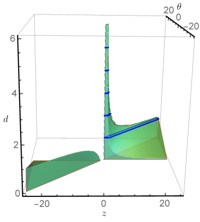
Figure 1: The parametric volume $(\theta,~{}z,~{}d)$ that is sufficient to guarantee RG flows with the right $c$-function monotonicity. The meshed lines on the surface represent the values of the integer spatial dimensions $d$. Notice how drastically the increase of the dimension $d$ shrinks the allowed region in the parametric space that gives a well behaved RG flow. The necessary conditions of section 7 are more tolerant.

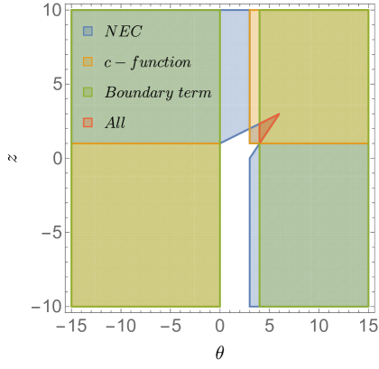
Figure 2: The window of parameters that lead always to well behaved RG flows for $d=3$ space-time dimensions. The different coloring represents where the different conditions are satisfied and the triangle is the common region in the parameter space that is sufficient to guarantee well behaved RG flow.

The sufficient $c$-function conditions for theories that exhibit anisotropic Lifshitz scaling and hyperscaling violation are more involved. These symmetries are described by the following metric

$$ds^{2}=-{\left({\frac{\theta r}{d}}\right)}^{2{\left({1-\frac{zd}{\theta}}\right)}}{\left({-dt^{2}+dx^{2}}\right)}+{\left({\frac{\theta r}{d}}\right)}^{2{\left({1-\frac{d}{\theta}}\right)}}dy^{2}+dr^{2}~{}.$$ (6.10)

The NEC (3.5) give

$${\left({z-1}\right)}{\left({d_{2}-\theta+z{\left({1+d_{1}}\right)}}\right)}\geq 0~{},\qquad\theta{\left({\theta-zd}\right)}+d_{2}d{\left({z-1}\right)}\geq 0~{},$$ (6.11)

while the monotonicity condition (4.3) gives

$$1-\frac{d_{2}+d_{1}z}{\theta}\geq 0,$$ (6.12)

and the monotonicity conditions (4.4) and (4.5) give the same condition

$$(\frac{z-1}{\theta})(1-\frac{d}{\theta})\geq 0.$$ (6.13)

The elimination of the boundary terms (2.25) provide extra conditions

$$1-\frac{d_{2}+z+d_{1}z}{\theta}\geq 0~{},\qquad 1-\frac{1+d_{2}+d_{1}z}{\theta}\geq 0~{}.$$ (6.14)

We have confirmed that the conditions (6.11), (6.12), (6.13) and (6.14) are compatible with each other and they can be satisfied simultaneously, for a small region in the parametric space, as shown in figures 2 and 2.

As seen from the form (6.10) of the metric, the isotropic limit is obtained by setting $d_{1}=0$ and $d_{2}=d$. Indeed by doing so and ignoring all the conditions derived corresponding to the $x_{i}$ dimensions, the conditions (6.11), (6.12, 6.13) and the second condition in (6.14) become (6.7), (6.8), (6.9) respectively for the Lifshitz metric.

We note that our analysis can be applied to the vacuum anisotropic hyperscaling violation theory which has the same background form (6.6), derived by a generalized Einstein-Axion-Dilaton action [27] with a potential proportional to the exponential of the dilaton [28]. It can be checked easily that this background satisfies our stated sufficient conditions and hence its RG flows satisfy the $c$-theorem.

7 Necessary Conditions on Anisotropic RG flows

So far we have considered the sufficient conditions for monotonic RG flows. In this section by performing explicitly the integrations of (2.23) and (2.24), we confirm that the necessary conditions are indeed much more relaxed. The $c$-function integral can be written as

$$\frac{4G_{N}^{(d+2)}}{\beta_{x}}\frac{\partial c_{x}}{\partial r_{m}}=e^{k_{m}}l_{x}^{d_{x}-1}d_{x}{\left[{k_{m}^{\prime}\int_{r_{m}}^{\infty}dr\frac{e^{k_{m}-A_{1}(r)}}{k^{\prime}(r)^{2}\sqrt{e^{2k(r)}-e^{2km}}}{\left({\frac{k^{\prime}(r)^{2}}{d_{x}}-A_{1}^{\prime}(r)k^{\prime}(r)-k^{\prime\prime}(r)}\right)}}\right]}$$ (7.1)

and a similar expression exists for the $c_{y}$ according to (2.24).

In the previous section, we have checked that for the Lifshitz space (6.1) to give rise to a monotonic RG-flow, the sufficient condition allows only the case of $z=1$. However, since the Lifshitz space has a scaling symmetry, one can expect the dual field theory to have a conformal symmetry and so the $c$-function should not run at all. Indeed we have checked analytically that the integrand of (7.1) vanishes identically for any value of $z$. Therefore as long as the background is allowed by the NEC, i.e. $z\geq 1$, the dual theory has constant $c$-functions and satisfy the $c$-theorem.

For the same reason one can expect that the same holds for the Lifshitz-like anisotropic spaces (6.2). We have checked this analytically and again the integrand cancel out completely for any value of $z$. It is satisfying to see that this cancellation takes place only because of our choice of $d_{x}$ and $d_{y}$ in the definition of the $c$-function. As an example, the field theories with space-dependent $\theta$-term coupling, which have a Lifshitz-like anisotropic symmetry with $z=3/2$ [26] will satisfy the $c$-theorem for our choice of the $c$-functions.

For general background with more complicated metric, the analytic method cannot be applied and one has to resort to numerical method integrating the equation (7.1). Generically the analysis is complicated and the sufficient condition obtained from the study conducted in this work could provide valuable insights on what region in the parameters space one should start focusing on.

8 Discussion

Motivated by the relevant construction in two-dimensional quantum field theories [9, 10], we have constructed an extension of the $c$-function (2.4) for higher dimensional anisotropic theories. Our proposal suggests the presence of as many independent $c$-functions as the number of independent isotropic factors within the anisotropic geometry; and that they would become at the IR fixed point, the central charges of the underlying (an)isotropic theories. Our proposed $c$-function relies on the knowledge of the entanglement entropy of a strip-shaped region and the relative scaling between the spatial directions at the fixed points. It has no UV divergences, although the entanglement entropy is divergent itself. When the full rotational symmetry is restored, our $c$-functions converge and reduce to the original proposal [12, 13] of the $c$-function for the isotropic case.

With the use of the null energy conditions, the sufficient conditions ensuring a decreasing $c$-function towards the IR take the form (4.3)-(4.5). These conditions can be expressed in terms of monotonic functions as (4.6)-(4.8). In the case the anisotropic flow admit isotropic UV fixed points, these conditions reduce to (4.9). We point out that the null energy conditions in general do not guarantee a well behaved anisotropic RG flow, in contrary to what happens in conformal theories.

We have also derived the necessary conditions for the right monotonicity of the $c$-function. They are expressed in terms of integrals of the metric fields and can be applied in a straightforward way to known gravity dual theories. For example, anisotropic RG flows with AdS UV asymptotics were recently constructed to study of the effect the confinement/deconfinemt phase transitions and the inverse anisotropic catalysis effect [27]. A numerical analysis of (7.1), could be applied to such vacuum gravity solutions to examine if there is a need to constrain further the parametric space in those theories. Other theories with anisotropic flows that our analysis can be applied include [29, 30, 31, 32].

It should be interesting to study the behavior of the $c$-functions defined here at the quantum and topological anisotropic phase transitions. The entanglement entropy is an order parameter for such phase transitions and therefore the $c$-function itself is expected to show certain signals of discontinuity at the critical region. Moreover, it would be very interesting to provide further evidence on our proposal by looking at the properties of the $c$-function in the weakly coupled anisotropic theories. The possibility that linear combinations of $c_{x}$ and $c_{y}$ may form a candidate for a holographic $c$-function cannot be excluded. In fact for theories with isotropic UV asymptotics the sum of the $c$-functions produce a invariant integral under interchanges $x\leftrightarrow y$, while for anisotropic UV dynamics the combination needs to be more involved.

We would also like to comment on further alternative applications of our work. In 3-dimensional isotropic CFTs, it has been shown that the free energy of the theory on the $S^{3}$ coincides with the entanglement entropy of a spherical surface, and therefore it can be expressed via the entropic formulation of the c-function [33, 34]. Generalization to more dimensions has also been found [35, 36]. It would be interesting to extend the $F$-theorem for anisotropic flows using the findings of our work. Moreover, our study can be reformulated with the renormalized entanglement entropy (REE) [15], where all the potential divergent terms along the RG flow have been removed and in certain cases can play the role of the $F$-function. Furthermore, the technical methods developed in our work may be applied to other non-local observables, like the heavy quark observables. As long as the observables are expressed holographically in terms of the metric fields for general holographic backgrounds (i.e. as in [37]), our methods can be applied to study their flow behavior along the RG trajectory.

Appendix A An Alternative Form for the Sufficient Conditions of Monotonicity

A set of more restricting sufficient conditions of monotonicity are derived by eliminating the second derivatives of (2.23) and (2.24) using the null energy conditions to obtain

$$\frac{\partial c_{x}}{\partial r_{m}}=\frac{\beta_{x}e^{k_{m}}l_{x}^{d_{x}-1}d_{x}}{4G_{N}^{(d+2)}}k_{m}^{\prime}\int_{0}^{l}dx\frac{1}{k^{\prime}(r)^{2}}{\left({P_{+x}-{\left({B^{\prime}(r)+A_{1}^{\prime}(r)}\right)}k^{\prime}(r)}\right)}~{},$$ (A.1)

$$\frac{\partial c_{y}}{\partial r_{m}}=\frac{\beta_{y}e^{k_{m}}l_{y}^{d_{y}-1}d_{y}}{4G_{N}^{(d+2)}}k_{m}^{\prime}\int_{0}^{l}dy\frac{1}{k^{\prime}(r)^{2}}{\left({P_{+y}-{\left({B^{\prime}(r)+A_{2}^{\prime}(r)}\right)}k^{\prime}(r)}\right)}~{},$$ (A.2)

$$P_{+x}:=\frac{1}{d_{x}}k^{\prime}(r)^{2}+d_{1}A_{1}^{\prime}(r)^{2}+d_{2}A_{2}^{\prime}(r)^{2}+N_{3}\geq 0~{}.$$ (A.3)

The conditions below are sufficient to guarantee monotonicity

$$k^{\prime}(r)\geq 0~{}\quad\mbox{and}\quad B^{\prime}(r)+A_{1}^{\prime}(r)\leq 0~{}\quad\mbox{and}\quad B^{\prime}(r)+A_{2}^{\prime}(r)\leq 0~{}.$$ (A.4)

We remark that the conditions (A.4) are sufficient to ensure a well behaved monotonic flow and take simpler form compared to (4.3)-(4.5). However, by gaining on simplicity for the sufficient conditions, they become more restrictive.

Let us note that in the case of AdS UV asymptotics, the expression of $P_{+x}$ simplifies to

$$P_{+x}=-f_{b}^{\prime}(r)e^{k(r)/{\left({d_{1}+d_{2}}\right)}+B(r)}~{},$$ (A.5)

where

$$f_{b}(r):=k^{\prime}(r)e^{-k(r)/{\left({d_{1}+d_{2}}\right)}-B(r)}~{}.$$ (A.6)

The NEC (3.7) can be expressed in terms of $f_{b}$ as

$$f_{b}^{\prime}(r)e^{k(r)/{\left({d_{1}+d_{2}}\right)}+B(r)}+\frac{2d_{1}^{2}A_{1}^{\prime}(r)^{2}+2d_{2}^{2}A_{2}^{\prime}(r)+d_{1}d_{2}{\left({A_{1}^{\prime}(r)+A_{2}^{\prime}(r)}\right)}^{2}}{d_{1}+d_{2}}\leq 0~{},$$ (A.7)

which implies that $f_{b}$ is a monotonically decreasing function. Therefore, an analysis along the lines of the section 5 can be repeated here, which would lead to stricter UV boundary conditions that ensure the $c$-function monotonicity.

References

- [1] A. B. Zamolodchikov, Irreversibility of the Flux of the Renormalization Group in a 2D Field Theory, JETP Lett. 43 (1986) 730–732.
- [2] J. L. Cardy, Is There a c Theorem in Four-Dimensions?, Phys. Lett. B215 (1988) 749–752.
- [3] Z. Komargodski and A. Schwimmer, On Renormalization Group Flows in Four Dimensions, JHEP 12 (2011) 099, [1107.3987].
- [4] Z. Komargodski, The Constraints of Conformal Symmetry on RG Flows, JHEP 07 (2012) 069, [1112.4538].
- [5] L. Girardello, M. Petrini, M. Porrati and A. Zaffaroni, Novel local CFT and exact results on perturbations of N=4 superYang Mills from AdS dynamics, JHEP 12 (1998) 022, [hep-th/9810126].
- [6] D. Z. Freedman, S. S. Gubser, K. Pilch and N. P. Warner, Renormalization group flows from holography supersymmetry and a c theorem, Adv. Theor. Math. Phys. 3 (1999) 363–417, [hep-th/9904017].
- [7] R. C. Myers and A. Sinha, Holographic c-theorems in arbitrary dimensions, JHEP 01 (2011) 125, [1011.5819].
- [8] R. C. Myers and A. Sinha, Seeing a c-theorem with holography, Phys. Rev. D82 (2010) 046006, [1006.1263].
- [9] H. Casini and M. Huerta, A Finite entanglement entropy and the c-theorem, Phys. Lett. B600 (2004) 142–150, [hep-th/0405111].
- [10] H. Casini and M. Huerta, A c-theorem for the entanglement entropy, J. Phys. A40 (2007) 7031–7036, [cond-mat/0610375].
- [11] S. Ryu and T. Takayanagi, Holographic derivation of entanglement entropy from AdS/CFT, Phys. Rev. Lett. 96 (2006) 181602, [hep-th/0603001].
- [12] S. Ryu and T. Takayanagi, Aspects of Holographic Entanglement Entropy, JHEP 08 (2006) 045, [hep-th/0605073].
- [13] R. C. Myers and A. Singh, Comments on Holographic Entanglement Entropy and RG Flows, JHEP 04 (2012) 122, [1202.2068].
- [14] T. Albash and C. V. Johnson, Holographic Entanglement Entropy and Renormalization Group Flow, JHEP 02 (2012) 095, [1110.1074].
- [15] H. Liu and M. Mezei, A Refinement of entanglement entropy and the number of degrees of freedom, JHEP 04 (2013) 162, [1202.2070].
- [16] C. Park, D. Ro and J. Hun Lee, c-theorem of the entanglement entropy, JHEP 11 (2018) 165, [1806.09072].
- [17] K. S. Kolekar and K. Narayan, On AdS2 holography from redux, renormalization group flows and c-functions, JHEP 02 (2019) 039, [1810.12528].
- [18] B. Swingle, Entanglement does not generally decrease under renormalization, J. Stat. Mech. 1410 (2014) P10041, [1307.8117].
- [19] S. Cremonini and X. Dong, Constraints on renormalization group flows from holographic entanglement entropy, Phys. Rev. D89 (2014) 065041, [1311.3307].
- [20] J. L. Cardy, Anisotropic corrections to correlation functions in finite-size systems, Nuclear Physics B 290 (1987) 355 – 362.
- [21] P. K. Kovtun and A. O. Starinets, Quasinormal modes and holography, Phys. Rev. D72 (2005) 086009, [hep-th/0506184].
- [22] R. M. Wald, General relativity. Chicago Univ. Press, Chicago, IL, 1984.
- [23] R. V. Buniy, S. D. H. Hsu and B. M. Murray, The Null energy condition and instability, Phys. Rev. D74 (2006) 063518, [hep-th/0606091].
- [24] S. Dubovsky, T. Gregoire, A. Nicolis and R. Rattazzi, Null energy condition and superluminal propagation, JHEP 03 (2006) 025, [hep-th/0512260].
- [25] C. Hoyos and P. Koroteev, On the Null Energy Condition and Causality in Lifshitz Holography, Phys. Rev. D82 (2010) 084002, [1007.1428].
- [26] T. Azeyanagi, W. Li and T. Takayanagi, On String Theory Duals of Lifshitz-like Fixed Points, JHEP 0906 (2009) 084, [0905.0688].
- [27] D. Giataganas, U. Gürsoy and J. F. Pedraza, Strongly-coupled anisotropic gauge theories and holography, Phys. Rev. Lett. 121 (2018) 121601, [1708.05691].
- [28] D. Giataganas, D.-S. Lee and C.-P. Yeh, Vacuum solution of section 7.1.2, Quantum Fluctuation and Dissipation in Holographic Theories: A Unifying Study Scheme, JHEP 08 (2018) 110, [1802.04983].
- [29] S. Jain, R. Samanta and S. P. Trivedi, The Shear Viscosity in Anisotropic Phases, JHEP 10 (2015) 028, [1506.01899].
- [30] I. Aref’eva and K. Rannu, Holographic Anisotropic Background with Confinement-Deconfinement Phase Transition, JHEP 05 (2018) 206, [1802.05652].
- [31] D. Mateos and D. Trancanelli, The anisotropic N=4 super Yang-Mills plasma and its instabilities, Phys.Rev.Lett. 107 (2011) 101601, [1105.3472].
- [32] D. Giataganas, Observables in Strongly Coupled Anisotropic Theories, PoS Corfu2012 (2013) 122, [1306.1404].
- [33] H. Casini, M. Huerta and R. C. Myers, Towards a derivation of holographic entanglement entropy, JHEP 05 (2011) 036, [1102.0440].
- [34] J. K. Ghosh, E. Kiritsis, F. Nitti and L. T. Witkowski, Holographic RG flows on curved manifolds and the -theorem, JHEP 02 (2019) 055, [1810.12318].
- [35] S. Giombi and I. R. Klebanov, Interpolating between and , JHEP 03 (2015) 117, [1409.1937].
- [36] T. Kawano, Y. Nakaguchi and T. Nishioka, Holographic Interpolation between and , JHEP 12 (2014) 161, [1410.5973].
- [37] D. Giataganas, Probing strongly coupled anisotropic plasma, JHEP 1207 (2012) 031, [1202.4436].