Matrix product state algorithms for Gaussian fermionic states

Abstract

While general quantum many-body systems require exponential resources to be simulated on a classical computer, systems of non-interacting fermions can be simulated exactly using polynomially scaling resources. Such systems may be of interest in their own right, but also occur as effective models in numerical methods for interacting systems, such as Hartree-Fock, density functional theory, and many others. Often it is desirable to solve systems of many thousand constituent particles, rendering these simulations computationally costly despite their polynomial scaling. We demonstrate how this scaling can be improved by adapting methods based on matrix product states, which have been enormously successful for low-dimensional interacting quantum systems, to the case of free fermions. Compared to the case of interacting systems, our methods achieve an exponential speedup in the entanglement entropy of the state. We demonstrate their use to solve systems of up to one million sites with an effective MPS bond dimension of $10^{15}$.

I Introduction

Non-interacting or weakly interacting fermions play a crucial role in many aspects of condensed matter theory and quantum chemistry. For example, using density functional theory, many materials can be accurately approximated by weakly interacting fermions; Hartree-Fock theory is an excellent starting point for quantum chemical calculations; and transport in electronic nanodevices is often captured by non-interacting models. While the computational effort in all these applications scales polynomially with the size of the system that must be considered, the desire to obtain a realistic description – reached, for example, by including many orbitals in a complex material or a microscopic multi-band model for a nanostructure – means that computing properties of a non-interacting fermion model can nevertheless become a computational bottleneck.

For interacting quantum systems, tensor networks have in many cases become the tool of choice for numerical simulations. They exploit the locality of entanglement in the low-energy states of local quantum Hamiltonians for a more compact classical description of these states. The prototypical example are matrix-product states [1; 2], which form the basis of the density matrix renormalization group (DMRG) [3; 4]. Since its inception, DMRG has become the standard method to solve one-dimensional quantum systems [5; 6]. Many extensions of matrix-product states to higher-dimensional systems have been suggested [7; 8; 9; 10; 11; 12; 13; 14]; for recent reviews, see Refs. 15; 16; 17.

In this paper, we will show that it is possible to apply the benefits of tensor networks to non-interacting fermions to obtain significantly more efficient numerical methods for the simulation of very large free fermion systems, allowing us to simulate systems far beyond what is possible with existing methods. While tensor network states have previously been described for systems of free fermions [18; 19; 20; 21; 22; 23; 24], thus far they have not been used primarily as numerical tools. In this work, we will describe practical tensor network algorithms to compute the many-body ground state as well as the dynamics of many-body states for free-fermion systems. Our methods capture the full equal-time Green’s function of the system, from which any physical observable can be computed. While exact methods for this property scale cubically with the system size, our approach scales linearly with the length of a quasi-one-dimensional system and thus outperforms exact methods significantly.

We work within the framework of Gaussian fermionic matrix product states (GFMPS) [19]. These states are constructed using Gaussian fermionic states, which are the most general class of states for which a Wick’s theorem holds, i.e. whose equal-time correlation functions are characterized fully through the equal-time single-particle Green’s function. We will review this formalism in Sec. II, where we also introduce the required building blocks for Gaussian tensor network algorithms, such as contraction and decomposition of tensors. We introduce the specific case of GFMPS in Sec. III, where we also discuss the key technical tool of our work: a canonical form for GFMPS. This crucial technical step will allow us to generalize many well-established numerical algorithms for matrix-product states, such as single- and two-site DMRG as well as time evolution approaches such as TDVP [25; 26] to the Gaussian setting; this will be discussed in Secs. IV and V. Finally, in Sec. VI, we numerically demonstrate the performance of our algorithms.

I.1 Quadratic fermion systems

To set the stage, consider a lattice system of $N$ sites, each comprised of some number $n_{s}$ of fermionic modes. For our purposes, it will be convenient to work in a basis of self-adjoint – so-called Majorana – fermions $c_{i}$, with $c_{i}^{\dagger}=c_{i}$ and $\{c_{i},c_{j}\}=2\delta_{ij}$. A fermionic system comprised of conventional complex fermions created by some operator $a_{i}^{\dagger}$ can always be rewritten in such a Majorana basis by taking $c_{2i-1}=a_{i}+a_{i}^{\dagger}$, $c_{2i}=-i(a_{i}-a_{i}^{\dagger})$. We will be interested in quadratic Hamiltonian, i.e., Hamiltonians of the form

$$\mathcal{H}=-i\sum_{ij}H_{ij}c_{i}c_{j}+E\ ,$$ (1)

with $E$ a constant offset. We denote the total number of Majorana modes, which must be even in a physical system, by $M=2\sum n_{s}$. Thus, $H$ is a real matrix of size $M\times M$, which we can choose w.l.o.g. anti-symmetric, $H^{\intercal}=-H$, and we will do so in the following.

To compute properties of such a system, one can fully diagonalize the matrix $H$ to obtain all single-particle eigenvalues and eigenvectors, from which all other observables can be constructed. In the absence of any special structure of $H$, this will scale as $\mathcal{O}(N^{3})$. If, on the other hand, only a few low-lying single-particle eigenstates (or a few states near a particular energy, such as the Fermi energy) are desired and the matrix $A$ is sufficiently sparse (as is the case for short-range hopping models), one can use sparse Krylov-space diagonalization methods such as Lanczos or shift-and-invert methods. These are generally expected to scale linearly in $N$ and the number of non-zero elements per row of $A$, as well as exhibit some dependence on spectral properties such as the energy gap. However, it should be emphasized that having computed only a few low-lying states, physical observables such as the density or more generally equal-time Green’s function cannot be computed.

There are many other methods that overcome this limitation. A very efficient method to compute the spectral density of some operator (as well as certain dynamical correlation functions) in a time that scales only linearly with the number of modes is the kernel polynomial method (KPM) [27]. There is also a large variety of Green’s-function-based methods. To compute the frequency-dependent Green’s function, the recursive Green’s function (RGF) approach [28; 29] can be used. For a one-dimensional system, this method scales linearly with the length; for two- or three-dimensional systems, the method can be applied by taking the system to be a one-dimensional collection of ”slices”. However, to obtain equal-time properties, a frequency integral must be taken. Finally, the non-equilibrium Green’s function approach [30] incorporates systems driven out of equilibrium, for example by an applied voltage in a nanodevice. For a recent review and a related wavefunction-based approach, see Ref. 31. Finally, in the context of density functional theory, several approximate methods to solve the Kohn-Sham equation in linear time have been developed, see e.g. Ref. 32. In contrast to these methods, our GFMPS method is based on the many-body wavefunction for a low-energy or time-dependent state of the system, and thus allows the straightforward calculation of arbitrary expectation values without having to integrate over frequencies. Furthermore, our approach gives access to quantities such as the entanglement spectrum and entanglement entropy of the state.

I.2 Gaussian tensor networks

The power of matrix-product states is most easily understood from the properties of the Schmidt decomposition. For a quantum state $|\psi\rangle$ on a tensor product space $\mathcal{H}_{A}\otimes\mathcal{H}_{B}$, it is given by

$$|\psi\rangle=\sum_{\alpha=1}^{M}s_{\alpha}|A_{\alpha}\rangle|B_{\alpha}\rangle,$$ (2)

where $s_{\alpha}\geq 0$ are real, and the Schmidt vectors $|A_{\alpha}\rangle$, $|B_{\alpha}\rangle$ are orthonormal bases for $\mathcal{H}_{A}$ and $\mathcal{H}_{B}$, respectively. The von Neumann entanglement entropy between $A$ and $B$ is given by $S=-\operatorname{Tr}(\rho_{A}\log\rho_{A})=-\sum s_{\alpha}^{2}\log s_{\alpha}^{2}$, and is bounded by $S\leq\log(M)$. Thus, coarsely speaking, the number of terms that are relevant grows exponentially with the bipartite entanglement of the state.

Given that low-energy states of local Hamiltonians are weakly entangled in the sense that they exhibit area law scaling of the entanglement entropy [33; 34; 35; 36], one can exploit the properties of the Schmidt decomposition to construct more compact representations of such states. In particular, it is natural to assume that the Schmidt values $s_{\alpha}$ decay very quickly with $\alpha$ in such weakly entangled states [37; 38; 39; 40; 34; 35; 36]. This directly leads to the construction of matrix-product states, which can be obtained by recursively performing a Schmidt decomposition between all sites of a one-dimensional system and truncating the sum on each bond to the $D$ largest Schmidt values $s_{\alpha}$. The computational cost of such a state will scale exponentially with the bipartite entanglement entropy.

In systems of non-interacting fermions, the Schmidt decomposition and thus also the bipartite entanglement take a simpler form. This is due to the fact that reduced density matrix for a subsystem is itself a Gibbs state of a quadratic Hamiltonian [41; 42; 43; 44]. Thus, even its many-body spectrum can be obtained through single-particle modes and their eigenvalues, and the entanglement can be fully characterized through mode-wise entanglement [41; 44] between single-particle modes in each part of the bipartite system. In other words, the Schmidt decomposition of a Gaussian state can itself be expressed entirely in terms of Gaussian states. Crucially, each mode can contribute a fixed amount to the bipartite entanglement, and the maximum entanglement is thus linear in the number of modes rather than logarithmic in the number of terms in the Schmidt decomposition. This constitutes an exponential compression of the Schmidt decomposition in the Gaussian case.

To exploit this computationally, one can construct a Gaussian MPS (GFMPS) in an analogous fashion to the interacting case by recursively applying the Schmidt decomposition on each bond of a given Gaussian state. Owing to the structure of Gaussian states, such a GFMPS will scale only polynomially rather than exponentially with the amount of bipartite entanglement.

This exponential speedup also benefits more general tensor networks. In the context of a conventional tensor network, a tensor is nothing but a high-dimensional array of numbers, which are enumerated by an array of indices. The number of indices is commonly referred to as “tensor rank” $R$ (not to be confused with the matrix rank), and each index runs over integers $1,\ldots,D$, where $D$ is referred to as the bond dimension. A quantum state is expressed through such a tensor network by identifying some indices of the tensors with physical degrees of freedom, and contracting (summing) over the remaining ones in some predetermined pattern.

To understand the case of a Gaussian tensor network, it is convenient to think of a rank-$R$ tensor of bond dimension $D$ as a quantum state on the tensor product of $R$ $D$-dimensional Hilbert spaces. One can now consider the case where this state is Gaussian, i.e. it satisfies a Wick theorem and can thus be described completely through the expectation values of quadratic operators. Such a representation is exponentially more compact, i.e. requires only $\mathcal{O}(R\log D)$ rather than $\mathcal{O}(D^{R})$ numbers. Using techniques that we will discuss in more detail below, one can generalize the contraction of tensors and other important operations on tensor networks to this framework.

II Covariance matrix formalism for Gaussian tensor networks

We will now introduce Gaussian tensor networks on a more technical level. This will establish the essential tools that we will use for the construction of Gaussian MPS in Sec. III as well as specific optimization algorithms in Sec. IV. We first review the fermionic covariance matrix formalism. We follow the conventions of Ref. 45; for further details, see also Ref. 46. Throughout this section, we will assume a system of $2n$ Majorana fermions described by a Hamiltonian of the form (1).

II.1 Covariance matrix formalism

Gaussian states are states that are fully characterized through their equal-time two-point correlation functions. A convenient formalism for describing these is the covariance matrix, which is given by

$$\gamma_{ij}=\tfrac{\mathrm{i}}{2}\mathrm{tr}\big{(}\rho[c_{i},c_{j}]\big{)}\ .$$ (3)

The covariance matrix $\gamma$ is real and antisymmetric, and satisfies $\gamma^{2}\geq-\openone$; for pure states,

$$\gamma^{2}=-\openone\ .$$ (4)

In the following, we discuss some further properties of quadratic Hamiltonians and Gaussian states.

Energy of a state and normal form.

The energy of a state $\rho$ under the Hamiltonian $\mathcal{H}$ [Eq. (1)] is

$$\mathrm{tr}[\mathcal{H}\rho] =-\sum H_{ij}\>\mathrm{i}\>\mathrm{tr}(\rho c_{i}c_{j})+E$$ (5)

$$=-\sum H_{ij}\gamma_{ij}+E$$

$$=\mathrm{tr}(H\gamma)+E\ .$$

Any real antisymmetric matrix $A$ (such as $H$ or $\gamma$) can be brought into a canonical form by an orthogonal transformation,

$$OAO^{\intercal}=\bigoplus_{k=1}^{n}\begin{pmatrix}&\lambda_{k}\\ -\lambda_{k}\end{pmatrix}\ ,$$ (6)

with $\lambda_{k}\geq 0$. If $A$ is of odd size, additionally a single $0$ block appears. Note that $\pm\lambda_{k}$ are exactly the eigenvalues of the Hermitian matrix $iA$.

We can use this to bring a Hamiltonian of the form Eq. (1) into a normal form

$$\mathcal{H}=-\frac{\mathrm{i}}{2}\>\sum_{k=1}^{n}\epsilon_{k}[\eta_{2k-1},\eta_{2k}]\ ,$$ (7)

where $\eta_{k}$ are new canonical Majorana operators given by $\eta_{k}=\sum_{i}O_{ki}c_{i}$, with $OHO^{\intercal}=\bigoplus_{k=1}^{n}\big{(}\begin{smallmatrix}&\epsilon_{k}/2\\ -\epsilon_{k}/2\end{smallmatrix}\big{)}$. The $\epsilon_{k}$ correspond exactly to the non-negative half of the single-particle eigenvalues of the equivalent Bogoliubov-de Gennes Hamiltonian. The ground state of $\mathcal{H}$, which we will denote as $|0\rangle$, is characterized by having $\mathrm{i}\eta_{2k-1}\eta_{2k}|0\rangle=|0\rangle$ for all $k=1,\ldots,n$, and thus has total energy $E_{0}=-\sum\epsilon_{k}$. Its covariance matrix in the basis of canonical operators $\eta_{k}$ is thus given by

$$\tilde{\gamma}_{0}=\tfrac{i}{2}\langle 0|[\eta_{i},\eta_{j}]|0\rangle=\bigoplus\begin{pmatrix}&1\\ -1\end{pmatrix}\ .$$ (8)

Using the orthogonal matrix $O$ that brings $A$ into the normal form, we can obtain the covariance matrix in the basis of local, physical Majorana operators $c_{i}$ as $\gamma_{0}=O^{\intercal}\tilde{\gamma}_{0}O$. Using Eq. (5), we can verify that the ground state energy is indeed $E_{0}=-\sum\epsilon_{k}$. Numerically, $\gamma_{0}$ can be determined by diagonalizing the antisymmetric matrix $H$ (giving imaginary eigenvalues) and then replacing them by the sign of the imaginary part. For other approaches, see Ref. 47.

Expectation values and state overlaps.

The expectation value of arbitrary operators in a Gaussian state can be computed using Wick’s theorem, which takes a particularly simple form in the representation of Gaussian covariance matrices. Consider a product of Majorana operators $C=\prod_{i\in\mathcal{I}}c_{i}$. The expectation value of $C$ in a state $|\phi\rangle$ with CM $\gamma$ is given by [45]

$$\langle\phi|C|\phi\rangle=\operatorname{Pf}(i\gamma_{\mathcal{I}}),$$ (9)

where $\gamma_{\mathcal{I}}$ is the submatrix of $M$ with row and column indices in $\mathcal{I}$.

The square modulus of the overlap between two states is easily determined from the covariance formalism [48; 45]. Consider two many-body states $|A\rangle$ and $|B\rangle$ with corresponding covariance matrices $\gamma_{A}$ and $\gamma_{B}$ and the same fermion parity, i.e. $\operatorname{Pf}(i\gamma_{A})=\operatorname{Pf}(i\gamma_{B})=p$. Then,

$$|\langle A|B\rangle|^{2}=p2^{-n}\operatorname{Pf}(\gamma_{A}+\gamma_{B}).$$ (10)

When the phase of the overlap is also desired, a complication arises from the fact that the covariance matrix formalism does not capture the global phase of the state – clearly for some fermionic state $|\psi\rangle$, all states $e^{i\phi}|\psi\rangle$ will have the same expectation values of physical operators, and thus the same covariance matrix. To overcome this problem, one can introduce a reference state $|C\rangle$ and observe that $\langle C|A\rangle\langle A|B\rangle\langle B|C\rangle$ is invariant under multiplying any of the three states by a phase. Therefore, it can be computed from the covariance formalism; for explicit expressions, see Ref. 45.

Composite systems.

Consider a Gaussian state described by a covariance matrix $\gamma^{\prime}$ on $N$ modes, and $\gamma^{\prime\prime}$ on $M$ modes. The joint state $\gamma$ is characterized by the direct sum of the covariance matrices,

$$\gamma=\gamma^{\prime}\oplus\gamma^{\prime\prime}=\left(\begin{matrix}\gamma^{\prime}&0\\ 0&\gamma^{\prime\prime}\end{matrix}\right).$$ (11)

To describe a general state of such a joint system, it is convenient to introduce collective labels for the Majorana modes in each subsystem. For example, we can denote the $N$ modes of the state $\gamma^{\prime}$ as $a$, and the $M$ modes of the other system as $b$. A general Gaussian state of the joint system thus takes the block form

$$\gamma=\left(\begin{matrix}\gamma_{aa}&\gamma_{ab}\\ -\gamma_{ab}^{\intercal}&\gamma_{bb}\end{matrix}\right).$$ (12)

where $\gamma_{aa}$ contains the correlations of the $a$ modes, $\gamma_{ab}$ the correlations of $a$ modes with $b$ modes, etc. We will occasionally write $|a|$ for the number of modes in $a$, i.e. $|a|=N$. More generally, for multipartite systems, such as a tripartite system with modes $a$, $b$, and $c$, we can express $\gamma$ in different partitions, e.g.

$$\gamma=\begin{pmatrix}\gamma_{aa}&\gamma_{ab}&\gamma_{ac}\\ \gamma_{ba}&\gamma_{bb}&\gamma_{bc}\\ \gamma_{ca}&\gamma_{cb}&\gamma_{cc}\end{pmatrix}=\begin{pmatrix}\gamma_{ab|ab}&\gamma_{ab|c}\\ \gamma_{c|ab}&\gamma_{c|c}\end{pmatrix}\ ,$$ (13)

where we use a vertical bar to separate row and column indices when ambiguous; e.g., $\gamma_{ab|c}$ holds the correlations of the modes $a$ and $b$ vs. $c$, i.e., $\gamma_{ab|c}=\left(\begin{smallmatrix}\gamma_{ac}\\ \gamma_{bc}\end{smallmatrix}\right)$. We will generally follow this notation throughout this paper. Note that due to the explicit labeling of the modes in this notation, the actual ordering of the blocks in the matrix does not matter.

Partial traces.

The dual operation to composing systems is the partial trace, i.e. considering only the state of a subsystem; we will make frequent use of it in this paper. Given a system composed of $N+M$ modes $a$ and $b$ with covariance matrix

$$\gamma=\left(\begin{matrix}\gamma_{aa}&\gamma_{ab}\\ -\gamma_{ab}^{\intercal}&\gamma_{bb}\end{matrix}\right)\ ,$$ (14)

the covariance matrix which describes the state of the $a$ modes (i.e., the system after tracing out the $b$ modes) is given by $\gamma_{aa}$; this follows immediately from the definition of the covariance matrix.

II.2 Tensor networks and contraction

Formalism.

Tensor networks are a way to describe multipartite quantum states

$$|\Psi\rangle=\sum_{i_{1},\dots,i_{N}}c_{i_{1},\dots,i_{N}}|i_{1},\dots,i_{N}\rangle$$ (15)

by rewriting $c_{i_{1},\dots,i_{N}}=\sum_{\alpha_{k}}\prod C_{\{i_{s},\alpha_{p}\}}$, using tensors $C_{\{i_{s}\},\{\alpha_{p}\}}$ which depend on only on a few (if any) physical indices $\{i_{s}\}$ and auxiliary indices (or entanglement degrees of freedom) $\{\alpha_{p}\}$ each, where each auxiliary index is contained in exactly two tensors, and where the auxiliary indices are contracted (i.e. summed over). In the context of fermionic tensor networks, it is convenient to instead consider each $C_{\{i_{s}\},\{\alpha_{p}\}}$ as describing a pure state (“fiducial state”) $|C_{\{i_{s}\},\{\alpha_{p}\}}\rangle=\sum C_{\{i_{s}\},\{\alpha_{p}\}}|\{i_{s}\},\{\alpha_{p}\}\rangle$ of the physical and virtual indices jointly, where the contraction is achieved by projecting pairs of virtual indices onto a maximally entangled state $|\omega_{\alpha,\alpha^{\prime}}\rangle$:

$$|\Psi\rangle=\left(\bigotimes\langle\omega_{\alpha,\alpha^{\prime}}|\right)\left(\bigotimes|C_{\{i_{s}\},\{\alpha_{p}\}}\rangle\right)\ .$$ (16)

This framework is particularly suited for the case of fermionic tensor network states, as it removes the requirement to specify an ordering of the fermionic tensors (and bonds), since both $\langle\omega_{\alpha,\alpha^{\prime}}|$ and $|C_{\{i_{s}\},\{\alpha_{p}\}}\rangle$ have fixed fermion parity, and all tensors $C$ mutually commute (as they don’t share fermionic operators), and similarly all bonds $\omega$.

Figure 1: (a) Tensors are described by their covariance matrix $\gamma$, which has blocks of rows/columns labeled by the different indices; the size of each block equals the number of Majorana modes in the block. (b) Since $\gamma$ describes pure and mixed state on equal footing, we will sometimes draw even pure state tensors with both ket and bra indices. (c) This allows e.g. to naturally capture tracing of an index in the graphical calculus.

Contraction.

In the case of Gaussian fermionic tensor networks, the fiducial states are given by covariance matrices $\gamma$ which are indexed by the corresponding physical and auxiliary modes. The maximally entangled state $|\omega\rangle$ (which can either be a product of maximally entangled states between complex fermions, or a product of pairs of Majorana fermions in their joint vacuum) is itself Gaussian, such that each contraction gives rise to a new Gaussian state. The basic step is thus the contraction of two Gaussian tensors (i.e. states). This corresponds to integrating out the auxiliary degrees of freedom in a Gaussian integral, and thus gives rise to a Schur complement [49; 50; 51; 46].

This leads to the following explicit expressions for contraction: Given two tensors

$$G=\left(\begin{matrix}G_{aa}&G_{ac}\\ -G_{ac}^{\intercal}&G_{cc}\end{matrix}\right)\quad\mbox{and}\quad H=\left(\begin{matrix}H_{bb}&H_{bc^{\prime}}\\ -H_{bc^{\prime}}^{\intercal}&H_{c^{\prime}c^{\prime}}\end{matrix}\right),$$ (17)

(possibly with blocked indices), the tensor resulting from contracting the $c$ index of $G$ with the $c^{\prime}$ index of $H$ is given by

$$K=\left(\begin{matrix}K_{aa}&K_{ab}\\ -K_{ab}^{\intercal}&K_{bb}\end{matrix}\right)= \left(\begin{matrix}\!G_{aa}\\ &\!\!H_{bb}\end{matrix}\right)\!$$ (18)

$$+\!\left(\begin{matrix}G_{ac}\\ &\!\!H_{bc^{\prime}}\end{matrix}\right)\! \left(\begin{matrix}\!G_{cc}&\openone\\ -\openone&H_{c^{\prime}c^{\prime}}\end{matrix}\right)^{\!\!-1\!}\!\left(\begin{matrix}\!G_{ac}\\ &\!\!H_{bc^{\prime}}\!\end{matrix}\right)^{\!\intercal}\ .$$

Note that the contraction is oriented (swapping $c$ and $c^{\prime}$ changes the sign of the $\openone$’s); we will from now on use the notation $c\triangleright c^{\prime}$ to indicate the order. The matrix inverse in Eq. (18) can be carried out block-wise using Schur complements. Explicitly,

$$\begin{pmatrix}A&\openone\\ -\openone&D\end{pmatrix}^{-1}=\\ \begin{pmatrix}(DA+\openone)^{-1}\\ &(AD+\openone)^{-1}\end{pmatrix}\begin{pmatrix}D&-\openone\\ \openone&A\end{pmatrix}$$ (19)

and as a special case which we will use later

$$\begin{pmatrix}A&\openone\\ -\openone&0\end{pmatrix}^{-1}=\begin{pmatrix}0&-\openone\\ \openone&A\end{pmatrix}\ .$$ (20)

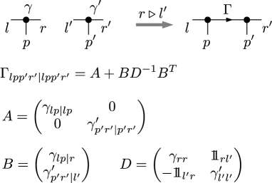
Figure 2: Contraction of two indices $r$ and $l^{\prime}$ (contraction is oriented, denoted as $r\triangleright l^{\prime}$, and indicated by the arrow on the contracted index). The CM $\Gamma$ of the resulting state is obtained as a Schur complement, as given by the formulas in the figure or Eq. (18). (Here, $\openone_{xy}$ denotes the identity matrix betweeen modes $x$ and $y$.)

For generalizations of this approach as well as the normalization of the state after contraction, see App. B.

Graphical calculus.

Tensor networks can be conveniently expressed using a graphical calculus, where each tensor is described by a box with one leg per index (where each index can contain any number of Majorana modes), Fig. 1a. Contraction of indices is indicated by connecting the corresponding legs; the orientation of the contraction will be indicated by an arrow. This is shown in Fig. 2.

Note that the covariance matrix formalism (and thus Gaussian tensor networks) does not distinguish between pure and mixed states. Yet, we will generally use the tensor notation for pure states; when referring to the density operator, we will instead draw the tensor twice, once for the “ket” and once for the “bra” system (Fig. 1b). In particular, an essential operation will be tracing out part of a tensor, which corresponds to contracting the “ket” and “bra” part of the corresponding index, and which will be drawn as in Fig. 1c.

II.3 Entanglement in Gaussian states and Schmidt decomposition

A crucial step in the DMRG algorithm is the Schmidt decomposition, i.e., the decomposition of a bipartite entangled state $|\Psi\rangle$ in the form $|\Psi\rangle=\sum_{k}\lambda_{k}|\ell_{k}\rangle|r_{k}\rangle$ with orthonormal vectors $\{|\ell_{k}\rangle\}$ and $\{|r_{k}\rangle\}$ (see also Sec. II.4.1).

The procedure for fermionic Gaussian states is quite analogous. Consider a pure bipartite Gaussian state

$$\gamma=\left(\begin{matrix}\gamma_{aa}&\gamma_{ab}\\ -\gamma_{ab}^{\intercal}&\gamma_{bb}\end{matrix}\right)\ ,$$ (21)

and assume for the moment that $\gamma_{ab}$ is square (i.e., the two systems have the same dimension) and has full rank; this corresponds to the case where all modes on either side are entangled. Since $\gamma$ is pure, we have $\gamma^{2}=-\openone$, which implies

$$\gamma_{aa}^{2}=\gamma_{ab}^{\phantom{\intercal}}\gamma_{ab}^{\intercal}-\openone\ ,\quad\gamma_{bb}^{2}=\gamma_{ab}^{\intercal}\gamma_{ab}^{\phantom{\intercal}}-\openone\ ,$$ (22)

as well as $\gamma_{aa}\gamma_{ab}=-\gamma_{ab}\gamma_{bb}$, or equivalently

$$\gamma_{bb}=-\gamma_{ab}^{-1}\gamma_{aa}\gamma_{ab}$$ (23)

We now perform an SVD of $\gamma_{ab}$, $O\gamma_{ab}Q^{\intercal}=\Lambda_{ab}$, where $\Lambda_{ab}$ is diagonal with positive entries which are ordered descendingly, and $O$ and $Q$ are real orthogonal, as they diagonalize the real symmetric matrices $\gamma_{ab}^{\phantom{\intercal}}\gamma_{ab}^{\intercal}$ and $\gamma_{ab}^{\intercal}\gamma_{ab}^{\phantom{\intercal}}$, respectively. Eq. (22) then immediately implies that also $O\gamma_{aa}^{2}O^{\intercal}$ is diagonal with descending entries. Following Eq. (6), we find that

$$O\gamma_{aa}O^{\intercal}=\bigoplus_{k}\begin{pmatrix}&\lambda_{k}\\ -\lambda_{k}\end{pmatrix}$$ (24)

(possibly after rearranging rows of $O$ within degenerate blocks; by performing the same permutation on $Q$, we can ensure that $O\gamma_{ab}Q^{\intercal}$ remains diagonal). Therefore,

$$Q\gamma_{bb}Q^{\intercal} =Q(-\gamma^{-1}_{ab}\gamma_{aa}\gamma_{ab})Q^{\intercal}$$ (25)

$$=-(O\gamma_{ab}Q^{\intercal})^{-1}(O\gamma_{aa}O^{\intercal})(O\gamma_{ab}Q^{\intercal})$$ (26)

must be again of the form

$$Q\gamma_{bb}Q^{\intercal}=\bigoplus_{k}\begin{pmatrix}&-\lambda_{k}\\ \lambda_{k}\end{pmatrix}\ ,$$ (27)

where the fact that the entries $\lambda_{k}$ equal those in Eq. (24) follow from (22), as well as that

$$O\gamma_{ab}Q^{\intercal}=\bigoplus_{k}\begin{pmatrix}\mu_{k}\\ &\mu_{k}\end{pmatrix}$$ (28)

with $\mu_{k}=\sqrt{1-\lambda_{k}^{2}}$. Together, we find that the local rotations $O\oplus Q$ transform $\gamma$ to

$$(O\oplus Q)\gamma(O\oplus Q)^{\intercal}=\bigoplus_{k}W(\lambda_{k})\ ,$$ (29)

with

$$W(\lambda_{k})=\begin{pmatrix}&\lambda_{k}&\mu_{k}\\ -\lambda_{k}&&&\mu_{k}\\ -\mu_{k}&&&-\lambda_{k}\\ &-\mu_{k}&\lambda_{k}\end{pmatrix},\ \>\mu_{k}=\sqrt{1-\lambda_{k}^{2}}\ ,$$ (30)

where each block $W(\lambda_{k})$ captures the correlations between two $a$ and two $b$ Majorana modes (in this order). This is the fermionic Gaussian equivalent of the Schmidt decomposition (and of the Williamson normal form for bosonic Gaussian states), a result first derived by Botero and Reznik [44].

From this form, the von Neumann entanglement entropy between the modes $a$ and $b$ is now easily found to be

$$S_{\mathrm{vN}}=\sum_{k}H\left(\frac{1-\lambda_{k}}{2}\right)$$ (31)

with $H(p)=-p\log p-(1-p)\log(1-p)$.

In the more general case where $\gamma_{ab}$ does not have full rank (or is not square), we can still perform an SVD of $\gamma_{ab}$, which in that case will give rise to blocks where $\gamma_{ab}\gamma_{ab}^{\intercal}$ (or $\gamma_{ab}^{\intercal}\gamma_{ab}$) is zero. Eq. (22) implies that the corresponding blocks of $\gamma_{aa}$ ($\gamma_{bb}$) decouple and are equal to $\bigoplus\left(\begin{smallmatrix}&-1\\ 1\end{smallmatrix}\right)$, i.e., they describe a mode in a pure (vaccum) state, which is thus not entangled to any other mode. In the general case, we thus obtain the form

$$(O\oplus Q)\gamma(O\oplus Q)^{\intercal}=\\ \bigg{[}\bigoplus\left(\begin{smallmatrix}&-1\\ 1\end{smallmatrix}\right)\bigg{]}\,\oplus\,\bigg{[}\bigoplus_{k}W(\lambda_{k})\bigg{]}\,\oplus\,\bigg{[}\bigoplus\left(\begin{smallmatrix}&-1\\ 1\end{smallmatrix}\right)\bigg{]},$$ (32)

where the first (last) term in the sum lives only on the $a$ ($b$) modes, and the middle term captures their correlations; as before, it is obtained from the SVD of $\gamma_{ab}$, together with a suitable rearrangement of degenerate modes.

Note that while instead of performing the SVD of $\gamma_{ab}$, we could have as well diagonalized $\gamma_{aa}$ and $\gamma_{bb}$. The approach approach chosen here has two advantages: First, it doesn’t require to match up eigenvalues, and second, the singular values of $\gamma_{ab}$ relate to the square roots of the eigenvalues of $\gamma_{aa}$, thus yielding a higher accuracy (also in the basis transformations $O$ and $Q$) for weakly entangled modes.

II.4 Tensor decompositions

Tensor decompositions, such as the singular value decomposition (SVD) and the closely related QR decomposition, are core ingredients in DMRG and other tensor network algorithms. Their main role is that they allow to decompose the state in terms of an orthonormal basis; furthermore, they are an efficient way of obtaining the Schmidt decomposition and thus information about the entanglement, including the full entanglement spectrum. We will start by introducing the Gaussian version of the SVD, and then discuss how to build different related decompositions which are potentially easier or more efficient to implement.

Figure 3: Gaussian fermionic SVD. (a) The SVD expresses a CM $\gamma$ as the contraction of three CMs $L$, $\Lambda$, and $R$, where $L$ and $R$ are isometries when contracting $a$ and $b$, respectively (i.e., $L_{a^{\prime}a^{\prime}}=0$, $R_{b^{\prime}b^{\prime}}=0$), and $\Lambda=\bigoplus W(\lambda_{k})$, Eq. (30). (b) The derivation proceeds by using the Schmidt decomposition of $\gamma=(O\oplus Q)^{\intercal}\Lambda(O\oplus Q)$, rewriting $\Lambda$ as the contraction of itself with two maximally entangled states $\omega^{L}$ and $\omega^{R}$, and applying $O$ and $Q$ to $a$ and $b$, respectively.

II.4.1 Singular value decomposition (SVD)

The SVD decomposes a matrix $M=UDV^{\dagger}$, where $U$ and $V$ are isometries ($U^{\dagger}U=\openone$, $V^{\dagger}V=\openone$), and $D$ is diagonal and full rank. It is closely related to the Schmidt decomposition, which for a state $|\Psi\rangle=\sum_{ij}M_{ij}|i\rangle|j\rangle$ is obtained from the SVD of $M$ as

$$\mathclap{|\Psi\rangle=\sum d_{k}|a_{k}\rangle|b_{k}\rangle}$$ (33)

$$d_{k}=D_{kk},\,\,|a_{k}\rangle=\sum U_{ik}|i\rangle,\,\,|b_{k}\rangle=\sum V_{jk}^{*}|j\rangle\ .$$ (34)

This can be viewed as an elementary tensor network: the state $|\Psi\rangle$ is given as the contraction of tensors $U$, $D$ and $V^{*}$, where $U$ and $V^{*}$ have one auxiliary and one physical index each, and $D$ has only auxiliary indices.

We have discussed the Gaussian version of the Schmidt decomposition in the previous section, Sec. II.3. Building on this, we will now describe how to view the Schmidt decomposition as a tensor decomposition, i.e. how to view the state as the contraction of a minimal tensor network of three tensors. Specifically, the Gaussian SVD corresponds to the decomposition of the covariance matrix $\gamma$ of a bipartite system $ab$ into the contraction of three covariance matrices $L$, $\Lambda$, and $R$, as indicated in Fig. 3a (including the labeling of the modes). Here, the isometry condition $U^{\dagger}U=\openone$ translates naturally to $L_{a^{\prime}a^{\prime}}=0$, which is the CM of the maximally mixed state $\openone$, cf. Fig. 1c, and correspondingly $R_{b^{\prime}b^{\prime}}=0$; furthermore, we require $\Lambda=\bigoplus W(\lambda_{k})$ [cf. Eq. (29)].

As a starting point, consider the covariance matrix $\gamma$ written as

$$\gamma=(O\oplus Q)^{\intercal}\Lambda(O\oplus Q)$$ (35)

with orthogonal $O$ and $Q$; note that at this point, we don’t need to make any assumption about $\Lambda$, i.e. the decomposition can be more general than Eqn. (29). We will generalize it to the case with additional local degrees of freedom as in Eq. (32) in a moment. The first step is to rewrite $\Lambda$ as a contraction of three tensors $\omega^{L}$, $\Lambda$, and $\omega^{R}$, as depicted in Fig. 3b (note the relabelling of the indices of $\Lambda\equiv\Lambda_{a^{\prime\prime}b^{\prime\prime}|a^{\prime\prime}b^{\prime\prime}}$) – this is the equivalent of contracting with the identity tensor, i.e. writing $D=\openone\cdot D\cdot\openone$. The tensors $\omega^{L,R}$ are given by

$$\omega^{L}\equiv\omega^{L}_{aa^{\prime}|aa^{\prime}}=\begin{pmatrix}0&\openone_{aa^{\prime}}\\ -\openone_{a^{\prime}a}&0\end{pmatrix}$$ (36)

and

$$\omega^{R}\equiv\hat{\omega}_{b^{\prime}b|b^{\prime}b}=\begin{pmatrix}0&\openone_{b^{\prime}b}\\ -\openone_{bb^{\prime}}&0\end{pmatrix}\ .$$ (37)

They describe maximally entangled states between $a$ and $a^{\prime}$ and $b^{\prime}$ and $b$, respectively (corresponding to the identity tensor $\openone$). It is easy to check using Eqn. (18) that contracting $a^{\prime}\triangleright a^{\prime\prime}$ returns $\Lambda$, and likewise for $b^{\prime\prime}\triangleright b^{\prime}$ .

In a second step, we now take Fig. 3b and apply $O$ and $Q$ to the $a$ and $b$ system, respectively. On the left-hand side, this yields $(O\oplus Q)\Lambda(O\oplus Q)^{\intercal}=\gamma$, while on the right-hand side, $\omega^{L}$ and $\omega^{R}$ are transformed to

$$L=(O^{\intercal}\oplus\openone)\omega^{L}(O\oplus\openone)=\begin{pmatrix}0&O^{\intercal}\\ -O&0\end{pmatrix}\ ,$$ (38)

and

$$R=(\openone\oplus Q^{\intercal})\omega^{R}(\openone\oplus Q)=\begin{pmatrix}0&Q\\ -Q^{\intercal}&0\end{pmatrix}\ ,$$ (39)

respectively. Furthermore, the contraction and the application of $O$ and $Q$ commute, as they act on different indices (and as can be also checked explicitly). We thus find that $\gamma$ can be written as the contraction of $L$, $\Lambda$, and $R$, as in Fig. 3a, with $L$ and $R$ isometries. In the case where $\Lambda$ is the Schmidt decomposition, this yields the Gaussian analogue of the SVD.

In the general case where the Schmidt decomposition contains additional unentangled local degrees of freedom, as in Eq. (32), these modes need to be attached to the $a$ and $b$ system of $\omega^{L}$ and $\omega^{R}$, respectively, before applying the transformations in Eqs. (38,39); the resulting $L$ and $R$ are still isometries, and the decomposition in Fig. 3a still holds with $\Lambda=\bigoplus W(\lambda_{k})$. Note that we can always regard a pair of decoupled modes as $W(\lambda_{k}\equiv 1)$ if we do not want to minimize the bond dimension (i.e., the dimension of $\Lambda$).

II.4.2 Truncation of bond dimension.

An important scenario, in particular in $2$-site DMRG, is to truncate the bond dimension. This corresponds to carrying out an SVD $M=UDV^{\dagger}$ of a matrix $M$, and replacing it by a matrix $M^{\prime}=(UW)(W^{\dagger}DV^{\dagger})$ with an isometry $W$ such that $WW^{\dagger}$ projects onto the $\chi$ largest singular values of $D$.

In the Gaussian scenario, given a CM $\gamma$ this amounts to carrying out the Schmidt decomposition Eq. (32), and keeping only the blocks $W(\lambda_{k})$ with the $\kappa$ smallest $\lambda_{k}$, while replacing the additional blocks with

$$W(\lambda=1)\equiv\begin{pmatrix}&1\\ -1\\ &&&-1\\ &&1\end{pmatrix}\ ,$$ (40)

i.e. decoupled modes. Those modes are henceforth counted towards the decoupled modes in Eq. (32), and the truncated SVD is obtained by applying the SVD construction, Fig. 3a, with $\Lambda$ from the truncated Schmidt decomposition.

II.4.3 Variants: QR and related decompositions.

In most applications, a full SVD is not needed. For example, to obtain the canonical form of an MPS (see below for details) one only needs to be able to rewrite a covariance matrix $\gamma\equiv\gamma_{ab|ab}$, with $|a|\geq|b|$, as the contraction of an isometry and a tensor with equal-sized systems on both sides. (In DMRG, $a$ corresponds to the left virtual + physical modes, while $b$ corresponds to the right virtual modes.) To this end, we need to isolate modes in $a$ that are not entangled with any modes in $b$; we will denote the modes that are unentangled as $a_{0}$ and the others as $a_{1}$, i.e. $|a|=|a_{0}|+|a_{1}|$ and $|a_{1}|=|b|$. (We assume that all modes in $b$ are entangled with modes in $a$, as happens in practice; the generalization is straightforward.) To achieve this, we find an $|a|\times|a|$ orthogonal transformation $O$ such that

$$(O\oplus\openone)\gamma(O\oplus\openone)^{\intercal}=\left(\begin{array}[]{c|cc}\gamma_{a_{0}a_{0}}&0&0\\ \hline\cr 0&\gamma_{a_{1}a_{1}}&X\\ 0&-X^{\intercal}&\gamma_{bb}\end{array}\right)$$ (41)

where $\gamma_{a_{0}a_{0}}=\bigoplus\left(\begin{smallmatrix}&-1\\ 1\end{smallmatrix}\right)$, and $X$ is $|b|\times|b|$. Note that this is a weaker version of the decomposition of Eqn. (29), where no transformation is applied on the $b$ modes. To obtain this form, it is sufficient to choose $O$ such that

$$O\gamma_{ab}=\begin{pmatrix}0\\ X\end{pmatrix}$$ (42)

with $X$ a square matrix; this can e.g. be achieved by determining the kernel of $\gamma_{ab}^{\intercal}$ (or the image of $\gamma_{ab}$). The fact that this implies $\gamma_{a_{0}a_{1}}=0$ can be verified by invoking purity of the state. Once such an $O$ is found, following the SVD construction of Fig. 3a with $Q=\openone$ and $\Lambda\equiv\left(\begin{smallmatrix}\gamma_{a_{1}a_{1}}&X\\ -X^{\intercal}&\gamma_{bb}\end{smallmatrix}\right)$ gives the desired result. For the case where $|a|\leq|b|$, the equivalent transformation is obtained by acting with $O$ on the $b$ modes. Note that for $|a|=|b|$, $O$ can be chosen trivial.

Similarly, in order to obtain a decomposition which allows to truncate the bond dimension (such as in 2-site DMRG), it is sufficient to determine $O$ such that $\gamma_{aa}$ is diagonalized; this allows to determine which modes decouple, and yields the $\lambda_{k}$ of the $W(\lambda_{k})$ which can be used to identify and disentangle the least entangled modes, without the need to determine $Q$.

III Gaussian fermionic MPS (GFMPS)

III.1 Construction

Figure 4: Construction of a Gaussian fermionic MPS: To each site, we associate a tensor $\gamma^{s}_{l_{s}p_{s}r_{s}|l_{s}p_{s}r_{s}}$ (with $l_{1}$ and $r_{N}$ trivial); the state of the “physical modes” $p_{1},\dots,p_{N}$ is obtained by contracting the “virtual modes” $r_{s}\triangleright l_{s+1}$.

For the remainder of this manuscript, we will focus on the Gaussian fermionic version of matrix-product states. A matrix product state (MPS) is a particular type of tensor network state in one dimension, where the sites of the physical system are arranged on a chain and one tensor is associated with each physical site. The tensor is connected to its left and right neighbors. In the following discussion, we will focus on the case of open boundary conditions. For a chain of $N$ sites, an MPS consists of $N$ rank-3 tensors. In the case of Gaussian fermionic MPS (GFMPS), it is thus fully specified by a set of covariance matrices

$$\gamma^{s}_{l_{s}p_{s}r_{s}|l_{s}p_{s}r_{s}},$$ (43)

where $s=1,\dots,N$ denotes the sites of the chain (from left to right), $p_{s}$ corresponds to the physical modes at each site, and the dimensions $|r_{s}|=|l_{s+1}|$ of the virtual modes $r_{s}$, $l_{s+1}$ are the Majorana bond mode number of the bond $(s,s+1)$. As in conventional MPS, the bond mode number – analogous to the bond dimension – can be increased to systematically increase the class of variational states, and an exact description is recovered for $|l_{s}|\sim\mathcal{O}(N)$. As noted in the Introduction, the bond dimension $M$ in a conventional MPS is related to the Majorana bond number $\chi$ used here by $M=\sqrt{2}^{\chi}$. For open boundary conditions, there are no left modes on the left-most tensor and no right modes on the right-most tensor, i.e. $|l_{1}|=0$ and $|r_{N}|=0$. It is therefore often convenient to omit these and set $\gamma^{1}=\gamma^{1}_{p_{1}r_{1}|p_{1}r_{1}}$ and $\gamma^{N}=\gamma^{N}_{l_{N}p_{N}|l_{N}p_{N}}$. When clear from the context, we will often omit the site subscripts to the modes and e.g. write $\gamma^{s}_{lpr|lpr}$.

A description of the state on $N$ sites is now obtained by arranging the $\gamma^{s}$ on a line and contracting the adjacent virtual indices $r_{s}\triangleright l_{s+1}$, as depicted in Fig. 4, which yields a CM describing the physical modes $p_{1},\dots,p_{N}$. Note that on physical grounds, it is clear that the state obtained through the above construction is independent of the order of the contractions, even though this is not evident from the description of the contraction in the CM formalism through Schur complements.

Owing to the properties of the Gaussian formalism, a GFMPS always describes a normalized state up to an overall global phase. This fact has the potential to complicate practical MPS algorithms somewhat: in the conventional formalism, physical observables such as the energy are generally bilinear in the individual tensor elements. Thus, optimization at least over individual tensors manifestly is a quadratic and thus well-behaved problem. Since GFMPS are a special case of MPS, this must in principle also be true for GFMPS, but it is not apparent in the Gaussian formulation. However, with some extra steps the usual structure can be exposed and the conventional and well-tested algorithms, such as single- and two-site DMRG optimization as well as related time-evolution algorithms, can be formulated. A central role is played by the canonical form of the MPS. While this form is in practice very useful for the stability and performance of conventional MPS algorithms, it is not strictly required; in the Gaussian case, on the other hand, we will find it to be essential. In the following, we will first introduce the canonical form of GFMPS, and in the following sections will proceed to discuss some important algorithms, such as efficient computation of the total energy, single- and two-site optimization, and finally the time-dependent variational principle.

III.2 Canonical form

Definition.

Figure 5: (a) Left- and (b) Right-canonical form of a tensor $\gamma^{s}$, and the corresponding condition on $\gamma^{s}$.

The first step in defining the canonical form of an MPS is to choose a center “working” site $s_{0}$ with respect to which the canonical form is defined. Then, all tensors to the left of $s_{0}$ are brought into left-canonical form, and the ones to its right into right-canonical form. The definitions of these are given by $\gamma_{rr}^{s}=0$ (left-canonical form, $s<s_{0}$) and $\gamma_{ll}^{s}=0$ (right-canonical form, $s>s_{0}$), as illustrated in Fig. 5. This definition precisely correspond to that in the conventional MPS formalism: There, an MPS tensor is said to be left-canonical if the contraction with its own adjoint over the left and physical index yields the identity matrix (see tensor diagram of Fig. 5a), or equivalently, the tensor – seen as a map from right to physical and left index – is an isometry. The contraction corresponds to tracing out the left and physical system, and thus for GFMPS, the left-canonical form amounts to require that the reduced density matrix of the $r$ modes is $\gamma^{s}_{rr}=0$. Correspondingly, for the right-canonical one has $\gamma^{s}_{ll}=0$. Note that this is precisely the isometry condition we used in the derivation of the Gaussian SVD.

Elementary move.

The elementary move in establishing and keeping the canonical form is the following: Given a site $s$ such that all tensors left of it are in left-canonical form, transform $\gamma^{s}$ into left-canonical form by changing $\gamma^{s}$ and $\gamma^{s+1}$, without changing the state described by the GFMPS. We focus on the left-canonical form, but the corresponding procedure for the right-canonical form is completely analogous.

Figure 6: Bringing a tensor into left-canonical form. In Step (I), $\gamma^{s}$ is split into a left-canonical tensor $\hat{\gamma}^{s}$ and a tensor $\Lambda$ on the bond. In Step (II), $\Lambda$ is absorbed in the tensor $\gamma^{s+1}$ to the right, yielding $\hat{\gamma}^{s+1}$.

We proceed in two steps, as shown in Fig. 6: In step (I), $\gamma^{s}$ is rewritten with two tensors, namely a new tensor $\hat{\gamma}^{s}$ in left-canonical form, contracted with a new tensor $\Lambda$ on its right virtual bond. In step (II), $\Lambda$ is contracted with $\gamma^{s+1}$, giving a new tensor $\hat{\gamma}^{s+1}$.

Step (I) is implemented by blocking $(lp)\equiv a$ and performing the SVD of $\gamma^{s}_{ar|ar}$ as described in Sec. II.4.1, or one the simplified versions in Sec. II.4.3, which yields a decomposition of $\gamma^{s}$ into an isometry $L\equiv\hat{\gamma}^{s}$ and $\Lambda$, as desired. (If a decomposition with non-trivial $R$ [cf. Fig. 3(a)], such as the SVD, is used, $\Lambda$ and $R$ need to be contracted.) Specifically, it is sufficient to choose an $O$ such that $O\gamma^{s}_{ar}=\left(\begin{smallmatrix}0\\ Y\end{smallmatrix}\right)$ with $Y$ square, define

$$\left(\begin{array}[]{c|cc}X&0&0\\ \hline\cr 0&\\ 0&\lx@intercol\hfil\smash{\raisebox{6.0pt}{$\ \Lambda$}}\hfil\lx@intercol\end{array}\right)\equiv(O\oplus\openone)\gamma^{s}(O\oplus\openone)^{\intercal}$$ (44)

(on the l.h.s., the first two blocks correspond to $a$ and the third block to $p$), and let

$$\hat{\gamma}^{s}\equiv(O\oplus\openone)^{\intercal}\left(\begin{array}[]{c|cc}X&0&0\\ \hline\cr 0&0&\openone\\ 0&-\openone&0\end{array}\right)(O\oplus\openone)\ .$$ (45)

For the sizes of $X$ and $\Lambda$ and more details on the procedure, see Sec. II.4.3.

In the second step, $\Lambda$ and $\gamma^{s+1}$ are contracted as indicated in Fig. 6, using Eq. (18).

In order to obtain the right-canonical form, the same steps have to be followed; the only core difference is the inverse contraction order, which in particular implies that the signs of the $\pm\openone$ in the SVD and the contraction have to be reversed.

Obtaining and updating the canonical form.

Given this elementary step, the GFMPS can be kept in canonical form at all times using the same procedures that are used for conventional MPS and described in detail in, e.g., Ref. 6. In particular, given an initial GFMPS on $N$ sites that is not in canonical form, it can be brought into canonical form by sweeping from one end to the other, i.e. in $N$ elementary operations. All practical optimization or time evolution algorithms for MPS perform local operations in each step and sweep over the system from one end to the other (see also Sec. V). Therefore, the state can be kept in canonical form by moving the center $s$, i.e. the site such that all tensors left (right) of it are left-canonical (right-canonical), by only a single site, requiring only local operations.

IV Energy computation for GFMPS

We now explain how to compute and optimize the energy of a GFMPS for a given Hamiltonian. We start with a simple elementary step, which takes a two-site Hamiltonian and a two-site GFMPS in canonical form, and expresses the energy of the GFMPS as a linear function of one of the GFMPS tensors through an effective single-site Hamiltonian. This will allow us to derive an iterative formula for the energy which is valid for any Hamiltonian, and which can moreover be used to optimize the energy of a given working site. Subsequently, we show how this formula can be specialized to different cases, such as local Hamiltonians, to obtain more efficient ways to compute the energy.

For sake of completeness, we recall from the Introducion [Eqs. (1,5)] that a general Gaussian Hamiltonian is of the form

$$\mathcal{H}=-\mathrm{i}\sum H_{ij}c_{i}c_{j}+E\ ,$$ (46)

(with $H$ an antisymmetric matrix and $E$ a constant offset), and the energy of a state $\rho$ with CM $\gamma$ is given by

$$\mathrm{tr}[\mathcal{H}\rho]=\mathrm{tr}(H\gamma)+E\ .$$ (47)

We will henceforth denote this Hamiltonian by $(H,E)$.

IV.1 Energy in GFMPS: Elementary step

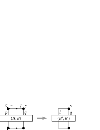
Figure 7: Elementary step for evaluating energies in MPS: Dependence of the energy on one tensor $\gamma$ (see text).

Let us first consider the scenario depicted in Fig. 7: We are given two tensors $G_{pr|pr}$ and $\gamma_{lq|lq}$, where $G_{rr}=0$, i.e. it is in left-canonical form, and $r\triangleright l$ is contracted, and consider a Hamiltonian $(H,E)$ acting on $pq$. Following Eq. (18) for the contraction, using Eq. (20) for the inverse, and rearranging some terms, we find that the contraction yields a CM

$$\Theta=\left(\begin{matrix}G_{pp}&0\\ 0&0\end{matrix}\right)+\left(\begin{matrix}G_{pr}&0\\ 0&\openone\end{matrix}\right)\left(\begin{matrix}\gamma_{ll}&-\gamma_{ql}^{\intercal}\\ \gamma_{ql}&\gamma_{qq}\end{matrix}\right)\left(\begin{matrix}G_{pr}^{\intercal}&0\\ 0&\openone\end{matrix}\right)\>.$$ (48)

We can thus rewrite

$$\mathrm{tr}[H\Theta]$$

$$=\mathrm{tr}\Big{[}H\left(\begin{matrix}G_{pp}&0\\ 0&0\end{matrix}\right)\Big{]}+\mathrm{tr}\Big{[}H\left(\begin{matrix}G_{pr}&0\\ 0&\openone\end{matrix}\right)\gamma\left(\begin{matrix}G_{pr}^{\intercal}&0\\ 0&\openone\end{matrix}\right)\Big{]}$$ (49)

$$=\mathrm{tr}[H_{pp}G_{pp}]+\mathrm{tr}[H^{\prime}\gamma]\ ,$$ (50)

with

$$H^{\prime}=\left(\begin{matrix}G_{pr}^{\intercal}&0\\ 0&\openone\end{matrix}\right)H\left(\begin{matrix}G_{pr}&0\\ 0&\openone\end{matrix}\right)\ ,$$ (51)

where the size of the identities is $|q|\times|q|$, and of course $|r|=|l|$, and therefore $H^{\prime}$ has dimensions $(|l|+|q|)\times(|l|+|q|)$. The effective Hamiltonian acting on the $\gamma$ system – comprised of the modes in $l$ and $q$ – is thus obtained from the old Hamiltonian through

$$(H,E)\mapsto(H^{\prime},E^{\prime}=E+\mathrm{tr}[H_{pp}G_{pp}])$$ (52)

with $H^{\prime}$ from Eq (51).

Note that if the right tensor were canonical and we instead contracted $l\triangleright r$, the signs of the $\openone$’s in Eq. (51) had to be reversed.

IV.2 Energy in GFMPS: Iteration formula

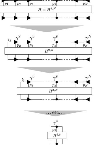
Figure 8: Scheme for the contraction of the Hamiltonian. We proceed stepwise from both ends (here shown from the left end), which gives an effective Hamiltonian for successively smaller patches which also acts on the dangling virtual bonds at the boundary, finally yielding an effective Hamiltonian for $\gamma^{\hat{s}}$.

We are now ready to derive how the energy of a given GFMPS for some Hamiltonian $(H^{1,N},E^{1,N})$, acting on $p_{1},\dots,p_{N}$, depends on the GFMPS tensor at a specific site $\hat{s}$. It is based on iterated application of the elementary step above, and is illustrated in Fig. 8.

Consider an MPS in canonical form around $\hat{s}$, with $H$ acting on all physical sites $p_{1},\dots,p_{N}$. For the description, we assume the generic case $1<\hat{s}<N$, but the procedure is easily applied to any $\hat{s}$. By applying the procedure derived in the last section to $\gamma^{1}$ (corresponding to $G$ above) vs. the remaining tensors (seen as one blocked tensor $\gamma$), we obain an effective Hamiltonian

$$H^{2,N}\stackrel{{\scriptstyle l_{2}\leftarrow r_{1}}}{{=}}(\gamma^{1}_{p_{1}r_{1}}\oplus\openone)^{\intercal}H^{1,N}(\gamma^{1}_{p_{1}r_{1}}\oplus\openone)\ ,$$ (53)

where $H^{2,N}$ is acting on $l_{2},p_{2},\dots,p_{N}$, and we re-label $r_{1}$ to $l_{2}$, as indicated on top of the equality sign. We can repeat this procedure

$$H^{s+1,N}\stackrel{{\scriptstyle l_{s+1}\leftarrow r_{s}}}{{=}}(\gamma^{s}_{l_{s}p_{s}|r_{s}}\oplus\openone)^{\intercal}H^{s,N}(\gamma^{s}_{l_{s}p_{s}|r_{s}}\oplus\openone)\ ,$$ (54)

until we reach site $\hat{s}$.

Similarly, we can contract $H$ from the right, using

$$H^{\hat{s},s-1}\stackrel{{\scriptstyle r_{s-1}\leftarrow l_{s}}}{{=}}(\gamma^{s}_{p_{s}r_{s}|l_{s}}\oplus(-\openone))^{\intercal}H^{\hat{s},s}(\gamma^{s}_{p_{s}r_{s}|l_{s}}\oplus(-\openone))$$ (55)

– note the $-\openone$ due to the opposite contraction order – until we reach $\hat{s}$.

In words, each step removes one site from the MPS and instead updates the way in which the Hamiltonian acts on the dangling virtual leg at the boundary (this update rule thus involves the correlations between this dangling leg and the physical leg in the bulk). This is illustrated for the left boundary in Fig. 8: In order to update $H$, we have to take the Hamiltonian part corresponding to the left+physical leg which are being removed (site $s$), and transform it with $\gamma^{s}_{lp|r}$ which relates those legs to the new dangling leg (and correspondingly from the right).

In order to compute the total energy, we must also keep track of the $E$ contribution. It is updated as

$$E^{s+1,N} =\mathrm{tr}[H^{s,N}_{l_{s}p_{s}|l_{s}p_{s}}\gamma^{s}_{l_{s}p_{s}|l_{s}p_{s}}]+E^{s,N}$$ (56)

$$E^{\hat{s},s-1} =\mathrm{tr}[H^{\hat{s},s}_{p_{s}r_{s}|p_{s}r_{s}}\gamma^{s}_{p_{s}r_{s}|p_{s}r_{s}}]+E^{\hat{s},s}$$

with $E^{2,N}=\mathrm{tr}[H^{1,N}_{p_{1}p_{1}}\gamma^{1}_{p_{1}p_{1}}]=\mathrm{tr}[H_{p_{1}p_{1}}\gamma^{1}_{p_{1}p_{1}}]$, and accordingly $E^{\hat{s},N-1}=\mathrm{tr}[H_{p_{N}p_{N}}\gamma^{N}_{p_{N}p_{N}}]$.

We are thus left with a single-site Hamiltonian $H^{\hat{s},\hat{s}}$ acting on $l_{\hat{s}}p_{\hat{s}}r_{\hat{s}}$, such that the total energy is

$$E_{\mathrm{tot}}(\gamma^{\hat{s}})=\mathrm{tr}[H^{\hat{s},\hat{s}}\gamma^{\hat{s}}]+E^{\hat{s},\hat{s}}\ .$$ (57)

IV.3 Local Hamiltonians

Let us now consider the special case of local Hamiltonians – for simplicity, we consider nearest-neighbor Hamiltonians – and explain how the evaluation of the Hamiltonian in this case can be accomplished in linear time in the system size. Moreover, just as in conventional DMRG, it is possible to store intermediate terms at each cut such that the effort required to update this information when moving by one site is independent of system size.

In the following, it will be convenient to also carry an $l_{1}$ and $r_{N}$ label, with the corresponding spaces being zero-dimensional (in the CM). In any step of the computation, the Hamiltonian will be of the banded form

$$H^{s,N}=\ \blockarray{ccccc}l_{s}&p_{s}p_{s+1}p_{s+2}\dots\\ \block{(c|c|c|c|c)}A^{s}_{\blacktriangleright}B^{s}_{\blacktriangleright}\phantom{\ddots}\\ \BAhline-(B^{s}_{\blacktriangleright})^{\intercal}D^{s}_{\blacktriangleright}+h_{11}h_{12}\phantom{\ddots}\\ \BAhline-h_{12}^{\intercal}h_{22}+k_{11}k_{12}\phantom{\ddots}\\ \BAhline-k_{12}^{\intercal}k_{22}+\dots\ddots\\ \BAhline\ddots\ddots\\ \;\;.$$ (58)

Here, $A^{s}_{\blacktriangleright}$, $B^{s}_{\blacktriangleright}$, and $D^{s}_{\blacktriangleright}$ summarize the information from all sites to the left of $s$, and $h$ ($k$) is the two-site Hamiltonian term acting on sites $p_{s},p_{s+1}$ ($p_{s+1},p_{s+2}$), respectively. One update step Eq. (54) maps this to

$$H^{{s+1},N}=\ \blockarray{cccc}l_{s+1}&p_{s+1}p_{s+2}\dots\\ \block{(c|c|c|c)}A^{s+1}_{\blacktriangleright}B^{s+1}_{\blacktriangleright}\phantom{\ddots}\\ \BAhline-{(B^{s+1}_{\blacktriangleright})}^{\intercal}D^{s+1}_{\blacktriangleright}+k_{11}k_{12}\phantom{\ddots}\\ \BAhline-k_{12}^{\intercal}k_{22}+\dots\ddots\\ \BAhline\ddots\ddots\\ \;\;.$$ (59)

with the update rule

$$A^{s+1}_{\blacktriangleright} =\gamma_{lr}^{\intercal}A^{s}_{\blacktriangleright}\gamma_{lr}+\gamma_{pr}^{\intercal}(D^{s}_{\blacktriangleright}+h_{11})\gamma_{pr}$$ (60)

$$\hskip 40.00006pt+\gamma_{lr}^{\intercal}B^{s}_{\blacktriangleright}\gamma_{pr}-\gamma_{pr}^{\intercal}{(B^{s}_{\blacktriangleright})}^{\intercal}\gamma_{lr}$$

$$B^{s+1}_{\blacktriangleright} =\gamma_{pr}^{\intercal}h_{12}$$

$$D^{s+1}_{\blacktriangleright} =h_{22}$$

where $\gamma\equiv\gamma^{s}$. We thus see that (i) the block-diagonal form of $H^{s,N}$ is preserved, (ii) the initial Hamiltonian is of this form with $A^{1}_{\blacktriangleright}=0$, $B^{1}_{\blacktriangleright}=0$, $D^{1}_{\blacktriangleright}=0$, and (iii) updating the information about the Hamiltonian only requires local updates.

Analogously, we can also keep the integrated Hamiltonian terms for all sites right of $s$ through the update rule

$$A^{s-1}_{\blacktriangleleft} =\gamma_{rl}^{\intercal}A^{s}_{\blacktriangleleft}\gamma_{rl}+\gamma_{pl}^{\intercal}(h_{22}+D^{s}_{\blacktriangleleft})\gamma_{pl}$$ (61)

$$\hskip 40.00006pt+\gamma_{rl}^{\intercal}B^{s}_{\blacktriangleleft}\gamma_{pl}-\gamma_{pl}^{\intercal}{(B^{s}_{\blacktriangleleft})}^{\intercal}\gamma_{rl}$$

$$B^{s-1}_{\blacktriangleleft} =\gamma_{pl}^{\intercal}h_{12}^{\intercal}$$

$$D^{s-1}_{\blacktriangleleft} =h_{11}\ ,$$

where again $\gamma=\gamma^{s}$, and $h$ acts on sites $p_{s-1},p_{s}$ (with $h_{11}$ corresponding to $p_{s-1}$, etc.), starting with $A^{N}_{\blacktriangleleft}=B^{N}_{\blacktriangleleft}=D^{N}_{\blacktriangleleft}=0$.

For a state with working site $\hat{s}$, we find that

$$\hat{H}^{\hat{s},\hat{s}}=\begin{pmatrix}A^{\hat{s}}_{\blacktriangleright}&B^{\hat{s}}_{\blacktriangleright}&0\\ -{(B^{\hat{s}}_{\blacktriangleright})}^{\intercal}&D^{\hat{s}}_{\blacktriangleright}+D^{\hat{s}}_{\blacktriangleleft}&-{(B^{\hat{s}}_{\blacktriangleleft})}^{\intercal}\\ 0&B^{\hat{s}}_{\blacktriangleleft}&A^{\hat{s}}_{\blacktriangleleft}\end{pmatrix}$$ (62)

with mode ordering $lpr$. Similarly, we can compute $E^{\hat{s},\hat{s}}=E^{\hat{s}}_{\blacktriangleright}+E^{\hat{s}}_{\blacktriangleleft}$, where $E^{1}_{\blacktriangleright}=E^{N}_{\blacktriangleleft}=0$, and

$$E^{s+1}_{\blacktriangleright} =E^{s}_{\blacktriangleright}+\mathrm{tr}[H^{s,N}_{l_{s}p_{s}|l_{s}p_{s}}\gamma^{s}_{l_{s}p_{s}|l_{s}p_{s}}]$$ (63)

$$=E^{s}_{\blacktriangleright}+\mathrm{tr}\big{[}\begin{pmatrix}A^{s}_{\blacktriangleright}&B^{s}_{\blacktriangleright}\\ -{(B^{s}_{\blacktriangleright})}^{\intercal}&D_{\blacktriangleright}^{s}+h^{s}_{11}\end{pmatrix}\gamma^{s}_{lp|lp}\big{]}$$

and accordingly

$$E^{s-1}_{\blacktriangleleft}=E^{s}_{\blacktriangleleft}+\mathrm{tr}\big{[}\begin{pmatrix}h^{s-1}_{22}+D_{\blacktriangleleft}^{s}&-{(B^{s}_{\blacktriangleleft})}^{\intercal}\\ B^{s}_{\blacktriangleleft}&A^{s}_{\blacktriangleleft}\end{pmatrix}\gamma^{s}_{pr|pr}\big{]}$$ (64)

where $h^{s}_{11}$ ($h^{s}_{22}$) are the left (right) part of the Hamiltonian term acting between sites $s$ and $s+1$. Overall, the dependence of the energy on $\gamma^{\hat{s}}$ is then given by

$$E_{\mathrm{tot}}(\gamma^{\hat{s}})=\mathrm{tr}[H^{\hat{s},\hat{s}}\gamma^{\hat{s}}]+E^{\hat{s},\hat{s}}\ .$$ (65)

Since all update rules for the $A$, $B$, $D$, and $E$ are local, they can be updated (and thus the energy dependence on $\gamma^{\hat{s}}$ computed) at a cost independent of the system size when moving the working site.

The generalization beyond nearest-neighbor Hamiltonians follows the same pattern illustrated above, but the Hamiltonian of Eq. (58) will have additional off-diagonal terms. In particular, the first row/column, which contains coupling terms between sites $q<s$ and $p\geq s$, will be modified as follows: (i) The terms $A^{s}_{\blacktriangleright}$ and $B^{s}_{\blacktriangleright}$ will contain additional contributions from terms between $q<s$ and $s$, and (ii) there will be additional off-diagonal blocks similar to $B^{s}_{\blacktriangleright}$ for coupling terms between $q<s$ and $p>s$. The update rule (60) is adapted by applying the rule for $B^{s+1}_{\blacktriangleright}$ for all similar off-diagonal terms, and including additional terms in $A^{s+1}_{\blacktriangleright}$. The update for the constant term can be adapted similarly. The total number of blocks that need to be treated in each step depends on the total number of Hamiltonian terms between sites $q<s$ and $p\geq s$.

IV.4 Energy minimization

A core ingredient in DMRG algorithms is the optimization of the energy as a function of a single tensor $\gamma^{\hat{s}}\equiv\gamma$. As we have seen, this energy dependence can be summed up in an effective Hamiltonian $H^{\hat{s},\hat{s}}\equiv H$ and constant offset $E^{\hat{s},\hat{s}}\equiv E$. In order to minimize $E(\gamma)=\mathrm{tr}(H\gamma)+E$, we need to fill all modes with negative energy. This can be done by by going to the eigenbasis of $H$,

$$H\cong\bigoplus_{i}\left(\begin{matrix}0&e_{i}\\ -e_{i}&0\end{matrix}\right)$$ (66)

and choosing

$$\gamma\cong\bigoplus_{i}\left(\begin{matrix}0&1\\ -1&0\end{matrix}\right)\ .$$ (67)

Numerically, this can be done by diagonalizing the antisymmetric matrix $H$ (giving imaginary eigenvalues) and then replacing them by their sign, $\gamma=\mathrm{sign}(H)$, or by following the numerical approaches discussed in Ref. 47.

V GFMPS optimization algorithms

We now describe some commonly used MPS algorithms specifically in the context of GFMPS. Most importantly, we will describe how to carry out the DMRG algorithm in its formulation as a variational method over GFMPS. In addition, we will discuss how to implement the time-dependent variational principle (TDVP), which is suitable for both time evolution and ground state simulations, with GFMPS, as well as a translational invariant version of those methods.

V.1 Gaussian fermionic DMRG

The DMRG algorithm can be naturally described as a variational method over the family of MPS with a given bond dimension. The key idea is to sweep through the system and sequentially optimize a small number (usually one or two) GFMPS tensors in each step. Each such optimization is a quadratic problem and can thus be efficiently solved. In the case where more than one tensor is optimized, the state can be brought back into MPS form using the singular value decomposition. While local convergence does not guarantee global convergence of the energy, this algorithm is empirically found to perform extremely well.

V.1.1 The algorithm

Gaussian fermionic DMRG, i.e. DRMG for a quadratic fermionic Hamiltonian and with GFMPS as a variational family, follows closely the conventional way of doing DMRG with MPS, see e.g. [5; 6]. It consists of an initialization step, followed by a number of sweeps; each sweep in turn consists of a right- and a left-sweep. For concreteness, we will consider the case of a nearest-neighbor Hamiltonian, but the same steps equally apply to more complex Hamiltonians (with suitable modifications regarding the computation of effective Hamiltonians, cf. Sec. IV). The notation follows the one used in the previous sections. In addition, we will denote the complete set of left and right boundary terms that enter the effective Hamiltonian at position $s$ by $\mathcal{B}_{\blacktriangleright}^{s}=\{A^{s}_{\blacktriangleright},B^{s}_{\blacktriangleright},D^{s}_{\blacktriangleright},E^{s}_{\blacktriangleright}\}$ and $\mathcal{B}_{\blacktriangleleft}^{s}=\{A^{s}_{\blacktriangleleft},B^{s}_{\blacktriangleleft},D^{s}_{\blacktriangleleft},E^{s}_{\blacktriangleleft}\}$, respectively. We begin by describing the variant where only one tensor is optimized at a time (”single-site DMRG”).

(i) Initialization.—Fix a bond mode number for each bond $(s,s+1)$, $s=1,\dots,N-1$, and choose a random (pure) initial tensor $\gamma^{s}$ for each site $s$. Let $\mathcal{B}^{N}_{\blacktriangleleft}=\{\varnothing,\varnothing,\varnothing,\varnothing\}$, where by $\varnothing$ we denote a $0\times 0$ matrix.
For $\hat{s}=N,N-1,\dots,2$ do:

1. Bring $\gamma^{\hat{s}}$ into right-canonical form (Sec. III.2).

2. Compute $\mathcal{B}^{\hat{s}-1}_{\blacktriangleleft}$ as given by Eq. (61), and store the result.

After the initialization, we are left with an GFMPS with all tensors in right-canonical form.

(ii) Right-sweep.—Let $\mathcal{B}^{1}_{\blacktriangleright}=\{\varnothing,\varnothing,\varnothing,\varnothing\}$.
For $\hat{s}=1,\dots,N-1$ do:

1. Compute $H^{\hat{s},\hat{s}}$ from $\mathcal{B}^{\hat{s}}_{\blacktriangleright}$ using Eq. (62) (or a suitable modification, based on Sec. IV, for longer ranged Hamiltonians.)

2. Choose $\gamma^{\hat{s}}$ such as to optimize the energy $\mathrm{tr}[H^{\hat{s},\hat{s}}\gamma^{\hat{s}}]$.

3. Bring $\gamma^{\hat{s}}$ into left-canonical form (updating $\gamma^{\hat{s}+1}$ correspondingly).

4. (Re-)compute $\mathcal{B}^{\hat{s}+1}_{\blacktriangleright}$.

(iii) Left-sweep.—The left-sweep works analogous to the right-sweep, just that one iterates over $\hat{s}=N,N-1,\dots,2$, and steps 3 and 4 are replaced by bringing $\gamma^{\hat{s}}$ into right-canonical form and updating $\mathcal{B}^{\hat{s}-1}_{\blacktriangleleft}$, respectively.

To find the ground state, one performs several left- and right-sweeps until convergence is reached. Convergence is typically tested for using the ground state energy (see also our discussion in Sec. VI).

A straightforward generalization of this algorithm is to the ”two-site DMRG” algorithm, which optimizes two adjacent tensors in each step. This coincides with the original DMRG algorithm due to White [3; 4]. Given a GFMPS in canonical form around a center site $\hat{s}$ during a sweep to the right, the tensors on sites $\hat{s},\hat{s}+1$ are optimized by first using the steps laid out in Sec. IV to obtain an effective Hamiltonian $H^{(\hat{s},\hat{s}+1),(\hat{s},\hat{s}+1)}$. One then finds the ground state of this Hamiltonian on the modes $l_{\hat{s}},p_{\hat{s}},p_{\hat{s}+1},r_{\hat{s}+1}$. Using the singular value decomposition of Sec. II.4.1 and absorbing the middle tensor $\Lambda$ into the right tensor, one can put the state back into canonical GFMPS form with a new center site $\hat{s}^{\prime}=\hat{s}+1$; therefore, no extra steps are required to keep the state canonical. When sweeping to the left, the same steps are performed on the sites $\hat{s}-1,\hat{s}$, and in the final SVD $\Lambda$ is absorbed into the left tensor. During the singular value decomposition, the bond dimension can be truncated as appropriate.

In conventional DMRG, the single-site algorithm needs to be augmented with the technique described in Ref. 53. This addresses two issues of the single-site algorithm, namely that the number of states on a bond is difficult to adapt dynamically, and a tendency to become stuck in local minima. While this technique does not have a simple generalization to the GFMPS case, we find in practice that for a fixed bond dimension, the convergence of single- and two-site DMRG on GFMPS is very similar; furthermore, given the much lower cost of the GFMPS-based algorithms, it is often not necessary to dynamically adapt the bond number.

V.1.2 Scaling and efficiency

All steps in the GFDMRG algorithm can be carried out at a cost of $\mathcal{O}\left((\chi+p)^{3}\right)$, where $\chi$ is the number of Majorana modes on each bond and $p$ the number of physical Majorana modes on each site. In practical numerical implementations, the most costly step will usually be the inversion required to contract two tensors, which can be optimized using the block formulas of Eqs. (19,20). The scaling of a single sweep with system size is $\mathcal{O}(N)$. The number of sweeps required to reach convergence heavily depends on the underlying problem and cannot in general be bounded.

Additional cost is incurred if the Hamiltonian is not nearest-neighbor. In particular, the number of additional blocks that need to be included when computing the effective Hamiltonian at site $s$ depends on the number of Hamiltonian terms that couples sites $p<s$ and $q\geq s$. Therefore, the scaling depends crucially on details of the Hamiltonian. In a simple case, such as periodic boundary conditions leading to a single additional term between the left and the right end of the system, the additional cost is constant, while in the most general case of coupling between all sites an additional factor $N^{2}$ could be incurred.

In contrast to conventional DMRG algorithms, the performance can be improved significantly by blocking a group of $n_{b}$ sites together. To understand this, consider a system of $N$ sites with $p$ Majorana modes on each site, and a GFMPS description with Majorana bond number $\chi$. In this case, the matrices of the MPS will be of size $(2\chi+p)\times(2\chi+p)$, and the computational cost of a sweep will scale as $L(2\chi+p)^{3}$. If we group $n_{b}$ sites into one, we instead obtain a scaling of $(L/n_{b})(2\chi+n_{b}p)^{3}$. In general, one has $\chi\gg p$, and optimal performance will be achieved for $n_{b}>1$. For local Hamiltonians, the optimal choice is $n_{b}=\chi/2$. For non-local Hamiltonians, an additional advantage can arise because the Hamiltonian may become less long-ranged if sites are blocked together.

Finally, in the discussion so far we have considered general Gaussian states rather than states with a fixed particle number. In principle, Gaussian states with fixed particle number can be described by matrices that are smaller by a factor of two, thus potentially leading to a speedup of order $2^{3}$.

We will perform a more detailed analysis of the performance for specific models in Sec. VI.2.2.

V.2 TDVP

The time-dependent variational principle (TDVP) can be adapted to use MPS [25] as variational manifold to approximately solve the time-dependent Schrödinger equation both in real and imaginary time. In Ref. 26, it is shown that TDVP can be re-formulated as a modification of the DMRG method, with only a few modifications. In the following, we discuss how to modify the GFDMRG algorithm described above to obtain TDVP for GFMPS following the recipe of Ref. 26.

To perform the evolution for some sufficiently small timestep $t$ (where real time evolution corresponds to real $t$, and imaginary time evolution to $t=i\tau$, $\tau>0$), the steps 2, 3, and 4 in (ii) Right-sweep are replaced by the following sequence: steps :

1. Evolve $\gamma^{\hat{s}}$ under $H^{\hat{s},\hat{s}}$ for time $t$.

2. Perform Step (I) of the elementary move to bring $\gamma^{\hat{s}}$ into left-canonical form, see Sec. III.2 and Fig. 6, i.e. bring $\gamma^{\hat{s}}$ into left-canonical form $\hat{\gamma}^{\hat{s}}$ by splitting off the SVD $\Lambda$, but do not absorb $\Lambda$ in $\gamma^{\hat{s}+1}$ yet.

3. (Re-)compute $\mathcal{B}^{\hat{s}+1}_{\blacktriangleright}$, using the new (left-canonical) $\hat{\gamma}^{\hat{s}}$. (Since $\mathcal{B}^{\hat{s}+1}$ does not depend on $\gamma^{\hat{s}+1}$, this is already the correct $\mathcal{B}^{\hat{s}+1}$.)

4. Compute the effective Hamiltonian $H_{\Lambda}$ for $\Lambda$, which describes the dependence of the energy on $\Lambda$:

   $$H_{\Lambda}=\begin{pmatrix}A^{\hat{s}+1}_{\blacktriangleright}&B^{\hat{s}+1}_{\blacktriangleright}\gamma_{pl}^{\hat{s}+1}\\ {-(B^{\hat{s}+1}_{\blacktriangleright}\gamma_{pl}^{\hat{s}+1})}^{\intercal}&A^{\hat{s}}_{\blacktriangleleft}\end{pmatrix}\ ,$$ (68)

   and evolve $\Lambda$ with $H_{\Lambda}$ for time $-t$.

5. Absorb the evolved $\Lambda$ into $\gamma^{\hat{s}+1}$.

A core ingredient, used in Step 2a and 2b, is to evolve a state $\rho$ with covariance matrix $\Gamma$ with a time-independent Hamiltonian $\mathcal{H}=\mathrm{i}\sum H_{ij}c_{i}c_{j}$ either in real or imaginary time. In the covariance matrix formalism, the Schrödinger equation in real time takes the form

$$\Gamma(0)\mapsto\Gamma(t)=O(t)\Gamma(0)O(t)^{\intercal}\ ,$$ (69)

with $O(t)=\exp(4Ht)$ . For imaginary time, this is replaced by integrating [55]

$$\dot{\Gamma}(t)=-4(H+\Gamma(t)H\,\Gamma(t))\ .$$ (70)

For details on the implementation, such as the optimal choice of time discretization as well as the generalization to a two-site version of the algorithm that allows a dynamical choice of the bond dimension, we refer the reader to Ref. [26]. Note that in the case where $t\to\mathrm{i}\>\infty$, we recover the DMRG algorithm.

V.3 Infinite systems

It was already pointed out in Ref. 3 that DMRG is in principle suitable for infinite systems. While this approach initially enjoyed some success, for a long time DMRG for finite systems was considered more accurate. More recently, however, DMRG for infinite systems has been reinterpreted in the language of matrix product states, which has allowed for accurate and efficient methods for infinite, translationally invariant MPS to be developed [56; 57; 58; 6]. The underlying idea of this reinterpretation is to consider an MPS made up of a unit cell of $K$ sites that repeats indefinitely; in the simplest case, $K=1$, the tensor is the same on each site of the lattice. It turns out that most MPS algorithms can be generalized to such an infinite, translationally invariant ansatz by reformulating them in terms of eigenvectors of transfer operators along the MPS.

While non-interacting systems can be solved directly in the thermodynamic limit by expressing the problem in momentum space, such an approach may scale unfavorably with the number of sites in the unit cell and does not give access to real-space correlation functions without solving for all momenta and transforming back to real space. Therefore, for a large number of sites in the unit cell, a GFMPS approach directly in the thermodynamic limit will be advantageous.

To illustrate how GFMPS can be generalized to the infinite case, we will limit ourselves to the iDMRG algorithm, and restrict the discussion to the aspects which need to adapted in the GFMPS case. However, similar generalizations are also possible for other infinite MPS methods, such as VUMPS [58]. We begin by briefly reviewing the conventional iDMRG algorithm of Ref. 3, where we specialize to the case of a two-site Hamiltonian $H$. Our description follows closely Ref. 6, which we refer to for details. The algorithm proceeds in the following steps:

1. Compute the covariance matrix $\Gamma^{n=1}$ corresponding to the ground state of $H$ on two sites, and perform an SVD such that $\Gamma$ is given as the contraction of three tensors $A^{n}$, $\Lambda^{n}$ and $B^{n}$, where $A^{n}$ and $B^{n}$ are left- and right-canonical MPS tensors, respectively.

2. Extend the lattice by two sites in the middle and consider an MPS where the tensor immediately to the left (right) of the newly inserted sites is given by $A^{n}$ ($B^{n}$). Follow the steps outlined in Sec. IV, especially Eqns. (60)-(62) (adapted for two center sites), to obtain the effective Hamiltonian for the two sites newly added in the center. Use Eqns. (63),(64) to obtain the constant part of the energy.

3. Find the ground state $\Gamma^{n+1}$ of this new effective Hamiltonian and again perform a singular value decomposition to obtain $A^{n+1}$, $\Lambda^{n+1}$ and $B^{n+1}$. Return to step (2).

All of the steps outlined here can be performed using techniques already discussed. Note that this approach effectively simulates a finite system of length $2n$, where $n$ is the number of iterations performed. The energy obtained as the sum of the constant term and the effective Hamiltonian for the center sites is variational for this system of $2n$ sites. One generally finds that for sufficiently large $n$, the tensors converge.

One can now take the tensors obtained in the last step, and use them to form an infinite, translationally invariant MPS [56; 6]. Let $A^{n}$, $\Lambda^{n}$, and $B^{n}$ be the tensors obtained in the last iteration of the infinite DMRG algorithm, and $\Lambda^{n-1}$ the central tensor from the previous iteration. We then define, analogous to Ref. 59,

$$\Gamma^{A} =\left(\Lambda^{n-1}\right)^{-1}\triangleright A^{n} \lambda^{A} =\Lambda^{n}$$ (71)

$$\Gamma^{B} =A^{n}\triangleright\left(\Lambda^{n-1}\right)^{-1} \lambda^{B} =\Lambda^{n-1}.$$ (72)

(In the following, we use the notation $A\triangleright B$ to denote the contraction of tensors; which indices are to be contracted follows from the structure of the tensor network.) Here, $\Lambda^{-1}$ denotes a square rank-2 tensor such that $\Lambda\triangleright\Lambda^{-1}$ yields the maximally entangled state between the two sets of modes. From the SVD, $\Lambda$ is of the form $\Lambda=\bigoplus W(\lambda_{k})$ (see Eq. (30)); for a tensor of this form, the inverse of this sense is given by exchanging the left and right modes (i.e., mapping $\lambda_{k}\to-\lambda_{k}$). This can be verified explicitly using Eqn. (18).

If the state is well-converged and the bond dimension large enough, $\gamma^{L,1}=\lambda^{B}\triangleright\Gamma^{A}\triangleright\lambda^{A}\triangleright\Gamma^{B}$ and $\gamma^{L,2}=\lambda^{A}\triangleright\Gamma^{B}\triangleright\lambda^{B}\triangleright\Gamma^{A}$ will be approximately left-canonical, and $\gamma^{R,1}=\Gamma^{A}\triangleright\lambda^{A}\triangleright\Gamma^{B}\triangleright\lambda^{B}$ and $\gamma^{R,2}=\Gamma^{B}\triangleright\lambda^{B}\triangleright\Gamma^{A}\triangleright\lambda^{A}$ will be approximately right-canonical. Expectation values of local observables, such as the energy on a bond, can be obtained from the observation that the reduced density matrix for the two-site unit cell AB is given by $\left(\lambda^{B}\triangleright\Gamma^{A}\triangleright\lambda^{A}\triangleright\Gamma^{B}\triangleright\lambda^{B}\right)_{p^{A}p^{B}|p^{A}p^{B}}$, where the physical indices in the subscript refer to the physical indices of $\Gamma^{A}$ and $\Gamma^{B}$. Note that for the average energy, one must compute the energy for the AB and BA unit cells separately and average.

VI Numerical results

Below we test our numerical implementation of the algorithms presented in the previous sections for three relevant cases: We first study a one-dimensional system that exhibits non-trivial spatial correlation functions, but can be exactly solved, thus providing a simple comparison. Then we turn to a two-dimensional system, which we solve on quasi-two-dimensional cylinder geometries, to assess how accurately our approach works beyond a strictly one-dimensional system and when it performs better than exact approaches. Finally, we study charge transport through a quantum point contact in a simple geometry at finite bias voltage to demonstrate the capability of TDVP to compute dynamical properties of nanostructures.

While the models discussed in this section preserve particle number, we use the Majorana formalism described throughout this manuscript without exploiting particle number conservation.

VI.1 The resonant level model

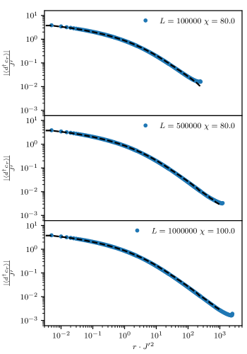
Figure 9: Rescaled real-space correlation function $\langle d^{\dagger}c_{r}\rangle$ of the ground state of Eqn. (73) as a function of (rescaled) distance $r\cdot J^{\prime 2}$. Other parameters are $J^{\prime}=0.05J$ and the number of sites per block $n_{b}=\chi/2$ (see Sec. V.1.2). $\chi$ denotes the maximum Majorana bond number, and $L$ is the size of the system including the impurity. Dashed lines indicate a fit to the exact solution (75).

First, we consider a one-dimensional system which still exhibits non-trivial real-space correlation functions: the resonant-level model, which appears as the non-interacting limit of a number of impurity models (see, e.g., Refs. 60; 61; 62; 63). Here, we follow the discussion of Ref. 64. We consider a fermionic impurity with a corresponding creation operator $d^{\dagger}$ coupled to a bath of fermions, which here is represented by a periodic chain of $L$ fermions with associated creation operators $c_{i}^{\dagger}$. The Hamiltonian is given by

$$H = J^{\prime}\left(d^{\dagger}c_{1}+c_{1}^{\dagger}d\right)+JT_{\rm chain}$$ (73)

$$T_{\rm chain} = \sum_{i}^{L-1}\left(c_{i}^{\dagger}c_{i+1}+c_{i+1}^{\dagger}c_{i}\right)+\left(c_{L}^{\dagger}c_{1}+c_{1}^{\dagger}c_{L}\right)$$ (74)

Here, $T$ is the kinetic energy operator on the chain and $J$ sets the bandwidth; we set the unit of energy to $J=1$ and fix the system to half filling, leaving $J^{\prime}$ as the only free parameter aside from system size.

The quantity of interest is the correlation between the impurity site and the sites in the bath, $C(r)=\langle d^{\dagger}c_{r}\rangle/J^{\prime}$. Owing to the non-interacting nature of the problem, this correlation function can be computed exactly in the thermodynamic limit (assuming a constant density of states around the Fermi energy) and at zero temperature is found to be given by

$$C(r) = Af(BJ^{\prime 2}r)$$ (75)

$$f(\kappa) = -\pi\int_{-\infty}^{\infty}dx\frac{x\cos(\kappa x)+\sin(\kappa x)}{(x^{2}+1)(1+\delta(x))}.$$ (76)

The constants $A$ and $B$ are independent of $L$ and $J^{\prime}$, but depend on the microscopic choice for the bath such as the Fermi velocity and density of states at the Fermi energy, and are taken as fit parameters here; however, they can be computed exactly for certain choices of the bath [64]. The relevant universal behavior is that $C(r)$ shows a characteristic crossover from short-distance to long-distance behavior around $\kappa=BJ^{\prime 2}r\approx 1$; for $\kappa\ll 1$, $f(\kappa)\sim\ln(\kappa)+\gamma$, while for $\kappa\gg 1$, $f(\kappa)\sim 1/\kappa$.

In the previous literature, this crossover was illustrated by collapsing many datasets for different values of $J^{\prime}$, each covering a different range of $\kappa$. Since we are able to study systems almost three orders of magnitude larger than previously possible, we can exhibit the full scaling form in a single dataset. This is shown in Fig. 9. Here, $\chi$ denotes the maximum number of Majorana modes on the bonds of the MPS. This corresponds to a conventional bond dimension of $D(\chi)=\sqrt{2}^{\chi}$; for $\chi=80$, this works out to $D\approx 10^{12}$, and for $\chi=100$ to $D\approx 10^{15}$. The dashed line indicates the exact solution of Eqn. (75) with $A$, $B$ chosen as best fit to the MPS data. We see that agreement is essentially exact up to the largest distances, which are weakly affected by finite-size effects.

VI.2 Quasi-two-dimensional systems

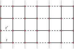
Figure 10: Lattice used to define the 2d Hamiltonian Eqn. (77). Solid lines indicate bonds with strength $t$, and dashed lines indicate bonds with strength $t^{\prime}$. For $t^{\prime}=t$, the square lattice is recovered, while for $t^{\prime}=0$ the brickwall representation of the honeycomb lattice is obtained. The dotted lines indicate periodic boundary conditions in one direction, effectively wrapping the system onto a cylinder.

For a more challenging test, we turn to a model of spinless fermions hopping on a two-dimensional lattice,

$$H_{\rm hop}=-\sum t_{xy}^{x^{\prime}y^{\prime}}\left(c_{xy}^{\dagger}c_{x^{\prime}y^{\prime}}+c_{x^{\prime}y^{\prime}}^{\dagger}c_{xy}\right)$$ (77)

where $c_{xy}^{\dagger}$ creates a fermion on the $x$’th ($y$’th) site in the horizontal (vertical) direction, and the hopping elements $t_{xy}^{x^{\prime}y^{\prime}}$ are chosen to give rise to the brickwall lattice as sketched in Fig. 10. There are three particular limits of this model that we are interested in: (1) The limit where $t^{\prime}=t$, where the system simply becomes the square lattice; (2) the limit of $t^{\prime}=0$, where it becomes the brickwall lattice, whose connectivity equals that of the honeycomb lattice; and (3) the limit of $t=0$, where it becomes a lattice of isolated dimers.

From the point of view of a matrix-product state description, the most relevant property of the system is its entanglement structure, which differs significantly between these three limits. Most easily understood is the case of isolated dimers: in this case, the spectrum is fully gapped with a gap of $2t$, and there is only entanglement between the sites that together form a dimer, and no entanglement (or correlations) otherwise. The state thus has a very simple MPS description. Upon adding the $t$ term and interpolating to the square lattice limit $t=t^{\prime}$, the gap decreases and finally the system becomes gapless at $t=t^{\prime}$. Correspondingly, the entanglement increases. The square lattice hosts a gapless state with one-dimensional Fermi surface. This leads to a logarithmic violation of the area law [65; 66; 67; 68] and thus represents the most difficult case for a tensor network state approach. Finally, in the case of the brickwall/honeycomb lattice, the system is gapless, but with Dirac points instead of Fermi surfaces. In this limit, the entanglement follows an area law despite the gapless nature of the system.

In the following, we will focus on the case of the honeycomb/brickwall lattice, and defer a discussion of the other cases to Appendix A. Due to the area law in the honeycomb/brickwall case, the maximum entropy that must be captured in the MPS scales linearly in its width $W$. We therefore choose $\chi$ proportional to the width of the system $W$.

For the numerical simulations using DMRG methods, we study this lattice on cylinders of circumference $W$ and length $L$, i.e. with a total of $W\cdot L$ sites. We map the sites to a chain following each rung (of length $W$) from bottom to top. We have found that the single-site and two-site optimization algorithm generally lead to comparable results, and thus use the single-site algorithm throughout. We perform at least 5 sweeps and terminate when the absolute change in energy between sweeps drops below $10^{-3}$.

VI.2.1 Convergence of real-space correlation functions

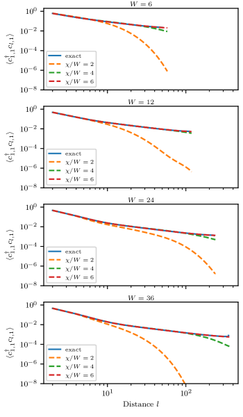
Figure 11: Real-space correlation functions for the ground state of Eqn. (77) with $t=1$, $t^{\prime}=0$. Correlations are shown between two sites of the same (odd) vertical position and different horizontal positions, i.e. probing the decay of correlations along the cylinder. These results are obtained using the single-site optimization algorithm with $W$ sites blocked into one for systems of aspect ratio 10, i.e. $L=10W$. Exact results are obtained from a full diagonalization of the same system.

To characterize how well the MPS ground state approximates the exact one, we study the real-space correlations. Fig. 11 shows the decay of the equal-time Green’s function along the long direction of the cylinder in the limit of a brickwall/honeycomb lattice, $t^{\prime}=0$. Here, we scale the Majorana bond number with the width of the cylinder, showing $\chi=2W,4W,6W$. This choice is motivated by the area law.

It is well-known that for finite bond dimension, correlations in an MPS decay exponentially at sufficiently long distances [1]. At shorter distances, the correlations can approximate a polynomial decay. This is clearly borne out in the data of Fig. 11: for small Majorana bond number $\chi$, the correlations exhibit an artificial and unphysical exponential decay, while for sufficiently large $\chi$ the exact polynomial decay $\mathcal{O}(1/l)$ is recovered to high accuracy.

VI.2.2 Performance comparison against exact methods

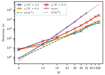
Figure 12: Run time to a converged solution for the ground state of Eqn. (77) with $t=1$, $t^{\prime}=0$ for aspect ratio $L=20W$, i.e. the largest system has $60^{2}\cdot 20=72{,}000$ sites. The dashed line indicates a best fit of the GFMPS data for $\chi/W=6$ to $aW^{4}$, with $a$ a fit parameter, and the dotted line is a best fit of the exact method to $aW^{6}$. These simulations are performed on 4 cores of an Intel(R) Xeon(R) E5-2690 v3 @ 2.60GHz.

We now examine the runtime of the MPS algorithm for quasi-one-dimensional systems compared to exact, full diagonalization methods. Of course absolute run-times are implementation-specific and, in particular in the case of MPS methods, may depend sensitively on details such as the choice of initial states, convergence criterion and many others. More pertinent is therefore an analysis of the scaling of the method.

Exact methods based on fully diagonalizing the hopping matrix of the underlying problem will scale as the cube of the matrix size, i.e. in the case at hand as $\mathcal{O}(W^{3}L^{3})$. Estimating the cost of the MPS method is more challenging since in general, we cannot make any strong assertions on the convergence with the number of sweeps  or the bond dimension. However, we can quantify the cost of a single sweep for fixed bond dimension. As stated in Sec. V.1.2, the cost is $(N/n_{b})(2\chi+n_{b}p)^{3}D$, where $N$ is the number of sites, $p$ the number of Majorana modes per site, $n_{b}$ the number of physical sites that are grouped into one site of the MPS, $\chi$ the Majorana bond number, and $D$ the number of operators that must be tracked to accomodate long-range hopping terms, which depends on the details of the Hamiltonian and $n_{b}$. For the case of a quasi-1d system at hand, as we have seen above, to achieve fixed accuracy we scale $\chi\sim W$, and block a number of sites $n_{b}=\chi/2$ for optimal performance; therefore, $n_{b}\sim W$. For this case, it turns out that $D$ is a constant independent of $W$. Therefore, the overall scaling becomes $LW^{3}$. For the case where we fix the aspect ratio, $L\sim W$, we thus obtain a scaling of $\mathcal{O}(W^{6})$ for the exact methods and $\mathcal{O}(W^{4})$ for the MPS method.

The memory usage of the exact method scales as $(WL)^{2}$, while the GFMPS approach scales as $(WL/n_{b})(2\chi+n_{b}p)^{2}$. For the choices made above ($W\sim L,\chi,n_{b}$), this leads to the exact method scaling as $W^{4}$ and the GFMPS approach scaling as $W^{3}$. In practice, given our choice of aspect ratio, the memory requirements of the exact approach are much greater than the GFMPS approach, and turn out to be the limiting factor.

We numerically confirm the scaling of the runtime in Fig. 12, where we show the time to achieve a converged solution instead of the time to perform a single sweep. The GFMPS approach shows polynomial scaling consistent with $W^{4}$ across a range of bond dimensions. This is consistent with the empirical expectation that the number of sweeps scales at most very weakly with the size of the system.

For the parameters chosen here and our implementation, the crossover where the GFMPS method becomes faster than exact approaches is around $W=14$. This is most strongly influenced by the aspect ratio: upon approaching the one-dimensional limit, the GFMPS approach will become more and more favorable.

VI.3 Transport through a quantum point contact

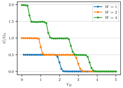
Figure 13: GFMPS simulation of the quantized conductance across a Gaussian potential barrier of height $V_{B}$ in a $W\times 500$ system. For details, see main text.

To illustrate the power of the time-dependent variational principle applied to GFMPS, we study a simple transport problem, namely the quantization of conductance through a quantum point contact in a multi-channel wire [70]. We model the system as a square lattice of spinless fermions of size $W\times L$, i.e. as shown in Fig. 10 with hopping Hamiltonian (77) for $t^{\prime}=t=1$ . We add an on-site potential

$$H_{\rm pot}=\sum\left[-\mu_{0}+V_{B}\exp\left(-\frac{(x-L/2)^{2}}{d^{2}}\right)\right]n_{xy}$$ (78)

where $n_{xy}=c_{xy}^{\dagger}c_{xy}$. This corresponds to a Gaussian potential barrier of height $V_{B}$ and width $d$ at the center of the system in $x$ direction, and independent of $y$.

We initialize the system in the ground state of $H_{\rm hop}+H_{\rm pot}$ using the single-site DMRG algorithm and then apply a voltage $V$ by evolving under the Hamiltonian $H_{\rm hop}+H_{\rm pot}+H_{\rm bias}$ with

$$H_{\rm bias}=\frac{V}{2}\sum_{y}\left(\sum_{x=1}^{L/2-4d}n_{xy}-\sum_{x=L/2+4d}^{L}n_{xy}\right).$$ (79)

Here, we use the sites that are more than $4d$ away from the center of the barrier as leads and apply a symmetric bias voltage, and consider the region between the leads as the quantum point contact. We then meausure the charge in the left half of the system, $N_{\rm left}=\sum_{y}\sum_{x=1}^{L/2}c_{xy}^{\dagger}c_{xy}$, as a function of time. Due to conservation of charge, we can compute the current flowing across the junction as $J(t)=dN_{\rm left}/dt$. Alternatively, we could evaluate the charge operator across the junction.

After a transient time of order $d$, the current settles to a plateau value that will last until the charge transport reaches the end of the leads after a time of order $L$. We compute the average current $\bar{J}$ over this plateau, and define the conductance as $G=\bar{J}/V$. According to well-known theoretical calculations, in the limit of a smooth barrier the conductance should be quantized as $G=NG_{0}/2$, where $N$ is the number of conducting spin channels (i.e., for a usual spin-degenerate system, $N=2K$ with $K$ the number of spinful channels, but here we consider a spinless system) and $G_{0}=2e^{2}/h$. We use units where $e=\hbar=1$, and thus $G_{0}=1/\pi$.

For $V_{B}=0$, we expect the system to have $W$ conducting channels and thus $G=WG_{0}/2$; as we increase the barrier height, the number of channels is reduced one by one as the lowest-momentum channels are cut off first. We confirm this behavior in Fig. 13 for a system with $W=4$, $L=500$, $d=10$, and applied bias voltage $V=0.1$. Our simulations are performed with a GFMPS of Majorana bond number $\chi=50$ and with $n_{b}=W$, and TDVP is run with a timestep of $dt=0.05$. We also note that since the Hamiltonian is time-independent after the quench, a time $t$ can be reached in one step for exact simulations while requiring $t/dt$ steps in TDVP; however, one can easily generalize the TDVP simulation to a time-dependent Hamiltonian, as would arise for example when computing the ac conductance, without incurring additional computational cost.

VII Conclusions

In this paper, we have studied how to apply the DMRG algorithm and other MPS-based algorithms to the simulation of systems of non-interacting fermions. By combining the advantages of the exponentially compressed description of non-interacting fermionic states in terms of second moments and the efficient description of states with bounded (area-law) entanglement through Matrix Product States, we were able to simulate systems far beyond what is possible with either method alone. The central insight of our GFDMRG algorithm is the use of a suitable canonical form, which allows to express the minimization of the energy as a function of a given tensor as an eigenvalue problem, much like in conventional DMRG. This enabled us to realize the variational algorithm for non-interacting fermions in close analogy to the conventional MPS-based formulation of DMRG, as well as to generalize the method to other MPS-based algorithms such as TDVP for time evolution or iDMRG for infinite systems.

The computational cost of the GFDMRG method scales as $L\chi^{3}$ per sweep, with $L$ the length of the chain and $\chi$ the number of modes per bond. Due to the exponential compression of the representation in terms of second moments, the effective bond dimension is $D=2^{\chi/2}$. This allows us to simulate even systems with an amount of entanglement that grows faster than an area law, such as a Fermi surface or states after a quantum quench, efficiently and to high accuracy for very large system sizes. We have demonstrated the power of our method for both one-dimensional and quasi-2D systems, and obtained results for up to one million lattice sites and effective bond dimensions of $10^{15}$.

An interesting follow-up question is how to generalize the method to two-dimensional systems using Projected Entangled Pair States (PEPS). A key point to be addressed is that in our 1D algorithm, the canonical form serves a more central role than in conventional MPS simulations: While in the latter case, the canonical form is primarily used to stabilize the method, in our case it is the key ingredient which allows us to express the dependence of the energy on a tensor as an eigenvalue problem in the first place. Therefore, generalizing the method to 2D requires either to understand how to solve the energy optimization problem without using a canonical form, or consider more specialized two-dimensional tensor networks that have a canonical form.

Appendix A Real-space correlations in the presence of a Fermi surface

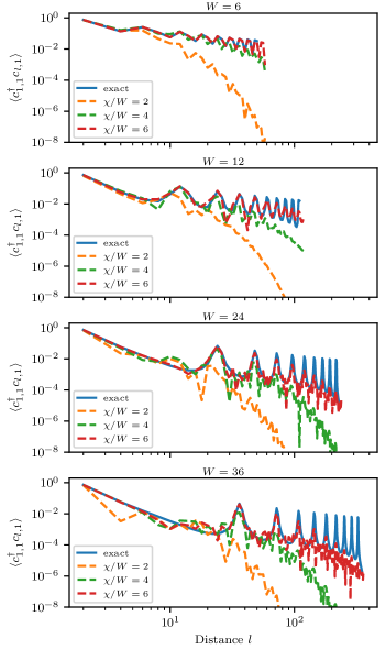
Figure 14: Convergence of real-space correlations functions for the ground state of Eq. 77 in the limit of a square lattice, $t=t^{\prime}$.

In Fig. 14, we show the real-space correlation functions, analogous to Fig. 11, for the case of fermions hopping on the square lattice, i.e. $t=t^{\prime}$. While these exhibit much more structure than the correlations in the honeycomb case, which is due to the interplay of finite Fermi momentum $k_{F}$ and the quantization of momentum around the periodic direction of the cylinder, they still have an envelope that decays as a power-law. Importantly, in contrast to the honeycomb case of Fig. 11, the system violates the area law and thus an accurate description requires a $\chi$ that grows faster than $W$. This can be seen in the data: while for $W=6$, $\chi/W=6$ is sufficient to accurately describe the correlations, for $W=36$ the same $\chi/W$ can not capture the correlations accurately beyond a distance of roughly $10^{2}$.

Appendix B Computation of overlaps of GFMPS

Figure 15: Overlap of GFMPS. The overlap is obtained by contracting the GFMPS with tensors $\gamma^{s}$ and the particle-hole transformed GFMPS with tensors $-\Gamma^{s}$. The contraction can be carried out efficiently by contracting, say, from left to right, in each step contracting first the upper and then the lower MPS tensor to a left boundary tensor. In each step, the opposite contraction order in the lower part must be observed.

In this appendix, we describe how to efficiently evaluate the absolute value squared of the overlap of two GFMPS. We focus on this instead of the overlap itself since the phase of the overlap is not fully determined by a Gaussian covariance matrix; to see this, note that the covariance matrix of two Gaussian states $|\phi\rangle$ and $e^{i\theta}|\phi\rangle$ is the same. For a more detailed discussion of this issue and possible solutions, see Ref. 45.

We begin by slightly generalizing the contraction formalism introduced in Sec. II.2. In particular, Eq. (18) can be generalized to the contraction of two indices $b$, $c$ on a given covariance matrix $\gamma$ even when there is correlation between the two, i.e. $\gamma_{bc|bc}\neq 0$. This should be contrasted with the case of Eq. (18), where the input covariance matrix is the direct sum of two parts and the indices being contracted have no correlations. Starting from the covariance matrix $\gamma_{abc|abc}$, the CM after contracting $b\triangleright c$ is given by

$$K=\gamma_{aa}+\gamma_{a|bc}\left(\gamma_{bc|bc}+\begin{pmatrix}0&\openone\\ -\openone&0\end{pmatrix}\right)^{-1}\gamma_{a|bc}^{\intercal}\ .$$ (80)

Given two states $\rho$ and $\sigma$ with CMs $\gamma_{\rho}$ and $\gamma_{\sigma}$, their overlap is $\mathrm{tr}(\rho\sigma)=2^{-\chi/2}\sqrt{\det(\openone-\gamma_{\rho}\gamma_{\sigma})}$, where $\chi$ is the number of Majorana modes [46], cf. also Eq. (10). From this we can immediately infer that the change in normalization induced by contracting two indices $b\triangleright c$ of a state with CM $\gamma_{abc|abc}$ – which is equivalent to projecting $bc$ on a maximally entangled state – is given by

$$\mathcal{N}=2^{-\chi/2}\sqrt{\left|\det\left[\gamma_{bc|bc}+\left(\begin{smallmatrix}&\openone\\ -\openone\end{smallmatrix}\right)\right]\right|}\ ,$$ (81)

with $\chi=|b|=|c|$ (this can be seen by multiplying with $\Big{(}\begin{smallmatrix}&\openone\\ -\openone\end{smallmatrix}\Big{)}$ in the determinant); note that this exactly corresponds to the determinant of the inverse in the Schur complement in the contraction Eq. (80). This normalization also holds for the case $|a|=0$, i.e. when all indices are contracted.

In order to compute the overlap of two Gaussian states with covariance matrices $\gamma$ and $\Gamma$, we can form the joint covariance matrix $\left(\begin{smallmatrix}\gamma\\ &-\Gamma\end{smallmatrix}\right)$ and contract all indices using Eq. (81); note that in that case $\mathcal{N}$ is independent of the direction of the contraction (i.e., replacing $\openone\leftrightarrow-\openone$). The minus sign reflects the fact that contracting as defined here involves a particle-hole transformation on $\Gamma$ (corresponding to particle number conservation of the maximally entangled state $\omega$ onto which the bond is projected). To compute the overlap of two GFMPS – cf. Fig. 15 – we can perform the same procedure iteratively by contracting the two GFMPS together from left to right. In each step, the change in normalization must be tracked according to Eq. (81). Furthermore, the particle-hole transformation on the second MPS requires to reverse the direction of the contraction of its virtual indices. A convenient way to carry out the procedure is to perform the following contractions:

1. $L^{(1)}=(-\Gamma^{1})\triangleright\gamma^{1}$

2. $L^{\prime}=L^{(n)}\triangleright\gamma^{(n+1)}$

3. $L^{(n+1)}=(-\Gamma^{(n+1)})\triangleright L^{\prime}$ and return to step 2.

Here, in slight abuse of previous notation, we use the symbol $\triangleright$ to denote the (directional) contraction of two tensors (rather than indices), where the correct indices to contract are specified in Fig. 15. In each contraction, including the very last one, the normalization factor $\mathcal{N}$ is tracked; the overall normalization of the overlap is then given by the product of all normalizations. We denote this overlap as $\mathcal{N}(\gamma^{s},\Gamma^{s})$.

One can then obtain the normalized overlap of the two states as

$$|\langle\gamma|\Gamma\rangle|^{2}=\frac{\mathcal{N}(\gamma^{s},\Gamma^{s})}{\sqrt{\mathcal{N}(\gamma^{s},\gamma^{s})\mathcal{N}(\Gamma^{s},\Gamma^{s})}}\ .$$ (82)

The computation of the denominator is greatly simplified by transforming each GFMPS into the left- or right-canonical form. If the left-canonical gauge is chosen for all tensors, then $\gamma^{s}_{rr}=0$, yielding a normalization $2^{-\chi/2}$ for the contraction of a bond with $\chi$ Majorana modes, and thus

$$\mathcal{N}(\gamma^{s},\gamma^{s})=\prod_{i}2^{-\chi^{\gamma}_{i,i+1}/2}$$ (83)

with $\chi^{\gamma}_{i,i+1}$ the bond number at link $(i,i+1)$.

References

- Fannes et al. [1992] M. Fannes, B. Nachtergaele, and R. F. Werner, Communications in Mathematical Physics 144, 443 (1992).
- Östlund and Rommer [1995] S. Östlund and S. Rommer, Phys. Rev. Lett. 75, 3537 (1995).
- White [1992] S. R. White, Phys. Rev. Lett. 69, 2863 (1992).
- White and Noack [1992] S. R. White and R. M. Noack, Phys. Rev. Lett. 68, 3487 (1992).
- Schollwöck [2005] U. Schollwöck, Rev. Mod. Phys. 77, 259 (2005).
- Schollwöck [2011] U. Schollwöck, Annals of Physics 326, 96 (2011).
- Sierra and Martin-Delgado [1998] G. Sierra and M. A. Martin-Delgado, Preprint (1998), arXiv:cond-mat/9811170 .
- Nishino and Okunishi [1998] T. Nishino and K. Okunishi, Journal of the Physical Society of Japan 67, 3066 (1998).
- Nishino et al. [2000] T. Nishino, K. Okunushi, Y. Hieida, N. Maeshima, and Y. Akutsu, Nucl. Phys. B 575, 504 (2000).
- Nishio et al. [2004] Y. Nishio, N. Maeshima, A. Gendiar, and T. Nishino, Preprint (2004), arXiv:cond-mat/0401115 .
- Verstraete and Cirac [2004] F. Verstraete and J. I. Cirac, Preprint (2004), arXiv:cond-mat/0407066 .
- Jordan et al. [2008] J. Jordan, R. Orús, G. Vidal, F. Verstraete, and J. I. Cirac, Phys. Rev. Lett. 101, 250602 (2008).
- Vidal [2007a] G. Vidal, Phys. Rev. Lett. 99, 220405 (2007a).
- Vidal [2008] G. Vidal, Phys. Rev. Lett. 101, 110501 (2008).
- Orús [2014a] R. Orús, Annals of Physics 349, 117 (2014a).
- Orús [2014b] R. Orús, The European Physical Journal B 87, 280 (2014b).
- Bridgeman and Chubb [2017] J. C. Bridgeman and C. T. Chubb, J. Phys. A: Math. Theor. 50, 223001 (2017), arXiv:1603.03039 .
- Kraus et al. [2010] C. V. Kraus, N. Schuch, F. Verstraete, and J. I. Cirac, Phys. Rev. A 81, 052338 (2010).
- Schuch et al. [2012] N. Schuch, M. M. Wolf, and J. I. Cirac, Preprint (2012), arXiv:1201.3945 .
- Dubail and Read [2015] J. Dubail and N. Read, Phys. Rev. B 92, 205307 (2015).
- Haegeman et al. [2013] J. Haegeman, T. J. Osborne, H. Verschelde, and F. Verstraete, Phys. Rev. Lett. 110, 100402 (2013).
- Fishman and White [2015] M. T. Fishman and S. R. White, Phys. Rev. B 92, 075132 (2015).
- Evenbly and White [2016] G. Evenbly and S. R. White, Phys. Rev. Lett. 116, 140403 (2016).
- Haegeman et al. [2018] J. Haegeman, B. Swingle, M. Walter, J. Cotler, G. Evenbly, and V. B. Scholz, Phys. Rev. X 8, 011003 (2018).
- Haegeman et al. [2011] J. Haegeman, J. I. Cirac, T. J. Osborne, I. Pižorn, H. Verschelde, and F. Verstraete, Phys. Rev. Lett. 107, 070601 (2011).
- Haegeman et al. [2016] J. Haegeman, C. Lubich, I. Oseledets, B. Vandereycken, and F. Verstraete, Phys. Rev. B 94, 165116 (2016).
- Weiße et al. [2006] A. Weiße, G. Wellein, A. Alvermann, and H. Fehske, Rev. Mod. Phys. 78, 275 (2006).
- Thouless and Kirkpatrick [1981] D. J. Thouless and S. Kirkpatrick, Journal of Physics C: Solid State Physics 14, 235 (1981).
- Lewenkopf and Mucciolo [2013] C. H. Lewenkopf and E. R. Mucciolo, Journal of Computational Electronics 12, 203 (2013).
- Datta [2000] S. Datta, Superlattices and microstructures 28, 253 (2000).
- Gaury et al. [2014] B. Gaury, J. Weston, M. Santin, M. Houzet, C. Groth, and X. Waintal, Physics Reports 534, 1 (2014), numerical simulations of time-resolved quantum electronics.
- Goedecker [1999] S. Goedecker, Rev. Mod. Phys. 71, 1085 (1999).
- Eisert et al. [2010] J. Eisert, M. Cramer, and M. B. Plenio, Rev. Mod. Phys. 82, 277 (2010).
- Hastings [2007a] M. Hastings, J. Stat. Mech. , P08024 (2007a), arXiv:0705.2024 .
- Arad et al. [2017] I. Arad, Z. Landau, U. Vazirani, and T. Vidick, Commun. Math. Phys. 356, 65 (2017), arXiv:1602.08828 .
- Huang [2014] Y. Huang, (2014), arXiv:1403.0327 .
- White [1998] S. R. White, Physics Reports 301, 187 (1998).
- Verstraete and Cirac [2006] F. Verstraete and J. I. Cirac, Phys. Rev. B 73, 094423 (2006).
- Hastings [2007b] M. B. Hastings, Phys. Rev. B 76, 035114 (2007b).
- Schuch et al. [2008] N. Schuch, M. M. Wolf, F. Verstraete, and J. I. Cirac, Phys. Rev. Lett. 100, 030504 (2008).
- Botero and Reznik [2003] A. Botero and B. Reznik, Phys. Rev. A 67, 052311 (2003).
- Vidal et al. [2003] G. Vidal, J. I. Latorre, E. Rico, and A. Kitaev, Phys. Rev. Lett. 90, 227902 (2003).
- Peschel [2003] I. Peschel, Journal of Physics A: Mathematical and General 36, L205 (2003).
- Botero and Reznik [2004] A. Botero and B. Reznik, Physics Letters A 331, 39 (2004).
- Bravyi and Gosset [2017] S. Bravyi and D. Gosset, Communications in Mathematical Physics 356, 451 (2017).
- Bravyi [2004] S. Bravyi, Preprint (2004), arXiv:quant-ph/0404180 .
- Wimmer [2012] M. Wimmer, ACM Transactions on Mathematical Software (TOMS) 38, 30 (2012).
- Löwdin [1955] P.-O. Löwdin, Phys. Rev. 97, 1474 (1955).
- Giedke and Cirac [2002] G. Giedke and J. I. Cirac, Phys. Rev. A 66, 032316 (2002), quant-ph/0204085 .
- Eisert et al. [2002] J. Eisert, S. Scheel, and M. B. Plenio, Phys. Rev. Lett. 89, 137903 (2002), quant-ph/0204052 .
- Fiurášek [2002] J. Fiurášek, Phys. Rev. Lett. 89, 137904 (2002), quant-ph/0204069 .
- Note [1] This can also be seen without calculation by noting that this amounts to a postselected teleportation protocol (i.e. attaching a maximally entangled state and projecting onto the maximally entangled state).
- White [2005] S. R. White, Phys. Rev. B 72, 180403 (2005).
- Note [2] This can be shown by observing that Eq. (69\@@italiccorr) is equivalent to and thus , and on the other hand comparing it with the evolution of in the Heisenberg picture.
- Kraus and Cirac [2010] C. V. Kraus and J. I. Cirac, New Journal of Physics 12, 113004 (2010).
- McCulloch [2008] I. P. McCulloch, Preprint (2008), arXiv:0804.2509 .
- Crosswhite et al. [2008] G. M. Crosswhite, A. C. Doherty, and G. Vidal, Phys. Rev. B 78, 035116 (2008).
- Vanderstraeten et al. [2019] L. Vanderstraeten, J. Haegeman, and F. Verstraete, SciPost Phys. Lect. Notes , 7 (2019).
- Vidal [2007b] G. Vidal, Phys. Rev. Lett. 98, 070201 (2007b).
- Anderson [1961] P. W. Anderson, Phys. Rev. 124, 41 (1961).
- Toulouse [1970] G. Toulouse, Phys. Rev. B 2, 270 (1970).
- Schlottmann [1980] P. Schlottmann, Phys. Rev. B 22, 613 (1980).
- Filyov et al. [1981] V. Filyov, A. Tzvelik, and P. Wiegmann, Physics Letters A 81, 175 (1981).
- Ghosh et al. [2014] S. Ghosh, P. Ribeiro, and M. Haque, Journal of Statistical Mechanics: Theory and Experiment 2014, P04011 (2014).
- Wolf [2006] M. M. Wolf, Phys. Rev. Lett. 96, 010404 (2006).
- Gioev and Klich [2006] D. Gioev and I. Klich, Phys. Rev. Lett. 96, 100503 (2006).
- Barthel et al. [2006] T. Barthel, M.-C. Chung, and U. Schollwöck, Phys. Rev. A 74, 022329 (2006).
- Li et al. [2006] W. Li, L. Ding, R. Yu, T. Roscilde, and S. Haas, Phys. Rev. B 74, 073103 (2006).
- Note [3] See Ref. \rev@citealpnumlandau2015polynomial for an MPS-based variational method where convergence can be guaranteed in certain cases.
- Nazarov et al. [2009] Y. V. Nazarov, Y. Nazarov, and Y. M. Blanter, Quantum transport: introduction to nanoscience (Cambridge university press, 2009).
- Landau et al. [2015] Z. Landau, U. Vazirani, and T. Vidick, Nature Physics 11, 566 (2015).