Dynamics of phases and chaos in models of locally coupled conservative or dissipative oscillators

Abstract

We discuss Hamiltonian model of oscillator lattice with local coupling. Model describes spatial modes of nonlinear Schrödinger equation with periodic tilted potential. The Hamiltonian system manifests reversibility of Topaj – Pikovsky phase oscillator lattice. Furthermore, the Hamiltonian system has invariant manifolds with dynamics exactly equivalent to the Topaj – Pikovsky model. We demonstrate the complexity of dynamics with results of numerical simulations. We also propose two dissipative models close to Topaj – Pikovsky system.

Keywords— reversibility, involution, Hamiltonian dynamics

1 Introduction

Topaj and Pikovsky introduced [2] a lattice of $N$ locally coupled phase oscillators:

$$\dot{\phi}_{j}=\omega_{j}+\varepsilon\sin\left(\phi_{j+1}-\phi_{j}\right)+\varepsilon\sin\left(\phi_{j-1}-\phi_{j}\right),$$ (1)

where $\phi_{j}$ are phases of oscillators, $\omega_{j}$ are frequencies of oscillators $j=1,\dots,N$, $\varepsilon$ are coupling constants, the $\sin\Delta\phi$ provides coupling between two neighboring oscillators and depends only on phase differences. Instead of $\sin\Delta\phi$ one can choose different $2\pi$-periodic odd function. Boundary conditions are $\phi_{0}=\phi_{1}$ and $\phi_{N+1}=\phi_{N}$, so the first and the last oscillators are not fixed.

We simplify system of equations (1) since their right-hand sides depend only on phase differences:

$$\dot{\psi}_{j}=\Delta_{j}+\varepsilon\sin\psi_{j+1}+\varepsilon\sin\psi_{j-1}-2\varepsilon\sin\psi_{j},$$ (2)

where $\psi_{j}=\phi_{j+1}-\phi_{j}$ are phase shifts between two neighboring oscillators, $\Delta_{j}=\omega_{j+1}-\omega_{j}$ are frequency shifts. The number of variables is $N-1$. Boundary conditions are $\psi_{0}=0$ and $\psi_{N}=0$.

Topaj and Pikovsky showed that if $\varepsilon\ll 1$ and frequencies are far from resonant, then system (2) demonstrates quasiperiodic motions [2]. At large $\varepsilon$ a fully phase-locked state is observed [2]. At intermediate values of $\varepsilon$ phase-locked clusters of oscillators emerge. A scenario of transition from the completely phase-locked state to the quasi-periodic state depends on the frequencies $\omega_{j}$. Topaj and Pikovsky chose frequencies linearly distributed such that $\Delta_{j}=1$. With that at small $\varepsilon$ the average divergence of vector field given by right-hand sides of equations (2) is close to zero [2]. This means that dynamics of lattice at small $\varepsilon$ is close to conservative.

The observed in (2) quasi-conservative behavior appears due to reversibility of the dynamics [2, 3]. A dynamical system is reversible if there is an involution in phase space which reverses the direction of time [4]. Involution is a transformation $\mathbf{R}$ that, if composed with itself yields the identity. Reversible equations are invariant under the combined action of the involution and time reversal. An involution that achieves this is often called a reversing symmetry of the system. Trajectories that are invariant by involution are called symmetric [4]. These symmetric trajectories have inverse Lyapunov spectra, because the Lyapunov exponents change sign with the time inversion [2]. Symmetric trajectories may be periodic, non-wandering (quasi-periodic or chaotic) or heteroclinic, connecting symmetric attractor and repeller. The latter is possible in dissipative systems [4] and systems with nonholonomic constraints [5].

For equations (2) involution is

$$\mathbf{R}:\psi_{j}\mapsto\pi-\psi_{N-j}.$$ (3)

Involution (3) has an invariant set $\text{Fix}\mathbf{R}:\psi_{j}+\psi_{N-j}=\pi$. Trajectories crossing it are symmetric. Topaj and Pikovsky showed numerically in [2] the reversibility of (2) for trajectories starting from invariant set $\text{Fix}\mathbf{R}$.

The aim of this work is to observe the phenomenon of reversibility in more general lattices of oscillators. We start with Hamiltonian lattice of oscillators describing Bose – Einstein condensate in a tilted periodic potential  [6]. Dynamics of this lattice is very similar to the Topaj – Pikovsky model.

2 Hamiltonian lattice model

It was pointed out in [7] that phase space of the Hamiltonian model proposed in [6] includes invariant manifolds with dynamics the same as (1). We start with Hamiltonian function

$$\mathcal{H}\left(\ldots,z_{j},\bar{z}_{j},\ldots\right) =\sum_{j=1}^{N}\omega_{j}z_{j}\bar{z}_{j}+\frac{1}{2}\beta\sum_{j=1}^{N}z_{j}^{2}\bar{z}_{j}^{2}+$$ (4)

$$+\frac{i\varepsilon}{2}\sum_{j=1}^{N}\left(z_{j+1}\bar{z}_{j+1}-z_{j}\bar{z}_{j}\right)\left(z_{j+1}\bar{z}_{j}-z_{j}\bar{z}_{j+1}\right)+$$

$$+\frac{i\varepsilon}{2}\sum_{j=1}^{N}\left(z_{j-1}\bar{z}_{j-1}-z_{j}\bar{z}_{j}\right)\left(z_{j-1}\bar{z}_{j}-z_{j}\bar{z}_{j-1}\right),$$

where $z_{j}$ are complex amplitudes of Wannier – Stark resonant states $u\left(x,t\right)=\sum_{j=1}^{N}z_{j}\left(t\right)w_{j}\left(x\right)$ of nonlinear Schrödinger equation with Hamiltonian [6]:

$$\hat{\mathcal{H}}=-\frac{\hbar^{2}}{2m}\partial_{xx}+V_{0}\cos^{2}\left(kx\right)+Fx+g|u|^{2}.$$ (5)

Wannier – Stark states are assumed localized which leads to local coupling in (4). Frequencies in (4) are equidistant: $\omega_{j}=-\frac{\pi F}{k\hbar}j$.

One can decompose $z_{j}$ to real and imaginary parts, which are in fact momentums and coordinates of oscillators: $z_{j}=\frac{1}{\sqrt{2}}\left(p_{j}+iq_{j}\right)$, or to actions (intensities of oscillations or populations of potential wells) and angles (phases of oscillations): $z_{j}=\sqrt{I_{j}}e^{i\phi_{j}}$. Hamiltonian function (4) can be rewritten in both kinds of real variables:

$$\mathcal{H}\left(\ldots,p_{j},q_{j},\ldots\right) =\frac{1}{2}\sum_{j=1}^{N}\omega_{j}\left(p_{j}^{2}+q_{j}^{2}\right)+\frac{1}{8}\beta\sum_{j=1}^{N}\left(p_{j}^{2}+q_{j}^{2}\right)^{2}-$$ (6)

$$-\frac{\varepsilon}{4}\sum_{j=1}^{N}\left(p_{j+1}^{2}+q_{j+1}^{2}-p_{j}^{2}-q_{j}^{2}\right)\left(q_{j+1}p_{j}-q_{j}p_{j+1}\right)-$$

$$-\frac{\varepsilon}{4}\sum_{j=1}^{N}\left(p_{j-1}^{2}+q_{j-1}^{2}-p_{j}^{2}-q_{j}^{2}\right)\left(q_{j-1}p_{j}-q_{j}p_{j-1}\right),$$

$$\mathcal{H}\left(\ldots,I_{j},\phi_{j},\ldots\right) =\sum_{j=1}^{N}\omega_{j}I_{j}+\frac{1}{2}\beta\sum_{j=1}^{N}I_{j}^{2}-$$ (7)

$$-\varepsilon\sum_{j=1}^{N}\sqrt{I_{j+1}I_{j}}\left(I_{j+1}-I_{j}\right)\sin\left(\phi_{j+1}-\phi_{j}\right)-$$

$$-\varepsilon\sum_{j=1}^{N}\sqrt{I_{j-1}I_{j}}\left(I_{j-1}-I_{j}\right)\sin\left(\phi_{j-1}-\phi_{j}\right).$$

Hamiltonian function (7) produces equations

$$\dot{I}_{j}=-\frac{\partial\mathcal{H}}{\partial\phi_{j}}= -2\varepsilon\sqrt{I_{j+1}I_{j}}\left(I_{j+1}-I_{j}\right)\cos\left(\phi_{j+1}-\phi_{j}\right)-$$ (8)

$$-2\varepsilon\sqrt{I_{j-1}I_{j}}\left(I_{j-1}-I_{j}\right)\cos\left(\phi_{j-1}-\phi_{j}\right),$$

$$\dot{\phi}_{j}=\frac{\partial\mathcal{H}}{\partial I_{j}}= \omega_{j}+\beta I_{j}+\varepsilon\left\{3\sqrt{I_{j+1}I_{j}}-I_{j+1}\sqrt{\frac{I_{j+1}}{I_{j}}}\right\}\sin\left(\phi_{j+1}-\phi_{j}\right)+$$

$$+\varepsilon\left\{3\sqrt{I_{j-1}I_{j}}-I_{j-1}\sqrt{\frac{I_{j-1}}{I_{j}}}\right\}\sin\left(\phi_{j-1}-\phi_{j}\right).$$

Boundary conditions are $\phi_{0}=\phi_{1}$, $\phi_{N+1}=\phi_{N}$, $I_{0}=I_{1}$, $I_{N+1}=I_{N}$. If populations of all oscillators are equal to each other, $I_{j}=I$, they are constant, $\dot{I}_{j}=0$. Therefore a family of invariant tori exists with constant equal populations $I$ of oscillators and phases $\phi_{j}$ governed by

$$\dot{\phi}_{j}=\omega_{j}+\beta I+2\varepsilon I\sin\left(\phi_{j+1}-\phi_{j}\right)+2\varepsilon I\sin\left(\phi_{j-1}-\phi_{j}\right).$$ (9)

This is just the system (1) with rescaled coupling $2\varepsilon I$ and shifted frequencies $\omega_{j}+\beta I$. Thus, on the invariant torus $I_{j}=I$ the Hamiltonian function (7) generates a system of coupled phase oscillators with local coupling. As before, one can change phases $\phi_{j}$ to phase shifts $\psi_{j}=\phi_{j+1}-\phi_{j}$ and reduce the phase space dimension in Hamiltonian model (8) by one. System (9) is reversible, and Hamiltonian model (8) is also reversible with involution

$$\mathbf{R}:I_{j}\mapsto I_{N-j+1},\ \psi_{j}\mapsto\pi-\psi_{N-j}.$$ (10)

Involution (10) has an invariant set $\text{Fix}\mathbf{R}:I_{j}=I_{N-j+1},\ \phi_{j+1}-\phi_{j}=\pi-(\phi_{N-j+1}-\phi_{N-j})$.

System (8) has two constants of motion [7]. One of them is the Hamiltonian function $\mathcal{H}$, another is the total population of oscillators (sum of intensities):

$$C^{2}=\sum_{j=1}^{N}I_{j}=\sum_{j=1}^{N}z_{j}\bar{z}_{j}=\frac{1}{2}\sum_{j=1}^{N}\left(p_{j}^{2}+q_{j}^{2}\right).$$ (11)

$C^{2}$ is constant due to norm preservation of nonlinear Schrödinger equation (5). It makes the dynamics equivariant under a simultaneous scaling $\left(p_{j},\ q_{j}\right)\mapsto\left(Cp_{j},\ Cq_{j}\right)$ and parameter transformation $\varepsilon\mapsto\varepsilon/C^{2}$, $\beta\mapsto\beta/C^{2}$ for all $j$ and any $C>0$ [7]. Therefore we fix the normalization $C^{2}=N/2$, where $N$ is the number of oscillators, without loss of generality, and thus we define invariant tori with phase dynamics by setting populations locked $I_{j}=1/2$. The dynamics is also invariant with respect to a global phase shift, because equations (8) depend only on the phase differences. Two constants of motion and the phase shift invariance make the phase space of the full Hamiltonian system effectively $(2N-3)$-dimensional.

3 Results of numerical simulation

Equations (8) for lattices of $N=3$ and $4$ oscillators were solved numerically with Runge – Kutta $4^{th}$-order method. Simulations were ran with check of constants of motions preservation up to numerical errors. We compared numerical solutions of the equations (8) with results for phase lattice from Topaj and Pikovsky work [2].

Fig. 1 (a) shows the phase portrait of lattice (8) composed of $N=3$ oscillators with fixed populations $I_{1}=I_{2}=I_{3}=1/2$ and initial phases for all trajectories $\phi_{2}-\phi_{1}=\pi-(\phi_{3}-\phi_{2})$. Parameters are $\beta=0$, $\varepsilon=0.39$, $\omega_{1}=-1$, $\omega_{2}=0$, $\omega_{3}=1$. It is a family of reversible periodic orbits on invariant torus. This result is similar to phase model (2) [2]. Fig. 1 (b,c,d) show different projections of phase space for lattice with unfixed populations $I_{1}=I_{3}=1/2+0.01$, $I_{2}=1/2-0.02$ (total population is still $C^{2}=3/2$) and $\phi_{2}-\phi_{1}=\pi-(\phi_{3}-\phi_{2})$. Trajectories are reversible. If phase shifts $\phi_{2}-\phi_{1}$ and $\phi_{3}-\phi_{2}$ are close to $\pi/2$, populations deviate greatly from uniform distribution.

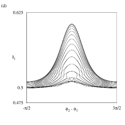
Figure 1: Phase portraits of system (8) composed of $N=3$ oscillators at parameter values $\beta=0$, $\varepsilon=0.39$, $\omega_{1}=-1$, $\omega_{2}=0$, $\omega_{3}=1$. (a) Phase portrait for fixed populations $I_{1}=I_{2}=I_{3}=1/2$ and initial phases for all trajectories $\phi_{2}-\phi_{1}=\pi-(\phi_{3}-\phi_{2})$. (b,c,d) Phase portraits for unfixed populations $I_{1}=I_{3}=1/2+0.01$, $I_{2}=1/2-0.02$, panel (b) shows dynamics of phase shifts, (c) shows evolution of populations of first and third oscillators, (d) illustrates dynamics of population of first oscillator vs. phase shift between first and second oscillators.

Following result requires clarification. At $\varepsilon=1$ trajectories on the two-dimensional invariant torus $I_{1}=I_{2}=I_{3}=1/2$ condense at $\phi_{2}-\phi_{1}=\phi_{3}-\phi_{2}=\pi/2$. At $\varepsilon>1$ points $\mathcal{O}_{1}$ and $\mathcal{O}_{2}$ appear which are effectively an attractor and a repeller of phase model (2) acting on the invariant torus $I_{1}=I_{2}=I_{3}=1/2$ of model (8) with fixed $\mathcal{H}=0$ and $C^{2}=3/2$. It is important to note that invariant torus $I_{1}=I_{2}=I_{3}=1/2$ at $\varepsilon>1$ is actually a stable manifold of saddle equilibrium $\mathcal{O}_{1}$ and unstable manifold of saddle equilibrium $\mathcal{O}_{2}$ in four-dimensional phase space. These two points are in involution with each other (and connected by heteroclinic trajectories) so we can discuss only one of them. Saddle equilibrium $\mathcal{O}_{1}$ has two-dimensional stable manifold (the invariant torus with fixed populations $I_{1}=I_{2}=I_{3}=1/2$) and two-dimensional unstable manifold. We illustrate this conclusion with calculation of Lyapunov exponents of Hamiltonian model (8) for trajectories with $I_{1}=I_{2}=I_{3}=1/2$. Fig. 2 demonstrates dependence of Lyapunov exponents from $\varepsilon$. At $\varepsilon<1$ all Lyapunov exponents are zero. This corresponds to periodic orbits on invariant torus. At $\varepsilon>1$ only two Lyapunov exponents are zero (since we have two constants of motion), and other four are two pairs of positive and negative exponents. This corresponds to two saddle equilibriums in involution. Stability of equilibrium $\mathcal{O}_{1}$ on invariant torus is compensated by instability in its neigborhood resulting in fast deviation of populations. In fact we can call states at $\varepsilon>1$ phase-locked and states at $\varepsilon<1$ amplitude-locked. We are confident that at $\varepsilon>1$ chaotic trajectories exist outside the invariant torus $I_{1}=I_{2}=I_{3}=1/2$ but we have troubles with their numerical demonstration. Observation of attractors and repellers in conservative system (8) with condition $I_{1}=I_{2}=I_{3}=1/2$ gives us reason to compare phase model (2) with nonholonomic mechanical system.

Figure 2: Lyapunov exponents vs. $\varepsilon$ on the invariant torus for $N=3$. $\beta=0$, $\omega_{1}=-1$, $\omega_{2}=0$, $\omega_{3}=1$.

To visualize dynamics of system (8) with more oscillators we need to construct suitable Poincaré cross-section. For the case of $N=4$ oscillators we follow [2] and choose cross-section by surface $\phi_{3}-\phi_{2}=\pi/2$ so that the invariant set of the involution is $\phi_{2}-\phi_{1}=\pi-(\phi_{4}-\phi_{3})$ on this surface.

First we discuss dynamics on the invariant torus $I_{j}=1/2$. It is three-dimensional in flow system (8) and two-dimensional in Poincaré cross-section. Fig. 3 demonstrates phase portraits in Poincaré cross-section of lattice (8) composed of $N=4$ oscillators. Populations $I_{1}=I_{2}=I_{3}=I_{4}=1/2$ are fixed and initial phases for all trajectories belong to the invariant set of involution. Parameters are $\beta=0$, $\omega_{1}=-1.5$, $\omega_{2}=-0.5$, $\omega_{3}=0.5$, $\omega_{4}=1.5$. For small coupling $\varepsilon=0.19$ dynamics on the invariant torus $I_{j}=1/2$ is quasiperiodic and measure-preserving. For larger coupling $\varepsilon=0.39$ invariant torus $I_{j}=1/2$ contains quasi-periodic and chaotic trajectories, but dynamics is still measure-preserving. At coupling $\varepsilon=0.49$ invariant torus $I_{j}=1/2$ has coexisting attractor $\mathcal{A}$ with its reversal repeller $\mathcal{R}$ and dynamics is no more measure-preserving. In Poincaré cross-section attractor $\mathcal{A}$ has one-dimensional unstable manifold and one-dimensional stable manifold and phase volume on the invariant torus is overall contracting. Nevertheless in the neigborhood of the invariant torus $I_{j}=1/2$ there are two directions of expansion and contraction that compensate contraction of phase volume on invariant torus. At $\varepsilon>0.6$ invariant torus $I_{j}=1/2$ has two stable and unstable periodic orbits $\mathcal{C}_{1}$ and $\mathcal{C}_{2}$ in involution. The stable orbit $\mathcal{C}_{1}$ has two-dimensional stable manifold in Poincaré cross-section.

Fig. 4 demonstrates dependence on $\varepsilon$ of Lyapunov exponents of Hamiltonian model (8) for trajectories with $I_{j}=1/2$. There are eight Lyapunov exponents, but four of them are always zero (if trajectory is not an equilibrium), two due to constants of motion and two due to invariance to arbitrary time shift along the trajectory (one perturbation vector is tangent to the reference phase trajectory) and to arbitrary phase shift. We distinguish four regions of $\varepsilon$. The first corresponds to quasiperiodic motions with all exponents equal to zero ($\varepsilon<0.36$ approximately). The second corresponds to coexistence of quasiperiodic and chaotic motions with one positive and one negative exponent for perturbations on the invariant torus and one positive and one negative exponent for perturbations outside the invariant torus ($\varepsilon<0.43$ according to [2]). All nonzero Lyapunov exponents are equal in magnitude. The third is the interval with chaotic attractors $\mathcal{A}$ and repellers $\mathcal{R}$ ($\varepsilon<0.6$) with one positive and one negative exponent on the invariant torus, nonequal in magnitude. For $\varepsilon>0.6$ there are periodic orbits $\mathcal{C}_{1}$ and $\mathcal{C}_{2}$. Periodic orbit $\mathcal{C}_{1}$ has two nonequal negative Lyapunov exponents on the invariant torus, and two nonequal positive Lyapunov exponents outside the invariant torus. Periodic orbit $\mathcal{C}_{2}$ is in involution with $\mathcal{C}_{1}$. One can compare dependence of Lyapunov exponents for the Hamiltonian system (8) with the dependence of Lyapunov exponents for the system (2) in [2], where exponents for perturbations outside the invariant torus are absent.

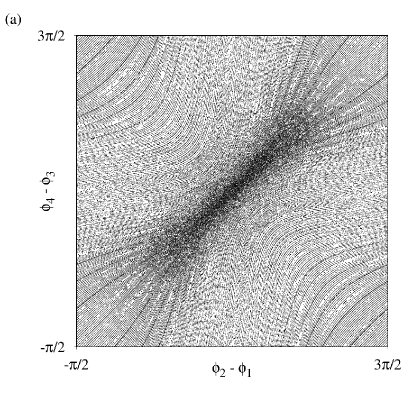
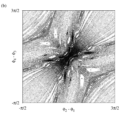
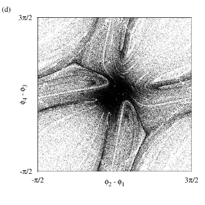
Figure 3: Phase portraits in Poincaré cross-section by surface $\phi_{3}-\phi_{2}=\pi/2$ of system (8) composed of $N=4$ oscillators. Populations $I_{1}=I_{2}=I_{3}=I_{4}=1/2$ are fixed and initial phases for all trajectories satisfy $\phi_{2}-\phi_{1}=\pi-(\phi_{4}-\phi_{3})$, $\phi_{3}-\phi_{2}=\pi/2$. Parameter values $\beta=0$, $\omega_{1}=-1.5$, $\omega_{2}=-0.5$, $\omega_{3}=0.5$, $\omega_{4}=1.5$. At $\varepsilon=0.19$ most of trajectories are regular (a). At $\varepsilon=0.39$ some of trajectories are chaotic, but attractors and repellers are absent (b). At $\varepsilon=0.49$ chaotic attractor and repeller coexist, panel (c) demonstrates evolution forward in time, panel (d) demonstrates evolution backward in time.

Figure 4: Lyapunov exponents vs. $\varepsilon$ on the invariant torus for $N=4$. $\beta=0$, $\omega_{1}=-1.5$, $\omega_{2}=-0.5$, $\omega_{3}=0.5$, $\omega_{4}=1.5$. Initial condition for all values of $\varepsilon$ was $I_{1}=I_{2}=I_{3}=I_{4}=1/2$, $\phi_{1}=-\pi/2$, $\phi_{2}=-\pi/3$, $\phi_{3}=\pi/6$, $\phi_{4}=\pi$. This initial condition belongs to the invariant set of involution.

Now we discuss motions outside the invariant torus $I_{j}=1/2$. Fig. 5 shows phase portrait in Poincaré cross-section of the lattice (8) composed of $N=4$ oscillators at coupling $\varepsilon=0.19$ with non-constant populations. Initial phases for all trajectories belong to the invariant set of involution. Dynamics is mostly quasiperiodic. Fig. 6 demonstrates phase portrait in Poincaré cross-section at coupling $\varepsilon=0.39$ with non-constant populations. We describe motions in neigborhood of the invariant torus following paper [7]. If phase shift between two neiboring oscillators becomes close to $\pi/2$, their populations unlock from vicinity of invariant torus $I_{j}\approx 1/2$ and grow fast and then return. These bursts occur along the unstable manifolds of saddle sets on the invariant torus, then trajectories return to vicinity of $I_{j}\approx 1/2$ along the stable manifolds of saddle sets on the invariant torus.

Fig. 4 shows dependence on $\varepsilon$ of Lyapunov exponents of Hamiltonian model (8) for trajectories with non-constant populations. If $\varepsilon>0.34$ four exponents become non-zero. Since dynamics is Hamiltonian, total sum of all Lyapunov exponents is zero.

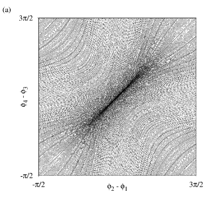
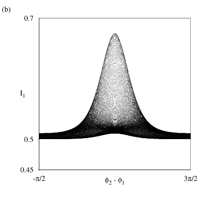
Figure 5: Phase portraits in Poincaré cross-section by surface $\phi_{3}-\phi_{2}=\pi/2$ of system (8) composed of $N=4$ oscillators. Populations are not fixed. Initial conditions for all trajectories satisfy $I_{1}=1/2+0.01$, $I_{2}=1/2-0.01$, $I_{3}=1/2-0.01$, $I_{4}=1/2+0.01$, $\phi_{2}-\phi_{1}=\pi-(\phi_{4}-\phi_{3})$, $\phi_{3}-\phi_{2}=\pi/2$. Parameter values $\varepsilon=0.19$, $\beta=0$, $\omega_{1}=-1.5$, $\omega_{2}=-0.5$, $\omega_{3}=0.5$, $\omega_{4}=1.5$. Panel (a) shows dynamics of phases, panel (b) shows population vs. phase shift.

Figure 6: Phase portraits in Poincaré cross-section by surface $\phi_{3}-\phi_{2}=\pi/2$ of system (8) composed of $N=4$ oscillators. Populations are not fixed. Initial conditions for all trajectories satisfy $I_{1}=1/2+0.01$, $I_{2}=1/2-0.01$, $I_{3}=1/2-0.01$, $I_{4}=1/2+0.01$, $\phi_{2}-\phi_{1}=\pi-(\phi_{4}-\phi_{3})$, $\phi_{3}-\phi_{2}=\pi/2$. Parameter values $\varepsilon=0.39$, $\beta=0$, $\omega_{1}=-1.5$, $\omega_{2}=-0.5$, $\omega_{3}=0.5$, $\omega_{4}=1.5$. Panel (a) shows dynamics of phases, panel (b) shows population vs. phase shift.

Figure 7: Lyapunov exponents vs. $\varepsilon$ for $N=4$ with non-constant populations. $\beta=0$, $\omega_{1}=-1.5$, $\omega_{2}=-0.5$, $\omega_{3}=0.5$, $\omega_{4}=1.5$. Initial condition for all values of $\varepsilon$ was $I_{1}=1/2+0.01$, $I_{2}=1/2-0.01$, $I_{3}=1/2-0.01$, $I_{4}=1/2+0.01$, $\phi_{1}=-\pi/2$, $\phi_{2}=-\pi/3$, $\phi_{3}=\pi/6$, $\phi_{4}=\pi$.

4 Dissipative models close to Topaj – Pikovsky system

We propose two dissipative models close to Topaj – Pikovsky system. The first is a lattice of dissipative pendulums with local coupling:

$$m\ddot{\psi}_{j}+\dot{\psi}_{j}=1+\varepsilon\sin\psi_{j+1}+\varepsilon\sin\psi_{j-1}-2\varepsilon\sin\psi_{j},$$ (12)

If we set masses $m=0$, then the system (12) becomes the Topaj – Pikovsky model. Model (12) with non-zero masses is not reversible. Terms with second derivatives destroy “fat” attractor [8] of Topaj – Pikovsky system. If masses are small, then transient trajectories appear similar to Topaj – Pikovsky phase portraits at short times of evolution.

The second model is a lattice of locally coupled amplitude-phase equations derived from van der Pol equations:

$$\dot{\alpha}_{j} =\frac{1}{2}\left(\lambda-\alpha_{j}^{2}\right)\alpha_{j}-$$ (13)

$$-\varepsilon\left(\alpha_{j}-\alpha_{j-1}\cos{\left(\phi_{j-1}-\phi_{j}\right)}\right)-\varepsilon\left(\alpha_{j}-\alpha_{j+1}\cos{\left(\phi_{j+1}-\phi_{j}\right)}\right),$$

$$\dot{\phi}_{j} =\omega_{j}+\varepsilon\frac{\alpha_{j-1}}{\alpha_{j}}\sin{\left(\phi_{j-1}-\phi_{j}\right)}+\varepsilon\frac{\alpha_{j+1}}{\alpha_{j}}\sin{\left(\phi_{j+1}-\phi_{j}\right)},$$

with $\omega_{j+1}-\omega_{j}=1$.

If amplitudes $\alpha_{j}$ are close to constant: $\alpha_{j}=\sqrt{\lambda}\left(1+r_{j}\right)$, $r_{j}\ll 1$ then we derive

$$\dot{r}_{j} =-\lambda r_{j}+\varepsilon\left(\cos{\left(\phi_{j-1}-\phi_{j}\right)}-1\right)+\varepsilon\left(\cos{\left(\phi_{j+1}-\phi_{j}\right)}-1\right),$$ (14)

$$\dot{\phi}_{j} =\omega_{j}+\varepsilon\left(1+r_{j-1}-r_{j}\right)\sin{\left(\phi_{j-1}-\phi_{j}\right)}+\varepsilon\left(1+r_{j+1}-r_{j}\right)\sin{\left(\phi_{j+1}-\phi_{j}\right)}.$$

Now we can reduce dimension of system (14) $\rho_{j}=r_{j+1}-r_{j}$, $\psi_{j}=\phi_{j+1}-\phi_{j}$:

$$\dot{\rho}_{j} =-\lambda\rho_{j}+\varepsilon\cos{\psi_{j+1}}-\varepsilon\cos{\psi_{j-1}},$$ (15)

$$\dot{\psi}_{j} =\Delta_{j}+\varepsilon\left(1+\rho_{j+1}\right)\sin{\psi_{j+1}}+\varepsilon\left(1-\rho_{j-1}\right)\sin{\psi_{j-1}}-2\varepsilon\sin{\psi_{j}}.$$

System (15) is close to Topaj – Pikovsky model but not reversible.

5 Conclusion

We discussed Hamiltonian model of oscillator lattice that describes spatial modes of one-dimensional Bose – Einstein condensate in tilted optical lattice. Phase space of Hamiltonian model has invariant manifolds with dynamics governed exactly by Topaj – Pikovsky equations. System is reversible with involution similar to Topaj – Pikovsky model. We suppose this model deserves further studying. There are promising connections with phenomenon of synchronization [7, 9, 10], nonholonomic mechanics and integrability.

Funding

Russian Science Foundation, project No. 15-12-20035.

References

• [1]
• [2] Topaj, D. and Pikovsky, A., Reversibility vs. synchronization in oscillator lattices, Physica D: Nonlinear Phenomena, 2002, vol. 170, no. 2, pp. 118–130.
• [3] Gonchenko, A. S., Gonchenko, S. V., Kazakov, A. O. and Turaev, D. V., On the phenomenon of mixed dynamics in Pikovsky – Topaj system of coupled rotators, Physica D: Nonlinear Phenomena, 2017, vol. 350, pp. 45–57.
• [4] Roberts, J. A. G. and Quispel, G. R. W., Chaos and time-reversal symmetry. Order and chaos in reversible dynamical systems, Physics Reports, 1992, vol. 216, no. 2-3, pp. 63–177.
• [5] Borisov, A. V. and Mamaev, I. S., Strange attractors in rattleback dynamics, Physics-Uspekhi, 2003, vol. 46, no. 4. pp. 393.
• [6] Thommen, Q., Garreau, J. C. and Zehnlé, V., Classical chaos with Bose-Einstein condensates in tilted optical lattices, Physical review letters, 2003, vol. 91, no. 21, pp. 210405.
• [7] Witthaut, D. and Timme, M., Kuramoto dynamics in Hamiltonian systems Physical Review E., 2014, vol. 90, no. 3, pp. 032917.
• [8] Bizyaev, I. A., Borisov, A. V. and Kuznetsov S. P, The Chaplygin sleigh with friction moving due to periodic oscillations of an internal mass, Nonlinear Dynamics, 2018, vol. 95, no. 1, pp. 699–714.
• [9] Hampton, A. and Zanette, D. H., Measure synchronization in coupled Hamiltonian systems, Physical review letters, 1999, vol. 83, no. 11, pp. 2179.
• [10] Vincent, U. E., Njah, A. N. and Akinlade, O., Measure synchronization in a coupled Hamiltonian system associated with Nonlinear Schrödinger Equation, Modern Physics Letters B. 2005, vol. 19, no. 15, pp. 737–742.