Bounce Configuration from Gradient Flow

Abstract

Based on the gradient flow, we propose a new method to determine the bounce configuration for false vacuum decay. Our method is applicable to a large class of models with multiple fields. Since the bounce is a saddle point of an action, a naive gradient flow method which minimizes the action does not work. We point out that a simple modification of the flow equation can make the bounce its stable fixed point while the false vacuum configuration an unstable one. Consequently, the bounce configuration can be obtained simply by following the flow without a careful choice of an initial configuration. With numerical analysis, we confirm the validity of our claim, checking that the flow equation we propose indeed has solutions that flow into the bounce configuration.

Introduction: Study of false vacua (and metastable states) has been important in various fields, like particle physics, cosmology, nuclear physics, condensed matter physics, and so on. For example, in the field of particle physics and cosmology, the stability of the electroweak vacuum has been attracted much attention. In particular, taking the best-fit values of the observed top-quark and Higgs-boson masses, and assuming that the standard model of particle physics is valid up to a very high scale (like the Planck scale), the electroweak vacuum is metastable Isidori:2001bm ; Degrassi:2012ry . It is because the Higgs quartic coupling constant becomes negative at a high energy scale due to the renormalization group effects. Performing precise calculation based on relativistic quantum field theory, the decay rate of the electroweak vacuum per unit volume is known to be $\sim 10^{-582}\ {\rm Gyr^{-1}Gpc^{-3}}$ Chigusa:2017dux ; Chigusa:2018uuj ; Andreassen:2017rzq , with which the stability of our universe looks plausible for the present cosmic time scale. However, this conclusion may be altered with the introduction of new physics beyond the standard model. The studies of the stability of the electroweak vacuum in such new physics models remain important.

In relativistic quantum field theory, the decay of the false vacuum is mainly induced by the field configuration called “bounce” Coleman:1977py ; Callan:1977pt ; Coleman:aspectsof . Bounce is a configuration obeying the classical equation of motion (EOM) derived from the Euclidean action. With the bounce, which we denote as $\bar{\phi}$, the decay rate of the false vacuum per unit volume is given in the following form:

$$\gamma={\cal A}e^{-{\cal S}[\bar{\phi}]},$$ (1)

where ${\cal S}[\bar{\phi}]$ is the bounce action while ${\cal A}$ is a prefactor. The decay rate is highly sensitive to the bounce action so that the profile of the bounce should be well understood for an accurate calculation of the decay rate.

In spite of the importance of determining the bounce configuration with a generic potential, it is not easy in general. The difficulty mainly comes from the fact that the bounce is a saddle point, not a minimum, of the action. Consequently, the fluctuation matrix around the bounce has a negative eigenvalue and a small fluctuation destabilizes the bounce. Although there have been many attempts to find methods to determine the bounce configuration with overcoming this difficulty Claudson:1983et ; Kusenko:1995jv ; Kusenko:1996jn ; Dasgupta:1996qu ; Moreno:1998bq ; John:1998ip ; Cline:1998rc ; Cline:1999wi ; Konstandin:2006nd ; Wainwright:2011kj ; Akula:2016gpl ; Masoumi:2016wot ; Espinosa:2018hue ; Jinno:2018dek ; Espinosa:2018szu ; Athron:2019nbd , new ideas are still awaited for a detailed understanding of the bounce as well as for a precise calculation of its configuration via numerical analysis.

In this letter, we propose a new method to determine the bounce configuration, where we use the gradient flow method. It does not work if we naively use the action, ${\cal S}$, to calculate the gradient in the configuration space. The failure of the naive method is due to the negative eigenvalue mode as we have mentioned. We discuss that, with a simple modification of the flow equation, the bounce configuration can become a stable fixed point while it makes the false vacuum and other stable solutions of the classical EOM unstable. We also show that, with numerical analysis, the bounce configuration can be obtained by solving the flow equation we propose.

Formulation: We adopt the action in the following form:

$${\cal S}[\phi]=\int d^{D}x\left[\frac{1}{2}\partial_{\mu}\phi_{A}\partial_{\mu}\phi_{A}+V(\phi)\right],$$ (2)

where $D$ is the dimension of the Euclidean space, $\phi_{A}$ denotes a real scalar field (with $A$ being flavor index), and $V$ is the scalar potential. Because the bounce is a spherical object Coleman:1977th ; Blum:2016ipp , $\phi_{A}$ depends only on the radial coordinate of the Euclidean space, $r$, and obeys the following classical EOM:

$$\left.\frac{\delta{\cal S}[\phi]}{\delta\phi_{A}}\right|_{\phi\rightarrow\bar{\phi}}=-\partial_{r}^{2}\bar{\phi}_{A}-\frac{D-1}{r}\partial_{r}\bar{\phi}_{A}+\left.\frac{\partial V}{\partial\phi_{A}}\right|_{\phi\rightarrow\bar{\phi}}=0,$$ (3)

satisfying the following boundary conditions:

$$\partial_{r}\bar{\phi}_{A}(r=0)=0,~{}~{}~{}\bar{\phi}_{A}(r\rightarrow\infty)=v_{A},$$ (4)

where $v_{A}$ is the field amplitude of the $A$-th scalar field at the false vacuum. In the following, we explain how we obtain the bounce configuration.

Before going into the details, we introduce the fluctuation operator, which plays important roles in our discussion. In $D$-dimensional Euclidean space, the fluctuation operator around the bounce is given by

$${\cal M}_{AB}\equiv-\left(\partial_{r}^{2}+\frac{D-1}{r}\partial_{r}\right)\delta_{AB}+\left.\frac{\partial^{2}V}{\partial\phi_{A}\partial\phi_{B}}\right|_{\phi\rightarrow\bar{\phi}}.$$ (5)

Spherical fluctuations around the bounce can be expressed as linear combinations of the eigenfunctions of ${\cal M}_{AB}$. We denote eigenfunctions of ${\cal M}_{AB}$ as $\chi_{n,A}$ ($n=-1$, $1$, $2$, $\cdots$), i.e.,

$${\cal M}_{AB}\chi_{n,B}=\lambda_{n}\chi_{n,A},$$ (6)

where $\lambda_{n}$ is the eigenvalue. The eigenfunctions should satisfy the following boundary conditions:

$$\partial_{r}\chi_{n,A}(r=0)=0,~{}~{}~{}\chi_{n,A}(r\rightarrow\infty)=0,$$ (7)

and are normalized as

$$\langle\chi_{n}|\chi_{n^{\prime}}\rangle=\delta_{nn^{\prime}},$$ (8)

where the inner product of two sets of functions is defined as

$$\langle f|f^{\prime}\rangle\equiv\int_{0}^{\infty}drr^{D-1}f_{A}(r)f^{\prime}_{A}(r).$$ (9)

An important property of the bounce is that the fluctuation operator around the bounce has one negative eigenvalue Callan:1977pt , which we call $\lambda_{-1}<0$. We also assume that all the other eigenvalues are positive.

Hereafter, we discuss a method in which a function $\Phi_{A}(r,s)$, with $s$ being the “flow time,” evolves to the bounce configuration as $s\rightarrow\infty$. The initial profile $\Phi_{A}(r,s=0)$ is required to satisfy the boundary conditions same as the bounce (see (4)). Then, the boundary conditions are kept during the flow by the flow equation introduced below. In other words, $\Phi_{A}(r,s)-\bar{\phi}_{A}$ stays in the configuration space spanned by the eigenfunctions of ${\cal M}_{AB}$, and hence $\Phi_{A}(r,s)$ can be expressed as

$$\Phi_{A}(r,s)=\bar{\phi}_{A}(r)+\sum_{n}a_{n}(s)\chi_{n,A}(r).$$ (10)

To obtain the bounce configuration using a flow equation, we need to flip the sign of the negative eigenvalue around the bounce. The flow equation we propose is as follows:

$$\partial_{s}\Phi_{A}(r,s)=F_{A}(r,s)-\beta\langle F|g\rangle g_{A}(r),$$ (11)

where $\beta$ is a dimensionless constant. Here, $g_{A}$ is a function satisfying the same boundary conditions as $\chi_{n,A}$ (see Eq. (7)), and is normalized as

$$\langle g|g\rangle=1.$$ (12)

We expand $g_{A}$ as

$$g_{A}(r)=\sum_{n}c_{n}\chi_{n,A}(r),$$ (13)

where $\sum_{n}c_{n}^{2}=1$. In addition,

$$F_{A}\equiv-\frac{\delta{\cal S}[\Phi]}{\delta\Phi_{A}}=\partial_{r}^{2}\Phi_{A}+\frac{D-1}{r}\partial_{r}\Phi_{A}-\frac{\partial V(\Phi)}{\partial\Phi_{A}}.$$ (14)

Notice that $F_{A}$ satisfies the same boundary conditions as $\chi_{n,A}$ as far as $\Phi_{A}$ is in the form of Eq. (10), guaranteeing that $\Phi_{A}$ is expressed as in Eq. (10) for any value of $s$. As we will see in the following, the second term in the right-hand side of Eq. (11) can make the bounce configuration a stable fixed point.

Importantly, for $\beta\neq 1$, any fixed point solution of Eq. (11), which satisfies $\partial_{s}\Phi_{A}=0$, is a solution of the classical EOM, $F_{A}=0$. This can be understood by using the following relation:

$$\langle\partial_{s}\Phi|g\rangle=(1-\beta)\langle F|g\rangle.$$ (15)

If $\partial_{s}\Phi_{A}=0$ is realized with non-vanishing $F_{A}$, $F_{A}$ and $g_{A}$ should be proportional to each other to satisfy the flow equation. Such a requirement contradicts with Eq. (15) because the left-hand side of Eq. (15) vanishes while the right-hand side does not. It also implies that the flow equation of our proposal does not have any unwanted fixed point that does not correspond to a solution of the classical EOM.

Now, we show that, with properly choosing $\beta$ and $g_{A}$, the flow equation (11) has solutions that evolve to the bounce as $s\rightarrow\infty$. For this purpose, we analyze the flow around the bounce configuration, where $a_{n}$ can be treated as a small quantity. Keeping terms linear in $a_{n}$, we obtain

$$F_{A}\simeq-{\cal M}_{AB}(\Phi_{B}-\bar{\phi}_{B})=-\sum_{n}\lambda_{n}a_{n}\chi_{n,A},$$ (16)

which gives $\langle F|g\rangle\simeq-\sum_{n}\lambda_{n}c_{n}a_{n}$. Thus, the flow equation gives

$$\dot{a}_{n}\simeq-\lambda_{n}a_{n}+\beta\sum_{m}c_{n}c_{m}\lambda_{m}a_{m}\equiv-\sum_{m}\Gamma_{nm}(\beta)a_{m},$$ (17)

where the “dot” is the derivative with respect to $s$.

If we consider the naive flow equation which minimizes the action (i.e. the case with $\beta=0$), we obtain $\dot{a}_{n}\simeq-\lambda_{n}a_{n}$. Then, the coefficient of the mode with the negative eigenvalue $\lambda_{-1}$ grows with flow time. This is the reason why the naive gradient flow method does not work to find the bounce.

With a non-vanishing value of $\beta$, the above conclusion may change. To see this, we express $\Gamma(\beta)$ in Eq. (17) in the matrix form:

$$\Gamma(\beta)=\left({\rm I}-\beta\vec{c}\,\vec{c}^{\,T}\right)\mbox{diag}(\lambda_{-1},\lambda_{1},\lambda_{2},\cdots),$$ (18)

where ${\rm I}$ is the unit matrix, the superscript, $T$, denotes the transpose, and

$$\vec{c}=(c_{-1},c_{1},c_{2},\cdots)^{\,T}.$$ (19)

If the real parts of all the eigenvalues of $\Gamma$ are positive, $\Phi_{A}(r,s\rightarrow\infty)=\bar{\phi}_{A}(r)$ is realized. Notice that $\vec{c}$ is an eigenvector of the matrix $({\rm I}-\beta\vec{c}\,\vec{c}^{\,T})$ with the eigenvalue of $(1-\beta)$. In addition, all the other eigenvalues are $1$ because $({\rm I}-\beta\vec{c}\,\vec{c}^{\,T})\vec{v}_{\perp}=\vec{v}_{\perp}$ if $\vec{c}^{\,T}\vec{v}_{\perp}=0$. Thus, we have

$$\mbox{det}\left({\rm I}-\beta\vec{c}\,\vec{c}^{\,T}\right)=1-\beta,$$ (20)

and hence

$$\mbox{det}\Gamma(\beta)=(1-\beta)\prod_{n}\lambda_{n}.$$ (21)

For $\beta>1$, $\mbox{det}\Gamma>0$ (because $\prod_{n}\lambda_{n}<0$), which opens a possibility to make the real parts of all the eigenvalues of $\Gamma(\beta>1)$ positive.

The evolution of $\vec{a}\equiv(a_{-1},a_{1},a_{2},\cdots)^{T}$ is complicated in general because $\Gamma$ is not symmetric. If we consider the condition $\partial_{s}(\vec{a}^{\,T}\vec{a})<0$, which is a sufficient condition for the bounce to be a stable fixed point, the discussion becomes simpler; it requires $\Gamma+\Gamma^{T}$ to be positive definite. In order for $\Gamma(\beta>1)+\Gamma^{T}(\beta>1)$ to be positive definite, $\vec{c}^{\,T}[\Gamma(\beta>1)+\Gamma^{T}(\beta>1)]\vec{c}>0$ should hold, and hence

$$\langle g|{\cal M}g\rangle=\sum_{n}\lambda_{n}c_{n}^{2}<0,$$ (22)

which gives a guideline in choosing the function, $g_{A}$. In addition, because the smallest eigenvalue of $\Gamma+\Gamma^{T}$ is smaller than its smallest diagonal element, $\beta$ should be in the following range:

$$\frac{1}{c_{-1}^{2}}<\beta<\frac{1}{\mbox{max}_{n\geq 1}c_{n}^{2}}.$$ (23)

We can see that a choice of $g_{A}$ with larger $|c_{-1}|$ and smaller $|c_{n\geq 1}|$ is better though their exact values are unknown until the bounce is obtained. We will discuss the choice of $g_{A}$ later.

Let us summarize the properties of the flow equation of Eq. (11). If $\Phi_{A}(r,s\rightarrow\infty)$ converges with $\beta>1$, it is guaranteed that (i) $\Phi_{A}(r,s\rightarrow\infty)$ is a solution of the classical EOM, (ii) $\Phi_{A}(r,s\rightarrow\infty)$ satisfies the boundary conditions relevant for the bounce, and (iii) the fluctuation operator around $\Phi_{A}(r,s\rightarrow\infty)$ has one negative eigenvalue. The statement (iii) is due to the fact that the real parts of all the eigenvalues of $\Gamma(\beta>1)$ should be positive to make $\Phi_{A}(r,s\rightarrow\infty)$ stable against fluctuations, which implies that $\Gamma(\beta=0)$ has one negative eigenvalue assuming that there is no degeneracy in the eigenvalues of $\Gamma(\beta=1)$. Thus, $\Phi_{A}(r,s\rightarrow\infty)$ obtained with $\beta>1$ is expected to be the bounce configuration. We also emphasize that, because of (iii), all the stable fixed points for $\Gamma(\beta=0)$ are destabilized. Thus, for example, the resultant configuration $\Phi_{A}(r,s\rightarrow\infty)$ cannot be the false vacuum configuration when $\beta>1$.

Numerical Analysis: So far, we have studied the behavior of the fluctuations around the bounce and have seen that the bounce configuration can become a fixed point of the flow equation. In the following, by using numerical calculations, we explicitly show that there exist solutions that indeed flow to the bounce configuration.

To perform numerical calculations, the function $g_{A}$ should be fixed. We take

$$g_{A}\propto r\partial_{r}\Phi_{A},$$ (24)

which is based on the following consideration. Since we have

$$\int_{0}^{\infty}drr^{D-1}(r\partial_{r}\bar{\phi}_{A}){\cal M}_{AB}(r\partial_{r}\bar{\phi}_{B})$$

$$=-(D-2)\int_{0}^{\infty}drr^{D-1}(\partial_{r}\bar{\phi}_{A})(\partial_{r}\bar{\phi}_{A}),$$ (25)

the condition (22) is satisfied for $D>2$. It implies that $g_{A}$ of our choice has a large $|c_{-1}|$. In addition, it satisfies the relevant boundary conditions.

To solve Eq. (11), we discretize the radius coordinate, $r$, and solve the ordinary differential equations with respect to $s$. To impose the boundary conditions of Eq. (4), it is better to shrink $r\in(0,\infty)$ into $x\in(0,1)$ with

$$x=\tanh\left(\frac{r}{R}\right),$$ (26)

and attach the endpoints, $x=0$ and $x=1$. In our analysis, $R$ is taken to the size of the bounce. Then, we discretize $x$ into $N+1$ lattice points:

$$x_{0}=0,~{}x_{1}=\frac{1}{N},~{}x_{2}=\frac{2}{N},\cdots,~{}x_{N}=1.$$ (27)

The flow equation in terms of $x$ is given by

$$\partial_{\sigma}\hat{\Phi}_{A}(x,\sigma)=2\sigma(1-x^{2})\left[\hat{F}_{A}(x,\sigma)-\beta\frac{\langle\hat{F}|\hat{g}\rangle_{x}}{\langle\hat{g}|\hat{g}\rangle_{x}}\hat{g}_{A}(x,\sigma)\right],$$ (28)

where $\sigma=s^{1/2}/R$,

$$\hat{\Phi}_{A}(x,\sigma) =R^{\frac{D}{2}-1}\Phi_{A}(R{\,\rm arctanh}(x),R^{2}\sigma^{2}),$$ (29)

$$\hat{g}_{A}(x,\sigma) ={\,\rm arctanh}(x)\partial_{x}\hat{\Phi}_{A}(x,\sigma),$$ (30)

and

$$\hat{F}_{A}= \,(1-x^{2})\partial_{x}^{2}\hat{\Phi}_{A}+\frac{D-1-2x{\,\rm arctanh}(x)}{{\,\rm arctanh}(x)}\partial_{x}\hat{\Phi}_{A}$$

$$\,-\frac{R^{\frac{D}{2}+1}}{1-x^{2}}\frac{\partial V}{\partial\phi_{A}}.$$ (31)

Furthermore, the inner product is defined as

$$\langle\hat{f}|\hat{f}^{\prime}\rangle_{x}\equiv\int_{0}^{1}dx(1-x^{2}){\,\rm arctanh}^{D-1}(x)\hat{f}_{A}(x)\hat{f}^{\prime}_{A}(x).$$ (32)

Here, we adopt the second-order central differences for the derivatives with respect to $x$.

In numerically solving the flow equation, we take the following initial configuration of $\hat{\Phi}_{A}$:

$$\hat{\Phi}_{A}(x_{n},0)=R^{\frac{D}{2}-1}[w_{A}+x_{n}^{2}(v_{A}-w_{A})],$$ (33)

where $w_{A}=\Phi_{A}(x_{0},0)$ is a constant; $\Phi_{A}(x_{0},0)$ is set to be somewhere near the true vacuum (see figures). At each step of the flow, $\hat{\Phi}_{A}(x_{1},\sigma),\cdots,\hat{\Phi}_{A}(x_{N-1},\sigma)$ are determined by Eq. (28), while the endpoint values are fixed by the boundary conditions:

$$\hat{\Phi}_{A}(x_{0},\sigma)=\frac{4\hat{\Phi}_{A}(x_{1},\sigma)-\hat{\Phi}_{A}(x_{2},\sigma)}{3},$$ (34)

$$\hat{\Phi}_{A}(x_{N},\sigma)=R^{\frac{D}{2}-1}v_{A}.$$ (35)

Notice that Eq. (34) is equivalent to $\partial_{r}\Phi_{A}=0$ at $r=0$ (where we used $\partial_{x}\hat{\Phi}_{A}(x_{0},\sigma)\simeq\partial_{x}\hat{\Phi}_{A}(x_{1},\sigma)-\partial_{x}^{2}\hat{\Phi}_{A}(x_{1},\sigma)/N$), while Eq. (35) guarantees $\Phi_{A}(r=\infty)=v_{A}$. After the convergence of $\hat{\Phi}_{A}$, we calculate the bounce action. With the use of the equation of motion for the bounce, the action is calculated as

$${\cal S}[\bar{\phi}]=\frac{S_{D-1}}{D}\langle\partial_{x}\hat{\Phi}|\partial_{x}\hat{\Phi}\rangle_{x},$$ (36)

where $S_{D-1}$ is the surface area of the $(D-1)$-dimensional sphere.

Here, we take $D=3$, and use the following benchmark potentials for single- and double-scalar cases:

$$V^{\rm(single)} =\frac{1}{4}\phi^{4}-\frac{k_{1}+1}{3}\phi^{3}+\frac{k_{1}}{2}\phi^{2},$$ (37)

$$V^{\rm(double)} =\left(\phi_{x}^{2}+5\phi_{y}^{2}\right)\left[5(\phi_{x}-1)^{2}+(\phi_{y}-1)^{2}\right]$$

$$\hskip 12.91663pt+k_{2}\left(\frac{1}{4}\phi_{y}^{4}-\frac{1}{3}\phi_{y}^{3}\right),$$ (38)

with $k_{1}$ and $k_{2}$ being constants. With our choices of parameters, the false and true vacua of $V^{\rm(single)}$ ($V^{\rm(double)}$) are $\phi=0$ and $1$ ($(\phi_{x},\phi_{y})=(0,0)$ and $(1,1)$), respectively. For the single-scalar (double-scalar) case, we take $k_{1}=0.47$ and $0.2$ ($k_{2}=2$ and $80$), which correspond to the thin-walled and thick-walled bounces, respectively.

We emphasize that the initial configurations, the model parameters, $\beta$, and the other lattice parameters are not special choices. We checked that the bounce can be obtained as a result of flow with generic choices of parameters.

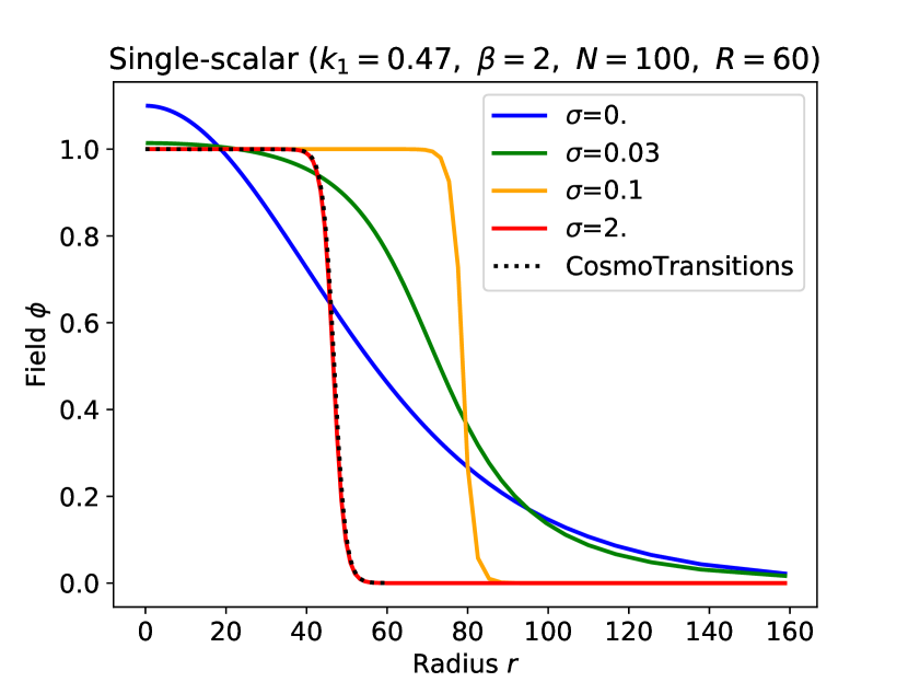
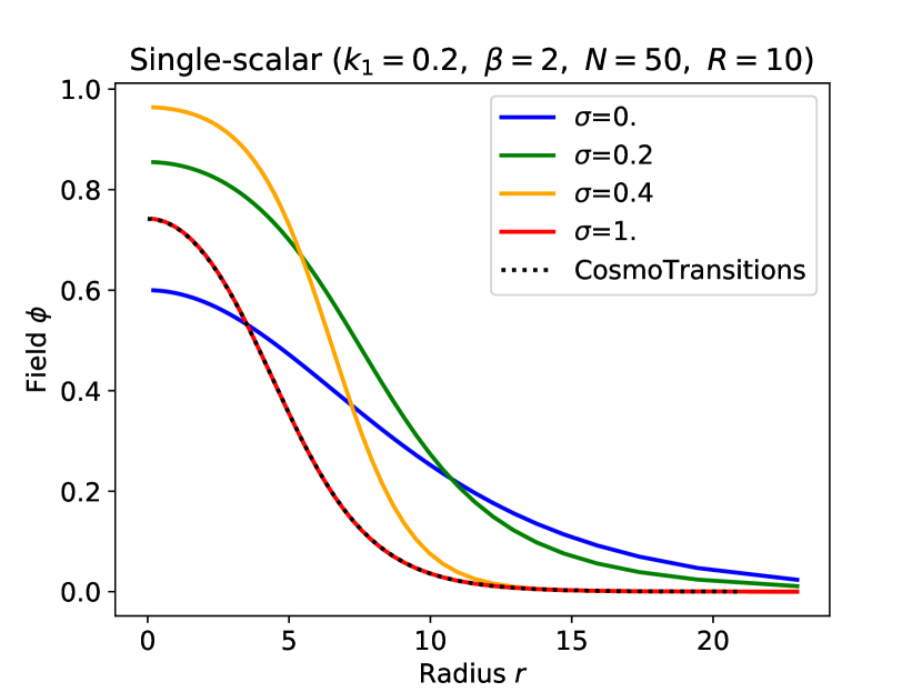
Figure 1: The flow of $\Phi$ for the single-scalar potential. The configuration is shown with the solid line for each $\sigma$. The results of CosmoTransitions are also shown with dotted lines. The parameters are shown on the top of each panel.

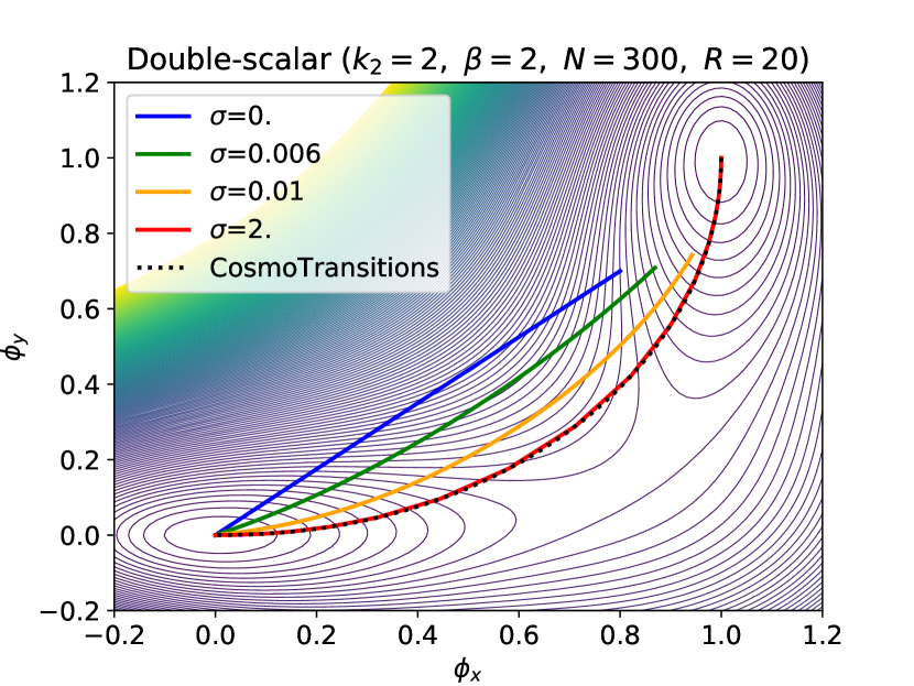
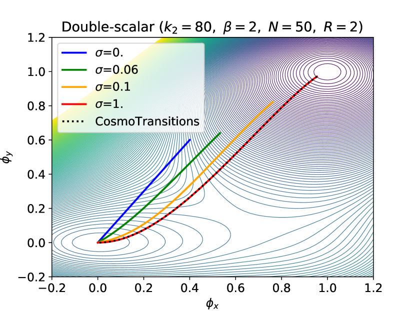
Figure 2: The flow of $\Phi$ for the double-scalar potential. The configuration is shown with the solid line for each $\sigma$. The results of CosmoTransitions are also shown with dotted lines. The parameters are shown on the top of each panel. We also show the contours of constant $V^{\rm(double)}$.

The flows of $\Phi_{A}$ based on our method are shown in Figs. 1 (for the single-scalar potential) and 2 (for the double-scalar potential) with the solid lines. In each figure, the solid line with the largest $\sigma$ shows the field configuration after the convergence; we checked that the flow after such an epoch is negligible. For comparison, we also determine the bounces for the same models by using CosmoTransitions Wainwright:2011kj , which are shown with the dotted lines. (We use the default control parameters of CosmoTransitions except for fRatioConv=0.001, which improves the accuracy in the multi-field calculation.) In addition, we calculate the bounce action ${\cal S}[\bar{\phi}]$ for each case:

$$\mathcal{S}^{\rm(single)}_{k_{1}=0.47}[\bar{\phi}] =\begin{cases}1086.6,&{\rm Our~{}result},\\ 1092.8,&{\tt CosmoTransitions},\end{cases}$$ (39)

$$\mathcal{S}^{\rm(single)}_{k_{1}=0.2}[\bar{\phi}] =\begin{cases}6.6360,&{\rm Our~{}result},\\ 6.6490,&{\tt CosmoTransitions},\end{cases}$$ (40)

$$\mathcal{S}^{\rm(double)}_{k_{2}=2}[\bar{\phi}] =\begin{cases}1763.7,&{\rm Our~{}result},\\ 1767.7,&{\tt CosmoTransitions},\end{cases}$$ (41)

$$\mathcal{S}^{\rm(double)}_{k_{2}=80}[\bar{\phi}] =\begin{cases}4.4585,&{\rm Our~{}result},\\ 4.4661,&{\tt CosmoTransitions}.\end{cases}$$ (42)

As we can see from the figures and the values of $\mathcal{S}[\bar{\phi}]$, our results well agree with those of CosmoTransitions. This strongly suggests the validity of our gradient flow method to determine the bounce configuration.

Summary: In this letter, we have proposed a new method to determine the bounce configuration. We have pointed out that the bounce configuration can be a stable solution of the flow equation given in Eq. (11). If the solution of the flow equation evolves to a fixed configuration for $\beta>1$, the resultant configuration is always a saddle point of the action, i.e., the bounce configuration. We have analytically shown that the negative eigenvalue mode, which destabilizes the bounce configuration, can be made harmless and that the bounce configuration can become a stable solution of the flow equation. We have verified our claims by numerical analysis. We believe that our method of finding the bounce configuration is simple, powerful, and useful in many cases. It can be used in multi-scalar cases and can easily be implemented to numerical code. We also comment that, even though we have concentrated on the bounce, our method is applicable to a generic problem to find a saddle point in a configuration space.

Acknowledgements: This work was supported by JSPS KAKENHI Grant (Nos. 17J00813 [SC], 16H06490 [TM], 18K03608 [TM], and 16H06492 [YS]).

References

- (1)
- (2) G. Isidori, G. Ridolfi and A. Strumia, Nucl. Phys. B 609 (2001) 387 [hep-ph/0104016].
- (3) G. Degrassi, S. Di Vita, J. Elias-Miro, J. R. Espinosa, G. F. Giudice, G. Isidori and A. Strumia, JHEP 1208 (2012) 098 [arXiv:1205.6497 [hep-ph]].
- (4) S. Chigusa, T. Moroi and Y. Shoji, Phys. Rev. Lett. 119 (2017) no.21, 211801 [arXiv:1707.09301 [hep-ph]].
- (5) S. Chigusa, T. Moroi and Y. Shoji, Phys. Rev. D 97 (2018) no.11, 116012 [arXiv:1803.03902 [hep-ph]].
- (6) A. Andreassen, W. Frost and M. D. Schwartz, Phys. Rev. D 97 (2018) no.5, 056006 [arXiv:1707.08124 [hep-ph]].
- (7) S. R. Coleman, Phys. Rev. D 15 (1977) 2929; Erratum: [Phys. Rev. D 16 (1977) 1248].
- (8) C. G. Callan, Jr. and S. R. Coleman, Phys. Rev. D 16 (1977) 1762.
- (9) S. Coleman, “Aspects of Symmetry,” Cambridge University Press (1985) 265.
- (10) M. Claudson, L. J. Hall and I. Hinchliffe, Nucl. Phys. B 228 (1983) 501.
- (11) A. Kusenko, Phys. Lett. B 358 (1995) 51 [hep-ph/9504418].
- (12) A. Kusenko, P. Langacker and G. Segre, Phys. Rev. D 54 (1996) 5824 [hep-ph/9602414].
- (13) I. Dasgupta, Phys. Lett. B 394 (1997) 116 [hep-ph/9610403].
- (14) J. M. Moreno, M. Quiros and M. Seco, Nucl. Phys. B 526 (1998) 489 [hep-ph/9801272].
- (15) P. John, Phys. Lett. B 452 (1999) 221 [hep-ph/9810499].
- (16) J. M. Cline, J. R. Espinosa, G. D. Moore and A. Riotto, Phys. Rev. D 59 (1999) 065014 [hep-ph/9810261].
- (17) J. M. Cline, G. D. Moore and G. Servant, Phys. Rev. D 60 (1999) 105035 [hep-ph/9902220].
- (18) T. Konstandin and S. J. Huber, JCAP 0606 (2006) 021 [hep-ph/0603081].
- (19) C. L. Wainwright, Comput. Phys. Commun. 183 (2012) 2006 [arXiv:1109.4189 [hep-ph]].
- (20) S. Akula, C. Balázs and G. A. White, Eur. Phys. J. C 76 (2016) no.12, 681 [arXiv:1608.00008 [hep-ph]].
- (21) A. Masoumi, K. D. Olum and B. Shlaer, JCAP 1701 (2017) no.01, 051 [arXiv:1610.06594 [gr-qc]].
- (22) J. R. Espinosa, JCAP 1807 (2018) no.07, 036 [arXiv:1805.03680 [hep-th]].
- (23) R. Jinno, arXiv:1805.12153 [hep-th].
- (24) J. R. Espinosa and T. Konstandin, JCAP 1901 (2019) no.01, 051 [arXiv:1811.09185 [hep-th]].
- (25) P. Athron, C. Balázs, M. Bardsley, A. Fowlie, D. Harries and G. White, arXiv:1901.03714 [hep-ph].
- (26) S. R. Coleman, V. Glaser and A. Martin, Commun. Math. Phys. 58 (1978) 211.
- (27) K. Blum, M. Honda, R. Sato, M. Takimoto and K. Tobioka, JHEP 1705 (2017) 109 Erratum: [JHEP 1706 (2017) 060] [arXiv:1611.04570 [hep-th]].