A crossinggram for random fields on lattices

Abstract

The modeling of risk situations that occur in a space-time framework can be done using max-stable random fields on lattices. Although the summary coefficients for the spatial and temporal behaviour do not characterize the finite-dimensional distributions of the random field, they have the advantage of being immediate to interpret and easier to estimate. The coefficients that we propose give us information about the tendency of a random field for local oscillations of its values in relation to real valued high levels. It is not the magnitude of the oscillations that is being evaluated, but rather the greater or lesser number of oscillations, that is, the tendency of the trajectories to oscillate. We can observe surface trajectories more smooth over a region according to higher crossinggram value. It takes value in $[0,1]$ and increases with the concordance of the variables of the random field.

keywords: extreme values, upcrossings, tail dependence coefficients, extremal coefficients

AMS 2000 Subject Classification: 60G70

1 Introduction

The modeling of risk situations that occur in a space-time framework can be done using max-stable random fields on lattices. Consider that $Y_{i}(x)$ represents the daily maximum precipitation in year $i$ at a location $x$ belonging to some locations family $A\subset\mathbb{Z}^{2}$. The stochastic behavior of $\{Y_{n}(x),\,x\in A,\,n\geq 1\}$ can not be studied using the classical theory of stable distributions because the variables of interest are not sums, thus excluding any modeling with normal multivariate distributions (Embrechts et al. [4] 1997). If we are interested in assessing probabilities of risk events, such as “the maximum, in a region A, of the maximum daily rainfall over $n$ years exceeds $u$", $P(\bigvee_{x\in A}\bigvee_{i=1}^{n}Y_{i}(x)>u)$, with notation $a\vee b=\max(a,b)$, we have to use a theory that provides information about the distributions of variables $\bigvee_{i=1}^{n}Y_{i}(x)$, $x\in A$, and the dependency structure between them, i.e., the theory of multivariate extreme values distributions (Ribatet et al. [17] 2016). In the context of this theory, it is considered that, as $n\to\infty$, the set of approximate distributions for $\bigvee_{i=1}^{n}Y_{i}(x)$ admits only Fréchet, Weibull and Gumbel laws and that the approximate dependence function $D_{x_{1},...,x_{d}}$ for vector $\left(\bigvee_{i=1}^{n}Y_{i}(x_{1}),...,\bigvee_{i=1}^{n}Y_{i}(x_{d})\right)$, whatever the choice of locations $(x_{1},...,x_{d})$, is max-stable, i.e., satisfies the condition

$$D_{x_{1},...,x_{d}}^{k}(u_{1},...,u_{d})=D_{x_{1},...,x_{d}}(u_{1}^{k},...,u_{d}^{k}),\,\forall k>0,\,u_{i}\in[0,1],$$

(de Haan and Ferreira [11] 2006).
This will be the main context of this work: we consider random fields $\{X(x),\,x\in\mathbb{Z}^{2}\}$, for which $(X(x_{1}),...,X(x_{d}))$ has multivariate extreme values distribution, regardless the choice of the locations vector $(x_{1},...,x_{d})$. Its distribution function is completely characterized by the marginal laws and by its exponent function. A widely used choice for marginal distributions is the unit Fréchet, for sake of simplicity and without loss of generality. The exponent function

$$\ell_{x_{1},...,x_{d}}(z_{1},...,z_{d})=-\log D_{x_{1},...,x_{d}}(P(X(x_{1})\leq z_{1}),...,P(X(x_{d})\leq z_{d})),\,\forall z_{i}\geq 0,$$

verifies

$$\ell_{x_{1},...,x_{d}}(z_{1},...,z_{d})=\frac{E\left(\bigvee_{i=1}^{d}U(x_{i})^{z_{i}}\right)}{1-E\left(\bigvee_{i=1}^{d}U(x_{i})^{z_{i}}\right)},\,\forall z_{i}\geq 0,$$ (1)

where $(U(x_{1}),...,U(x_{d}))$ is a vector of standard uniform distributed marginals having the same dependence function $D_{x_{1},...,x_{d}}$.
The estimation of the exponent function presents challenges (see, e.g., Beirlant et al. [1] 2004, Ferreira and Ferreira [7] 2012a, Beirlant et al. [2] 2016, Escobar et al. [5] 2018, Kiriliouk et al. [13] 2018 and references therein) and several summary measures of the dependence between the variables of a max-stable random field can be used: extremal coefficients (Tiago de Oliveira [21] 1962/1963, Smith [20] 1990), coefficients of tail dependence (Sibuya [19] 1960, Joe [12] 1997, Li [15] 2009), coefficients of pre-asymptotic tail dependence (Ledford and Tawn [14] 1997, Wadsworth and Tawn [22]-[23] 2012-2013), fragility coefficients (Falk and Tichy [6] 2011, Ferreira and Ferreira [8] 2012b), madogram (Naveau et al. [16] 2009, Ferreira and Ferreira [9] 2018), extremogram (Davis and Mikosch [3] 2009), among others.
Although the summary coefficients of the spatial dependence structure do not characterize the finite-dimensional distributions of $\{X(x),\,x\in\mathbb{Z}^{2}\}$, they have the advantage of being immediate to interpret and easier to estimate. The coefficients that we propose, study and apply here give us information about the tendency of $\{X(x),\,x\in A\}$, $A\subset\mathbb{Z}^{2}$, for local oscillations of their values in relation to real high levels $u$. We can observe trajectories $\{x,X(x)\}_{x\in A}$ more or less smooth (or more or less rough) according to the coefficients values.
The tendency for the variables, in close locations, to jointly present extreme values will determine the proportion of exceedances of high levels that are upcrossings of the level. As the joint tendency for extreme values is usually summarized in the literature by upper-tail dependence coefficients, the question arises: how to use these coefficients to summarize the degree of this kind of smoothness for a random field on a lattice? We invite the reader to follow us in a motivated and justified construction of a response to this question.
The objective of this work is to quantify the propensity of a max-stable random field for oscillations over regions $A\subset\mathbb{Z}^{2}$, through coefficients that are easy to estimate and use in applications. Thus, in the next sections, we will introduce the crossinggram $\zeta(A)$, $A\subset\mathbb{Z}^{2}$ , we will deduce some of their properties and propose a method for its estimation. We will illustrate the calculation of $\zeta(A)$ in a model for max-stable random fields. Section 5 is concerned with oscillations of general random fields, for which we propose a smaller coefficient easier to deal with, but less interesting for the max-stable context.

2 Notations and construction of the crossinggram

Let $\{X(x),\,x\in\mathbb{Z}^{2}\}$ be a max-stable random field, i.e., the variables $X(x)$ have extreme-type distribution and, for any choice of locations $x_{1},\,...,\,x_{d}$, the vector $(X(x_{1}),...,X(x_{d}))$ has multivariate extreme values distribution. Without loss of generality for applications, suppose that $X(x)$ has common distribution function (d.f.) unit Fréchet, i.e., $F(x)=\exp(-x^{-1})$, $x>0$.
For each location $x=\left(x^{(1)},x^{(2)}\right)\in\mathbb{Z}^{2}$, let $V_{d}(x):=\left\{y\in\mathbb{Z}^{2}:\,\left\Arrowvert y-x\right\Arrowvert\leq d\right\}$. For the particular case of $d=1$ that we will highlight, we simply write $V(x)$.
We say that $\{X(x),\,x\in\mathbb{Z}^{2}\}$ has an oscillation with respect to $u$, $u\in(0,1)$, at location $x$, when the following event occurs

$$\left\{F(X(x))\leq u<\bigvee_{y\in V(x)}F(X(y))\right\}\,,$$

and it has an exceedance of $u$, at location $x$, when $\left\{F(X(x))>u\right\}$ occurs.
Several tail dependence coefficients for bivariate and multivariate distributions have been constructed in the literature and, in our view, the work of Li ([15], 2009) is an important landmark. For our purpose, we take as a good starting point the upper-tail dependence of $\bigvee_{y\in V(x)}F(X(y))$ and $\bigvee_{y\in A}F(X(y))$, for each location $x\in A\subset\mathbb{Z}^{2}$, where the region $A$ is bounded and its finite cardinal will be denoted $|A|$.
Consider, for some location $x\in A$,

$$\lambda(V(x)|A)=\displaystyle\lim_{u\uparrow 1}P\left(\bigvee_{y\in V(x)}F(X(y))>u\bigg{|}\bigvee_{y\in A}F(X(y))>u\right)$$

and

$$\lambda(x|A)=\displaystyle\lim_{u\uparrow 1}P\left(F(X(x))>u\bigg{|}\bigvee_{y\in A}F(X(y))>u\right)\,.$$

We intuitively expect smaller values for the difference

$$\sum_{x\in A}\lambda(V(x)|A)-\sum_{x\in A}\lambda(x|A)$$

in regions where, for each $x$, the variables $F(X(y))$, $y\in V(x)$, have lower tendency for oscillations relative to high levels.
The following proposition justifies this interpretation for the values of these differences, presenting them as coefficients that summarize the expected number of local oscillations in the spatial context.

Proposition 2.1.

For $x\in A\subset\mathbb{Z}^{2}$, the tail dependence coefficients $\lambda(V(x)|A)$ and $\lambda(x|A)$ satisfy

$$\sum_{x\in A}\lambda(V(x)|A)-\sum_{x\in A}\lambda(x|A)=\displaystyle\lim_{u\uparrow 1}E\left(\sum_{x\in A}\mathbf{1}_{\{F(X(x))\leq u<{\bigvee}_{y\in V(x)}F(X(y))\}}\bigg{|}\sum_{x\in A}\mathbf{1}_{\{F(X(x))>u\}}>0\right).$$

Proof.

Observe that

$$\begin{array}[]{rl}&\displaystyle\sum_{x\in A}\lambda(V(x)|A)-\sum_{x\in A}\lambda(x|A)=\displaystyle\lim_{u\uparrow 1}\frac{\displaystyle\sum_{x\in A}P\left(\displaystyle\mathop{\bigvee}_{y\in V(x)}F(X(y))>u\right)-\sum_{x\in A}P(F(X(x))>u)}{P\left(\displaystyle\mathop{\bigvee}_{x\in A}F(X(x))>u\right)}\\ \\ =&\displaystyle\lim_{u\uparrow 1}\frac{\displaystyle\sum_{x\in A}P\left(F(X(x))\leq u<\displaystyle\mathop{\bigvee}_{y\in V(x)}F(X(y))\right)}{P\left(\displaystyle\mathop{\bigvee}_{x\in A}F(X(x))>u\right)}\,.\end{array}$$ (5)

∎

We depart from the above representation and, with a convenient normalization in order to eliminate the effect of the dimension $|A|$, we propose coefficients $\zeta(A)$, $A\subset\mathbb{Z}^{2}$, with values in $[0,1]$. For the normalization here we take into account that $P\left(F(X(x))\leq u<\bigvee_{y\in V(x)}F(X(y))\right)\leq\sum_{y\in V(x)}P(F(X(y))>u)$, which will lead to a usefull representation of the coefficient in Proposition 3.1.
The following crossinggram increases when the local oscillations decrease and, if we consider "roughness" the proximity between the number of upcrossings and exceedances of high levels we can say that crossinggram increases with the local "smoothness" of the random field.

Definition 2.1.

The crossinggram $\zeta(A)$, $A\subset\mathbb{Z}^{2}$, for the max-stable random field $\{X(x),\,x\in\mathbb{Z}^{2}\}$ is defined by

$$\zeta(A)=1-\displaystyle\lim_{u\uparrow 1}\frac{\displaystyle E\left(\sum_{x\in A}\mathbf{1}_{\{F(X(x))\leq u<{\bigvee}_{y\in V(x)}U(y)\}}\bigg{|}\sum_{x\in A}\mathbf{1}_{\{F(X(x))>u\}}>0\right)}{\displaystyle E\left(\displaystyle\sum_{x\in A}\mathop{\sum}_{y\in V(x)-\{x\}}\mathbf{1}_{\{F(X(y))>u\}}\bigg{|}\sum_{x\in A}\mathbf{1}_{\{F(X(x))>u\}}>0\right)}\,.$$

As will be pointed in the next section, the limits $\zeta(A)$, $A\subset\mathbb{Z}^{2}$, exist and have enlightening properties.

3 Properties of the crossinggram

The coefficients of tail dependence can be related to the extremal coefficients (see, e.g., Beirlant et al. [1] 2014). We remind that, for any $x_{1},...,x_{d}\in\mathbb{Z}^{2}$, we have

$$P\left(\bigcap_{i=1}^{d}\{F(X(x_{i}))\leq u\}\right)=u^{\theta(x_{1},...,x_{d})},$$ (6)

with $\theta(x_{1},...,x_{d})$ constant in $[1,d]$ and $\theta(x_{1},...,x_{d})=\ell_{x_{1},...,x_{d}}(1,...,1)$. In the case of $\theta(x_{i},\,i\in I)$ we simply write $\theta(I)$.
In the particular case of $d=2$ and isotropic stationary max-stable random fields, we can consider the extremal function

$$\underline{\theta}(h)\equiv\theta(x,x+h)=E(X(x)\vee X(x+h)),$$

since the dependence between $X(x)$ and $X(y)$ will only depend on the distance between $x$ and $y$. For some models of continuos max-stable random fields found in literature (Smith, Schlather, Brown-Resnick, Extremal-t), an expression for $\underline{\theta}(h)$ is available.
The coefficients of tail dependence and the extremal coefficients can be considered dual when we study their variation with the concordance of the variables: when concordance increases, the bivariate upper-tail dependence rises and the extremal coefficients fall. The proposed $\zeta(A)$ coefficients increase with increasing local concordance of the random field variables, as can easily be seen if we express them from the extremal coefficients. Before we establish the properties that justify the utility and interpretation of the proposed crossinggram, we first present a representation for it through the extremal coefficients, which will also motivate their estimation.
Observe that

$$\lambda(V(x)|A)=\displaystyle\lim_{u\uparrow 1}\frac{P\left(\bigvee_{y\in V(x)}U(y)>u\right)}{P\left(\bigvee_{y\in A}U(y)>u\right)}=\displaystyle\lim_{u\uparrow 1}\frac{1-u^{\theta(V(x))}}{1-u^{\theta(A)}}=\frac{\theta(V(x))}{\theta(A)}.$$

Simple calculations allow then to obtain the following representation for the crossinggram, from the proposition 2.1.

Proposition 3.1.

The crossinggram $\zeta(A)$, $A\subset\mathbb{Z}^{2}$, for the max-stable random field $\{X(x),\,x\in\mathbb{Z}^{2}\}$ satisfies

$$\zeta(A)=\frac{\mathcal{V}(A)-\sum_{x\in A}\theta(V(x))}{\mathcal{V}(A)-|A|},$$ (7)

where $\mathcal{V}(A)=\sum_{x\in A}|V(x)|$.

If $\{X(x),\,x\in\mathbb{Z}^{2}\}$ is isotropic, stationary and all $V(x)$, $x\in A$, have the same shape, then

$$\zeta(A)=\frac{\mathcal{V}(A)-|A|\theta(V(x_{0}))}{\mathcal{V}(A)-|A|},$$

for some $x_{0}\in A$.
Several extremal coefficients type-functionals can be defined as indicators of dependence of the variables over A but this is not de purpose of the proposition 3.1. For instance, $\gamma(A)=\frac{\theta(A)-1}{|A|-1}$ captures the overall dependence of the variables $X_{i}$, $i\in A$, but does not incorporate the discrepancy between local dependences neither the propensity for local upcrossings. The expression (7) is a usefull representation for the crossinggram. The insight to $\zeta(A)$ is not available from this representation rather from its definition.
We will apply the above proposition to derive the next properties and propose an estimator, beyond the moment estimator suggested from the definition.

Proposition 3.2.

The crossinggram $\zeta(A)$, $A\subset\mathbb{Z}^{2}$, for the max-stable random field $\{X(x),\,x\in\mathbb{Z}^{2}\}$ satisfies

• $\zeta(A)\in[0,1]$.

• $\zeta(A)=0$ if and only if the variables of $\{X(x),\,x\in A\}$ are independent;

• $\zeta(A)=1$ if and only if the variables of $\{X(x),\,x\in A\}$ are totally dependent;

• $\zeta(A)$ increases with the concordance between the variables of $\{X(x),\,x\in A\}$.

Proof.

(i) The statement results from $1\leq\theta(V(x))\leq|V(x)|$, $\forall x\in A$.
(ii) $\zeta(A)=0\Leftrightarrow\theta(V(x))=|V(x)|$, $\forall x\in A$, which occurs if and only if, variables $X(x)$, $x\in A$, are independent.
(iii) $\zeta(A)=1\Leftrightarrow\theta(V(x))=1$, $\forall x\in A$, which occurs if and only if, variables $X(x)$, $x\in A$, are totally dependent.
(iv) Suppose that the variables of $\{Y(x),\,x\in A\}$ are more concordant than those of $\{X(x),\,x\in A\}$. This means that, for any $z(x)\in[0,1]$, with $x\in A$,

$$P\left(\bigcap_{x\in A}\{F(Y(x))>z(x)\}\right)\geq P\left(\bigcap_{x\in A}\{F(X(x))>z(x)\}\right)$$

and

$$P\left(\bigcap_{x\in A}\{F(Y(x))\leq z(x)\}\right)\geq P\left(\bigcap_{x\in A}\{F(X(x))\leq z(x)\}\right).$$

Then (Shaked and Shanthikumar [18] 2007) we have

$$E\left(\bigvee_{y\in V(x)}F(Y(y))\right)\leq E\left(\bigvee_{y\in V(x)}F(X(y))\right)$$

and

$$\frac{E\left(\bigvee_{y\in V(x)}F(Y(y))\right)}{1-E\left(\bigvee_{y\in V(x)}F(Y(y))\right)}\leq\frac{E\left(\bigvee_{y\in V(x)}F(X(y))\right)}{1-E\left(\bigvee_{y\in V(x)}F(X(y))\right)},$$

that is, by (1) and (6), $\theta^{(Y)}(V(x))\leq\theta^{(X)}(V(x))$, $\forall x\in A$. Thus, from the previous proposition it results $S^{(Y)}(A)\geq S^{(X)}(A)$, where the upper indexes distinguish the fields to which the coefficients refer. ∎

4 Estimation of $\zeta(A)$

We recall that the extremal coefficient corresponds to the exponent function at the unit vector and thus, considering (1), we have

$$\theta(x_{1},...,x_{d})=\ell_{x_{1},...,x_{d}}(1,...,1)=\frac{E\left(\bigvee_{i=1}^{d}U(x_{i})\right)}{1-E\left(\bigvee_{i=1}^{d}U(x_{i})\right)}=\frac{1}{1-E\left(\bigvee_{i=1}^{d}U(x_{i})\right)}-1,$$ (8)

where $U(x_{i})=F(X(x_{i}))$, $i=1,\dots,d$. Ferreira and Ferreira ([7] 2012a) presented an estimator for $\theta(x_{1},...,x_{d})$ by taking the sample mean in place of the expected value. Strong consistency and asymptotic normality were also addressed in Ferreira and Ferreira ([7] 2012a). Here we follow the same methodology. More precisely, consider $\left\{X^{(j)}(x),\,x\in A\right\}$, $j=1,...,n$, a random sample coming from $\left\{X(x),\,x\in A\right\}$. Based on (7) and (8), we state

$$\hat{S}(A)=\frac{\mathcal{V}(A)-\sum_{x\in A}\hat{\theta}(V(x))}{\mathcal{V}(A)-|A|},$$ (9)

where

$$\hat{\theta}(V(x))=\frac{1}{1-\frac{1}{n}\sum_{j=1}^{n}\bigvee_{y\in V(x)}\hat{U}_{j}(y)}-1,$$

with

$$\hat{U}_{j}(y)=\frac{1}{n+1}\sum_{l=1}^{n}\mathbf{1}_{\{X^{(l)}(y)\leq X^{(j)}(y)\}}.$$

5 The crossinggram outside the max-stable context

For a random field $\{X(x),\,x\in\mathbb{Z}^{2}\}$, not necessarily max-stable, we can define $\zeta(A)$ as previously

$$\zeta(A)=1-\displaystyle\lim_{u\uparrow 1}\frac{\displaystyle E\left(\sum_{x\in A}\mathbf{1}_{\{U(x)\leq u<{\bigvee}_{y\in V(x)}U(y)\}}\bigg{|}\sum_{x\in A}\mathbf{1}_{\{U(x)>u\}}>0\right)}{\displaystyle E\left(\displaystyle\sum_{x\in A}\mathop{\sum}_{y\in V(x)-\{x\}}\mathbf{1}_{\{U(y)>u\}}\bigg{|}\sum_{x\in A}\mathbf{1}_{\{U(x)>u\}}>0\right)}\,,$$

with $U(x)=F_{X(x)}(X(x))$, $x\in\mathbb{Z}^{2}$, provided the limit exists. We can consider different marginals and the relationship with the tail dependence coefficients remains valid. However, we don’t have the relation between the tail dependence coefficients $\lambda$ and the extremal coefficients $\theta$, and therefore Proposition 3.1 is not valid. Consequently, the estimation method proposed for $\zeta(A)$ can not be used. The estimation of the coefficients could be done through the moment estimation for the expectations in its definition, or estimation methods for tail dependence coefficients, already mentioned.
Since bivariate tail dependence coefficients can be more easily computed and estimated than multivariate tail dependence coefficients, we propose now a smaller measure $\zeta^{*}(A)\leq\zeta(A)$ dependent only on bivariate marginal distributions. Its main drawback is to not take into account joint exceedances of $u$ in $V(x)$ and, for isotropic and stationary random fields, it reduces to bivariate $\lambda$. Its advantages over $\zeta(A)$ are the availability of several models for bivariate tail dependence in the literature and a simpler estimation.

Definition 5.1.

The crossinggram $\zeta^{*}(A)$, $A\subset\mathbb{Z}^{2}$, for the random field $\{X(x),\,x\in\mathbb{Z}^{2}\}$ is defined by

$$\zeta^{*}(A)=1-\displaystyle\lim_{u\uparrow 1}\frac{\displaystyle E\left(\sum_{x\in A}\sum_{y\in V(x)-\{x\}}\mathbf{1}_{\{U(x)\leq u<U(y)\}}\bigg{|}\sum_{x\in A}\mathbf{1}_{\{U(x)>u\}}>0\right)}{\displaystyle E\left(\displaystyle\sum_{x\in A}\mathop{\sum}_{y\in V(x)-\{x\}}\mathbf{1}_{\{U(y)>u\}}\bigg{|}\sum_{x\in A}\mathbf{1}_{\{U(x)>u\}}>0\right)}\,,$$

provided the limit exists.

6 Example

Let $\{Y(x),\,x\in\mathbb{Z}^{2}\}$ be a random field with independent variables and independent of the random variable $R$. Suppose that $F_{Y(x)}(z)=F_{R}(z)=\exp(-z^{-1})$, $z>0$, and that $\{\beta_{1},\dots,\beta_{k}\}$ is a family of constants in $(0,1]$.
For a fixed partition $\mathcal{P}=\{A_{1},\dots,A_{k}\}$ of $\mathbb{Z}^{2}$, we define

$$X(x)=Y(x)\beta(x)\vee R(1-\beta(x)),\,x\in\mathbb{Z}^{2},\,n\geq 1,$$

with $\beta(x)=\sum_{i=1}^{k}\beta_{i}\mathds{1}_{A_{i}}(x)$, $x\in\mathbb{Z}^{2}$.
We have $F_{X(x)}(z)=P(X(x)\leq z)=e^{-z^{-1}}$ and, for any choice of locations $x_{1},\dots,x_{d}$,

$$F_{(X(x_{1}),\dots,X(x_{d}))}(z_{1},\dots,z_{d})=P\left(\bigcap_{j=1}^{d}\{X(x_{j})\leq z_{j}\}\right)=\exp\left(-\sum_{j=1}^{d}z_{j}^{-1}\beta(x_{j})-\bigvee_{j=1}^{d}z_{j}^{-1}(1-\beta(x_{j}))\right).$$

The dependence function of $(X(x_{1}),\dots,X(x_{d}))$ is given by

$$\begin{array}[]{rl}\displaystyle D_{x_{1},\dots,x_{d}}(u_{1},\dots,u_{d})=&\displaystyle\sum_{(i_{1},\dots,i_{d})\in\{1,\dots,k\}^{d}}\mathds{1}_{A_{i_{1}}\times\dots\times A_{i_{d}}}(x_{1},\dots,x_{d})\cdot\prod_{j=1}^{d}u_{j}^{\beta_{i_{j}}}\bigwedge_{j=1}^{d}u_{j}^{(1-\beta_{i_{j}})}\\ \\ =&\displaystyle\prod_{j=1}^{d}u_{j}^{\beta(x_{j})}\bigwedge_{j=1}^{d}u_{j}^{(1-\beta(x_{j}))},\end{array}$$ (13)

which is max-stable. We remark that, if locations $x_{1},\dots,x_{d}$ belong to the same region $A_{s}$, we have

$$\begin{array}[]{rl}\displaystyle D_{x_{1},\dots,x_{d}}(u_{1},\dots,u_{d})=\displaystyle\prod_{j=1}^{d}u_{j}^{\beta_{s}}\bigwedge_{j=1}^{d}u_{j}^{(1-\beta_{s})}=\left(\prod_{j=1}^{d}u_{j}\right)^{\beta_{s}}\left(\bigwedge_{j=1}^{d}u_{j}\right)^{(1-\beta_{s})},\end{array}$$ (15)

which is a geometric mean of the product copula and the minimum copula.
In general, if $x_{1}\in A_{i_{1}},\dots,x_{d}\in A_{i_{d}}$, we have

$$\begin{array}[]{rl}\displaystyle D_{x_{1},\dots,x_{d}}(u_{1},\dots,u_{d})=\displaystyle D_{\prod}\left(u_{1}^{\beta_{i_{1}}},\dots,u_{d}^{\beta_{i_{d}}}\right)D_{\bigwedge}\left(u_{1}^{1-\beta_{i_{1}}},\dots,u_{d}^{1-\beta_{i_{d}}}\right),\end{array}$$ (17)

where $D_{\prod}$ and $D_{\bigwedge}$ respectively denote the copulas of vectors with independent and totally dependent marginals.
From (13) we obtain, for $V(x)=\{x_{1},\dots,x_{d}\}$,

$$\begin{array}[]{rl}\displaystyle\theta(V(x))=\sum_{y\in V(x)}\beta(y)+\bigvee_{y\in V(x)}(1-\beta(y)).\end{array}$$ (19)

In particular,

$$\displaystyle\theta(x_{1},x_{2})=\left\{\begin{array}[]{ll}1+\beta_{s}&,\,\textrm{if }x_{1},x_{2}\in A_{s}\\ 1+\beta_{s}\vee\beta_{s^{\prime}}&,\,\textrm{if }x_{1}\in A_{s},x_{2}\in A_{s^{\prime}}.\\ \end{array}\right.$$ (22)

The expression of $\theta(x_{1},x_{2})$ suggests an estimation method for the model constants $\beta_{i}$, $i=1,\dots,k$.
For each $i$, if we choose two locations $x_{1}$ and $x_{2}$ in $A_{i}$, we have

$$\begin{array}[]{rl}\displaystyle\widehat{\beta}_{i}=\widehat{\theta}(x_{1},x_{2})-1,\end{array}$$ (24)

where $\widehat{\theta}(x_{1},x_{2})$ can be obtained as we proposed in Section 4.
From the expression

$$\begin{array}[]{rl}\displaystyle\theta(V(x))=1+\sum_{y\in V(x)}\beta(y)-\bigwedge_{y\in V(x)}\beta(y),\end{array}$$ (26)

we can also conclude that, in this model, $\theta(V(x))\in]1,|V(x)|]$, thus excluding total dependence.
For $A\subset\mathbb{Z}^{2}$, by applying the proposition 3.1, we obtain

$$\begin{array}[]{rl}\displaystyle\zeta(A)=&\displaystyle\frac{\nu(A)-\sum_{x\in A}\left(\sum_{y\in V(x)}\beta(y)+\bigvee_{y\in V(x)}(1-\beta(y))\right)}{\nu(A)-|A|}\\ \\ =&1-\displaystyle\frac{\sum_{x\in A}\sum_{y\in V(x)}\beta(y)-\sum_{x\in A}\bigwedge_{y\in V(x)}\beta(y)}{\nu(A)-|A|}.\end{array}$$ (30)

Consider, to easily illustrate this crossinggram, regions $A\subset A_{i}$ and such that $V(x)\subset A_{i}$ for each $x\in A$. Then, for these regions, we get $\theta(V(x))=1+(|V(x)|-1)\beta_{i}$ and $\zeta(A)=1-\beta_{i}$. Therefore, the lower the beta the greather the dependence between variables on A ( smaller $\theta$) and the greather the crossinggram value , which indicates a smaller proportion of upcrossings among exceedances of high levels. This result agrees with what we would expect from the definition of the random field since lower $\beta$ value potentiates the leveling effect of the factor $R$.
We simulate this random field, for $\mathcal{P}=\cup_{i=1}^{3}A_{i}$, with $A_{i}=\{(x,y)\in\mathbb{Z}^{2}:d_{i-1}^{2}\leq x^{2}+y^{2}<d_{i}^{2}\}$, $i=1,2,3$, $d_{0}=0,$ $d_{1}=12,$ $d_{2}=34,$ $d_{3}=+\infty$, $\beta_{1}=8/10$, $\beta_{2}=6/10$, $\beta_{3}=1/10$, over $C=\{(x,y)\in\mathbb{Z}^{2}:x^{2}+y^{2}<50^{2}\}$. The generated trajectory can be seen in Fig. 1. Despite the plots can’t provide a quantitative information for the intensity of local upcrossings we can see over $A_{1}\cap C$ a more rugged trajectory, corresponding to a $\zeta(A_{1}\cap C)=\frac{2}{10}$, and a smoother trajectory over $A_{3}\cap C$ corresponding to $\zeta(A_{3}\cap C)=\frac{9}{10}$.

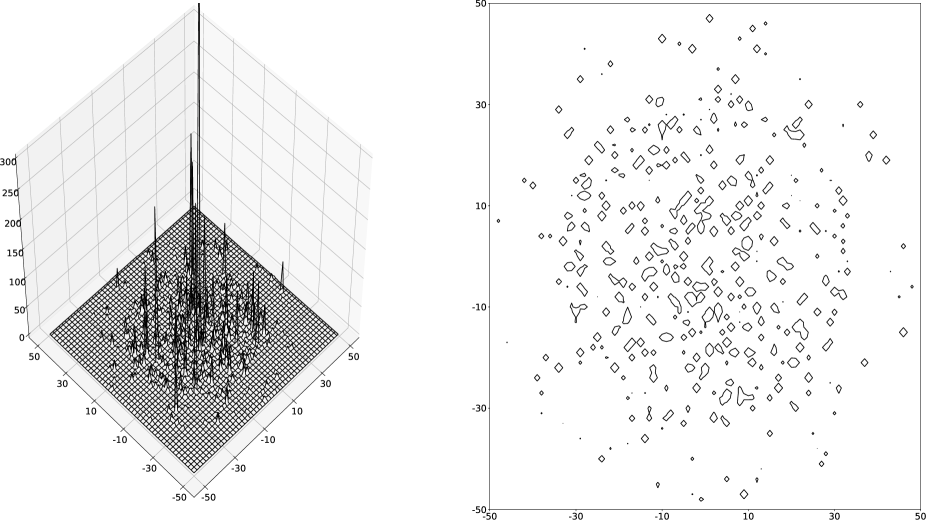
Figure 1: The simulated random field over $C=\{(x,y)\in\mathbb{Z}^{2}:x^{2}+y^{2}\leq 50^{2}\}$.

7 Conclusion

In the trajectories of a random field on a lattice, the propensity for oscillations, meaning the proportion of exceedances of high levels which are upcrossings, is inversely related to the degree of dependence and concordance between the random variables that generate it. We intended to quantify this propensity through coefficients that are easy to estimate and use in applications. We defined a crossinggram for max-stable random fields on lattices, which take values in [0,1] and are larger the more dependent and concordant the variables in the field are. These coefficients are related to the extremal coefficients usually found in the literature of extreme values. They also have a representation from the expected values of local maxima of the random field. This representation motivates the estimation method proposed and applied. The coefficients range from 0 to 1, where $0$ represents a very local rough random field and $1$ maximum local smoothness. The proposed estimator has Normal asymptotic distribution and can be used in practical applications. The proposed coefficients give good insight into the propensity for upcrossings by a max-stable random field from the theoretical point of view and in the example considered. They are easy to estimate and can be widely used.

References

- [1] Beirlant, J., Goegebeur, Y., Segers, J., Teugels, J. (2004) Statistics of Extremes: Theory and Applications. John Wiley & Sons, Hoboken.
- [2] Beirlant J., Escobar-Bach M., Goegebeur Y., Guillou A. (2016). Bias-corrected estimation of stable tail dependence function. Journal of Multivariate Analysis, 143, 453–466.
- [3] Davis, R., Mikosh, T. The extremogram: A correlogram for extreme events. Bernoulli 15(4), 2009, 977–1009.
- [4] Embrechts, P., Klüppelberg, C., Mikosch, T. Modelling Extremal Events for Insurance and Finance, Springer-Verlag, Berlin, 1997.
- [5] Escobar-Bach M., Goegebeur Y., Guillou A., (2018). Local estimation of the conditional stable tail dependence function. Scand. J. Stat., 45, 590–617, 2018.
- [6] Falk, M. and Tichy, D. (2012). Asymptotic conditional distribution of exceedance counts: fragility index with different margins. Annals of the Institute of Statistical Mathematics, Vol. 64, Issue 5, pp 1071–1085.
- [7] Ferreira, H., Ferreira, M. (2012a). On extremal dependence of block vectors. Kybernetika, 48(5), 988–1006.
- [8] Ferreira, H., Ferreira, M. (2012b). Fragility index of block tailed vectors. Journal of Statistical Planning and Inference, 142, 1837–1848.
- [9] Ferreira, H., Ferreira, M. (2018). Multidimensional extremal dependence coefficients. Statistics and Probability Letters, 133, 1–8.
- [10] Ferreira, H., Ferreira, M. Dissecting the multivariate extremal index and tail dependence. Accepted for publication in RevStat.
- [11] de Haan, L., Ferreira, A. (2006). Extreme Value Theory: An Introduction. Springer, Boston.
- [12] Joe, H. Multivariate Models and Dependence Concepts. Monographs on Statistics and Applied Probability 73, Chapman and Hall, London, 1997.
- [13] Kiriliouk, A., Segers, J., Tafakori, L. (2018). An estimator of the stable tail dependence function based on the empirical beta copula. Extremes 21, 581–600.
- [14] Ledford, A. W., Tawn, J. A. (1997). Modelling dependence within joint tail regions, J. Roy. Statist. Soc., B, 59, 475–499.
- [15] Li, H. Orthant tail dependence of multivariate extreme value distributions. Journal of Multivariate Analysis, 100, 243–256, 2009.
- [16] Naveau P., Guillou A., Cooley D., Diebolt J. (2009). Modeling Pairwise Dependence of Maxima in Space. Biometrika, 96, 1–17.
- [17] Ribatet, M., Dombry, C., Oesting, M. Spatial extremes and max-stable processes. In "Extreme value modeling and risk analysis: Methods and applications. Editors: Dey, D.K. and Yan, J., Taylor & Francis. 2016.
- [18] Shaked, M., Shanthikumar, G. (2007). Stochastic Orders. Springer-Verlag, New York.
- [19] Sibuya, M. Bivariate extreme statistics. Ann. Inst. Statist. Math., 11, 195–210, 1960.
- [20] Smith, R.L. Max-stable processes and spatial extremes, pre-print. University of North Carolina, USA, 1990.
- [21] Tiago de Oliveira, J. Structure theory of bivariate extremes, extensions. Est. Mat., Estat. e Econ., 7, 165–195, 1962/63.
- [22] Wadsworth, J. L., Tawn, J. A. (2012). Dependence modelling for spatial extremes. Biometrika, 99, 253–272.
- [23] Wadsworth, J. L., Tawn, J. A. (2013). A new representation for multivariate tail probabilities. Bernoulli, 19, 2689–2714.