Modeling cities

Abstract

Cities are systems with a large number of constituents and agents interacting with each other and can be considered as emblematic of complex systems. Modeling these systems is a real challenge and triggered the interest of many disciplines such as quantitative geography, spatial economics, geomatics and urbanism, and more recently physics. (Statistical) Physics plays a major role by bringing tools and concepts able to bridge theory and empirical results, and we will illustrate this on some fundamental aspects of cities: the growth of their surface area and their population, their spatial organization, and the spatial distribution of activities. We will present state-of-the-art results and models but also open problems for which we still have a partial understanding and where physics approaches could be particularly helpful. We will end this short review with a discussion about the possibility of constructing a science of cities.

I Introduction

Modeling cities and getting reliable quantitative predictions about their behavior have become major challenges for our modern world. Concentration of humans in a relatively small spatial area is essentially the result of economical considerations but spatial localization also leads to an increase of housing costs, traffic congestion, urban sprawl, pollution and other environmental problems. Organizing the city, building new infrastructures and new transportation means rely then a lot on our understanding of their effects on the collective behavior and their potential impact on the city, its functioning and its economical activity. This is particularly important at a time when we expect the number of megacities (with population larger than 10 millions) to be around 30 in 2050 UN: (see also Barthelemy (2016) for a more thorough discussion), and emergent countries see their cities exploding in size: it is estimated that by 2050 the world population will add 2.5 billion people to urban areas, with $90\%$ of this increase that will take place in Africa and Asia UN: .

From a theoretical point of view, cities comprise all the difficulties inherent to complex systems: a large variety of agents interacting with each other, a large variety of temporal and spatial scales, and a large number of processes that modify the spatial structure and organization of these systems. The always growing availability of urban data will hopefully help us to construct robust models and thereby to improve our knowledge of the main mechanisms at play during the evolution of urban systems. This fundamental level is necessary in order to construct robust computational models for describing more realistic or specific situations. Indeed, simulating the behavior of a urban system by ‘simply’ adding together all the possible processes and gathering as much information as possible, is neither a guarantee of its robustness, nor of the correctness of its predictions.

Economics and regional science were the first disciplines to tackle this problem of modeling cities. Most of the urban economics is built on the model proposed in the 60s by Alonso, Muth and Mills (see for example the textbook Fujita (1989) and references therein). This model relies on different assumptions. The first important one is that all individuals behave in the same way and maximize the same utility function subject to the same budget constraint. The second assumption is the monocentric city structure organized around a unique central business district (CBD). The information about transport infrastructure is here absent and space is considered as homogeneous and isotropic. All individuals are assumed to work at this CBD and the transportation cost depends on the distance from home to it (here we can see the impact of the first model proposed by Von Thunen Von Thunen and Hall (1966) with a unique market in an isolated state, where space is homogeneous and isotropic, and transportation cost depend only on the euclidean distance to the central market). Later, Fujita and Ogawa Fujita and Ogawa (1982) considered a general model where both individuals and firms are finding their optimal location in the city. In particular they introduced an agglomeration effect that describes the benefit for companies to be close to each other. These approaches constitute the basis of urban economics and we refer the interested reader to the books Fujita (1989); Fujita et al. (2001).

Agent-based models and large simulations also played an important role for understanding cities and were primarily developped by geographers in the 50-60s. The primary goal was to forecast the effects of planning policities and several formalisms were used Batty (2008); Pumain and Sanders (2013). The complexity of these simulations, the large number of parameters and processes however make it difficult to test thoroughly these models. In addition to these numerical simulations, it thus seems important to develop parsimonious models that help identifying the main mechanisms and to construct robust models. In this respect physics and more precisely statistical physics with its ability to connect microscopic behaviors to the emergence of collective and non-trivial behavior seems to be a particularly well-suited tool. In fact, statistical physics came into play later and connections with cities appeared first in the context of fractals and percolation. The fractal dimension of city boundaries was measured Batty and Longley (1994); Tannier and Pumain (2005) with a value between $1.2$ and $1.4$. The diffusion limited aggregation (DLA) model Witten and Sander (1983) was then naturally invoked to describe the growth of such a fractal structure. Later, statistical physicists Makse et al. (1995) proposed an alternative percolation model where the presence of correlations between new units is able to predict results in agreement with the dynamics of cities. This correlated percolation model Makse et al. (1998) is a very simplified model for cities, but nevertheless suggested the possible relevance of simple statistical physics approaches for systems as complex as cities. The importance of percolation in cities was reinforced in the study Rozenfeld et al. (2008) where the authors proposed a percolation-like algorithm to define cities without ambiguities, as the giant percolation cluster of the built-up area. Another important question where statistical physics contributed a lot is the social structure of cities. First discussed by Schelling Schelling (1971), agents are described by Ising like spins with tolerance level for other kinds and was later naturally rediscussed and improved by physicists Vinković and Kirman (2006); Grauwin et al. (2009); Gauvin et al. (2009); Dall’Asta et al. (2008); Jensen et al. (2018).

In this paper we won’t address all aspects of cities but we will focus on few of the most recent approaches that combine concepts and ingredients from economics and geography with tools and ideas from statistical physics. We will first discuss in sections II and III the – still relatively open – problem of the population and area growth of cities and their quantitative characterization. In particular, we will discuss a candidate model in direct connection with important problems in statistical physics for explaining the Zipf law that governs the statistics of urban populations. In section IV we will consider cities at a intra-urban level and discuss their spatial structure and the distribution of activities. Finally, in sections V and VI, we will discuss the issue about mixing together data for different cities and the possibility of constructing a ‘science of cities’ Batty (2013).

II Urban sprawl

A first and natural question about cities concerns their spatial extent and how it evolves in time. There are several definitions of cities but we will assume here a ‘functional’ definition where the city is not limited to its central core but includes peripheral areas that exchange enough commuters with it (for example MSA in the US or EU-OECD functional urban areas in Europe, see for example Bettencourt et al. (2013)). Another possibility is to consider the percolating cluster of built-up areas as in the ‘City clustering algorithm’ (CCA) discussed in Rozenfeld et al. (2008).

Cities and their built-up area are usually growing with time and the impact of urban sprawl on the environment has largely been debated and is highly politicized. There is however a relatively fair consensus about its negative impact on the environment (see for example Brueckner et al. (2000) and references therein) with the reduction of green areas, the increase of car traffic, the intensification of social segregation, and also the loss of physical activity and an increase of obesity Ewing et al. (2008). Despite the importance of the subject, the only studies available at this time are mostly purely statistical (such as multivariate analysis for example) and we don’t have a clear and simple quantitative model in agreement with data that could help us in identifying the critical factors of urban sprawl. We won’t discuss all studies about this important problem and we will start with a simple empirical discussion, followed by scaling arguments. We will then see how a statistical model can be constructed for this problem.

II.1 Empirical discussion

Visual inspection of the evolution of built-up areas of cities shows the existence of spreading phenomena, and ‘hotspots’ which suggests that nonlinear mechanisms are present (see Fig. 1).

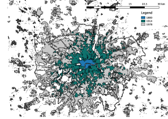
Figure 1: Evolution of the built-up area of London from 1800 to 1978 (the color-code indicates the age from blue to grey). We observe here the growth of a surface but the corresponding equation is not known yet. Data from Angel et al. (2005) and figure courtesy of E. Strano.

Despite these qualitative discussions, the quantitative description of this problem is completely open and we could expect that the physics of growing surface could help. In particular, finding an equation governing the spatio-temporal evolution of the local density would be a real breakthrough in our understanding of cities.

In order to go beyond visual and qualitative explorations, we plot the built-up area of various cities versus time and show the results in Fig. 2.

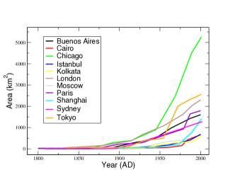
Figure 2: Evolution of the built area of various cities. These curves demonstrate an evolution faster than $t$ (typically as $t^{2}$ for most cities). Data from Angel et al. (2005).

We observe a large variety of behaviors that is difficult to understand without a theoretical guide, calling for the need of more empirical analysis and the construction of a theoretical framework. In particular, the range of variation does not allow here to characterize precisely the time behavior, even if we can see that in all case the area grows faster than $t$ (and is consistent in most cases with a $t^{2}$ behavior) implying at least a superdiffusive behavior.

Due to exogenous factors, time is probably not the most relevant variable and it seems quite natural to study the evolution of the cities surface area versus the population living in it, a long standing problem in the field (Makse et al. (1995)). Here also, we don’t have a clear picture yet. For cities in various countries, we can fit the data with a linear function of the form

$$A=aP$$ (1)

where $a$ is the inverse of the average density and represents the typical area per inhabitant. This corresponds to the intuitive expectation that cities evolve in such a way that their average population density $\rho=P/A$ remains constant. The quantity $a$ is the average surface occupied by each individual (the assumption of a constant density is equivalent to a constant average surface per capita). We can probably expect this behavior to hold for relatively small cities where there is an constant increase of the built-up area when the population is increasing. However, this regime is certainly limited as a city cannot extend indefinitely and we expect a later behavior characterized by a slower increase of the area. In some other cases, we can fit the data by a nonlinear function of the form

$$A=aP^{\tau}$$ (2)

where $\tau$ is an exponent usually slightly smaller than 1. In the linear case the density is contant $\rho=P/A=1/a$ and in the nonlinear case the density increases with population $\rho\sim P^{1-\tau}$: larger cities are also denser.

Empirically, we do observe that cities around the world display very different behaviors as shown in Fig. 3.

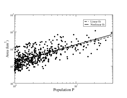
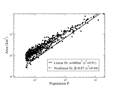
Figure 3: Area versus population for different regions in the world. (Left) Area of the 494 world cities with population larger than 1 million inhabitant. Both the linear and nonlinear fit are acceptable and very close to each other (data from various sources compiled by Wikipedia). (Right) US Urban areas with population over $50,000$ (data from the 2010 Census population). Here also both linear and nonlinear fits are acceptable and a more thorough statistical analysis is needed (such as in Leitão et al. (2016) for example).

When we mix together different countries of the world by taking urban areas with population larger than 1million (Fig. 3(left)), the nonlinear fit predicts an exponent slighly less than one ($\tau\approx 0.95$, $r^{2}=0.66$) and with this dataset it seems not possible to conclude between a constant density or a slightly increasing function of population (with exponent of order $0.05$). At a smaller scale, in the case of the US for example (Fig. 3(right)), the nonlinear behavior is also undistinguishable from the linear one. The linear fit predicts an average area of order $660m^{2}$ which is large, while the nonlinear fit gives an exponent $\beta\approx 0.87$. The linear fit predicts thus a constant density of order $1,500\mathrm{hab}/km^{2}$, which is correct for many cities, but we actually see deviations for large cities with density much larger for proper cities (and not for urban areas that mixes heterogeneous zones). For example for NYC, we have a density of order $10,000\mathrm{hab}/km^{2}$ or $6,600\mathrm{hab}/km^{2}$ for San Francisco. This behavior is however completely different for a country such as Japan for example (Fig. 4) where both linear and nonlinear fits are not good. The noise in this case cannot allow to conclude and the data suggests that the area is not a function of population only.

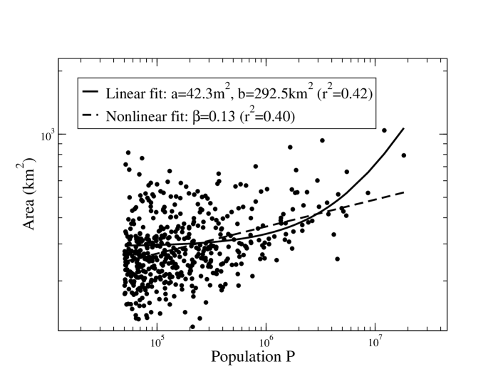
Figure 4: Area versus population for urban areas in Japan (data from the UN, Demographic Yearbook 2012).

After this little tour of empirical results, the absence of a clear stylized fact leaves us in the dark, and theoretical models, even very simplified ones, could shed some light on this problem. In order to illustrate how models could help us to understand the data, we will discuss here two different approaches to this problem: scaling and a statistical model based on dispersal ideas.

II.2 Scaling approach

Bettencourt Bettencourt (2013) proposed a phenomenological approach accounting for the value of the exponents governing the evolution of various quantities versus the population. In this approach the quantity of interest $Y$ can be any ‘urban socioeconomic output’ such as income, etc. Empirically we observe in general Pumain (2004); Bettencourt et al. (2007) a power law

$$Y\sim P^{\beta}$$ (3)

where $\beta$ is an exponent that can be different from 1. It was measured in Bettencourt et al. (2007) for various quantities and we can distinguish 3 groups according to its value. For social-related quantities (such as the number of patents, number of serious crimes, etc.), we observe $\beta>1$ possibly rooted in the fact that interactions in cities grow very fast with population, typically as $P^{2}$. In contrast, we also observe values $\beta<1$, which indicates an economy of scale (road surface, length of electric cables, etc.), and the last category with exponent $\beta=1$ comprises essentially quantities that do not depend on the size of the city (water consumption or other human-dependent quantities for example).

In order to estimate these exponents (and to obtain as a by-product the behavior of area with population), Bettencourt assumes that the economic output per capita $Y/P$ is proportional to the average number of interactions $Y/P\sim g\langle k\rangle$. The quantity $g$ is assumed to be constant and the average number of interactions is assumed to be $\langle k\rangle\sim\rho\sigma$ where $\sigma$ is the ‘cross-section’ of individuals and $\rho=P/A$ the average population density. This implies that

$$Y/P=G\frac{P}{A}$$ (4)

where $G$ is a constant. In addition, Bettencourt assumes that $Y/P$ is of the order of the cost of transport which is also proportional to the average distance $\ell$ travelled in the city. The average distance $\ell$ depends on the fractal dimension $H$ of the transportation network and Bettencourt writes $\ell\sim A^{H/d}$ (where usually $d=2$ is the dimension of the embedding space). We then have

$$Y/P\sim\frac{P}{A}\sim A^{H/d}$$ (5)

$$\Rightarrow A\sim P^{\frac{d}{H+d}}$$ (6)

Usually $d=2$, and in the simplest case of a linear transportation network $H=1$, we obtain $\beta=2/3$. This simple approach thus confirms a sublinear behavior with population but is at this point not able to explain the large fluctuations and the variety of behavior observed in real world cities.

II.3 A dispersal model

We are left with the question of constructing a simple model that is able to explain some of the features observed for the growth of the surface area of cities. A natural approach is to adapt dispersal models used in theoretical ecology. These models were developped to describe the proliferation of animal colonies Shigesada and Kawasaki (1997); Clark et al. (2001) and also as simplified models for cancerous tumor growth Iwata et al. (2000); Haustein and Schumacher (2012). The main feature of dispersal models is the concomitant existence of two growth mechanisms. The first process is the growth of the main (‘primary’) colony, which occurs typically via a reaction-diffusion process (for example as described by a FKK-like equation Fisher (1937); Shigesada and Kawasaki (2002)) and leads to a constant growth with a velocity $c$ that depends on the details of the system. In the case of urban systems, this process would correspond to new buildings constructed at the fringe of the city and which are in turn triggering the construction of new buildings. The second ingredient is random dispersal from the primary colony, which represents the emergence of secondary settlements. In the urban sprawl case, this second process corresponds to the creation of small towns in the periphery of large cities. In real-world systems, dispersion is not isotropic and is governed mainly by transportation systems (blood vessels in the case of metastatic tumors, winds and rivers in ecological examples), but in this first approach we will neglect these effects. We assume that these secondary colonies grow also at the velocity $c$ and eventually will coalesce with the primary colony. This image of a growing city, that eventually coalesces with neighboring small towns is consistent with our knowledge of urban growth (see for example the case of West London in Stanilov (2013)).

We will follow here the approach introduced by Kawasaki and Shigesada in Shigesada and Kawasaki (1997, 2002) in order to study this simplified model. We will consider that the primary colony grows at radial velocity $c$ and emits a secondary colony at a rate $\lambda$ and at a fixed distance $\ell$ from its border (long-range dispersal). Besides, we assume that each secondary colony also grows with the same radial speed $c$ and does not emit tertiary colonies. The dependence of the emission rate on the colony size is taken into account by the functional form

$$\lambda(r)=\lambda_{0}r^{\theta}~{},$$ (7)

$r$ being the radius of the primary colony and $\theta\geq 0$. When $\theta=0$ the growth rate is independent from the primary colony size, for $\theta=1$ it is proportional to its perimeter and for $\theta=2$ to its area. For cities, we can imagine that at least the perimeter or the surface are the relevant variables for triggering new towns in its surrounding and that $\theta\geq 1$ is therefore probably the most relevant for urban systems.

We consider two variants of this process Carra et al. (2017) - in a first version (model $M_{0}$) we assume that the primary colony remains circular after the coalescence with a secondary colony. In contrast, we can consider a modified version of the process (model $M_{1}$) where after the coalescence with a secondary colony, the shape of the primary colony does not remain circular. This important difference is illustrated in the Fig. 5.

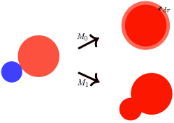
Figure 5: Example of coalescence in models $M_{0}$ and $M_{1}$. In $M_{0}$, the primary colony (in red) remains circular and the area of the secondary colony is evenly distributed on the rim; in $M_{1}$, the shapes are simply ‘concatenated’. Figure taken from Carra et al. (2017).

If we denote by $r(t)$ the radius of the primary colony at time $t$ and by $x(t)$ the radius of the colony absorbed at time $t$, we can show Carra et al. (2017) that the equations governing the evolution of these quantities are Shigesada and Kawasaki (2002); Carra et al. (2017)

$$\begin{cases}\frac{dr}{dt}&=c+\frac{\lambda_{0}{r\left(t-\frac{x(t)}{c}\right)}^{\theta}}{2\pi r(t)}\left(1-\frac{\dot{x}(t)}{c}\right)\pi x(t)^{2}~{},\\ \ell&=r(t)-r\left(t-\frac{x(t)}{c}\right)+x(t)~{}.\end{cases}$$ (8)

These nonlinear differential equations capture the physics of the coalescence and allows us to extract the large time behavior of the main quantities of interest in this problem. In particular, assuming scaling laws at large times, $r(t)\sim at^{\beta}$ and $x(t)\sim dt^{-\alpha}$, we obtain

$$\beta=\frac{3}{4-\theta}~{},\qquad\qquad\alpha=\beta-1~{}.$$ (9)

Note that for $\theta\rightarrow 4$, we have $\beta\rightarrow\infty$, the radius grows faster than a power law and explodes exponentially. For $\theta=1$, we obtain $\alpha=0,\beta=1$ which means that we have $x(t)=x^{*}$ independent of $t$ and a linear behavior of $r(t)$. In this case the effective radial velocity $c^{\prime}$ of the primary colony is given by

$$c^{\prime}=c+\frac{\lambda_{0}}{2}{x^{*}}^{2}$$ (10)

and the value of $x^{*}$ can be obtained by solving Eq. (8) that can be written as

$$\frac{\lambda_{0}}{2c}{x^{*}}^{3}+2{x^{*}}-\ell=0~{}.$$ (11)

This result, for the specific case of $\theta=1$, was first obtained by Shigesada and Kawasaki (Shigesada and Kawasaki, 1997). More generally, we can test our prediction for $\theta>1$ on numerical simulations, and in Fig. 6, we plot the values of the exponents $\beta$ obtained by power law fits and compare it with the theoretical prediction Eq. (9). We observe a good agreement with some deviations for higher values of $\theta$ which are probably due to finite size effect.

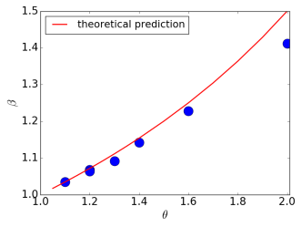
Figure 6: Plot of the exponent $\beta$ as a function of $\theta$, obtained from a power law fit on $r(t)$ versus $t$. The theoretical prediction Eq. (9) is shown in red. See Carra et al. (2017) for details.

Even if this model is very simple and is more ‘metaphorical’ than realistic Bouchaud (2019), it suggests that the simple mechanism of dispersal implies that the growth of the citie’s area (for $\theta\geq 1$) is scaling at least as $t^{2}$ in agreement with the empirical observations discussed above.

This simple Shigesada-Kawasaki coalescing model is based on the circular approximation and if we drop this assumption, analytical calculations seem out of reach. We can however investigate this problem numerically Carra et al. (2017) and assume that the area $A$ and the perimeter $L$ obey to a power law scaling of the form

$$A(t)\sim t^{\mu}\qquad L(t)\sim t^{\nu}~{}.$$ (12)

In the case of a constant emission rate $\lambda(r)=\lambda_{0}$, numerical results seem to show that $\mu\approx 2$ and $\nu\approx 1$. The dominant behavior are then $A(t)\sim\pi c^{2}t^{2}$ and $L(t)\sim 2\pi ct$. This shows that for $\theta=0$ and for large values of $t$, the circular approximation is valid: the city grows isotropically and absorbs neighboring towns. We can also consider the case where the emission rate $\lambda$ behaves as

$$\lambda(t)=\lambda_{0}L(t)~{},$$ (13)

where $L(t)$ is the total perimeter of the primary colony at time $t$. This case corresponds to $\theta=1$ in the model $M_{0}$. The simulations results for the area $A(t)$ and the perimeter $L(t)$ of the primary colony suggest that we still have $\mu\approx 2$ and $\nu\approx 1$ as in the $M_{0}$ model. We can go further and investigate the prefactors of $A(t)$ and $L(t)$. We recall that for the $M_{0}$ model with $\theta=1$, the radius of the primary colony increases with an effective radial velocity $c^{\prime}\neq c$. We can then study the quantities $A(t)/\pi c^{\prime 2}t^{2}-1$ and $L(t)/2\pi c^{\prime}t-1$; if the prefactor is the same of the $M_{0}$ model we should find (as we did for $\theta=0$) that these quantities tend to zero for large values of $t$. In fact we observe that these two quantities tend to a constant that depends on $\ell$. These results show that the circular approximation is not appropriate in the case described by Eq. 13 (see Fig. 7).

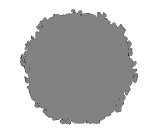
Figure 7: Example of shapes obtained for the model $M_{1}$. (Left) Constant emission rate and $\ell=10$. (Right) Emission rate proportional to the perimeter (Eq. 13), and $\ell=2$. Figures taken from Carra et al. (2017).

When the emission rate is proportional to the perimeter, the circular approximation thus breaks down and the roughness of the primary colony can not be discarded, thus modifying the scaling exponents. For cities, we expect that the rate of creation of new towns depends on the economical activity of the city and is at least proportional to its perimeter. These results show then that – independently from the anisotropy of transport networks – cities will in general not grow in an anisotropic way due to the coalescence with neighboring towns.

This model is of course very simplified and we are still far from a quantitative description of cities and their surface area, but we believe that this type of approach could serve as a basis for more elaborate ones and eventually to construct the equation governing the evolution of the area of cities.

III Modeling the population dynamics

The population of cities varies over several order of magnitudes: from small towns with hundreds of inhabitants to megacities with more than 10 million inhabitants. This large disparity of sizes has been noticed for some time already and Zipf uncovered in the 40s the ‘universal’ behavior of the form (see Zipf (1949))

$$P(R)\sim R^{-\nu}$$ (14)

where $P(R)$ is the population of the city at rank $R$ (cities are sorted in decreasing order according to their population). Interestingly enough, this result is robust and valid for different periods in time: even if there is a non-trivial microdynamics with the rank of cities changing all the time, Zipf’s law remains stable Batty (2006). The exponent $\nu$ is usually close to 1 for most countries which implies that the population distribution is close to $\rho(P)\sim 1/P^{2}$ (in general the population size distribution is a power law with exponent $\kappa=1+1/\nu$). More recent empirical evidences seem however to show that there are non-negligible fluctuations of this exponent (see Soo (2005) for an extensive study over 73 countries). The Zipf law has a number of interesting consequences: the ratio of the largest to second-largest city is given by $P_{1}/P_{2}=2^{1/\nu}$; for $\nu<1$ the largest city will have a population scaling as $P_{max}\sim N^{1/\nu}$; and the total population of a country scales as $W\sim N^{1/\nu}$ where $N$ is the number of cities.

Zipf’s law for cities triggered a huge number of studies in economics and also in physics and we discuss here some of the most important approaches together with an interesting connection with a classical model of statistical physics. First, Gibrat proposed in 1931 a simple rule stating that the growth rate of a firm is independent from its size Gibrat (1931), and applied to the growth of city populations, gives the following equation

$$P_{i}(t+1)=\eta_{i}(t)P_{i}(t)$$ (15)

where $P_{i}(t)$ is the population of city $i$ at time $t$ (usually the year). This equation basically describes the randomness of births and deaths by introducing an effective random growth rate $\eta_{i}(t)$ which is assumed to be independent from a city to another and without any time correlations. This simple equation with multiplicative noise naturally leads to a lognormal population distribution in contrast with empirical results, implying that the growth of urban areas is not consistent with Gibrat’s law. Several other approaches were then proposed in order to understand Zipf’s law Marsili and Zhang (1998); Gabaix (1999). In particular, Gabaix Gabaix (1999) proposed an alternative approach that is so far considered as the best explanation for Zipf’s law. It is based on the Gibrat model with the constraint that small cities cannot shrink to zero. In other words, the process considered by Gabaix is a random walk with a lower reflecting barrier which can, in some conditions, produce a power law distribution of populations. In addition to the reflecting barrier, a necessary condition is a drift towards the barrier and it is the combination of these two ingredients that can give rise to a power law Sornette and Cont (1997). The ‘regularization’ of the Gibrat model proposed by Gabaix relies on the assumption of a minimum size of cities and predicts the value $\nu=1$, but cities can actually disappear and this model is not completely satisfying. Ideally, we would like an approach based on reasonable mechanisms, linking micromotives with the large-scale behavior described by Zipf’s law. An interesting step towards such a description was proposed by Bouchaud and Mézard Bouchaud and Mézard (2000) (in the context of the wealth distribution) who discussed the diffusion equation with noise. This model has implications far beyond cities such as finance, directed polymers and the KPZ equation, etc. (see Bouchaud and Mézard (2000) and references therein). The diffusion equation with noise for the population $P_{i}(t)$ of city $i$ reads in the continuous time limit as

$$\frac{dP_{i}}{dt}=(\eta_{i}(t)-1)P_{i}(t)+\sum_{j}J_{ij}P_{j}(t)-J_{ji}P_{i}(t)$$ (16)

where the first term represents the ‘internal’ growth as given by Gibrat’s law and where the two last terms represent migrations between cities. We note that in contrast with some other models, the ingredients needed here are reasonable and correspond to a process that does occur in the real world. The random variables $\eta_{i}(t)$ are assumed to be identically independent Gaussian variables with the same mean and a variance given by $2\sigma^{2}$. The flow (per unit time) from city $i$ to $j$ is denoted by $J_{ji}$ and for a general form of these couplings we are unable to solve this equation. In the mean-field limit where all cities are exchanging individuals with each other ($J_{ij}=J/N$ where $N$ is the number of cities), Bouchaud and Mézard could show that the stationary distribution of the normalized population $w_{i}=P_{i}/\overline{P}$ (where $\overline{P}$ is the average population) is

$$\rho(w)\sim w^{-(1+\kappa)}\mathrm{e}^{-(\kappa-1)/w}$$ (17)

where the exponent is

$$\kappa=1+\frac{J}{\sigma^{2}}$$ (18)

When the migration term $J$ is nonzero, this regularization changes the lognormal distribution to a power law for large $w$ and the exponent is between 1 and 2 (for $J/\sigma^{2}<1$). The exponent $\kappa$ in this approach is not universal and depends on the details of the system providing a possible explanation for the diversity of values observed empirically Soo (2005). This diffusion model suggests an interesting connection between a central model in statistical physics and the old problem of the urban population distribution. It also shows that Zipf’s law finds its origin in the interplay between internal random growth and exchanges between different cities. An important consequence of this result is that increasing inter-urban mobility should actually increase $\kappa$ and therefore reduces the heterogeneity of the city size distribution. Other empirical tests are needed at this point, and from a theoretical point of view the mean-field assumption is not obvious. We expect that in general the couplings $J_{ij}$ are not constant and depend on the distance between cities, which could dramatically alter the results.

IV Spatial organization of cities

In this section, we will focus in the intra-urban scale. In particular, we will discuss approaches for understanding the spatial organization of a city. It is a problem of crucial importance as the location of residences and of the economic activity govern commuting flows and mobility patterns, a vital ingredient for assessing the efficiency of infrastructures and for planning. It is thus important to understand how households and companies choose a certain location and what are the main driving factors. We will first discuss here the main model used in urban economics and upon which many variants are constructed. We will then discuss another approach proposed by Krugman and which is a good example of a non-equilibrium approach to the city structure. Finally we will discuss a more recent model proposed in a statistical physics spirit.

IV.1 The Alonso-Muth-Mills model of urban economics

The Alonso-Muth-Mills (AMM) model is a pillar of urban economics and constitute the basis on which most economic models are constructed. In this respect we believe that it is important to know this model and we describe its main lines here. The first ingredient in this model is a utility function $U$ that describes the preferences of individuals (or households – they are usually considered to be the same in this simple approach) that are considered to be all equivalent. This function $U$ is usually assumed to depend on the land consumption $s$ (which corresponds to the surface area of apartments) and on the composite commodity $z$ (which corresponds to the money left when rent and transportation costs are substracted from the income)

$$U=U(z,s)$$ (19)

This utility has to satisfy the general constraints

$$\frac{\partial U}{\partial s}>0\;\;,\;\;\frac{\partial U}{\partial z}>0$$ (20)

which means that households in general prefer larger apartment and smaller costs. The budget constraint is given by

$$Y=z+T(x)+R(x)s$$ (21)

where $Y$ is the income of an household, $T(x)$ the transportation cost to work when living at location $x$ and $R(x)$ the renting cost per unit area at $x$. In this simplest version of the AMM model all households are renting their apartments and all landlords are living out of the city. The problem is then to optimize the utility subject to this budget constraint

$$\max_{z,s}U(z,s)\;\;\mathrm{subject\;\;to}\;\;Y=z+T(x)+R(x)s$$ (22)

This is a classical problem which can be solved with Lagrange multipliers, but we will here discuss a faster way to obtain general results. We introduce the constraint with $z=Y-sR-T$ and we maximize $U(Y-R(x)s-T(x),s)$ with respect to $s$

$$\frac{\partial U}{\partial s}=0=\partial_{1}U(-R(x))+\partial_{2}U$$ (23)

where $\partial_{i}U$ denotes the derivative of $U$ with respect to the $i^{th}$ variable. From this equation, we obtain the renting cost under the form

$$R(x)=\frac{\partial_{2}U}{\partial_{1}U}$$ (24)

An additional requirement is that the maximum utility $U^{*}$ should be independent from $x$. If it is not, then individuals could choose another better location and we wouldn’t be at equilibrium. We thus have to write

$$\frac{dU^{*}}{dx}=0=\partial_{1}U\left(-s\frac{dR}{dx}-R\frac{ds}{dx}-T^{\prime}(x)\right)+\partial_{2}U\frac{\partial s}{\partial x}$$ (25)

where the functions $s(x)$ and $R(x)$ are computed at equilibrium. Combining Eqs. (24) and (25) which are valid for all $x$, we then obtain the central result for the AMM model (see for example Brueckner (1987))

$$\frac{dR}{dx}=-\frac{T^{\prime}(x)}{s(x)}$$ (26)

This relation Eq. (26) allows us to discuss the location of individuals in the city. For example, for discussing the impact of income, we assume that transportation cost are linear in $x$ and then $T^{\prime}(x)=t$ and that we have two income categories, rich and poor characterized by their (fixed) land consumption $s_{R}$ and $s_{P}$, and transportation costs $t_{R}$ and $t_{P}$. The category of individuals that lives in a given area of the city is then the one that is willing to pay more for the rent at this location. The condition for the poor living in teh center can be shown to be

$$\frac{t_{P}}{s_{P}}>\frac{t_{R}}{s_{R}}$$ (27)

In the opposite case, rich individuals will live in the center as they are willing to pay more than the poor for this location (see Glaeser et al. (2008) for a detailed discussion about this point in the context of the AMM model).

We refer the interesting reader to the large litterature on the subject and in particular to the books Fujita (1989) and Fujita et al. (2001), and we will just make a few remarks about this approach. First, it assumes that cities are in equilibrium and their structure optimizes some objective function. Given the large variety of temporal (and spatial) scales, of processes and interactions, this assumption seems difficult to accept for cities. Even if we accept it, we are left with the difficult problem that some features of the city (such as the population profile for example) will actually depend on the precise form of the utility function. This poses the problem of the choice of the utility function and how to test it empirically. Also for this model, or for the more involved Fujita-Ogawa model (see Fujita and Ogawa (1982) and next sections), the theoretical predictions are usually not thoroughly tested against data. This is often true for classical studies of urban economics: theories and assumptions are not tested against data and serve as conceptual guides to understand some phenomena but usually with no clear guarantee of their validity.

IV.2 Krugman’s model: The Edge-City model

A non-equilibrium model for the spatial structure of cities and in particular how the economic activity clusters in specific regions was proposed by Krugman Krugman (1996). This approach is a good example of a minimal model that could probably be built upon and amenable to predictions that can be tested. The most important aspect here is the presence of interactions between firms. These interactions can lead to a polycentric organization of the city in which businesses are concentrated in spatially separated clusters. We follow the discussion proposed by Krugman (1996) and consider that the city is one-dimensional and the density of businesses is described by the function $\rho(x)$ whose integral is assumed to be constant. We assume that all locations are initially equivalent (which means in particular that there is relatively uniform transport infrastructure network) and the attractiveness of a location will depend on the spatial distribution of businesses. In order to describe this mathematically, Krugman introduces a quantity $\Pi(x)$ ‘a market potential’ which describes the level of attractivity of location $x$ and is given by

$$\Pi(x)=\int K(x-z)\rho(z)\mathrm{d}z$$ (28)

where the kernel is chosen as $K(x)=A(x)-B(x)$ with functions $A$ and $B$ that are both decreasing with the distance. These functions represent the positive and negative spillovers and how they vary with distance. Businesses will have an incentive to come to certain location depending on the level of attractiveness $\Pi$ and the simplest assumption is to compare $\Pi(x)$ to the average spatial level $\overline{\Pi}=\int\Pi(x)\rho(x)\mathrm{d}x$ and to write

$$\frac{d\rho(x)}{dt}=\gamma\left[\Pi(x)-\overline{\Pi}\right]$$ (29)

The density will then increase at locations where $\Pi(x)>\overline{\Pi}$ and decrease otherwise. This equation describes in a simple way the evolution of the business density with time and provide an explanation for the self-organized nature of cities. Note that since $\Pi(x)$ depends on $\rho$, the quantity $\overline{\Pi}=\int\Pi(x)\rho(x)\mathrm{d}x$ is nonlinear in $\rho$. Numerical simulations indicate that this nonlinear system indeed leads to various situations with multiple centers at different locations, depending on the initial conditions. Essentially, if positive spillovers are larger we will observe bigger clusters of businesses. We also see that this concentration has a reinforcement effect: regions with a large market potential will be more attractive and will therefore grow.

At a more quantitative level, we denote by $\lambda$ the size of spatial fluctuations and by $r_{1},r_{2}$ the range of positive and negative spillovers, respectively. For large frequencies, $\lambda\ll r_{1},r_{2}$ there is basically a compensation effect of positive and negative spillover and we do not expect the growth rate to be large. Also, for very low frequency fluctuations such as for example around a maximum of $\rho(x)$ which decays slowly around $x$, and for strong enough negative spillover, the growth rate at $x$ will be negative. Both low and high frequencies have thus negligible growth rate and it is natural to expect a frequency with a maximal growth rate, well-tuned to the spatial decay of positive and negative spillovers, leading to a specific spatial pattern in this city. In order to get a quick analytical insight, we can linearize the equation for $\rho(x)$ around the flat city $\rho(x)=\rho_{0}+\delta\rho(x)$ and find

$$\frac{d\delta\rho}{dt}\simeq\gamma\int K(x-z)\delta\rho(z)\mathrm{d}z+{\cal O}(\delta\rho^{2})$$ (30)

where we choose the normalization $\int\rho(x)=1$. Using the Fourier transform

$$\delta\rho(k)=\int\mathrm{e}^{ikx}\delta\rho(x)\mathrm{d}x$$ (31)

we obtain by integrating the linear differential equation

$$\delta\rho(k)\sim\mathrm{e}^{\gamma\hat{K}(k)}$$ (32)

where $\hat{K}(k)$ is the Fourier transform of the kernel $K(x)$. This expression shows that the Fourier mode $k^{*}$ for which $\hat{K}(k)$ is maximum will develop faster and will lead to the appearance of a spatial pattern characterized by $k^{*}$. We can obtain explicit expressions with the choice $K(x)=A\mathrm{e}^{-|x|/r_{1}}-B\mathrm{e}^{-|x|/r_{2}}$ which leads to

$$\frac{d\delta\rho(k,t)}{dt}=2\gamma\left[\frac{Ar_{1}}{1+(r_{1}k)^{2}}-\frac{Br_{2}}{1+(r_{2}k)^{2}}\right]\delta\rho(k,t)$$ (33)

We thus have for each mode a growth rate proportional to

$$\Lambda(k)=\frac{Ar_{1}}{1+(r_{1}k)^{2}}-\frac{Br_{2}}{1+(r_{2}k)^{2}}$$ (34)

which satisfies $\Lambda(0)=A-B$ which is negative for large enough $B$ and $\Lambda(k)\to 0$ for $k$ large. We thus expect in general a maximum $\Lambda^{*}$ for a value $k^{*}$ that can be easily computed. This value $k^{*}$ depends here on $r_{1},r_{2},A$ and $B$ and is thus finite and independent from the city size. For a one dimensional city of size $L$, the number of business clsuters is then given by

$$H\sim Lk^{*}$$ (35)

This simple model thus predicts a linear increase of the number of activity centers (or ‘hostspots’) with city size, but doesn’t explain in particular how this quantity scales with population. Indeed, new datasources such as cell phone networks, employment data, smart card transactions and taxi GPS trajectories provide a lot of information about cities and their structure. In particular, it has been shown Louf and Barthelemy (2013); Louail et al. (2014) that the number $H$ of activity centers (or ‘hotspots’) is scaling with population as

$$H\sim P^{\sigma}$$ (36)

where the exponent $\sigma$ is found to be around $0.5-0.6$. The number of these hotspots thus scales sublinearly with the population size, a result that will serve as a guide for constructing a theoretical model. We thus see that Krugman’s model is not able to explain this behavior. Although it is interesting to see how simple nonlinear effects give rise to a nontrivial spatial pattern, this model doesn’t produce at this stage predictions that are directly testable on empirical data.

IV.3 A variant of Fujita-Ogawa

The Krugman model discussed above is unable to explain the empirical behavior Eq. (36). We will show here how a simplified variant of the Fujita-Ogawa model Fujita and Ogawa (1982) can actually help us to understand this empirical result. We start from the standard economical assumption that an invidivual will choose a residence located at $x$ and to work at location $y$ such that the quantity

$$Z(x,y)=W(y)-C_{R}(x)-T(x,y)$$ (37)

is maximum. The quantity $W(y)$ is the typical wage earned at location $y$, $C_{R}(x)$ is the rent cost at $x$, and $T(x,y)$ is the transportation cost to go from $x$ to $y$ and is usually taken to be proportional to the time $\tau(x,y)$ spent to cover this distance. In their original paper, Fujita and Ogawa Fujita and Ogawa (1982) couldn’t find the general solution, but tested the stability of some specific urban forms. For example, by neglecting congestion and writing $\tau(x,y)=d(x,y)/\overline{v}$ (where $d(x,y)$ is the euclidean distance between $x$ and $y$ and $\overline{v}$ is the free flow average velocity), they could show that if the transportation cost for the typical interaction distance between companies becomes too large, the monocentric organization with a central business district surrounded by residential areas is unstable. However, this formalism does not allow to predict the resulting urban structure, and we have to simplify it in order to reach testable predictions. First, we assume that each agent has a residence located at random. Second, a quantity as complex as the wage results from a large number of interactions and factors, and it is tempting – in the spirit of random Hamiltonians for heavy ions Dyson (1962) – to replace this complex quantity by a random number $\phi(y)$: $W(y)=s\phi(y)$ where $s$ sets the salary scale (and with a certain distribution of $\phi$ which is irrelevant at this point). Last but not least, we assume that most of the displacements are made by car and we include congestion effect which implies that the time $\tau(x,y)$ depends on the traffic $Q(x,y)$ as described by the simple Bureau of Public Roads function (see for example Branston (1976))

$$\tau(x,y)=\frac{d(x,y)}{\overline{v}}\left[1+\left(\frac{Q(x,y)}{C}\right)^{\mu}\right]$$ (38)

where $C$ is the road system capacity, and $\mu$ an exponent, usually between 2 and 5. These ingredients put together allow for a simple mean-field analysis showing that the monocentric organization is unstable for a value of the population larger than a threshold $P^{*}$ (which depends on the details of the city) and that the number $H$ of distinct activity centers is given by

$$H\sim\left(\frac{P}{P^{*}}\right)^{\frac{\mu}{\mu+1}}$$ (39)

(see Fig. 8). This simplified model thus predicts a sublinear behavior for the number of activity centers with an exponent given by $\sigma=\mu/(\mu+1)$ (for $\mu\approx 2$, we then recover the empirical value $\sigma\approx 0.6$, and for $\mu=0$ we have $H\sim{\cal O}(1)$ in the absence of congestion). We observe that whatever the value of $\mu$, the behavior is sublinear, and congestion appears as a critical factor that shapes the structure of the city and favors the appearance of new activity centers.

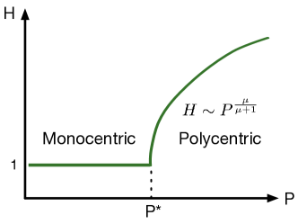
Figure 8: Number of activity centers versus the population for the model discussed in the text: we observe a monocentric-polycentric transition for a value $P^{*}$ that depends on the city.

Finally, we note that knowing both the residence and workplace locations allows to discuss multiple aspects of the commuting to work Louf and Barthelemy (2014). In particular, we can estimate the total commuting time and the quantity of CO₂ emitted by cars (see also Verbavatz and Barthelemy (2019)).

V Averaging over many cities ?

Various studies of cities such as scaling Bettencourt et al. (2007) use data from different cities at different times and plot some quantity versus population. For many quantities (denoted $Y$ here), we observe a power law of the form $Y\sim P^{\beta}$ where $P$ is the population of the city Bettencourt et al. (2007). As we already discussed above, we can distinguish different behavior according to the value of $\beta$, in particular if it is larger than one or not. Once we have measured this scaling form, we could in principle use it for predicting the behavior of an individual city when its population changes. In order to illustrate the possible problems of such an approach we consider the particular case of delays due to traffic congestion and analyze a dataset for 101 US cities in the time range 1982-2014 Depersin and Barthelemy (2018). This is a particularly interesting dataset as it is both transversal – it contains many cities – and longitudinal – for each city we have the temporal evolution of the delay.

The scaling form obtained by agglomerating all the available data for different cities and for different years displays a nonlinear behavior, seemingly in agreement with general empirical results about scaling Bettencourt et al. (2007).

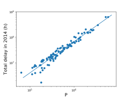
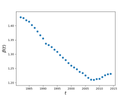
Figure 9: (Top) Plot of the annual delay $\delta\tau$ versus the number of drivers $P$ for all cities in 2014. The straight line is a power law fit in this loglog representation and gives an exponent value $\beta\approx 1.23$ (and $R^{2}=0.93$). (Bottom) Scaling exponent $\beta(t)$ for the delay computed for each year separately, from 1982 to 2014. All these values are consistent with a superlinear behavior found in Chang et al. (2017). Figure taken from Depersin and Barthelemy (2018).

More precisely, we can first compute the scaling exponent by mixing together all cities but for a given year. We can also compute this exponent for each year and we observe an exponent whose value varies in the range $[1.2,1.4]$ for years from 1982 to 2014 (see Fig. 9). Finally, we can consider all cities and for all years and we then obain a delay in traffic jams scaling as

$$\delta\tau\sim P^{\beta}$$ (40)

with $\beta\approx 1.36$ consistent with a superlinear behavior.

However, if we don’t average over the different cities, we observe the behaviors shown by different colors in the Fig. 10.

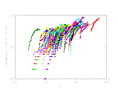
Figure 10: Annual delay per capita $\delta\tau/P$ versus $P$ for all the 101 cities and for all years (1982 – 2014). The points are colored according to the city they describe (one color per city). As we discuss in the text there is no obvious relation between the global power-law scaling and the individual behavior of cities. Figure taken from Depersin and Barthelemy (2018).

The different cities display then a variety of behaviors ranging from pure power laws with exponents larger than one, or two power laws, etc. (see Depersin and Barthelemy (2018) for details). The scaling obtained by averaging over all cities appears then completely unrelated to the dynamics of individual cities when their population grow. There seems to be no simple scaling at the individual city level but a variety of behaviors. In the language of statistical physics, the delay is not a state function determined by the population only, and displays some sort of aging effect where it depends not on the population only but also on time, and probably on the whole history of the city. This idea of path-dependency is natural for many complex systems, and in particular in statistical physics (such as spin-glasses Bouchaud et al. (1998) for example). The delay is not a simple function of population as it is usually assumed for the scaling approach for cities, and if we reflect upon this idea, it doesn’t make sense in general to compare two cities having the same population but at very different dates: both central Paris and Phoenix (AZ) had a population of about 1 million inhabitants, the former in 1840 and the latter in 1990. It is very likely that the dynamics – for many quantities – from 1840 in Paris will be very different from the one starting in 1990 in Phoenix, implying that the usual scaling form does not apply in general. This discussion on congestion induced delays highlights the risk of agglomerating data for different cities and to consider that cities are scaled-up versions of each other: there are strong constraints for being allowed to do that such as path-independence, which is apparently not satisfied in the case of congestion and which should be checked in each case. Beyond scaling, these results also pose the challenging problem of using transversal data (ie. for different cities) in order to get some information about the temporal series for individual cities. This is a fundamental problem that needs to be clarified when looking for generic properties of cities.

VI Perspectives

Many aspects and studies about cities were not addressed in this paper: the evolution of infrastructure networks Strano et al. (2012); Levinson and Yerra (2006), the coupling between networks Kivelä et al. (2014), multimodality Gallotti and Barthelemy (2014); Strano et al. (2015), heat islands and urban forms Sobstyl et al. (2018), etc. An important point here was to show through various examples how a combination of empirical results, economical ingredients, and statistical physics tools can lead to parsimonious models with predictions in agreement with observations. In particular, describing individual actions by stochastic processes and replacing complex quantities resulting from the interactions of several agents by random variables, seem to be a good way to construct models for understanding the evolution of cities and in agreement with empirical observations.

We however still have to think about the best approach for understanding complex systems such as cities. Is it possible to construct a generic model of cities that can predict general trends and behaviors ? In this perspective, a particular city would then just be described by this generic model subject to local spatial and historical constraints. In other words, this assumption means that all cities belong to the same species but each individual city evolved on a different substrate. As we saw in this short review, this possibility and the existence of generic behaviors is not empirically clear. We do observe generic properties such as the Zipf law and mixing together different cities doesn’t seem to pose a problem in this case, in contrast with the exemple of congestion induced delays. There is however the risk that this debate becomes quickly outdated as machine learning displays impressive results in practical applications. At least, we could always hope that parsimonious models have the advantage to provide a simple language for making sense of the vast amount of data and to identify critical factors for the evolution of these systems.

References

- [1] United nations, world urbanization prospects, 2018. URL https://esa.un.org/unpd/wup/.
- Barthelemy [2016] Marc Barthelemy. The structure and dynamics of cities. Cambridge University Press, 2016.
- Fujita [1989] Masahisa Fujita. Urban economic theory: land use and city size. Cambridge University Press, 1989.
- Von Thunen and Hall [1966] Johann Heinrich Von Thunen and Peter Geoffrey Hall. Isolated state. Pergamon, 1966.
- Fujita and Ogawa [1982] Masahisa Fujita and Hideaki Ogawa. Multiple equilibria and structural transition of non-monocentric urban configurations. Regional science and urban economics, 12(2):161–196, 1982.
- Fujita et al. [2001] Masahisa Fujita, Paul R Krugman, and Anthony J Venables. The spatial economy: Cities, regions, and international trade. MIT press, 2001.
- Batty [2008] Michael Batty. Fifty years of urban modeling: Macro-statics to micro-dynamics. In The dynamics of complex urban systems, pages 1–20. Springer, 2008.
- Pumain and Sanders [2013] Denise Pumain and Lena Sanders. Theoretical principles in interurban simulation models: a comparison. Environment and Planning A, 45(9):2243–2260, 2013.
- Batty and Longley [1994] Michael Batty and Paul A Longley. Fractal cities: a geometry of form and function. Academic Press, 1994.
- Tannier and Pumain [2005] Cécile Tannier and Denise Pumain. Fractals in urban geography: a theoretical outline and an empirical example. Cybergeo: European Journal of Geography, 2005.
- Witten and Sander [1983] Thomas A Witten and Leonard M Sander. Diffusion-limited aggregation. Physical Review B, 27(9):5686, 1983.
- Makse et al. [1995] Hernén A Makse, Shlomo Havlin, and HE Stanley. Modelling urban growth. Nature, 377:19, 1995.
- Makse et al. [1998] Hernán A Makse, José S Andrade, Michael Batty, Shlomo Havlin, H Eugene Stanley, et al. Modeling urban growth patterns with correlated percolation. Physical Review E, 58(6):7054, 1998.
- Rozenfeld et al. [2008] Hernán D Rozenfeld, Diego Rybski, José S Andrade, Michael Batty, H Eugene Stanley, and Hernán A Makse. Laws of population growth. Proceedings of the National Academy of Sciences, 105(48):18702–18707, 2008.
- Schelling [1971] Thomas C Schelling. Dynamic models of segregation†. Journal of mathematical sociology, 1(2):143–186, 1971.
- Vinković and Kirman [2006] Dejan Vinković and Alan Kirman. A physical analogue of the schelling model. Proceedings of the National Academy of Sciences, 103(51):19261–19265, 2006.
- Grauwin et al. [2009] Sébastian Grauwin, Eric Bertin, Rémi Lemoy, and Pablo Jensen. Competition between collective and individual dynamics. Proceedings of the National Academy of Sciences, 106(49):20622–20626, 2009.
- Gauvin et al. [2009] Laetitia Gauvin, Jean Vannimenus, and J-P Nadal. Phase diagram of a schelling segregation model. The European Physical Journal B, 70(2):293–304, 2009.
- Dall’Asta et al. [2008] Luca Dall’Asta, Claudio Castellano, and Matteo Marsili. Statistical physics of the schelling model of segregation. Journal of Statistical Mechanics: Theory and Experiment, 2008(07):L07002, 2008.
- Jensen et al. [2018] Pablo Jensen, Thomas Matreux, Jordan Cambe, Hernan Larralde, and Eric Bertin. Giant catalytic effect of altruists in schelling’s segregation model. Physical Review Letters, 120(20):208301, 2018.
- Batty [2013] Michael Batty. The New Science of Cities. MIT Press, 2013.
- Bettencourt et al. [2013] Luis Bettencourt, Jose Lobo, and Hyejin Youn. The hypothesis of urban scaling: formalization, implications and challenges. arXiv preprint arXiv:1301.5919, 2013.
- Brueckner et al. [2000] Jan K Brueckner et al. Urban sprawl: diagnosis and remedies. International regional science review, 23(2):160–171, 2000.
- Ewing et al. [2008] Reid Ewing, Tom Schmid, Richard Killingsworth, Amy Zlot, and Stephen Raudenbush. Relationship between urban sprawl and physical activity, obesity, and morbidity. In Urban Ecology, pages 567–582. Springer, 2008.
- Angel et al. [2005] Shlomo Angel, Stephen Sheppard, Daniel L Civco, Robert Buckley, Anna Chabaeva, Lucy Gitlin, Alison Kraley, Jason Parent, and Micah Perlin. The dynamics of global urban expansion. Citeseer, 2005.
- Leitão et al. [2016] Jorge C Leitão, José María Miotto, Martin Gerlach, and Eduardo G Altmann. Is this scaling nonlinear? Royal Society open science, 3(7):150649, 2016.
- Bettencourt [2013] Luís MA Bettencourt. The origins of scaling in cities. science, 340(6139):1438–1441, 2013.
- Pumain [2004] Denise Pumain. Scaling laws and urban systems. Santa Fe Institute, Working Paper n 04-02, 2:26, 2004.
- Bettencourt et al. [2007] Luís MA Bettencourt, José Lobo, Dirk Helbing, Christian Kühnert, and Geoffrey B West. Growth, innovation, scaling, and the pace of life in cities. Proceedings of the National Academy of Sciences, 104(17):7301–7306, 2007.
- Shigesada and Kawasaki [1997] N. Shigesada and K. Kawasaki. Invasion by stratified diffusion, chapter 5, page 79–103. Oxford University Press, USA, 1997.
- Clark et al. [2001] J.S. Clark, M. Lewis, and Horvath L. Invasion by extremes: Population spread with variation in dispersal and reproduction. The American Naturalist, 157(5):537–554, 2001.
- Iwata et al. [2000] K. Iwata, K. Kawasaki, and N. Shigesada. A dynamical model for the growth and size distribution of multiple metastatic tumors. J. Theor. Biol., 203(2):177–186, 2000.
- Haustein and Schumacher [2012] V Haustein and U Schumacher. A dynamical model for tumour growth and metastasis formation. J. Clin. Bioinforma., 2(1), 2012.
- Fisher [1937] Ronald Aylmer Fisher. The wave of advance of advantageous genes. Annals of Human Genetics, 7(4):355–369, 1937.
- Shigesada and Kawasaki [2002] N. Shigesada and K. Kawasaki. Invasion and the range expansion of species: effects of long-distance dispersal, chapter 17, page 350–373. Blackwell Science, 2002.
- Stanilov [2013] Kiril Stanilov. Planning the growth of a metropolis: factors influencing development patterns in west london, 1875–2005. Journal of Planning History, 12(1):28–48, 2013.
- Carra et al. [2017] Giulia Carra, Kirone Mallick, and Marc Barthelemy. Coalescing colony model: Mean-field, scaling, and geometry. Physical Review E, 96(6):062316, 2017.
- Bouchaud [2019] Jean-Philippe Bouchaud. Econophysics: Still fringe after 30 years? arXiv preprint arXiv:1901.03691, 2019.
- Zipf [1949] George Kingsley Zipf. Human behavior and the principle of least effort. addison-wesley press, 1949.
- Batty [2006] Michael Batty. Rank clocks. Nature, 444(7119):592–596, 2006.
- Soo [2005] Kwok Tong Soo. Zipf’s law for cities: a cross-country investigation. Regional science and urban Economics, 35(3):239–263, 2005.
- Gibrat [1931] Robert Gibrat. Les inégalités économiques. Recueil Sirey, 1931.
- Marsili and Zhang [1998] Matteo Marsili and Yi-Cheng Zhang. Interacting individuals leading to zipf’s law. Physical Review Letters, 80(12):2741, 1998.
- Gabaix [1999] Xavier Gabaix. Zipf’s law for cities: an explanation. Quarterly journal of Economics, pages 739–767, 1999.
- Sornette and Cont [1997] Didier Sornette and Rama Cont. Convergent multiplicative processes repelled from zero: power laws and truncated power laws. Journal de Physique I, 7(3):431–444, 1997.
- Bouchaud and Mézard [2000] Jean-Philippe Bouchaud and Marc Mézard. Wealth condensation in a simple model of economy. Physica A: Statistical Mechanics and its Applications, 282(3):536–545, 2000.
- Brueckner [1987] Jan K Brueckner. The structure of urban equilibria: A unified treatment of the muth-mills model. Handbook of regional and urban economics, 2:821–845, 1987.
- Glaeser et al. [2008] Edward L Glaeser, Matthew E Kahn, and Jordan Rappaport. Why do the poor live in cities? the role of public transportation. Journal of urban Economics, 63(1):1–24, 2008.
- Krugman [1996] Paul R Krugman. The self-organizing economy. Blackwell Oxford, 1996.
- Louf and Barthelemy [2013] Rémi Louf and Marc Barthelemy. Modeling the polycentric transition of cities. Physical Review Letters, 111(19):198702, 2013.
- Louail et al. [2014] Thomas Louail, Maxime Lenormand, Oliva G Cantu Ros, Miguel Picornell, Ricardo Herranz, Enrique Frias-Martinez, José J Ramasco, and Marc Barthelemy. From mobile phone data to the spatial structure of cities. Scientific reports, 4, 2014.
- Dyson [1962] Freeman J Dyson. Statistical theory of the energy levels of complex systems. i. Journal of Mathematical Physics, 3(1):140–156, 1962.
- Branston [1976] David Branston. Link capacity functions: A review. Transportation Research, 10(4):223–236, 1976.
- Louf and Barthelemy [2014] Rémi Louf and Marc Barthelemy. How congestion shapes cities: from mobility patterns to scaling. Scientific Reports, 4, 2014.
- Verbavatz and Barthelemy [2019] Vincent Verbavatz and Marc Barthelemy. Critical factors for mitigating car traffic in cities. arXiv preprint arXiv:1901.01386, 2019.
- Depersin and Barthelemy [2018] Jules Depersin and Marc Barthelemy. From global scaling to the dynamics of individual cities. Proceedings of the National Academy of Sciences, 115(10):2317–2322, 2018.
- Chang et al. [2017] Yu Sang Chang, Yong Joo Lee, and Sung Sup Brian Choi. Is there more traffic congestion in larger cities?-scaling analysis of the 101 largest us urban centers. Transport Policy, 59:54–63, 2017.
- Bouchaud et al. [1998] Jean-Philippe Bouchaud, Leticia F Cugliandolo, Jorge Kurchan, and Marc Mezard. Out of equilibrium dynamics in spin-glasses and other glassy systems. Spin glasses and random fields, pages 161–223, 1998.
- Strano et al. [2012] Emanuele Strano, Vincenzo Nicosia, Vito Latora, Sergio Porta, and Marc Barthelemy. Elementary processes governing the evolution of road networks. Scientific reports, 2, 2012.
- Levinson and Yerra [2006] David Levinson and Bhanu Yerra. Self-organization of surface transportation networks. Transportation Science, 40(2):179–188, 2006.
- Kivelä et al. [2014] Mikko Kivelä, Alex Arenas, Marc Barthelemy, James P Gleeson, Yamir Moreno, and Mason A Porter. Multilayer networks. Journal of Complex Networks, 2(3):203–271, 2014.
- Gallotti and Barthelemy [2014] Riccardo Gallotti and Marc Barthelemy. Anatomy and efficiency of urban multimodal mobility. Scientific reports, 4, 2014.
- Strano et al. [2015] Emanuele Strano, Saray Shai, Simon Dobson, and Marc Barthelemy. Multiplex networks in metropolitan areas: generic features and local effects. Journal of The Royal Society Interface, 12(111):20150651, 2015.
- Sobstyl et al. [2018] JM Sobstyl, T Emig, MJ Abdolhosseini Qomi, F-J Ulm, and RJ-M Pellenq. Role of city texture in urban heat islands at nighttime. Physical Review Letters, 120(10):108701, 2018.