Supplemental Material: Precision Test of the Limits to Universality in Few-Body Physics

I Summary of the Synergism between Theory and Experiment

Besides providing the details of some of the experimental and theoretical implementation of our studies, this supplementary material also provides the details on how theory and experiment worked together in order to produce highly accurate results. Our studies for the binding energies of Feshbach molecules (described in Section II) required a theoretical model consisting of a fully coupled channel approach Chin et al. (2010) where realistic singlet and triplet Born-Oppenheimer potentials are used, supporting many dozens of $s$-wave molecular states, and still many more molecular states with non-vanishing orbital angular momenta. Such potentials were derived in Ref. Falke et al. (2008) based on previous spectroscopic data allowing for the precise characterization of the singlet and triplet scattering lengths. Nevertheless, our current experimental data surpass that precision. Therefore, we further fine tune the potentials in order to fit our data and produce more refined values for the scattering lengths, the width and the position of the corresponding Feshbach resonance. The refinement procedure is described in Section II.

Although our two-body model with realistic singlet and triplet potentials Falke et al. (2008) can describe our data for the binding energies quite accurately, this model is not suitable for performing three-body calculations due to the high number of molecular states the potentials can support, leading to a prohibitively large number of three-body channels to be described numerically. In our three-body approach Wang et al. (2011, 2012a, 2012b); Mestrom et al. (2017); Suno et al. (2002) we determined the solutions of a system of two-dimensional partial differential equations which become highly oscillatory depending on the number of molecular states the potential can support, making it difficult to reach the necessary accuracy for our problem. In order to obtain a more numerically manageable model we replace the realistic singlet and triplet potentials by model potentials containing a much smaller number of bound states but still preserving the correct values for the singlet and triplet scattering lengths. Our three-body calculations use these reduced two-body models for different potentials containing a variable number of bound states in order to test their universality. This procedure is described in more detail in Section III.

II Dimer Binding Energy Spectroscopy

II.1 Binding Energy Data

A compilation of the $E_{b}$ spectroscopy data is presented in Table 1. We take atomic spectra before and after each dimer dissociation measurement. The weighted mean $\bar{f}_{\mathrm{A}}$ of the two atomic lineshape centers ($f_{\mathrm{A,1}}$ and $f_{\mathrm{A,2}}$) defines the free-free transition frequency and, via the Breit-Rabi formula, the magnetic field $B$. To extract the bound-free dissociation threshold frequency, we subtract $\bar{f}_{\mathrm{A}}$ from the measured dimer dissociation spectrum and fit the spectrum to a function (see Fig. S.1) that is a convolution of the Franck-Condon factor Chin and Julienne (2005) and the Fourier-spectrum of the Gaussian-shaped RF dissociation pulse, whose duration, spanning $600\,\mu$s at high $E_{b}$ to $12\,$ms at low $E_{b}$, is chosen to be shorter than the dimer lifetime. The total uncertainty on the dissociation threshold frequency is taken as the fit error added in quadrature with uncertainty on $\bar{f}_{\mathrm{A}}$. Finally, we extract the free-space dimer binding energy $E_{b}$ by subtracting the total confinement-related frequency shift from the dissociation threshold frequency. We calculate the confinement shift for the final (free) and initial (bound) states and take their difference as the total confinement shift Idziaszek and Calarco (2006). Due to relatively small trap frequencies of $\omega_{r}/2\pi=28.64(66)\thinspace$Hz and $\omega_{z}/2\pi=117.3(1.0)\thinspace$Hz and the final state being nearly non-interacting, the total confinement shift is equal, within uncertainty on our trapping frequencies, to the zero-point energy $87.3(1.4)\thinspace$Hz for all dissociation spectra.

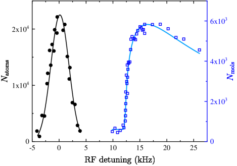
Figure S.1: RF spectra of free-free transition (circles) and bound-free transition (squares) at $B=33.9575(3)\thinspace$G, where the RF frequency is detuned from $446.834413\thinspace$MHz. Values $N_{\mathrm{atoms}}$ and $N_{\mathrm{mols}}$ are proportional to the number of atoms and molecules detected during spectroscopy. The frequency difference between the atomic spectrum (black line) center and the onset of the dimer dissociation spectrum (blue line) corresponds to the dissociation threshold frequency in the confining trap.

Table 1: Precise binding energy spectroscopy data. The $B$–field is determined from the weighted mean $\bar{f}_{\mathrm{A}}$ of two atomic lineshape centers $f_{\mathrm{A,1}}$ and $f_{\mathrm{A,2}}$, taken before and after each molecular dissociation spectrum. The frequency $f_{\mathrm{D}}$ corresponds to the dissociation threshold frequency in the confining trap, while $E_{b}$ corresponds to the free-space dimer binding energy.

free-free transition	free-free transition	free-free transition	magnetic field	confined dissociation	free-space
center $f_{\mathrm{A,1}}$	center $f_{\mathrm{A,2}}$	mean $\bar{f}_{\mathrm{A}}$	$B$	threshold $f_{\mathrm{D}}-\bar{f}_{\mathrm{A}}$	$E_{b}/h$
(MHz)	(MHz)	(MHz)	(G)	(kHz)	(kHz)
446.870873(67)	446.870945(63)	446.870911(52)	33.7420(3)	2.190(56)	2.103(56)
446.861460(78)	446.861312(76)	446.861384(76)	33.7978(4)	3.989(78)	3.901(78)
446.852714(79)	446.852546(82)	446.852634(82)	33.8494(5)	6.095(85)	6.008(85)
446.834376(61)	446.834445(57)	446.834413(48)	33.9575(3)	12.274(57)	12.187(57)
446.826070(69)	446.825957(59)	446.826004(60)	34.0078(4)	15.708(67)	15.621(67)
446.816781(61)	446.817086(55)	446.816950(116)	34.0622(7)	20.139(122)	20.052(122)
446.800019(79)	446.800145(76)	446.800085(71)	34.1644(4)	29.919(83)	29.832(83)
446.783321(76)	446.783547(73)	446.783439(96)	34.2663(6)	41.847(103)	41.760(103)
446.748851(78)	446.748911(73)	446.748883(57)	34.4812(4)	74.382(93)	74.295(93)
446.731051(77)	446.731033(101)	446.731045(61)	34.5940(4)	95.395(137)	95.307(137)
446.667723(82)	446.667598(77)	446.667657(71)	35.0060(5)	200.293(406)	200.205(406)
446.621332(86)	446.621191(74)	446.621252(75)	35.3198(5)	308.716(436)	308.628(436)
446.559027(89)	446.558891(79)	446.558951(76)	35.7593(6)	508.003(582)	507.916(582)
446.505076(79)	446.505255(85)	446.505160(86)	36.1582(7)	742.262(1071)	742.175(1071)
446.432524(82)	446.432562(79)	446.432544(58)	36.7303(5)	1167.324(1031)	1167.237(1031)

II.2 Two-Body Coupled-Channel Model

We use coupled channels calculations Stoof et al. (1988); Tiesinga et al. (2000) to calculate bound and scattering properties for two ³⁹K atoms from the full two-body Hamiltonian:

$${H}= -\frac{\hbar^{2}}{m}\nabla^{2}+\sum_{SM_{S}}|SM_{S}\rangle V_{S}(r)\langle SM_{S}|$$

$$+H_{hf}^{(1)}(B)+H_{hf}^{(2)}(B)\,,$$ (S1)

where $m$ is the atomic mass and $r$ is the interatomic distance. In the above Hamiltonian, $V_{S=0}(\equiv V_{S})$ and $V_{S=1}(\equiv V_{T})$ are the respective electronic singlet and triplet Born-Oppenheimer molecular potentials for two interacting atoms, and $H_{hf}$ is the atomic hyperfine-Zeeman Hamiltonian in the presence of the external magnetic field $B$. The singlet and triplet potentials are given in Ref. Falke et al. (2008). In order to fine tune our interaction model with the experimental binding energy data, we have added a small correction $\Theta(r_{eq}^{i}-r)(r-r_{eq}^{i})^{2}\delta_{i}$ to each of the potentials of Ref. Falke et al. (2008), where $r_{eq}^{i}$ is the equilibrium position of the potential, and $\delta_{i}$ are fit parameters, labeled $\delta_{S}$ and $\delta_{T}$, used to fine-tune the singlet and triplet potentials. The resulting values are $\delta_{S}=5.3196\times 10^{-8}\,E_{h}$, $\delta_{T}=-2.4394\times 10^{-9}\,E_{h}$, $r_{eq}^{S}=7.3160\,a_{0}$, and $r_{eq}^{T}=10.7371\,a_{0}$. See Section II.3 for a more detailed analysis of this fitting procedure.

We specifically consider the interactions of two ³⁹K atoms with total spin projection $m_{F_{1}}+m_{F_{2}}=-2$, where $F$ is the atomic hyperfine quantum number and $m_{F}$ its azimuthal projection. This projection corresponds to the $|cc\rangle=|F_{1}=1,m_{F_{1}}=-1\rangle|F_{2}=1,m_{F_{2}}=-1\rangle|\ell,m_{\ell}\rangle$ spin channel relevant to our experiment, where $\ell=m_{\ell}=0$ for $s$-wave collisions at low collision energy. We find the magnetic dipole interaction terms Chin et al. (2010), coupling $s$-waves to $d$-waves $(l=2)$ in Eq. (S1), to be small and exclude them from the following discussion. Consequently the two-body radial Schrödinger equation can be written as

$$\left[-\frac{\hbar^{2}}{m}\frac{d^{2}}{dr^{2}}+\frac{\hbar^{2}\ell(\ell+1)}{mr^{2}}+\epsilon_{\alpha}\right]f_{\alpha}(r)$$

$$+\sum_{\beta}V_{\alpha\beta}(r)f_{\beta}(r)=Ef_{\alpha}(r)\,,$$ (S2)

where $\epsilon_{\alpha}$ is the channel energy for atoms in the hyperfine state $\alpha$ and $V_{\alpha\beta}$ are the corresponding interaction terms for the singlet and triplet potentials in the hyperfine basis. These two terms contain all the $B$ field dependence in the problem. Note that for s-wave ($l=0$) collisions, there are only five coupled spin channels (one open and four closed, all with $m_{F_{1}}+m_{F_{2}}=-2$), similar to the case with Na atoms in Ref. Tiesinga et al. (2000). We thus include all $s$-wave spin channels in our calculations. Solutions of Eq. (S2) provide our results for the binding energy and scattering length for the $|F=1,m_{F}=-1\rangle$ ³⁹K atoms used in this work.

II.3 Extraction of Feshbach Resonance Parameters from $E_{b}$ Data

We adjust the coupled-channel model by performing a global fit to our $E_{b}(B)$ data. Specifically, we adjust the two fit parameters $\delta_{S}$ and $\delta_{T}$ that fine-tune the singlet and triplet potentials, respectively, and which ultimately determine the singlet and triplet scattering lengths $a_{S}$ and $a_{T}$. Since the predicted $E_{b}$ value at each magnetic field is predominately determined by a particular linear combination of $\delta_{S}$ and $\delta_{T}$, we perform the global fit in a rotated basis.

The fit allows us to constrain the corresponding linear combination of $a_{S}$ and $a_{T}$ to a high precision: $\sin(0.2496)a_{S}+\cos(0.2496)a_{T}=1.926(2)\,a_{0}$. Additionally, we deduce the Feshbach resonance location $B_{0}=33.5820(14)\,$G, where the uncertainty is the fit error added in quadrature with $0.5\,$mG, the average uncertainty on $B$ in the $E_{b}(B)$ data. The $E_{b}=1167\,$kHz data point leads to a significant increase in our reduced $\chi^{2}$ and we do not include it in our final fit. However, masking any data (single or multiple points) in our global fit results in the same $B_{0}$ within the quoted error.

We can combine our result with the constraint provided by the previously measured Feshbach resonance location at $560.72(20)\,$G Roy et al. (2013) to extract $a_{S}=138.85\,a_{0}$ and $a_{T}=-33.40\,a_{0}$, where the $a_{S}$ value is predominately determined by the resonance at $560.72(20)\,$G. These values are similar to the previously reported values $a_{S}=138.49(12)\,a_{0}$ and $a_{T}=-33.48(18)\,a_{0}$ extracted from many Feshbach resonances Falke et al. (2008); D’Errico et al. (2007).

This fine-tuned model determined by the $a_{S}$ and $a_{T}$ values predicts many two-body observables for any spin channel for all $B$, including $a(B)$, the effective range $r_{e}(B)$, $E_{b}(B)$, and the two-body inelastic rate coefficient $L_{2}(B)$. This information is also used to construct our reduced, but still full-spin model for three-body recombination, as described in Section III.

Figure S.2 gives a broad overview of the two-body physics in ³⁹K. The Figure shows the calculated scattering length and binding energies for the last several $s$-wave bound states for the two spin channels with $m_{F_{1}}+m_{F_{2}}=+2$ and $-2$. The former is the $|aa\rangle=|F_{1}=1,m_{F_{1}}=+1\rangle|F_{2}=1,m_{F_{2}}=+1\rangle|\ell=0,m_{\ell}=0\rangle$ spin channel and the latter the $|cc\rangle$ one, related by the reversed sign of the total spin projection. The Figure shows the results for the latter spin channel plotted for $-B$, since that is equivalent to switching the sign of the spin projection (as discussed, for example, in the case of Cs atoms by Berninger et al. Berninger et al. (2013)). In this way, both scattering length and the bound state spectrum are continuous across $B=0$.

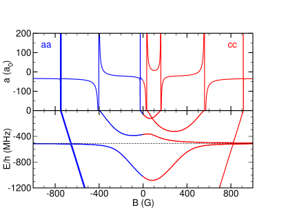
Figure S.2: Scattering length and $s$-wave bound state binding energies versus $B$ for channels $ii$ for $i=a,c$, where $E$ is relative to the channel energy $\epsilon_{ii}$ taken as 0. The dashed line shows where a pure van der Waals potential would have its last bound state with energy $E_{-1}$ for a scattering length of $a_{T}=-33.48\,a_{0}$ and the reduced mass of ³⁹K atoms.

There are several features that are evident from Fig. S.2. One is the changing spin character of the near-threshold bound states. Thus, unlike many other alkali species, there is no bound state in the low $B$-field region with the same magnetic moment as the $aa$ or the $cc$ entrance channels, as evidenced by the lack of an $E(B)$ curve parallel with the $E=0$ line. At high fields, $|B|\gtrsim 500\,$G, the magnetic Zeeman splitting exceeds the hyperfine splitting and a bound state with magnetic moment similar to that of the entrance channels emerges. This high field state takes on dominant triplet character and lies where one would expect the last $s$-wave bound state in a van der Waals potential with the triplet scattering length (see the dashed line in Fig. S.2).

Thus, the molecular states in the low field region where our experiment is performed do not have the entrance channel spin-character, but have a mixed character that is varying with $B$. This mixing is a consequence of the relatively small hyperfine coupling of ³⁹K and the presence of several $s$-wave bound states that mix. The relatively strong $B$-dependence of the atomic and molecular states is one of the main reasons we needed to construct an all-spin representation of the Efimov physics in order to properly describe the amplitude of three-body recombination.

The second feature that is evident from Fig. S.2 is the presence of overlapping resonances. These can not be described simply by a single pole formula Lange et al. (2009); Jachymski et al. (2013) of the conventional type,

$$a(B)=a_{\mathrm{bg}}\left(1-\frac{\Delta}{B-B_{0}}\right)\,,$$ (S3)

where $a_{\mathrm{bg}}$ is the $B$-independent background scattering length in the absence of a resonance and $\Delta$ represents the width of the resonance. Their product $a_{\mathrm{bg}}\Delta$ represents the “pole strength” of the resonance. The need for a two-pole fit is already known for the case of ³⁹K, since Roy et al. Roy et al. (2013) had to use a two-pole formula to represent their coupled channels results for the strongly overlapping $59.92\,$G and $65.67\,$G resonance features in the $bb$ spin channel ($|b\rangle=|F=1,M_{F}=0\rangle$) of ³⁹K. Consequently we fit our coupled channels $a(B)$ using a two-pole resonance expression similar to that of Ref. Roy et al. (2013) (note: Ref. Jachymski et al. (2013) showed this sum form is equivalent to the product form in Ref. Lange et al. (2009)):

$$a(B)=a_{\mathrm{bg}}^{g}\left(1-\frac{\Delta_{1}}{B-B_{0,1}}-\frac{\Delta_{2}}{B-B_{0,2}}\right)\,,$$ (S4)

where $a_{\mathrm{bg}}^{g}$ represents a “global” background for both resonances, which is not the same as that found from fitting a single pole. We obtain $a_{\mathrm{bg}}^{g}=$ $-19.599\,a_{0}$, widths $\Delta_{1}=54.772\,$G and $\Delta_{2}=-36.321\,$G, $B_{0,1}=B_{0}$ and the second resonance location at $B_{0,2}=162.341\,$G, consistent with the measured value $B_{0,2}=162.35(18)\,$G from Roy et al. Roy et al. (2013). Rewriting Eq. (S4) in the one-pole form of Eq. (S3) gives

$$a(B)=a_{\mathrm{bg}}^{\prime}\left(1+\delta(B)-\frac{\Delta^{\prime}}{B-B_{0}}\right)\,,$$ (S5)

where $a_{\mathrm{bg}}^{\prime}=a_{\mathrm{bg}}(1-\Delta_{2}/(B_{0,1}-B_{0,2}))=-14.070\,a_{0}$, $\Delta^{\prime}=\Delta(1-\Delta_{2}/(B_{0,1}-B_{0,2}))^{-1}=76.311\,$G, and $\delta(B)$ is a $B$-dependent correction that vanishes when $B=B_{0}$. A linear approximation for this case shows that $\delta(B)\approx-0.003052(B-B_{0,1})$, giving rise to a weak $B$-dependent background away from the pole. Clearly, by construction, the pole strength of the local pole at $B_{0}$, $a_{\mathrm{bg}}^{g}\Delta_{1}=a_{\mathrm{bg}}^{\prime}\Delta^{\prime}$ $=-1073.5\,a_{0}$G, is the same for either Eq. (S4) or (S5).

Finally, it should be noted that there is an alternative method to calculate the “pole strength” for decaying resonances like those in the $cc$ channel which are coupled through the magnetic dipole interaction to exit channel $d$-waves and can decay to lower energy open channels of the Zeeman manifold. We can use either the formulation of Hutson Hutson (2007) for the “resonance length” $a_{\mathrm{res}}$ of a decaying resonance with width $\delta$, or the equivalent formalism given for a decaying resonance by Nicholson et al. Nicholson et al. (2015).

In the Hutson formulation, $a_{\mathrm{res}}(\delta/2)=a_{\mathrm{bg}}\Delta$ Note (1), and the maximum variation in $a(B)$ is $\pm a_{\mathrm{res}}/2$ when the magnitude of the detuning from the pole is $|B-B_{0}|=\delta/2$. Using the MOLSCAT scattering code of Ref. Hutson and Le Sueur (2019) and a basis set including $s$ and $d$ partial waves, we calculate for the $34\,$G pole $a_{\mathrm{res}}=-2.1281\times 10^{7}\,a_{0}$ and $\delta=0.10084\,$mG, giving a pole strength of $-1073.0\,a_{0}$G; the same calculation determines “local” one-pole values of $a_{\mathrm{bg}}=-13.567\,a_{0}$ and $\Delta=78.975\,$G, giving the same product pole strength. This $a_{\mathrm{bg}}\Delta$ product is in good agreement with the value $-1073.5\,a_{0}$G calculated above from fitting a two-pole formula for $a(B)$ for the non-decaying resonances calculated with an $s$-wave basis only.

II.4 Determining the $s_{\mathrm{res}}$ parameter

Chin et al. Chin et al. (2010) defined a dimensionless parameter $s_{\mathrm{res}}$ to characterize Feshbach resonances when there is a long-range van der Waals potential. Although we never need to define this parameter to do our two-body coupled channels calculations or to set up and use our all-spin three-body calculations, we need to determine a value for it in making comparisons with other theories that make use of it.

As defined in Ref. Chin et al. (2010), the definition of $s_{\mathrm{res}}$ presumed a two-channel model of an isolated single resonance in which a single bound state in a closed channel is coupled to an open entrance channel:

$$s_{\mathrm{res}}=\frac{a_{\mathrm{bg}}\Delta}{\bar{a}}\frac{\delta\mu}{\bar{E}}\,,$$ (S6)

where $\bar{a}=(4\pi/\Gamma(\frac{1}{4})]^{2})\,r_{\mathrm{vdW}}\approx 0.955978\,r_{\mathrm{vdW}}\approx 61.77\,a_{0}$ Falke et al. (2008); Gribakin and Flambaum (1993) is related to the van der Waals length, $r_{\mathrm{vdW}}=\frac{1}{2}\left(mC_{6}/\hbar^{2}\right)^{\frac{1}{4}}\approx 64.61\,a_{0}$ for a van der Waals coefficient $C_{6}$ for the long-range potential; the corresponding energy scale is $\bar{E}=\hbar^{2}/(m\bar{a}^{2})$. The open entrance channel has a background scattering length $a_{\mathrm{bg}}$, and the closed channel state differs by $\delta\mu$ in magnetic moment from the total magnetic moment of the two individual atoms. The “bare” closed channel bound state is assumed to ramp linearly with slope $\delta\mu$ as the $B$ field is changed. The resonance coupling is characterized by the “pole strength” $a_{\mathrm{bg}}\Delta$ discussed in the last section. These approximations are adequate to characterize a wide variety of actual resonances involving various alkali-metal species.

The parameters $a_{\mathrm{bg}}$, $\Delta$, and $\delta\mu$ defining $s_{\mathrm{res}}$ in the model of Ref. Chin et al. (2010) were assumed to be independent of $B$-field tuning near the resonance. Thus, we will first attempt to estimate a plausible value for $\delta\mu$ using our full two-body coupled channels calculations of the bound states. Figure S.3 shows that a straight line with a slope of $\delta\mu/h=-2.52\,$MHz/G provides a good approximation to the bound state energy away from threshold to represent a ramping closed channel state. Using this value of the slope and subtracting it from the the slope of $0.91\,$MHz/G for the atomic threshold near the $34\,$G resonance (dashed line in Fig. S.3), along with the previously determined $a_{\mathrm{bg}}\Delta$ product determines a value of $s_{\mathrm{res}}\approx 2.45$. We note that the atomic magnetic moment near the $34\,$G resonance is still dependent on the $B$ field, which introduces some ambiguity on the value of $s_{\mathrm{res}}$ as defined in Eq. (S6). In our case, the value of $0.91\,$MHz/G is obtained by calculating the slope at $B=B_{0}$.

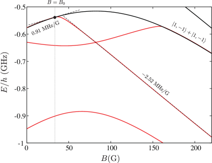
Figure S.3: Atomic (solid black) and calculated coupled channels bound state (solid red) absolute energies at different magnetic fields. The dashed lines with slopes of $0.91\,$MHz/G and $-2.52\,$MHz/G represent the atomic and molecular magnetic moments near and away from $B_{0}$ respectively; their difference is $\delta\mu/h\approx 3.43\,$MHz/G.

There are various approaches to extract the $s_{\mathrm{res}}$ value when $a_{\mathrm{bg}}$, the spin character or the magnetic moment varies across a resonance region. We follow the scheme based on the effective range similar to that discussed by Roy et al. Roy et al. (2013) (in their Supplemental Material) and Tanzi et al. Tanzi et al. (2018). We calculate the effective range $r_{e}$ from coupled channels calculations and use it to determine a value for $s_{\mathrm{res}}$. The effective range is the parameter that characterizes how the scattering properties vary with energy away from threshold. There is an analytic formula for $r_{e}$ for a two-channel representation of a local resonance in a van der Waals potential. It includes a term for a single channel with a van der Waals potential and a scattering length $a$, having the analytic form Gao (1998); Flambaum et al. (1999)

$$r_{e}^{(1)}(a)=\frac{\Gamma(\frac{1}{4})^{4}}{6\pi^{2}}\bar{a}\left(1-2\frac{\bar{a}}{a}+\left(\frac{\bar{a}}{a}\right)^{2}\right)\,,$$ (S7)

where the numerical factor $\Gamma(\frac{1}{4})^{4}/(6\pi^{2})\approx 2.91791$. The full two-channel expression also includes a resonant term depending on $s_{\mathrm{res}}$ and is given by Gao Gao (2011); also cited by Werner and Castin Werner and Castin (2012) as their Eq. (185), and is used in Refs. Roy et al. (2013); Tanzi et al. (2018):

$$r_{e}(B)=-2R^{*}\left(1-\frac{a_{\mathrm{bg}}}{a(B)}\right)^{2}+r_{e}^{(1)}(a(B))\,,$$ (S8)

where the parameter $R^{*}=\bar{a}/s_{\mathrm{res}}$. Using Eq. (S8) allows a value of $s_{\mathrm{res}}$ to be found from the knowledge of $r_{e}$ at the resonance pole position, where $a\to\infty$, and $r_{e}(B_{0})=-2\bar{a}/s_{\mathrm{res}}+2.91791\bar{a}$. Solving this latter expression for $s_{\mathrm{res}}$ given $r_{e}$ is trivial. Using our calculated value of $r_{e}(B_{0})\approx 133.91\,a_{0}$ at the $34\,$G resonance pole we obtain $s_{\mathrm{res}}\approx 2.68$ via this method.

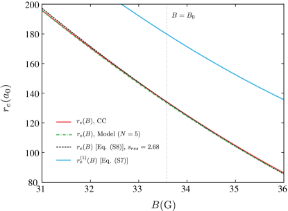
Figure S.4: Various calculations of the effective range $r_{e}$ versus $B$ for the $cc$ channel near the pole. The solid blue line is the single channel formula, Eq. (S7). The three nearly indistinguishable lines are: the solid red line for the full coupled channels (CC) result; the dashed line from formula Eq. (S8) for $s_{\mathrm{res}}\approx 2.68$; and the dot-dashed line calculated with our two-body reduced model described in Section III.2

Figure S.4 shows that the exact two-channel Eq. (S8) gives an excellent approximation to the true coupled channels result for $r_{e}(B)$ when $s_{\mathrm{res}}\approx\>2.68$. Figure S.4 also shows that the values of $r_{e}(B)$ determined by our reduced two-body model (with $N=5$ singlet bound states), used in our three-body calculations and described in Section III.2, are also nearly indistinguishable from the coupled channels calculations. We note that the value $s_{\mathrm{res}}\approx 2.68$ is also consistent with the $s_{\mathrm{res}}\approx 2.45$ obtained from the analysis of the magnetic moment $\delta\mu$. Therefore, we will take the arithmetic mean 2.57 as the best value for $s_{\mathrm{res}}$.

Finally, we comment that it can be a useful heuristic to think of $s_{\mathrm{res}}$ as defining the width of the Feshbach resonance’s universal region. For sufficiently small positive magnetic field detunings $\delta_{B}=B-B_{0}$, the bound state is fully in the open channel, where the binding energy and the scattering length follow the universal expressions $E_{b}\approx\hbar^{2}/(ma^{2})$ and $a(B)\approx a_{\mathrm{bg}}\Delta/\delta_{B}$, such that $\partial E_{b}/\partial\delta_{B}\approx 2(\hbar^{2}/m)\delta_{B}/(a_{\mathrm{bg}}\Delta)^{2}$. At large values of $\delta_{B}$, the bound state asymptotes to the closed channel and $\partial E_{b}/\partial\delta_{B}\approx\delta\mu$. We can define a crossover scattering length $a_{c}$ for which the open-channel prediction for $\partial E_{b}/\partial\delta_{B}$ is half of the ultimate asymptotic limit. For $s_{\mathrm{res}}\lesssim 1$ and $|a_{\mathrm{bg}}|\lesssim r_{\mathrm{vdW}}$, we might then expect more open-channel, universal behavior when $a\gg a_{c}\approx 4r_{\mathrm{vdW}}/s_{\mathrm{res}}$.

Table 2: Efimov resonance measurement conditions and fit results. We extract the Efimov peak location, width and height from the zero-temperature Eq. (1), limiting fits to data points for which $\left|a\right|<\lambda/10$. We extract $a_{-}$, $\eta$ and $A$ from the finite-temperature Eq. (2).

$\bar{T}$	$T_{\mathrm{i}}$	$\langle n\rangle_{\mathrm{i}}$	$\bar{\omega}/2\pi$	peak location	peak width	peak height	$a_{-}$	$\eta$	A
nK	nK	$10^{11}\thinspace\mathrm{cm^{-3}}$	Hz	$-a_{0}$			$-a_{0}$
$30$	$27$	$0.40$	$33.7$	$891(8)$	$0.22(1)$	1.29(4)	910(9)	0.24(1)	1.40(4)
$53$	$46$	$0.70$	$40.8$	$856(10)$	$0.22(1)$	1.28(5)	904(12)	0.24(1)	1.43(6)
$94$	$85$	$1.07$	$51.4$	$829(7)$	$0.24(1)$	0.92(3)	890(7)	0.24(1)	1.08(2)
$206$	$186$	$1.21$	$65.7$	$807(14)$	$0.30(2)$	0.65(3)	921(6)	0.25(1)	0.91(1)
$510$	$407$	$3.52$	$89.9$	$811(46)$	$0.44(3)$	0.54(5)	917(9)	0.26(1)	0.89(1)
$173$	$160$	$2.18$	$51.1$
$221$	$194$	$8.76$	$51.1$

III Efimov Resonance Location

III.1 Data Conditions and Fit Results

A compilation of Efimov resonance measurement conditions and fit results is presented in Table LABEL:table:Efimov_table. Each temperature data set is described by a time-averaged temperature $\bar{T}$, initial temperature $T_{\mathrm{i}}$, initial mean density $\langle n\rangle_{\mathrm{i}}$ and a mean trap frequency $\bar{\omega}$. Atom number and temperature at each interrogation time are extracted from absorption images of the sample after a fixed time-of-flight, assuming Maxwell-Boltzmann distribution of the sample. Trapping frequencies are measured using the slosh motion of the sample along two orthogonal directions. Efimov $L_{3}/a^{4}$ peak locations, widths and heights are determined from fits to the zero-temperature zero-range expression (Eq. (1) of the main text), limiting fits to data points for which $\left|a\right|<\lambda/10$ (thermal wavelength) and redefining $a_{-}$ as the peak location, $\eta$ as the peak width and the fit prefactor as the peak height. We extract the true Efimov ground state location $a_{-}$ and $\eta$ from a fit to the finite-temperature zero-range expression (Eq. (2) of the main text), where the fit amplitude prefactor deviation from unity describes the uncertainty in our absolute density calibration. We do not include fit results for high $na^{3}$ data, for which there appears to be some unaccounted for many-body effect.

III.2 Three-body Coupled-Channel Model

Our three-body calculations for ³⁹K atoms were performed using the adiabatic hyperspherical representation Suno et al. (2002); Wang et al. (2011, 2012a, 2012b); Mestrom et al. (2017), with atoms containing the proper hyperfine structure. In order to incorporate such effects we have used Feshbach projectors in an approach similar to the one used in Ref. Jonsell (2004). In the hyperspherical representation the hyperradius $R$ determines the overall size of the system, while all other degrees of freedom are represented by a set of hyperangles $\Omega$. Within this framework, the three-body adiabatic potentials $U$ and channel functions $\Phi$ are determined from the solutions of the hyperangular adiabatic equation:

$$\left[\frac{\Lambda^{2}(\Omega)+15/4}{2\mu R^{2}}\hbar^{2}+\varepsilon_{\alpha}\right]\Phi_{\alpha}(R;\Omega)$$

$$+\sum_{\beta}\sum_{i<j}V_{\alpha\beta}(r_{ij})\Phi_{\beta}(R;\Omega)=U(R)\Phi_{\alpha}(R;\Omega)\,.$$ (S9)

This expression contains the hyperangular part of the kinetic energy, expressed through the grand-angular momentum operator $\Lambda^{2}$ and the three-body reduced mass $\mu=m/\sqrt{3}$. In our formulation, as well as that of Ref. Jonsell (2004), the multichannel structure of interatomic interactions uses the same two-body interaction potentials as in Eq. S2. The resonant spin channels we consider are fully symmetric with $m_{F_{1}}+m_{F_{2}}+m_{F_{3}}=-3$, with at least one pair, $ij$, with $m_{F_{i}}+m_{F_{j}}=-2$ and the third, $k$, atom in the $|F_{k}=1,m_{F_{k}}=-1\rangle$ state. We note that, since our interaction model incorporates the proper hyperfine structure, as well as singlet and triplet interactions, the correct values of all two-body resonance parameters, including $s_{\mathrm{res}}$ and $a_{\mathrm{bg}}$, are naturally built in.

For our three-body calculations near the $B_{0}=33.5820\,$G resonance, we have replaced the actual singlet and triplet potentials from Ref. Falke et al. (2008) by two Lennard-Jones potentials, $v_{S}(r)=-C_{6}/r^{6}(1-\lambda_{S}^{6}/r^{6})$, and $v_{T}(r)=-C_{6}/r^{6}(1-\lambda_{T}^{6}/r^{6})$, with $\lambda_{S}$ and $\lambda_{T}$ adjusted to correctly produce the singlet and triplet scattering lengths but with a much smaller number of bound states than the real interactions. In practice, we allowed in our model for small variations in $a_{S}$ and $a_{T}$ to fine tune the background scattering length $a_{\mathrm{bg}}$ and width of the Feshbach resonance, $\Delta$, thus ensuring the proper pole strength $a_{\mathrm{bg}}\Delta$. The fact that we are replacing the realistic singlet and triplet potentials but preserving the atomic hyperfine interactions eliminates the necessity to specify the value of $s_{\mathrm{res}}$, while still accurately describing the properties of the Feshbach resonance (see Fig. S.4). Moreover, our reduced model has the correct mixing of the spin states and thus properly describes the relevant molecular channels for three-body recombination. These aspects, absent in most previous three-body models Schmidt et al. (2012); Wang and Julienne (2014); Langmack et al. (2018), are important for the low $B$-field Feshbach resonances in ³⁹K, where the $B$-field dependence of the hyperfine interactions leads to a strongly mixed spin character of both atomic and molecular states.

The value for the Efimov resonance position $a_{-}$ is obtained using $v_{S}$ and $v_{T}$ potentials supporting different numbers of $s$-wave bound states. This is done by solving the hyperradial Schrödinger equation Wang et al. (2011),

$$\left[-\frac{\hbar^{2}}{2\mu}\frac{d^{2}}{dR^{2}}+U_{\nu}(R)\right]F_{\nu}(R)$$

$$~{}~{}~{}~{}~{}~{}+\sum_{\nu^{\prime}}W_{\nu\nu^{\prime}}(R)F_{\nu^{\prime}}(R)=EF_{\nu}(R)\,,$$ (S10)

where $\nu$ is an index that labels all necessary quantum numbers to characterize each channel, and $E$ is the total energy. From the above equation we determine the scattering $S$-matrix, and the resulting recombination rate $L_{3}$. The value for $a_{-}$, as well as the inelasticity parameter $\eta$, are then determined via fitting to the universal formula Eq. (1) of the main text. The predicted values for $a_{-}$ and $\eta$ are listed in Table 3 for different numbers of $s$-wave singlet bound states $N_{S}\equiv N$ our model potential can support. The number of triplet $s$-wave states is given by $N_{T}=N-1$. We also list the total number of bound states in Table 3, including all partial waves, after adding the hyperfine interactions that cause the mixing between singlet and triplet states.

From Table 3 we see a considerable dependence of $a_{-}$ on the number of $s$-wave states approaching a limiting value that differs only $8\%$ from the experimental finding of $a_{-}=-14.05(17)\,r_{\rm vdW}$. This stronger dependence on the number of bound states is in contrast to the results obtained for broad resonances Wang et al. (2012a). We also see a similar behavior for the inelasticity parameter $\eta$, whose limiting value is 0.21. This remarkable level of agreement for $\eta$ indicates that our model is capable of properly describing the reaction rates in the system. Given our assumption that the pairwise additive long-range potentials are sufficient to account for the Efimov physics, our three-body model should be valid for $B$-fields in which the two-body bound states and scattering properties are described properly. Possible future improvements in our three-body model would include the effects of the magnetic-dipole interactions that couple $s$- and $d$-wave two-body interactions, a more realistic model of electronic exchange interactions, and checking the effect of non-additive short-range three-body potentials.

Table 3: Values for the three-body parameter $a_{-}$ and inelasticity parameter $\eta$ as a function of singlet number of $s$-wave bound states $N_{S}\equiv N$ (or the total number of bound states $N_{\mathrm{tot}}$ including those of nonvanishing rotational angular momenta). We extrapolate to high-$N$ by fitting to different functional forms and take the fit results spread as the uncertainty for the limiting $a_{-}$ and $\eta$ values. The last row lists experimental results obtained in the present work.

$N$	$N_{\mathrm{tot}}$	$a_{-}/r_{\rm vdW}$	$\eta$
2	6	$-7.61$	0.10
3	27	$-11.20$	0.19
4	59	$-12.27$	0.20
5	105	$-12.69$	0.21
$\vdots$	$\vdots$	$\vdots$	$\vdots$
$\infty$	$\infty$	$-13.1(3)$	0.21(1)
Exp.		$-14.05(17)$	0.25(1)

References

- Chin et al. (2010) C. Chin, R. Grimm, P. Julienne, and E. Tiesinga, Rev. Mod. Phys. 82, 1225 (2010).
- Falke et al. (2008) S. Falke, H. Knöckel, J. Friebe, M. Riedmann, E. Tiemann, and C. Lisdat, Phys. Rev. A 78, 012503 (2008).
- Wang et al. (2011) J. Wang, J. P. D’Incao, and C. H. Greene, Phys. Rev. A 84, 052721 (2011).
- Wang et al. (2012a) J. Wang, J. P. D’Incao, B. D. Esry, and C. H. Greene, Phys. Rev. Lett. 108, 263001 (2012a).
- Wang et al. (2012b) Y. Wang, J. Wang, J. P. D’Incao, and C. H. Greene, Phys. Rev. Lett. 109, 243201 (2012b).
- Mestrom et al. (2017) P. M. A. Mestrom, J. Wang, C. H. Greene, and J. P. D’Incao, Phys. Rev. A 95, 032707 (2017).
- Suno et al. (2002) H. Suno, B. D. Esry, C. H. Greene, and J. P. Burke, Phys. Rev. A 65, 042725 (2002).
- Chin and Julienne (2005) C. Chin and P. S. Julienne, Phys. Rev. A 71, 012713 (2005).
- Idziaszek and Calarco (2006) Z. Idziaszek and T. Calarco, Phys. Rev. A 74, 022712 (2006).
- Stoof et al. (1988) H. T. C. Stoof, J. M. V. A. Koelman, and B. J. Verhaar, Phys. Rev. B 38, 4688 (1988).
- Tiesinga et al. (2000) E. Tiesinga, C. J. Williams, F. H. Mies, and P. S. Julienne, Phys. Rev. A 61, 063416 (2000).
- Roy et al. (2013) S. Roy, M. Landini, A. Trenkwalder, G. Semeghini, G. Spagnolli, A. Simoni, M. Fattori, M. Inguscio, and G. Modugno, Phys. Rev. Lett. 111, 053202 (2013).
- D’Errico et al. (2007) C. D’Errico, M. Zaccanti, M. Fattori, G. Roati, M. Inguscio, G. Modugno, and A. Simoni, New Journal of Physics 9, 223 (2007).
- Berninger et al. (2013) M. Berninger, A. Zenesini, B. Huang, W. Harm, H.-C. Nägerl, F. Ferlaino, R. Grimm, P. S. Julienne, and J. M. Hutson, Phys. Rev. A 87, 032517 (2013).
- Lange et al. (2009) A. D. Lange, K. Pilch, A. Prantner, F. Ferlaino, B. Engeser, H.-C. Nägerl, R. Grimm, and C. Chin, Phys. Rev. A 79, 013622 (2009).
- Jachymski et al. (2013) K. Jachymski, M. Krych, P. S. Julienne, and Z. Idziaszek, Phys. Rev. Lett. 110, 213202 (2013).
- Hutson (2007) J. M. Hutson, New Journal of Physics 9, 152 (2007).
- Nicholson et al. (2015) T. L. Nicholson, S. Blatt, B. J. Bloom, J. R. Williams, J. W. Thomsen, J. Ye, and P. S. Julienne, Phys. Rev. A 92, 022709 (2015).
- Note (1) Note that the definition of in Hutson Hutson (2007) is twice the value defined by Eq. (26) of Chin et al. Chin et al. (2010).
- Hutson and Le Sueur (2019) J. M. Hutson and C. R. Le Sueur, Computer Physics Communications 241, 9 (2019).
- Gribakin and Flambaum (1993) G. F. Gribakin and V. V. Flambaum, Phys. Rev. A 48, 546 (1993).
- Tanzi et al. (2018) L. Tanzi, C. R. Cabrera, J. Sanz, P. Cheiney, M. Tomza, and L. Tarruell, Phys. Rev. A 98, 062712 (2018).
- Gao (1998) B. Gao, Phys. Rev. A 58, 1728 (1998).
- Flambaum et al. (1999) V. V. Flambaum, G. F. Gribakin, and C. Harabati, Phys. Rev. A 59, 1998 (1999).
- Gao (2011) B. Gao, Phys. Rev. A 84, 022706 (2011).
- Werner and Castin (2012) F. Werner and Y. Castin, Phys. Rev. A 86, 013626 (2012).
- Jonsell (2004) S. Jonsell, Journal of Physics B: Atomic, Molecular and Optical Physics 37, S245 (2004).
- Schmidt et al. (2012) R. Schmidt, S. P. Rath, and W. Zwerger, Eur. Phys. J. B 85, 386 (2012).
- Wang and Julienne (2014) Y. Wang and P. S. Julienne, Nat. Phys. 10, 768 (2014).
- Langmack et al. (2018) C. Langmack, R. Schmidt, and W. Zwerger, Phys. Rev. A 97, 033623 (2018).