Analyses of Multi-collection Corpora via Compound Topic Modeling

Abstract

As electronically stored data grow in daily life, obtaining novel and relevant information becomes challenging in text mining. Thus people have sought statistical methods based on term frequency, matrix algebra, or topic modeling for text mining. Popular topic models have centered on one single text collection, which is deficient for comparative text analyses. We consider a setting where one can partition the corpus into subcollections. Each subcollection shares a common set of topics, but there exists relative variation in topic proportions among collections. Including any prior knowledge about the corpus (e.g. organization structure), we propose the compound latent Dirichlet allocation (cLDA) model, improving on previous work, encouraging generalizability, and depending less on user-input parameters. To identify the parameters of interest in cLDA, we study Markov chain Monte Carlo (MCMC) and variational inference approaches extensively, and suggest an efficient MCMC method. We evaluate cLDA qualitatively and quantitatively using both synthetic and real-world corpora. The usability study on some real-world corpora illustrates the superiority of cLDA to explore the underlying topics automatically but also model their connections and variations across multiple collections.

Keywords— Statistical learning, Unsupervised learning, Text analysis, Topic models

1 Introduction

Newspapers, magazines, scientific journals, and social media messages being composed in daily living produce routinely an enormous volume of text data. The corresponding content comes from diverse backgrounds and represent distinct themes or ideas; modeling and analyzing such heterogeneity in large-scale is crucial in any text mining frameworks. Typically, text mining aims to extract relevant and interesting information from the text by the process of structuring the written text (e.g. via semantic parsing, stemming, lemmatization), inferring hidden patterns within the structured data, and finally, deciphering the results. To address these tasks in an unsupervised manner, numerous statistical methods such as TF-IDF (Salton et al., 1975), latent semantic indexing (Deerwester et al., 1990, LSI), and probabilistic topic models, e.g. probabilistic LSI (Hofmann, 1999, pLSI), latent Dirichlet allocation (Blei et al., 2003, LDA), have emerged in the literature. With minimal human effort, they can be generalized to arbitrary text in any natural language.

Topic models such as LDA are developed to capture the underlying semantic structure of a corpus (i.e. a document collection) based on co-occurrences of words. They consider documents as bags of words, considering the order of words in a document uninformative. LDA (Figure 2) assumes that (a) a topic is a latent (i.e., unobserved) distribution on the corpus vocabulary, (b) each document in the corpus is described by a latent mixture of topics, and (c) each observed word in a document, there is a latent variable representing a topic from which the word is drawn. This model is suitable for documents coming from a single collection. This assumption is insufficient for comparative analyses of text, especially, for partition-able text corpora, as we describe next.

Suppose, we deal with corpora of (i) articles accepted in various workshops or consecutive proceedings of a conference or (ii) blogs/forums from people different countries. It may be of interest to explore research topics across multiple/consecutive proceedings or workshops of a conference or cultural differences in blogs and forums from different countries (Zhai et al., 2004). Suppose, we have political news articles from different sources such as New York Times, Washington Post, The Wall Street Journal, and Reuters. Although, all talk about topic politics, modeling articles from each news source as a collection may help to explore each sources’ article style, policies, region influences, culture, etc. Moreover, the category labels, workshop names, article timestamps, or geotags can provide significant prior knowledge regarding the unique structure of these corpora. We aim to include these prior structures and characteristics of the corpus into a probabilistic model adding less computational burden, for expert analyses of the corpus, collection, and document-level characteristics.

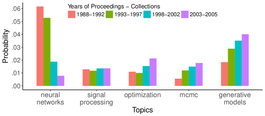
Figure 1: Estimated topic proportions of five topics for the four time spans of the NIPS conference proceedings.

For example, Figure 1 gives the results of an experiment on a real document corpus employing the proposed model in this paper. The corpus consists of articles accepted in the proceedings of the NIPS conference for the years from $1988$ to $2005$. We wish to analyze topics that evolve over this timespan. We thus partitioned the corpus into four collections based on time (details in Section 4). The plot shows estimates of topic proportions for all four collections. Evidently, some topics got increased attention (e.g. Markov chain Monte Carlo (MCMC), generative models) and some topics got decreased popularity (e.g. neural networks) over the years of the conference. For some topics, the popularity is relatively constant (e.g. signal processing) from the beginning of NIPS. The algorithm used is unsupervised, and only takes documents, words, and their collection labels as input.

Assuming a flat structure to all documents in a corpus, LDA or its variants is not well suited to the multi-collection corpora setting: (1) Ignoring predefined structure or organization of collections may end up having topics that describe only some, not all of the collections. (2) There is no direct way to define which set of topics describe the common information across collections and which topic describes information specific to a particular collection. A crude solution is to consider each collection as a separate corpus and fit an LDA model for each corpus. There are reasons why one may want to avoid it: (i) one needs to solve the nontrivial alignment of topics in each model, for any useful comparison of topics among collections (Moreover, the topics inferred from individual corpus partitions and the whole corpora can themselves be different) and (ii) information loss due to modeling collections separately, especially for small datasets (details, Section 4.2).

In this paper, we introduce the compound latent Dirichlet allocation (cLDA, Section 2) model that incorporates any prior knowledge on the organization of documents in a corpus into a unified modeling framework. cLDA assumes a shared, collection-level, latent mixture of topics for documents in each collection. This collection-level mixture is used as the base measure to derive the (latent) topic mixture for each document. All collection-level and document-level variables share a common set of topics at the corpus level, which enables us to perform exciting inferences, as shown in Figure 1. cLDA exhibits a certain degree of supervision incorporating the collection membership for each word (and document) in a corpus implicitly in the modeling framework. cLDA can thus aid visual thematic analyses of large sets of documents, and include corpus, collection, and document specific views.

The parameters of interest in cLDA are hidden and are inferred via posterior inference. However, exact inference is intractable in cLDA; and, non-conjugate relationships in the model further make approximate inference challenging. Popular approximate posterior inference methods in topic models are MCMC and variational methods. MCMC methods enable us to sample hidden variables of interest from the intractable posterior with convergence guarantees. We consider two MCMC methods for cLDA: (a) one uses the traditional auxiliary variable updates within Gibbs sampling, and (b) the other uses Langevin dynamics within Gibbs sampling, a method that received recent attention. Our experimental evidence suggests the former method, which gives superior performance with only a little computational overhead compared to the collapsed Gibbs sampling algorithm for LDA (Griffiths and Steyvers, 2004, CGS) (details in Sections 3.2, 4, F, and H), and is the main focus in this paper. Variational methods are often used in topic modeling as they give fast, parallel implementations by construction. Although they converge rather quickly, our studies show that (Section 3.2 and Section F) their solutions are suboptimal compared to the results of the other two MCMC schemes.

The contributions of this paper are three-fold: (i) we propose a probabilistic model cLDA that can capture the topic structure of a corpus including organization hierarchy of documents, (ii) we study efficient methods for posterior inference in cLDA, and (iii) we perform an empirical study of the real-world applicability of the cLDA model—for example, (a) analyzing topics that evolves overtime, (b) analyzing patterns of topics on customer reviews, and (a) summarizing topic structure of document collections in a corpus—via three text corpora used in the research community. Also, note that the inference about collection-level topic mixtures may be of interest to the general perspective of posterior sampling on the probability simplex in statistics.

The remainder of the paper is organized as follows. Section 2 formally defines the cLDA hierarchical model. Section 3 describes algorithms for posterior inference and evaluates correctness of the algorithms using a synthetically corpus. In Section 4, we assess the performance of the cLDA model and conclude that it exhibits superior performance, both quantitatively (e.g. via perplexity—a popular scheme for evaluating the predictive performance of topic models (Wallach et al., 2009b), and external measures such as topic coherence (Mimno et al., 2011)) and qualitatively. We also compare cLDA with other popular models in the literature, and provide a usability study for cLDA in this section. Section 5 concludes this paper with a summary of our work.

2 A Compound Hierarchical Model

We first set up some terminology and notation. Vectors are denoted by bold, lower case alphabets (e.g. $\bm{\pi}$) and scalar values are denoted by normal, lowercase letters (e.g. $\pi_{jk}$). Matrices or tensors are denoted by bold, upper case Latin alphabets (e.g. ${\bm{G}}$) or bold Greek alphabets without subscripts (e.g. $\bm{\beta}$). There is a vocabulary $\mathcal{V}$ of $V$ terms in the corpus; in general, $\mathcal{V}$ is considered as the union of all the word tokens in all the documents of the corpus, after removing stop-words and normalizing tokens (e.g. stemming). The number of topics $K$ is assumed to be known. (Discussion of how to handle this issue in practice is Section 4.) By definition, a topic is a distribution over ${\cal V}$, i.e., a point in the $V$-$1$ dimensional simplex $\mathbb{S}_{V}$. We will form a $K\times V$ matrix $\bm{\beta}$, whose $k^{\text{th}}$ row is the $k^{\text{th}}$ topic (how $\bm{\beta}$ is formed will be described shortly). Thus, the rows of $\bm{\beta}$ are vectors $\bm{\beta}_{1},\ldots,\bm{\beta}_{K}$, all lying in $\mathbb{S}_{V}$. There are $J$ collections in the corpus and for $j=1,2,\ldots,J$, collection $j$ has $D_{j}$ documents. For $d=1,\ldots,D_{j}$, document $d$ in collection $j$ (i.e. document $jd$) has $n_{jd}$ words, $w_{jd1},\ldots,w_{jdn_{jd}}$. Each word is represented by the index or id of the corresponding term from the vocabulary. We represent document $jd$ by the vector ${\bm{w}}_{jd}=(w_{jd1},\ldots,w_{jdn_{jd}})$, collection $j$ by the concatenated vector ${\bm{w}}_{j}=({\bm{w}}_{j1},\ldots,{\bm{w}}_{jD_{j}})$, and the corpus by the concatenated vector ${\bm{w}}=({\bm{w}}_{1},\ldots,{\bm{w}}_{J})$.

Figure 2: Graphical model of the latent Dirichlet allocation (LDA) model (the inner structure) and the compound latent Dirichlet allocation (cLDA) model (the outer dashed-structure is the extension to LDA): Nodes denote random variables, shaded nodes denote observed variables, edges denote conditional dependencies, and plates denote replicated processes.

We use $\operatorname{Dir}_{L}(a\omega_{1},\ldots,a\omega_{L})$ to denote the finite-dimensional Dirichlet distribution on the ($L$-$1$)-dimensional simplex. This has two parameters, a scale (concentration) parameter $a$ and a base measure $(\omega_{1},\ldots,\omega_{L})$ on the ($L$-$1$)-dimensional simplex. Thus $\operatorname{Dir}_{L}(a,\ldots,a)$ denotes an $L$-dimensional Dirichlet distribution with the constant base measure $(1,\ldots,1)$. $\operatorname{Mult}_{L}(b_{1},\ldots,b_{L})$ to represents the multinomial distribution with number of trials equal to $1$ and probability vector $(b_{1},\ldots,b_{L})$. Let $h=(\eta,\alpha,\gamma)\in(0,\infty)^{3}$ be the hyperparameters in the model. We formally define the cLDA model as (see Figure 2).

$$\bm{\beta}_{k} \stackrel{{\scriptstyle\text{iid}}}{{\sim}} \operatorname{Dir}_{V}(\eta,\ldots,\eta),\text{ for topic }k=1,\ldots,K$$ (1)

$$\bm{\pi}_{j} \stackrel{{\scriptstyle\text{iid}}}{{\sim}} \operatorname{Dir}_{K}(\alpha,\ldots,\alpha),\text{ for collection }j=1,\ldots,J$$ (2)

$$\bm{\theta}_{jd} \stackrel{{\scriptstyle\text{iid}}}{{\sim}} \operatorname{Dir}_{K}(\gamma\pi_{j1},\ldots,\gamma\pi_{jK}),\text{ for document }jd$$ (3)

$$z_{jdi} \stackrel{{\scriptstyle\text{iid}}}{{\sim}} \operatorname{Mult}_{K}(\bm{\theta}_{jd}),\text{ for each word }w_{jdi}$$ (4)

$$w_{jdi} \stackrel{{\scriptstyle\text{ind}}}{{\sim}} \operatorname{Mult}_{V}(\bm{\beta}_{z_{jdi}})$$ (5)

The distribution of $z_{jd1},\ldots,z_{jdn_{jd}}$ will depend on the document-level variable $\bm{\theta}_{jd}$ that represents a distribution on the topics for document $jd$. A single $\bm{\theta}_{jd}$ for document $jd$ encourages different words in document $jd$ to share the same document level characteristics. The distribution of $\bm{\theta}_{j1},\ldots,\bm{\theta}_{jD_{j}}$ will depend on the collection-level variable $\bm{\pi}_{j}$ which indicates a distribution on the topics for collection $j$. A single $\bm{\pi}_{j}$ for collection $j$ encourages different documents in collection $j$ to have the same collection level properties. A single $\bm{\beta}$ is shared among all documents, which encourages documents in various collections in the corpus to share the same set of topics. Note that the standard LDA model (Blei et al., 2003) is a special case of the proposed cLDA model, where there exist single parameters $\bm{\pi}_{j}$ and $\bm{\beta}$ that fail to capture potential heterogeneity amongst the predefined collections, an objective that cLDA is designed for.

Related Work

Zhai et al. (2004) refer to the problem of multi-collection corpora modeling as comparative text mining (CTM), which uses pLSI as a building block. Comparing with CTM model, cLDA employs an efficient and generalizable LDA-based framework that has several advantages over pLSI—for example, LDA incorporates Dirichlet priors for document topic structures in a natural way to deal with newly encountered documents. Furthermore, cLDA combines collection-specific characteristics in a natural probabilistic framework enabling efficient posterior sampling, depending less on user-defined parameters as in CTM.

The cLDA model shares some similarities, but also exhibits differences from: Hierarchical Dirichlet Process (Teh et al., 2006) and Nested Chinese Restaurant Process (Blei et al., 2004), which are introduced to learn document and topic hierarchies from the data non-parametrically. In nonparametric models, as we observe more and more data, the data representations grow structurally. Instead of manually specifying the number of topics K, these nonparametric topic models infer K from the data by assuming a Dirichlet process prior for document topic distributions and topics. A major hurdle in these frameworks is that inference can be computationally challenging for large datasets. Our experimental evidence also shows that HDP produces too many fragmented topics, which may lead the practitioner to bear the additional burden of post processing (Section 4.2). Here, similar to LDA, cLDA is a parametric model, i.e., the data representational structure is fixed and does not grow as more data are observed. cLDA assumes that K is fixed and can be inferred from the data directly, e.g., empirical Bayes methods (George, 2015), or by cross-validation. We thus have simple Dirichlet priors in cLDA without adding much burden to the model and inference (details appear in Section 3).

In light of adding supervision, several modifications to LDA model have been proposed in the literature. Supervised LDA (Mcauliffe and Blei, 2008, sLDA) is an example; for each document $d$, sLDA introduces a response variable $y_{d}$ that is assumed to be generated from document $d$’s empirical topic mixture distribution. In practice, the posterior inference in such a setting can be inefficient due to the high non-linearity of the discrete distribution on the empirical parameters (Zhu and Xing, 2014). cLDA, on the other hand, proposes a generative framework incorporating the collection-level characteristics, without much computational burden (details, Section 4). Also, the objectives of these related models are different from the focus of this paper.

One can view the hierarchical model of cLDA as a special instance of the model proposed by Kim et al. (2013). Kim et al. (2013) extended the LDA model to have multiple layers in the hierarchical model, for corpora with many categories and subcategories. In cLDA, we are interested in corpora with just one layer of top level categories. This model is adequate for many real-world corpora such as books with various chapters and conference proceedings from different years. Additionally, we will show that Kim et al. (2013)’s variational methods for the multilayer hierarchical model is suboptimal compared to the proposed MCMC methods for two layered data.

A popular scheme for evaluating the performance of topic models is perplexity (or the predictive probability of held-out documents), which we use here to assess cLDA’s performance quantitatively. In the text domain, one can use trained cLDA models for tasks such as classifying text documents and summarizing document collections and corpora. cLDA also gives excellent options to visualize and browse documents. The model and algorithm we describe can be used to form a hierarchy of documents in a collection including relevant topic information. One can then use the document hierarchy to enlighten one’s perception of the contents of the collection.

3 Posterior Sampling

The parameters of interest in the cLDA model, i.e., (a) corpus-level topics, (b) collection-level mixture of topics, (c) document-level mixture of topics, and (d) topic indices of words are hidden. We identify these hidden variables given the observed word statistics and document organization hierarchy in the corpus via posterior inference.

Let $\bm{\theta}=(\bm{\theta}_{11},\ldots,\bm{\theta}_{1D_{1}},\ldots,\bm{\theta}_{J1},\ldots,\bm{\theta}_{JD_{J}})$, ${\bm{z}}_{jd}=(z_{jd1},\ldots,z_{jdn_{jd}})$ for $d=1,\ldots,D_{j}$, $j=1,\ldots,J$, ${\bm{z}}=({\bm{z}}_{11},\ldots,{\bm{z}}_{1D_{1}},\ldots,{\bm{z}}_{J1},\ldots,{\bm{z}}_{JD_{J}})$, and $\bm{\pi}=(\bm{\pi}_{1},\ldots,\bm{\pi}_{J})$. We will then use $\bm{\psi}$ to denote the latent variables $(\bm{\beta},\bm{\pi},\bm{\theta},{\bm{z}})$ in the cLDA model. For any given $h$, (1)–(5) in the hierarchical model induce a prior distribution $p_{h}(\bm{\psi})$ on $\bm{\psi}$. Equation (5) gives the likelihood $\ell_{{\bm{w}}}(\bm{\psi})$. The words ${\bm{w}}$ and their document and collection labels are observed. We are interested in $p_{h,{\bm{w}}}(\bm{\psi})$, the posterior distribution of $\bm{\psi}$ given ${\bm{w}}$ corresponding to the prior $p_{h}(\bm{\psi})$. Applying Bayes rule, we can write the posterior distribution $p_{h,{\bm{w}}}$ of $\bm{\psi}$ as

$$p_{h,{\bm{w}}}(\bm{\psi})\propto\ell_{{\bm{w}}}(\bm{\psi})p_{h}(\bm{\psi})\\$$ (6)

Using (1)–(5) of the hierarchical model, we can write (6) as (Section A gives additional details)

$$\begin{split}p_{h,{\bm{w}}}(\bm{\psi})&\propto\Biggl{[}\prod_{j=1}^{J}\prod_{d=1}^{D_{j}}\frac{\prod_{k=1}^{K}\theta_{jdk}^{n_{jdk}+\gamma\pi_{jk}-1}}{\prod_{k=1}^{K}{\Gamma(\gamma\pi_{jk})}}\Biggr{]}\Biggl{[}\prod_{j=1}^{J}\prod_{k=1}^{K}\pi_{jk}^{\alpha-1}\Biggr{]}\\ &\hskip 14.22636pt\Biggl{[}\prod_{k=1}^{K}\prod_{v=1}^{V}\beta_{kv}^{\sum_{j=1}^{J}\sum_{d=1}^{D_{j}}m_{jdkv}+\eta-1}\Biggr{]}\end{split}$$ (7)

where $n_{jdk}$ is the number of words in document $d$ in collection $j$ that are assigned to topic $k$, and $m_{jdkv}$ is the number of words in document $d$ in collection $j$ for which the latent topic is $k$ and the index of the word in the vocabulary is $v$. These count statistics depend on both ${\bm{z}}$ and ${\bm{w}}$. Note that the constants in the Dirichlet normalizing constants are absorbed into the overall constant of proportionality. Unfortunately, the normalizing constant of the posterior $p_{h,{\bm{w}}}(\bm{\psi})$, is the likelihood of the data with all latent variables integrated out, is a non-trivial integral. This makes exact inference difficult in cLDA.

Popular methods for approximate posterior inference in topic models are Markov chain Monte Carlo (e.g. see Griffiths and Steyvers (2004)) and variational methods (e.g. see Blei et al. (2003)). Although variational methods may give a fast and scalable approximation for the posterior, due to optimizing the proxy lower-bound, it may not produce optimal solutions as the MCMC methods in practice (e.g. see Teh et al. (2007)). That is the case in this model setting, as our experimental evidence suggests. Hence, we leave the details of our development of variational methods (VEM) for cLDA in Section E, to stay our discussion focused.

3.1 Inference via Markov chain Monte Carlo Methods

According to the hierarchical model (1)–(5), $\bm{\theta}_{jd}$’s and $\bm{\beta}_{k}$’s are independent, and by inspecting the posterior (6), given $(\bm{\pi},{\bm{z}})$, we get:

$$\begin{split}\bm{\theta}_{jd}&\sim\operatorname{Dir}_{K}\biggl{(}n_{jd1}+\gamma\pi_{j1},\ldots,n_{jdK}+\gamma\pi_{jK}\biggr{)},\\ \bm{\beta}_{k}&\sim\operatorname{Dir}_{V}\biggl{(}m_{k1}+\eta,\ldots,m_{kV}+\eta\biggr{)},\end{split}$$ (8)

where $m_{kv}=\sum_{j=1}^{J}\sum_{d=1}^{D_{j}}m_{jdkv}$ and $d=1,\ldots,D_{j},j=1,\ldots,J,k=1,\ldots,K$. Note that (8) implicitly dependent on the observed data ${\bm{w}}$.

We can integrate out $\bm{\theta}$’s and $\bm{\beta}$’s to get the marginal posterior distribution of $(\bm{\pi},{\bm{z}})$ (up to a normalizing constant) as

$$\begin{split}p_{h,{\bm{w}}}(\bm{\pi},{\bm{z}})&\propto\Biggl{[}\prod_{j=1}^{J}\prod_{d=1}^{D_{j}}\prod_{k=1}^{K}\frac{\Gamma(\gamma\pi_{jk}+n_{jdk})}{\prod_{k=1}^{K}{\Gamma(\gamma\pi_{jk})}}\Biggr{]}\\ &\hskip 13.08827pt\Biggl{[}\prod_{j=1}^{J}\prod_{k=1}^{K}\pi_{jk}^{\alpha-1}\Biggr{]}\Biggl{[}\prod_{k=1}^{K}\frac{\prod_{v=1}^{V}\Gamma(m_{..kv}+\eta)}{\Gamma(m_{..k.}+V\eta)}\Biggr{]}\end{split}$$ (9)

Let the vector ${\bm{z}}^{(-jdi)}$ be the topic assignments of all words in the corpus except for word $w_{jdi}$. And, we define $n_{jd}:=\sum_{k=1}^{K}n_{jdk}$ and $m_{k}:=\sum_{v=1}^{V}m_{kv}$. By inspecting (9), we obtain a closed form expression for the conditional posterior distribution for $z_{jdi}$, given ${\bm{z}}^{(-jdi)}$ and $\pi_{jk}$, as

$$p_{h,{\bm{w}}}\left(z_{jdik}=1\,|\,.\right)\propto\frac{\gamma\pi_{jk}+n^{(-jdi)}_{jdk}}{\gamma+n^{(-jdi)}_{jd}}\frac{\eta+m^{(-jdi)}_{kv}}{V\eta+m^{(-jdi)}_{k}}$$ (10)

where the superscript $(-jdi)$ for the count statistics $n_{jdk}$, $n_{jd}$, $m_{kv}$, and $m_{k}$ means that we discard the contribution of word $w_{jdi}$ for counting. (see Section B) This enables us to build a Gibbs sampling chain on ${\bm{z}}$, by sampling $z_{jdi}$, given $\pi_{jk}$ and ${\bm{z}}^{(-jdi)}$.

Given ${\bm{z}}_{j}$ and the observed data ${\bm{w}}_{j}$, we have the unnormalized posterior probability density function for $\bm{\pi}_{j}$ as

$$\tilde{p}_{{\bm{w}}_{j}}(\bm{\pi}_{j}\,|\,{\bm{z}}_{j})\propto\prod_{d=1}^{D_{j}}\prod_{k=1}^{K}\frac{\Gamma(\gamma\pi_{jk}+n_{jdk})}{\Gamma(\gamma\pi_{jk})}\prod_{k=1}^{K}\pi_{jk}^{\alpha-1}$$ (11)

Here we use the fact that $\bm{\pi}_{j}$’s are independent of $\bm{\beta}_{k}$’s. We wish to sample $\bm{\pi}_{j}$’s from this distribution, however the normalized density function $p_{{\bm{w}}_{j}}(\bm{\pi}_{j}\,|\,{\bm{z}}_{j})$ is computationally intractable: the density $p_{{\bm{w}}_{j}}(\bm{\pi}_{j}\,|\,{\bm{z}}_{j})$ has a non-conjugate relationship between $\bm{\pi}_{j}$’s and $\bm{\theta}_{dj}$’s, which makes its normalizer intractable. Next, we describe two Markov chain Monte Carlo schemes that enable us to sample from this posterior density. We shall only focus on the first scheme due to its superior performance in our numerical experiments.

3.1.1 Auxiliary Variable Sampling

The first scheme is based on the traditional auxiliary variable sampling scheme. The idea of auxiliary variable sampling is that one can sample from a distribution $f(x)$ for variable $x$ by sampling from some augmented distribution $f(x,s)$ for variable $x$ and auxiliary variable $s$, such that the marginal distribution of $x$ is $f(x)$ under $f(x,s)$. One can build a Markov chain using this idea in which, auxiliary variable $s$ is introduced temporarily and discarded, only leaving the value of $x$. Since $f(x)$ is the marginal distribution of $x$ under $f(x,s)$, this update for $x$ will leave $f(x)$ invariant (Neal, 2000). Suppose $\text{S}(n_{jdk},s)$ denotes the unsigned Stirling number of the first kind. We can then get the expression for augmented sampling by plugging in the factorial expansion (Abramowitz, 1974)

$$\frac{\Gamma(\gamma\pi_{jk}+n_{jdk})}{\Gamma(\gamma\pi_{jk})}=\sum_{s=0}^{n_{jdk}}\text{S}(n_{jdk},s){(\gamma\pi_{jk})}^{s},$$ (12)

into the marginal posterior density (11) as

$$\tilde{p}_{{\bm{w}}_{j}}(\bm{\pi}_{j}\,|\,.)\propto\prod_{d=1}^{D_{j}}\prod_{k=1}^{K}\text{S}(n_{jdk},s_{jdk}){(\gamma\pi_{jk})}^{s_{jdk}}\prod_{k=1}^{K}\pi_{jk}^{\alpha-1}$$ (13)

(Newman et al. (2009) and Teh et al. (2006) used a similar idea in a different hierarchical model.) The expression (13) introduces auxiliary variable $s_{jdk}$. By inspecting (13), we get a closed form expression for sampling $\bm{\pi}_{j}$, for $j=1,\ldots,J$:

$$\bm{\pi}_{j}\sim\operatorname{Dir}_{K}\left(\sum_{d=1}^{D_{j}}s_{jd1}+\alpha,\ldots,\sum_{d=1}^{D_{j}}s_{jdK}+\alpha\right),$$ (14)

and we update the auxiliary variable $s_{jdk}$ by the Antoniak sampling scheme (Newman et al., 2009, Appendix A), i.e., the Chinese restaurant process (Aldous, 1985, CRP) with concentration parameter $\gamma\pi_{jk}$ and the number of customers $n_{jdk}$. The auxiliary variable $s_{jdk}$ is typically updated by drawing $n_{jdk}$ Bernoulli variables as

$$s_{jdk}=\sum_{l=1}^{n_{jdk}}{s^{(l)}},\,\,s^{(l)}\stackrel{{\scriptstyle\text{iid}}}{{\sim}}\text{Bernoulli}\left(\frac{\gamma\pi_{jk}}{\gamma\pi_{jk}+l-1}\right)$$ (15)

In our experience, this augmented update for collection level parameters will add a low computational overhead to the collapsed Gibbs sampling chain on ${\bm{z}}$, and is easy to implement in practice. The Markov chain on $(\bm{\pi},{\bm{z}})$ based on the auxiliary variable update within Gibbs sampling is given by Algorithm 1. We use AGS to denote this chain.

Data: Observed words ${\bm{w}}$ and document metadata

Result: A Markov chain on $(\bm{\pi},{\bm{z}})$

1 initialize $(\bm{\pi}^{(0)},{\bm{z}}^{(0)})$;

2 for Gibbs iteration $t$ do

3      

      // Sampling word topic indices

4      

5      for word $w_{jdi}$, $i=1,\ldots,n_{jd}$, $d=1,\ldots,D_{j}$, $j=1,\ldots,J$ do

6             given $\bm{\pi}^{(t)}_{j}$, sample $z^{(t+1)}_{jdi}$ via $p_{{\bm{w}}}(z_{jdi}\,|\,{\bm{z}}^{(-jdi)},\bm{\pi}^{(t)}_{j})$ given by (10);

7             update count statistics $n_{jdk}$, $n_{jd}$, $m_{kv}$, and $m_{k}$, according to $z^{(t+1)}_{jdi}$;

8            

9      

      // Auxiliary variable sampling for collection-level topic mixtures

10       for collection $j=1,\ldots,J$ do

11             given $(\bm{\pi}^{(t)}_{j},{\bm{z}}^{(t+1)})$, update $s_{jdk}$ via the Antoniak sampling scheme;

12             given $s_{jdk}$, sample $\bm{\pi}_{j}$ via (14);

13             discard $s_{jdk}$ and update $\bm{\pi}^{(t+1)}_{j}$ as $\bm{\pi}_{j}$;

14            

15      

Algorithm 1 Augmented Gibbs sampler (AGS)

3.1.2 Metropolis Adjusted Langevin Monte Carlo

Another option to define a Markov chain with invariant density $p_{{\bm{w}}_{j}}(\bm{\pi}_{j}\,|\,{\bm{z}}_{j})$ is to employ the Metropolis-Hastings (MH) algorithm (Metropolis et al., 1953; Hastings, 1970) with Langevin dynamics (Girolami and Calderhead, 2011). This scheme has become popular for sampling on the simplex recently (Patterson and Teh, 2013).

Typically, MH algorithm proposes a transition $\bm{\pi}^{(t)}\rightarrow\bm{\pi}^{(*)}$ with density $q(\bm{\pi}^{(*)}\leftarrow\bm{\pi}^{(t)})$—i.e. the proposal—for the current step $t$, and then accept it with probability

$$a(\bm{\pi}^{(t)},\bm{\pi}^{(*)})=\text{min}\left(1,\frac{\tilde{p}(\bm{\pi}^{(*)})q(\bm{\pi}^{(t)}\leftarrow\bm{\pi}^{(*)})}{\tilde{p}(\bm{\pi}^{(t)})q(\bm{\pi}^{(*)}\leftarrow\bm{\pi}^{(t)})}\right)$$

where $\tilde{p}(\bm{\pi})$ denotes the unnormalized density of $\bm{\pi}$. Here, we ignore the subscript $j$ and other dependencies for brevity. The accept-reject step ensures that the proposed Markov chain is reversible with respect to the stationary target density and satisfies detailed balance. The proposal distribution simulates random-walks—e.g. $q(\bm{\pi}^{(*)}\leftarrow\bm{\pi}^{(t)})=\mathcal{N}_{K}(\bm{\pi}^{(*)}\,|\,\bm{\pi}^{(t)},\bm{\Sigma})$, a $K$-dimensional normal distribution with mean $\bm{\pi}^{(t)}$ and covariance matrix $\bm{\Sigma}$. A key challenge of MH in practice is to find a proposal with reasonable acceptance rate, especially when $K$ is large.

Recent developments show that Langevin dynamics (Kennedy, 1990) is an ideal option to define a proposal distribution. Langevin dynamics proposes random walks by a combination of gradient updates and Gaussian noise as follows. We denote the log-density at state $t$ by ${\cal L}(\bm{\pi}^{(t)}):=\log p(\bm{\pi}^{(t)})$. The Langevin diffusion with stationary distribution $p(\bm{\pi})$ is defined by the stochastic differential equation (SDE)

$$\text{d}\bm{\pi}(t)=\frac{1}{2}\nabla_{\bm{\pi}}{\cal L}(\bm{\pi}^{(t)})\text{d}t+\text{d}{\bm{b}}(t)$$ (16)

where ${\bm{b}}$ denotes a $K$-dimensional Brownian motion. Given the current state $t$, we then define a proposal based on the first-order Euler discretization of (16) as

$$\bm{\pi}^{(*)} = {\bm{\mu}}(\bm{\pi}^{(t)},\varepsilon)+\varepsilon{\bm{\xi}}^{(t)},$$ (17)

$${\bm{\mu}}(\bm{\pi}^{(t)},\varepsilon) = \bm{\pi}^{(t)}+\frac{\varepsilon^{2}}{2}\nabla_{\bm{\pi}}{\cal L}(\bm{\pi}^{(t)})$$

$${\bm{\xi}}^{(t)} \stackrel{{\scriptstyle\text{iid}}}{{\sim}} \mathcal{N}_{K}(0,\mathds{1}_{K})$$

where $\varepsilon$ is a user defined step-size for the discretization and ${\bm{\xi}}^{(t)}$ is distributed according to a zero mean $K$-dimensional multivariate normal distribution with the identity covariance matrix $\mathds{1}_{K}$. This induces a proposal density $q(\bm{\pi}^{(*)}\leftarrow\bm{\pi}^{(t)})=\mathcal{N}_{K}(\bm{\pi}^{(*)}\,|\,{\bm{\mu}}(\bm{\pi}^{(t)},\varepsilon),\varepsilon^{2}\mathds{1}_{K})$. Note that the discretized process (17) may be transient and is no longer reversible with respect to the stationary density $p(\bm{\pi})$ (Roberts and Tweedie, 1996). However, one can ensure convergence to the target density $p(\bm{\pi})$ via a MH accept-reject scheme (Besag, 1994, p. 591), which we denote by MALA (Section C). One may notice this MALA update as a special case of Hamiltonian Monte Carlo (Neal, 2010, Section 5.5.2).

However, the proposed MALA update for $\bm{\pi}^{(t+1)}$ has some shortcomings. First, the drift term ${\bm{\xi}}^{(t)}$ in the MALA proposal is based on an isotropic diffusion and may be inefficient for strongly correlated variables with widely differing variances, forcing the step size $\varepsilon$ to accommodate variates with smallest variance (Girolami and Calderhead, 2011). Second, $\bm{\pi}^{(t+1)}\in\mathbb{S}_{K}$, the probability simplex $\mathbb{S}_{K}$ is compact, and it needs to handle the cases when MALA proposes a path that’s outside the simplex. Third, typical Dirichlet priors over the probability simplex put most of their probability mass on the edges and corners of the simplex—e.g. in models such LDA (Patterson and Teh, 2013). Computing gradients for these models become unstable when the probabilities are close to zero and causes issues for MALA updates. Our approaches to handle these issues are discussed next.

To handle the first issue, (Girolami and Calderhead, 2011, Section 5) suggested using a preconditioning matrix ${{\bm{G}}}(\bm{\pi})$. They defined ${{\bm{G}}}(\bm{\pi})$ as an arbitrary metric tensor on a Riemannian manifold induced by the parameter space of a statistical model. This requires us to update the natural gradient $\nabla_{\bm{\pi}}{\cal L}(\bm{\pi}^{(t)})$ and Brownian motion $\text{d}{\bm{b}}(t)$ in (16) (details in Section C). We thus use the corresponding Riemannian Manifold Metropolis Adjusted Langevin Algorithm (Girolami and Calderhead, 2011, MMALA) in this paper.

To perform valid moves of $\bm{\pi}$ that lies on the probability simplex (the second and third issues), one needs to consider boundary conditions. A natural solution to handle boundaries is to re-parameterize $\bm{\pi}$ (Patterson and Teh, 2013). Let ${\bm{\varphi}}=(\varphi_{1},\ldots,\varphi_{K})\in\mathbb{R}^{K}$. We take the prior on ${\bm{\varphi}}$ as a product of i.i.d. Gamma random variables as

$$\begin{split}|\varphi_{k}|&\stackrel{{\scriptstyle\text{iid}}}{{\sim}}\text{Gamma}\Bigl{(}\alpha,1\Bigr{)},\\ p({\bm{\varphi}})&\propto\prod_{k=1}^{K}{|\varphi_{k}|}^{\alpha-1}e^{-|\varphi_{k}|}.\end{split}$$ (18)

We define $|\varphi_{.}|:=\sum_{k=1}^{K}|\varphi_{k}|$. Let $\pi_{k}$ be $|\varphi_{k}|/|\varphi_{.}|$, for each $k=1,2,\ldots,K$. This choice keeps the prior on $\bm{\pi}$ a Dirichlet density. We can then re-write the unnormalized conditional density (11) on $\bm{\pi}$ in terms of ${\bm{\varphi}}$, and derive the MMALA updates, accordingly (Section C). The Markov chain on $(\bm{\pi},{\bm{z}})$ induced by this scheme is denoted by MGS (Algorithm 2).

Data: Observed words ${\bm{w}}$ and document metadata

Result: A Markov chain on $(\bm{\pi},{\bm{z}})$

1 initialize $(\bm{\pi}^{(0)},{\bm{z}}^{(0)})$;

2 initialize ${\bm{\varphi}}^{(0)}$, i.e., the re-parametrization for $\bm{\pi}^{(0)}$;

3 for Gibbs iteration $t$ do

4      

      // Sampling word topic indices

5      

6      for word $w_{jdi}$, $i=1,\ldots,n_{jd}$, $d=1,\ldots,D_{j}$, $j=1,\ldots,J$  do

7             given $\bm{\pi}^{(t)}_{j}$, sample $z^{(t+1)}_{jdi}$ via $p(z_{jdi}\,|\,{\bm{z}}^{(-jdi)},{\bm{w}},\bm{\pi}^{(t)}_{j})$ given by (10);

8             update count statistics $n_{jdk}$, $n_{jd.}$, $m_{..kv}$, and $m_{..k.}$, according to $z^{(t+1)}_{jdi}$;

9            

10      

      // Metropolis Hastings updates for collection-level topic mixtures

11      

12      for collection $j=1,\ldots,J$ do

13             propose the MMALA update ${\bm{\varphi}}_{j}^{(*)}$ via (34);

14             calculate the acceptance ratio $\text{a}({\bm{\varphi}}_{j}^{(t)},{\bm{\varphi}}_{j}^{(*)})$, based on the unnormalized density (33) and the transition density (36) ;

15            

16            if $\text{Uniform}(0,1)<\text{min}(1,a({\bm{\varphi}}_{j}^{(t)},{\bm{\varphi}}_{j}^{(*)}))$  then

                   set ${\bm{\varphi}}_{j}^{(t+1)}={\bm{\varphi}}_{j}^{(*)}$ // MH accept

17                  

18            else

                   set ${\bm{\varphi}}_{j}^{(t+1)}={\bm{\varphi}}_{j}^{(t)}$ // MH reject

19                  

20            

21            set $\pi_{jk}=\frac{\left|\varphi^{(t+1)}_{jk}\right|}{\sum_{k=1}^{K}{\left|\varphi^{(t+1)}_{jk}\right|}},\,k=1,2,\ldots,K$;

22            

23      

Algorithm 2 MMALA updates within Gibbs sampler (MGS)

Note that we can easily augment any of these two chains on $(\bm{\pi},{\bm{z}})$: AGS and MGS to a Markov chain on $\bm{\psi}$ with invariant distribution $p_{h,{\bm{w}}}(\bm{\psi})$ by using the conditional distribution of $(\bm{\beta},\bm{\theta})$, given by (8). The augmented chain will hold the convergence properties of the chain on $(\bm{\pi},{\bm{z}})$.

3.2 Empirical Evaluation of Samples $\bm{\pi}$

We consider a synthetic corpus by simulating (1)–(5) of the cLDA hierarchical model with the number of collections $J=2$ and the number of topics $K=3$. We did this solely so that we can visualize the results of the algorithms. We also took the vocabulary size $V=40$, the number of documents in each collection $D_{j}=100$, and the hyperparameters $h_{\text{true}}=(\alpha,\gamma,\eta)=(.1,1,.25)$. Collection-level Dirichlet sampling via (2) with $\alpha$ produced two topic distributions $\bm{\pi}^{\text{true}}_{1}=(.002,\epsilon,.997)$ and $\bm{\pi}^{\text{true}}_{2}=(.584,.386,.030)$, where $\epsilon$ denotes a small number.

We study the ability of the proposed algorithms AGS, MGS, and VEM (details, Algorithms 2 and  3) for cLDA to recover parameters $\bm{\pi}^{\text{true}}_{1}$ and $\bm{\pi}^{\text{true}}_{2}$. We do this by comparing samples of $\bm{\pi}_{j}$ from the AGS and MGS chains on $(\bm{\pi},{\bm{z}})$ with variational estimates of $\bm{\pi}_{j}$ from VEM iterations. We initialized $\bm{\pi}^{(0)}_{1}=\bm{\pi}^{(0)}_{2}=(.33,.33,.33)$ and use hyperparameters $h_{\text{true}}$ for all three algorithms. Using the data ${\bm{w}}$, we ran both chains AGS and MGS for $2000$ iterations, and algorithm VEM converged after $45$ EM iterations.

Table 1 gives the values of $\bm{\pi}_{1}$ and $\bm{\pi}_{2}$ on the $2$-simplex from the last iteration of all three algorithms. We can see that both AGS and MGS chains were able to recover the values $\bm{\pi}^{\text{true}}_{1}$ and $\bm{\pi}^{\text{true}}_{2}$ reasonably well, although AGS chain has an edge. To converge to optimal regions $\|\bm{\pi}^{\text{true}}_{1}-\bm{\pi}^{(s)}_{1}\|\leq.003$ and $\|\bm{\pi}^{\text{true}}_{2}-\bm{\pi}^{(s)}_{2}\|\leq.07$, AGS chain took cycles $42$ and $23$ only; but, MGS chain required cycles $248$ and $139$, respectively. ($\|.\|$ denotes L-$1$ norm on the simplex $\mathbb{S}_{K}$.) Lastly, algorithm VEM never reached the optimal regions: at convergence, VEM hit points that are $0.08$ far from $\bm{\pi}^{\text{true}}_{1}$ and $0.18$ far from $\bm{\pi}^{\text{true}}_{2}$. Here, the reported values are after the necessary alignment of topics with the true set of topics, for all the three methods. Figure 3 gives trace plots of values of $\bm{\pi}_{2}$ on the $2$-simplex for all three algorithms. Note that due to the superior performance of AGS chain over MGS chain, we use it in our experimental analyses. Additional details of this experiment is provided in Section F.

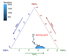
(a) AGS: $\bm{\pi}^{(2000)}_{2}=(.347,.015,.636)$

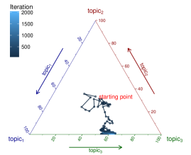
(b) MGS: $\bm{\pi}^{(2000)}_{2}=(.379,.005,.615)$

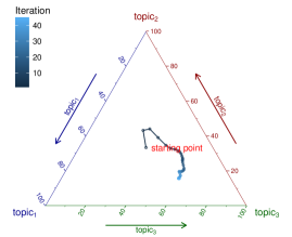
(c) VEM: $\bm{\pi}^{(45)}_{2}=(.258,.155,.585)$

Figure 3: Plots of values of $\bm{\pi}_{2}$ via algorithms AGS, MGS, and VEM. With approximately $23$ iterations the AGS chain reached the optimal region, i.e., $.07$ from the true value $\bm{\pi}^{\text{true}}_{2}=(.584,.386,.030)$, but the MGS chain took $139$ iterations to reach there. Algorithm VEM never reached the optimal regions: at convergence, VEM hit points that are $0.18$ far from $\bm{\pi}^{\text{true}}_{2}$.

[b] Method $\hat{\bm{\pi}}_{1}$^$\dagger$ $\hat{\bm{\pi}}_{2}$^$\dagger$ Iterations AGS $(\epsilon,.996,.003)$ $(.347,.015,.636)$ $2{,}000$ MGS $(.001,.997,\epsilon)$ $(.379,.005,.615)$ $2{,}000$ VEM $(.057,.935,.006)$ $(.258,.155,.585)$ $45$

Table 1: Estimated values of $\bm{\pi}$ via algorithms AGS, MGS, and VEM

• $\bm{\pi}^{\text{true}}_{1}=(.002,\epsilon,.997)$, $\bm{\pi}^{\text{true}}_{2}=(.584,.386,.030)$

3.3 Selecting Hyperparameters in cLDA

The hyperparameters $h=(\alpha,\gamma,\eta)$ in cLDA can affect the prior and posterior distributions of parameters $\psi$ and should be selected carefully. A natural solution to select them is via maximum likelihood: for example, we let $m_{{\bm{w}}}(h)$ denote the marginal likelihood of the data as a function of $h$, and use $\hat{h}=\operatorname*{arg\,max}_{h}m_{{\bm{w}}}(h)$. However, for models such as LDA and cLDA, the function $m_{{\bm{w}}}(h)$ is analytically intractable (Section 3). Works in the literature (Blei et al., 2003; Wallach, 2006) suggest an approximate EM algorithm to estimate $\operatorname*{arg\,max}_{h}m(h)$ for LDA, which can be described as follows. We consider ${\bm{w}}$ “observed data,” and $\bm{\psi}$ “missing data.” We have the “complete data likelihood” $p_{h}(\bm{\psi},{\bm{w}})$ available, then the EM algorithm (Dempster et al., 1977) is a natural candidate to estimate $\operatorname*{arg\,max}_{h}m(h)$, since $m(h)$ is the “incomplete data likelihood.” However, the E-step in EM involves calculating an expectation with respect to the intractable posterior $p_{h,{\bm{w}}}$ of the model. One solution is to approximate this expectation via variational inference (e.g. Variational-EM (Blei et al., 2003)) or Markov chain Monte Carlo (e.g. Gibbs-EM (Wallach, 2006)). We follow the latter approach for cLDA, which includes:

1. Initialize $h_{0}$ and $\bm{\psi}_{0}$

2. Until convergence

   1. Sample $\bm{\psi}_{t}^{(1)},\ldots,\bm{\psi}_{t}^{(S)}$ from $p_{h_{t},{\bm{w}}}(\bm{\psi})$ via chain AGS or MGS

   2. $h_{(t+1)}=\operatorname*{arg\,max}_{h}\sum_{s=1}^{S}\log p_{h_{t}}(\bm{\psi}_{t}^{(s)},{\bm{w}})$

One solution to M-step is via the fixed point iteration (Minka, 2000a). We derive the expressions for maximizing hyperparameter $\gamma$ and $\eta$ as follows (see Section D):

$$\eta_{(t+1)}=\frac{\eta_{t}}{V}\frac{\sum_{s,k,v}\Big{[}\Psi(m^{(s)}_{kv}+\eta_{t})-\Psi(\eta_{t})\Big{]}}{\sum_{s,k}\Big{[}\Psi(m^{(s)}_{k}+V\eta_{t})-\Psi(V\eta_{t})\Big{]}}$$ (19)

$$\gamma_{(t+1)}=\gamma_{t}\frac{\sum_{s,j,d,k}\pi^{(s)}_{jk}\Big{[}\Psi(n^{(s)}_{jdk}+\gamma_{t}\pi^{(s)}_{jk})-\Psi(\gamma_{t}\pi^{(s)}_{jk})\Big{]}}{\sum_{s,j,d}\Big{[}\Psi(n^{(s)}_{jd}+\gamma_{t})-\Psi(\gamma_{t})\Big{]}}$$ (20)

where $\sum_{x,y,\ldots}$ represents $\sum_{x=1}^{X}\sum_{y=1}^{Y}\ldots$. To illustrate the performance of the proposed method, Figure 4 shows $20$ independent Gibbs-EM estimates of cLDA hyperparameters $(\eta,\gamma)$ with default $\alpha=1$. We used a synthetic corpus with number of collections $J=2$, number of topics $K=3$, vocabulary size $V=40$, collection size = $100$, and document size = $200$ and the “true” hyperparameters $\alpha_{\text{true}}=1,\gamma_{\text{true}}=.8,\eta_{\text{true}}=.5$. We initialized the algorithm with $(\eta_{0},\gamma_{0})=(1,1)$. We notice that Gibb-EM recovered the true hyperparameters $\eta$ and $\gamma$ with a margin of error in all cases.

One approach to deal with hyperparameter $\alpha$ is to put a Gamma prior on $\alpha$ and include a posterior sampling scheme for $\alpha$. But, our sensitivity analyses on $\alpha$ shows no significant impact for $\alpha$ on the predictive power of cLDA, once we select $\eta$ and $\gamma$. We thus use a default value for $\alpha$ in our experiments.

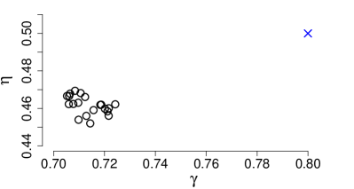
Figure 4: Independent Gibbs-EM estimates ($\circ$) of hyperparameters $(\eta,\gamma)$ in cLDA with constant hyperparmeter $\alpha=1$, for a synthetic corpora with hyperparameters $\alpha_{\text{true}}=1,\gamma_{\text{true}}=.8,\eta_{\text{true}}=.5$ ($\times$).

4 Experimental Analysis

This section compares the performance of the proposed cLDA model with alternatives, LDA and HDP, on real-world corpora (Section 4.1). We explore two performance metrics: (a) the quality of the inferred model, which we measure by the predictive power of the model (e.g. via perplexity) and external topic evaluation scores (e.g. topic coherence) (Section 4.2), and (b) the applicability of cLDA model to real-world corpora (Section 4.3). We also briefly discuss guidelines for selecting the number of topics $K$ in cLDA (Section 4.2).

4.1 Datasets

We use three document corpora based on: (i) the NIPS $00$-$18$ dataset (Globerson et al., 2007), (ii) customer reviews from Yelp, and (iii) the $20$Newsgroups dataset. Standard corpus preprocessing involve tokenizing text and discarding standard stop-words, numbers, dates, and infrequent words from the corpus. The NIPS $00$-$18$ dataset is a popular dataset used in the topic modeling community. It consists of papers published in proceedings $0$ to $18$ of the Neural Information Processing Systems (NIPS) conference (i.e. years from $1988$ to $2005$). Along with standard preprocessing, we discarded words with length less than two or with length two and not in (“ml”, “ai”, “kl”, “bp”, “em”, “ir”, “eb”) from the corpus. Finally, this corpus consists of $2{,}741$ articles and $9{,}156$ unique words. A question of interest is to see how various research topics evolve over the years $1988$-$2005$ of NIPS proceedings. Typically, new topics do not emerge in consecutive years. So, we partition the NIPS $00$-$18$ corpus into four collections based on time periods $1988$-$1992$, $1993$-$1997$, $1998$-$2002$, and $2003$-$2005$ in our analyses.

Yelp is a crowd-sourced platform for user reviews and recommendations of restaurants, shopping, nightlife, entertainment, etc. In this paper, we used a collection of restaurant reviews from Yelp. Each text review (i.e. a document) in the collection is associated with a customer rating on the scale $1$ to $5$, where $5$ being the best and $1$ being the worst. We discarded reviews with less than $50$ words. After standard preprocessing, this corpus consists of $24{,}310$ restaurant reviews and $9{,}517$ unique words.

The $20$Newsgroups dataset consists of approximately $20{,}000$ news articles that are distributed across $20$ different newsgroups. According to the subject matter of articles, these $20$ newsgroups are further partitioned into six groups. We took a subset of this dataset with the subject groups computers, recreation, science, and politics. After standard preprocessing, this corpus consists of $10{,}764$ articles and $9{,}208$ unique words. We consider the subject group of a document as its collection label to fit cLDA models. We denote this corpus by $16$Newsgroups.

4.2 Model Evaluation and Model Selection

4.2.1 Comparisons with Models in the Prior Work

(Wallach et al., 2009a, Section 3) proposed non-uniform base measures instead of the typical uniform base measures used in the Dirichlet priors over document-level topic distributions $\bm{\theta}_{d}$’s in LDA. The purpose was to get a better asymmetric Dirichlet prior for LDA, which is generally used for corpora with a flat organization hierarchy for documents. We can consider one such model as a particular case of the cLDA model proposed here: their model is closely related to a cLDA model with a single collection. To illustrate, we perform a comparative study of perplexity scores of cLDA with single and multi-collection in our experiments.

Very briefly, HDP can be described as follows. Suppose we have $D$ populations, and that for population $d,\,d=1,\ldots,D$, there are observations $w_{di}\stackrel{{\scriptstyle\text{ind}}}{{\sim}}F_{z_{di},\sigma_{di}},\,i=1,\ldots,n_{d}$. Here, $F_{z_{di},\sigma_{di}}$ is a distribution depending on some latent variable $z_{di}$ and possibly also on some other known parameter $\sigma_{di}$ particular to individual $di$. We assume that $z_{di}\stackrel{{\scriptstyle\text{iid}}}{{\sim}}G_{d},\,i=1,\ldots,n_{d}$, and that for $d=1,\ldots,D$, $G_{d}\stackrel{{\scriptstyle\text{iid}}}{{\sim}}{\cal D}_{G_{0},\alpha}$, the Dirichlet process (DP) with base probability measure $G_{0}$ and precision parameter $\alpha>0$ (Ferguson, 1973, 1974). In applications such as topic modeling, it is desirable to model the distributions of the $w_{di}$’s as mixtures, and to have mixture components shared among the distributions of the $w_{di}$’s in different populations. We can obtain this by taking $G_{0}$ itself to have a Dirichlet process prior, $G_{0}\sim{\cal D}_{{\cal K},\gamma}$, where ${\cal K}$ is a probability distribution and $\gamma>0$. In the topic modeling setting, for word $w_{di}$ of document $d$, we imagine that there exists a topic $z_{di}$—a distribution on ${\cal V}$, from which the word is drawn. Typically, the distribution ${\cal K}$ is a member of a known parametric family such as Dirichlet with parameter $\omega$. The hierarchical model described here is a two-level DP (Teh et al., 2006), which is (conceptually) similar to a one-collection cLDA model. We thus compare the results of one-collection cLDA and LDA with the results of two-level DP. We use the popular Chinese Restaurant Franchise (Teh et al., 2006, CRF) sampling scheme for inference.

4.2.2 Criteria for Evaluation

We use the perplexity computation scheme that is specified as in Patterson and Teh (2013); Wallach et al. (2009c). We first divide documents in the corpus into a training set and a held-out set. Second, we partition words in every document ${\bm{w}}_{jd}$ in the held-out set to two sets of words, ${\bm{w}}_{jd}^{\text{train}}$ and ${\bm{w}}_{jd}^{\text{test}}$. We also use ${\bm{w}}_{jd}^{\text{train}}$ to denote words in a training document $jd$. We define the vector ${\bm{w}}^{\text{train}}$ for the training corpus combining ${\bm{w}}_{jd}^{\text{train}}$, $j=1,\ldots,J$, $d=1,\ldots,D_{j}$. Similarly, we define the vector ${\bm{w}}^{\text{test}}$. We compute the per-word perplexity for the held-out words ${\bm{w}}^{\text{test}}$ (uses the fact that $z_{jdi},\,i=1,\ldots,n_{jd}$ are conditionally independent given $\bm{\theta}_{jd}$) as

$${\cal S}({\bm{w}}^{\text{test}}\,|\,{\bm{w}}^{\text{train}})=\exp\frac{-\sum_{w_{jdi}\in{\bm{w}}^{\text{test}}}\log p(w_{jdi}\,|\,{\bm{w}}^{\text{train}})}{|{\bm{w}}^{\text{test}}|}$$ (21)

where $|{\bm{w}}^{\text{test}}|$ is the length of vector ${\bm{w}}^{\text{test}}$. Exact computation of this score is intractable. However, we can estimate this score via MCMC or variational methods for both cLDA and LDA models (see Section G).

Mimno et al. (2011) suggested some generic evaluation scores based on human coherence judgments of estimated topics via topic models such as LDA. One such score is the topic size, i.e., the number of words assigned to a topic in the corpus. One can estimate it by samples from the posterior of the topic latent variable ${\bm{z}}$, given observed words ${\bm{w}}$ (e.g. via Markov chains: collapsed Gibbs sampling (CGS) for LDA (Griffiths and Steyvers, 2004), AGS, and CRF).

Another option is the topic coherence score (Mimno et al., 2011), which is computed based on the most probable words in an estimated topic for a corpus. We find the $m$ most probable words $v_{1}^{(k)},v_{2}^{(k)},\ldots,v_{m}^{(k)}$ for topic $k$ by sorting the vocabulary words in topic $k$ in the descending order of topic specific probabilities (i.e. $\beta_{kt},t=1,\ldots,V$, estimated via Markov chains such as CGS, AGS, and CRF) and picking the top $m$ words. Let $\text{df}(v_{t})$ be the document frequency of term $v_{t}$, i.e., the number of documents in the corpus which have the term $v_{t}$. Let $\text{df}(v_{i},v_{j})$ be the co-document frequency of the terms $v_{i}$ and $v_{j}$, i.e., the number of documents in the corpus which have both of the terms $v_{i}$ and $v_{j}$. We then define coherence score (Mimno et al., 2011), for topic $k=1,2,\ldots,K$, as

$$\text{topic-coherence}_{k}=\sum_{i=2}^{m}\sum_{j=1}^{i}\log\frac{\text{df}(v^{(k)}_{i},v^{(k)}_{j})+1}{\text{df}(v^{(k)}_{j})}$$ (22)

The intuition behind this score is that group of words belonging to a topic possibly co-occur with in a document.

4.2.3 Comparing Performance of cLDA and LDA Models

We first look at the criterion perplexity scores for both LDA and cLDA models with various values of the number of topics keeping each model hyperparameter fixed (and default). We ran the Markov chains AGS and CGS for $1000$ iterations. Figure 5 gives (average) per-word perplexities for the held-out (test) words using algorithms CGS and AGS (with single collection, i.e., $J=1$ and multi-collection, $J>1$) for corpora NIPS $00$-$18$, $16$Newsgroups, and yelp. From the plots, we see that cLDA outperforms LDA well in terms of predictive power, except for corpus NIPS $00$-$18$, for which cLDA has a slight edge over LDA. We believe the marginal performance for corpus NIPS $00$-$18$ is partly due to the nature of partitions defined in the corpus; collections in this corpus share many common topics, compared to corpus $16$Newsgroups. It also suggests that the gain in using cLDA is larger when we model corpora with separable collections.

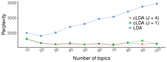
(a) $16$Newsgroups

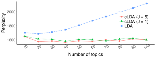
(b) Yelp

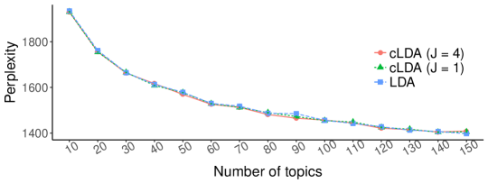
(c) NIPS $00$-$18$

Figure 5: Estimated (average) per-word perplexities for models LDA and cLDA with single collection ($J=1$), multi-collection ($J>1$) and various configurations of the number of topics $K$ using corpora $16$Newsgroups, Yelp, and NIPS $00$-$18$.

In terms of perplexity, we see a small improvement for cLDA models with multi-collection over single collection. But, the advantage of cLDA over LDA is clear, even with a single collection. Also, note that cLDA has a better selection of priors as well as the ability to incorporate document hierarchy in a corpus into the modeling framework.

Selecting $K$ and Hyperparameters $\alpha,\gamma,\eta$: Figure 5 also gives some insights on the number of topics $K$ should be used for each corpus. Perplexities of cLDA models go down quickly with increase in the number of topics in the beginning of the curves, and then the rate of decrease go steady after reasonable number of topics (e.g. $K=90$ corpus NIPS $00$-$18$). LDA, on the other hand, has a “U” curve with increase in perplexity after $K=30$ or $K=40$, for corpora $16$Newsgroups and Yelp. However, for corpus NIPS $00$-$18$, LDA shows a behavior similar to cLDA. We thus use $K=90$ for corpus NIPS $00$-$18$, $K=30$ for corpus $16$Newsgroups, and $K=40$ for corpus Yelp, in our comparative analyses in this section and case studies.

To estimate hyperparameters $\eta$ and $\gamma$ in cLDA, we use the Gibbs-EM algorithm (Section 3.3) for all three corpora with the selected $K$ and constant $\alpha=1$. Estimated $(\hat{\eta},\hat{\gamma})$’s for cLDA models at convergence for corpora $16$Newsgroups, NIPS $00$-$18$, and Yelp are $(.05,2.07)$, $(.026,6.72)$, and $(.034,3.44)$, respectively. Similarly, one can estimate hyperparameters $\alpha$ and $\eta$ in LDA based on a similar Gibbs-EM algorithm (see (19) and Wallach (2006)). Estimated $(\hat{\eta},\hat{\alpha})$’s for LDA models at convergence for corpora $16$Newsgroups, NIPS $00$-$18$, and Yelp are $(.053,.048)$, $(.027,.06)$, and $(.029,.12)$, respectively. Note that estimates $\hat{\eta}$’s for LDA and cLDA are quite similar for all three corpora.

We now evaluate distributions of topics learned by cLDA and LDA models for corpora $16$Newsgroups, NIPS $00$-$18$, and Yelp with chosen $K$ and hyperparameters $h$, quantitatively. Figure 6 shows boxplots of estimated topic sizes and coherences for models LDA and cLDA for all three corpora. Note that LDA models have uniform topic sizes compared to cLDA models. Coherence scores of cLDA topics are better than LDA topics except for corpus $16$Newsgroups, which we think, is partially due to having relatively easily separable topics compared to the other two complex corpora.

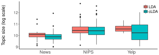
(a) Topic size

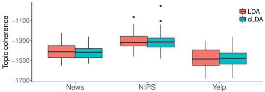
(b) Topic coherence

Figure 6: Estimated topic sizes and coherences for models LDA and cLDA for corpus $16$Newgroups, NIPS $00$-$18$, and Yelp.

Execution time: In our experience, both AGS (with a reasonable number of collections) and CGS chains have comparable computational cost for all three corpora (details in Table 2). On average, the combined execution-time of multiple CGS runs for a corpus that is partitioned on collection labels was fairly equivalent to the execution-time of a single CGS run on the whole corpus. We implemented all these algorithms single-threaded on the R-C++ (using the efficient Rcpp and RcppArmadillo libraries) programming environment.

[b] Corpus Number of Topics CGS AGS MGS^a VEM^b $16$Newsgroups $64$ $0.6101$ $0.6879$ $1.8616$ $52.3518$ NIPS $00$-$18$ $90$ $3.9568$ $4.2588$ $12.5580$ $320.9931$ Yelp $60$ $1.2997$ $1.4743$ $3.9524$ $164.0285$

Table 2: Average per iteration execution time (in seconds) for various topic modeling algorithms.

• MGS chains took approximately twice or more the execution time of CGS chains for all three corpora.

• We can see that per iteration running cost for VEM is relatively high for these corpora. We believe that this due to the single-threaded vanilla implementation for VEM; it may be improved by an efficient parallel implementation, which we leave to future research.

4.2.4 Comparing Performance of cLDA with LDA and HDP

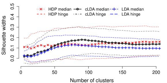
Figure 16: Boxplot statistics (median, lower hinge, and upper hinge) of silhouette widths computed on documents’ hclust clusters with various values of the number of clusters, for corpus NIPS $00$-$18$. Algorithm hclust was applied on documents’ topic distributions estimated via cLDA, LDA, and HDP sampling algorithms. Silhouette widths of clusters based on HDP are relatively constant with different values of the number of clusters. HDP estimated large set of minute topics ($K=204$), which may have helped clustering documents. cLDA performs better than LDA, and is comparable with HDP or better than HDP with the right number of hclust clusters (e.g. from $50$ to $150$). See discussion in Section 4.2.

We now compare the performance of one-collection cLDA and LDA with two-level DP using corpus NIPS $00$-$18$. We ran all the three chains AGS, CGS, and CRF for $1{,}000$ iterations and used the last sample from each chain for our analysis. We used fixed $K=90$ for both algorithms AGS and CGS, but algorithm CRF inferred $204$ topics from the corpus. We first evaluate the quality of topics learned for each method, by applying the hclust algorithm on topic distributions. hclust first computes a topic-to-topic similarity matrix based on the manhattan distance. Then, it builds a hierarchical tree in a bottom-up approach. We noticed that the hierarchies formed by cLDA and LDA are comparable. By looking closely at topic word distributions, we notice that cLDA produces better topics, exploiting the asymmetric hierarchical Dirichlet prior on document $\bm{\theta}_{d}$’s that which is absent in LDA. (details, Section H). HDP, on the other hand, found too many redundant topics, as shown in Figure 8. To evaluate clusters induced by hclust quantitatively, we look at silhouette widths computed on topics’ hclust clusters. We favor methods with high silhouette widths. Figure 7 gives boxplot statistics (i.e. median, lower hinge, and upper hinge) of silhouette widths computed on topics’ hclust clusters with various values of the number of clusters (a user specified value in hclust). Overall, cLDA topics outperform HDP topics, and cLDA topics are comparable or better than LDA topics. Our analysis on clustering on learned document topic proportions, i.e., $\bm{\theta}_{d}$s, also show similar results (Figure 16)

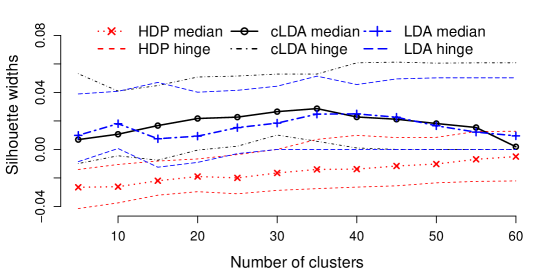
Figure 7: Boxplot statistics (median, lower hinge, and upper hinge) of silhouette widths computed on topics’ hclust clusters (i.e. hierarchical clustering of topic distributions) with various values of the number of clusters, for corpus NIPS $00$-$18$

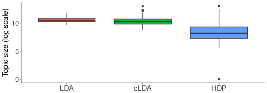
Figure 8: Estimated topic sizes for models LDA, cLDA, and HDP for corpus NIPS $00$-$18$.

4.3 Usability Study

In text mining, one can use trained cLDA models for tasks such as classifying text documents and summarizing document collections and corpora. cLDA also gives excellent options to visualize and browse documents. To illustrate some of these, we provide a usability study for the proposed cLDA model next. We are interested in two aspects of a learned cLDA model: (a) interpretability of the learned topics and topic structures, and (b) visualizing corpora in terms of learned topics.

cLDA infers collection-level and document-level topic distributions based on a common set of corpus-level topics. So it is natural to check whether cLDA’s topics are as interpretable as LDA’s topics. We present three examples of LDA and cLDA topics t$8$, t$57$, and t$85$ in Figure 9 to furnish a qualitative comparison of these models, for corpus NIPS $00$-$18$. For each topic $k$, we show $20$ most probable words based on the non-decreasing order of the $\beta_{kv}$ values over words $v$’s (denoted by bars in each plot). Note that we did any necessary alignments for the set of topics from each of these models to ease comparison. We labeled topics based on their most probable words. (We do these post processing steps for this section and all the following.) Note that cLDA topics are meaningful, easily interpretable, and comparable with LDA topics.

(a) cLDA: t$8$ (ANN)

(b) cLDA: t$57$ (MCMC)

(c) cLDA: t$85$ (Bayesian models)

(d) LDA: t$8$ (ANN)

(e) LDA: t$57$ (MCMC)

(f) LDA: t$85$ (Bayesian models)

Figure 9: $20$ most probable words for topics from $90$-topic cLDA (top row) and LDA (bottom row) models trained on corpus NIPS $00$-$18$. Bars represent the corresponding (estimated) probabilities of words given a topic.

A typical question of interest in topic modeling is to identify topics that evolve over time. cLDA provides a way to model time evolving corpus. On the other hand, LDA has some limitations due to several issues such as the required alignment of topics and information loss of segmentation, as mentioned in Section 1. To illustrate some of these issues involved, we study corpus NIPS $00$-$18$—consists of four collections based on document timestamps—using both cLDA and LDA models. Once we fit a cLDA model (e.g. via AGS chain) for the corpus, we can use each estimated collection-level topic distribution for a time period as its natural topic allocation. Recall that LDA does not have collection-level topic mixtures by the model construction. However, one can estimate them via each collection’s word topic vector ${\bm{z}}_{j}$ (e.g. sampled from the CGS chain).

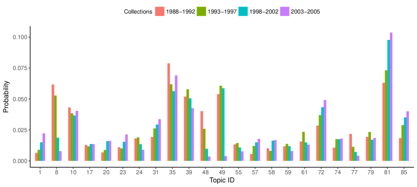
Figure 18: Estimates of topic distributions for four collections (defined on timespans $1988$-$1992$, $1993$-$1997$, $1998$-$2002$, and $2003$-$2005$) of the NIPS $00$-$18$ corpus via the cLDA AGS algorithm.

Figure 10 shows estimates of four collection-level topic distributions $\bm{\pi}_{1},\bm{\pi}_{2},\bm{\pi}_{3}$, and $\bm{\pi}_{4}$ for corpus NIPS $00$-$18$ based on three different topic modeling approaches, which we will describe below. In Figure 10a, we applied the cLDA AGS algorithm on the whole corpus with four collections, i.e., $J$ = 4 (denoted by M$1$). Each barplot represents the value of a topic element in the last sample $\bm{\pi}^{(1000)}$ from the AGS chain. (We show values for a few selected topics here; see an extended list of topics in the Appendix, Figure 18.) Figure 10b is based on the LDA CGS algorithm on the whole corpus (denoted by M$2$). To estimate collection $j$’s topic mixture, we used the last sample ${\bm{z}}_{j}^{(1000)}$ from the CGS chain. In Figure 10c, we considered each collection in the corpus as a separate corpus. We then ran the LDA CGS algorithm on each sub-corpus (denoted by M$3$) one by one. We used the last sample ${\bm{z}}_{j}^{(1000)}$ from collection $j$’s CGS chain to estimate its topic mixture.

One can infer interesting patterns from the estimates of collection-level topic mixtures via method M$1$, as shown in Figure 10a. Several research topics got increased and decreased interest, and some topics were relatively constant in popularity over the time span $1988$-$2005$ of NIPS. As we would have expected, topic t$57$, a topic on MCMC and inference, and topic t$85$, a topic on generative models got increased popularity over the time span, which is interesting to watch. One topic that lost popularity is t$8$, which is about neural networks and related topics. (Additional details are given in Section H.) We can also see that the estimates via method M$1$ are superior to the estimates based on other two methods M$2$ and M$3$. Note that for method M$3$, one must solve the non-trivial topic alignment problem for each LDA model learned for every sub-corpus. Additionally, we notice that method M$2$ gives better estimates than method M$3$. We believe this is due to the lack of information sharing among the partitions in method M$3$ that might have affected the quality of the learned LDA models. On the other hand, cLDA considers the corpus as a whole to incorporate the organization hierarchy of documents into the model, eliminating the issues discussed.

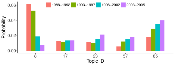
(a) M$1$: AGS run on the corpus with four collections

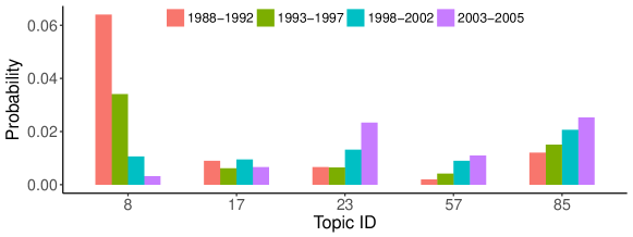
(b) M$2$: Single CGS run on the whole corpus

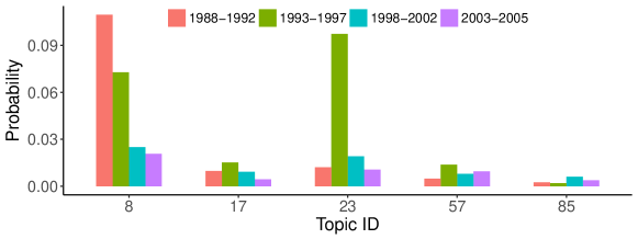
(c) M$3$: Single CGS run on each of the four partitions of the corpus

Figure 10: Estimates of topic distributions (of five randomly selected topics) for four timespans $1988$-$1992$, $1993$-$1997$, $1998$-$2002$, and $2003$-$2005$ of the NIPS conference proceedings via three topic modeling approaches. Clearly, cLDA identifies interpretable topic patterns compared to other two LDA approaches. See discussion in the text.

Modeling customer behaviors is the core interest in operations management community and market research. Analyzing patterns of topics that pervade through customer reviews can give interesting insights about customer needs. We wish to study topic patterns for different customer ratings, and we thus use corpus Yelp. A natural choice is to partition the corpus into collections based on customer review ratings on the scale $1$-$5$, and fit a cLDA model. Note that the two other corpora used in this paper have collections that occurred more naturally; but, for this corpus, we follow this partitioning scheme just for experimentation. Figure 11a shows estimated collection-level topic distributions of a $40$-topic cLDA model trained on corpus Yelp via AGS chain. Specifically, each barplot represents the value of a topic element for a collection from the last sample $\bm{\pi}^{(1000)}$ of the AGS chain. We can see a gradual increase of probabilities for some topics (e.g. t$3$, t$11$, t$26$) and gradual decrease of probabilities for some topics (e.g. t$7$, t$14$, t$18$), for rating from $1$ to $5$. We noticed that the topics with gradual increase in probabilities correspond to positive reviews, and the topics with gradual decrease in probabilities correspond to negative reviews.

Table 3 gives additional details of these topics and their manually assigned sentiment. In our experience, people do not give detail reviews about the place, ambiance, food, or customer service, if they really like them (e.g. reviews with rating $5$). If they partially like a place (e.g. reviews with rating $3$ and $4$), they provide comments with all the details. Additionally, topics that show little or relatively small variability for different ratings are general topics about food styles. For completeness, we include the collection-level topic distributions estimated via a single CGS chain (i.e. via method M$2$) for the same Yelp corpus with $K=40$. Note that LDA is inferior in giving any interpretable analyses from the results, as shown in Figure 11b.

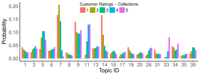
(a) M$1$: AGS run on the corpus with five collections

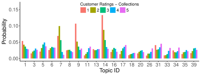
(b) M$2$: Single CGS run on the whole corpus

Figure 11: Estimates of topic proportions for five customer ratings $1$, $2$, $3$, $4$, and $5$ via algorithms AGS and CGS using the Yelp corpus. Table 3 gives additional details about the listed topics. Clearly, cLDA provides meaningful and interpretable patterns of topics in the corpus for different customer ratings, compared to its non-hierarchical precursor, LDA. In both of these models, topics are aligned to ease comparison, based on most probable words given a topic. See description in the text.

[b] Topic ID^a Sentiment Short Description 3 positive food 11 positive food, place 26 positive food, ambiance, group dining 33 positive food, atmosphere 5 moderately positive food, service 6 moderately positive food 13 moderately positive food, waiting time 35 moderately positive food, sandwich, salad 39 moderately positive place, ambiance 8 neutral Mexican food 9 neutral place, food 16 neutral bar, food, atmosphere 20 neutral location, parking 34 neutral location, ambiance 1 moderately negative ambiance, night-life 7 moderately negative food, service 31 moderately negative food, meal quantity 14 negative food, service 18 negative place, food

Table 3: A subset of topics from a $40$-topic cLDA model for corpus Yelp

• The topics are ordered in the non-decreasing order of the positive sentiment or polarity of the most probable words given a topic.

A key feature of the cLDA model, compared to its non-hierarchical alternative, LDA, is that it provides collection level topics, which summarize themes or topics of individual collections in a corpus. We perform a study on the applicability of this feature using corpus $16$newsgroups. Recall that corpus $16$newsgroups is partitioned based on four subject groups. It is natural to check whether each collection’s topic distribution exhibits proper weights to the topics that are related to the subject matter of the collection. Figure 12 shows estimated collection-level topic distributions, i.e., $\bm{\pi}_{j},\,j=1,\ldots,4$, from a learned $30$-topic cLDA model via the AGS algorithm. (We found that topic $10$, which is dominant in all collections, is a potential collection of stop-words in the corpus. Figure 19 provides examples of topics for reference.) The results show that cLDA enables us to summarize topics of individual collections and perform a meaningful comparison of topics among collections, an aspect that is not well exploited in a flat modeling framework such as LDA. We also notice sparse allocations for topics in each collection and no major sharing of topics among collections in Figure 12: this conveys the fact that corpus $16$newsgroups may be surely separable via the subject matter of newsgroups.

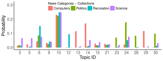
Figure 12: Estimates of topic distributions for collections Computers, Politics, Recreation, and Science in corpus $16$newsgroups.

5 Summary

In this paper, we developed a topic model, compound latent Dirichlet allocation (cLDA), that can incorporate several characteristics of a corpus including the organization hierarchy of documents. One can employ cLDA model to (a) explore research topics across multiple/consecutive proceedings or workshops of a conference, (b) discover cultural differences in blogs and forums from different countries, or (c) compare nuanced review summarization on various customer ratings (for customer relations management). We proposed posterior inference methods for cLDA (e.g. AGS, MGS, VEM), which can be used for analyzing collections of documents and we recommend algorithm AGS. We also discussed guidelines for selecting $K$ and hyperparameters in cLDA, which perform well empirically. Additionally, we have seen that proposed parametric hierarchy in cLDA adds only a little computational burden compared to the non-hierarchical alternative, LDA. cLDA model makes several natural assumptions about the data generating framework, which we believe helped us getting a much simpler inference scheme, compared to nonparametric alternatives such as Hierarchical Dirichlet Process (Teh et al., 2006). We have also provided an empirical comparison of cLDA with two-level DP.

Lastly, we studied the applicability and performance of cLDA model in both synthetic and real-world corpora. cLDA is quite useful for analyzing topic distributions of collections in a corpus, and it can better understand the underlying thematic structure of the corpus. cLDA provides relevant insights about topics that evolve over time, as noted in the experiments on NIPS conference proceedings. This model also presents some ideas to employ metadata such as customer ratings for “soft” segmentation while analyzing the thematic structure of customer reviews. Although such partitions do not emerge naturally, together with cLDA, they may provide diverse perspectives of customer behaviors.

We also wish to study the applicability of this model for a corpus where documents exhibit multiple collection memberships. For example, a corpus built from the Wikipedia articles, where an article can be assigned to one or more Wikipedia categories.

Appendix A Expressions for the Prior, Likelihood, and Posterior

This section derives expressions of the prior $p_{h}(\bm{\psi})$, likelihood $\ell_{{\bm{w}}}(\bm{\psi})$, and the posterior $p_{h,{\bm{w}}}(\bm{\psi})$. From the hierarchical model (1)–(5) given in Section 2, we can write the prior $p_{h}(\bm{\psi})$ as

$$p_{h}({\bm{z}}\,|\,\bm{\theta},\bm{\pi},\bm{\beta})p_{h}(\bm{\theta}\,|\,\bm{\pi})p_{h}(\bm{\pi})p_{h}(\bm{\beta}),$$

where the individual density functions are given by (1)–(4) of the model. Let $n_{jdk}=\sum_{i=1}^{n_{jd}}z_{jdik}$, i.e. $n_{jdk}$ is the number of words in document $d$ in collection $j$ that are assigned to topic $k$, and let $n_{j.k}=\sum_{d=1}^{D_{j}}\sum_{i=1}^{n_{jd}}z_{jdik}$, i.e. $n_{j.k}$ is the number of words in all documents in collection $j$ that are assigned to topic $k$. Using the Dirichlet and multinomial distributions specified in (1)–(4), we obtain

$$p_{h}(\bm{\psi}) = \prod_{j=1}^{J}\left(\frac{\Gamma\bigl{(}K\alpha\bigr{)}}{\Gamma(\alpha)^{K}}\prod_{k=1}^{K}\pi_{jk}^{\alpha-1}\right)\Biggl{[}\prod_{j=1}^{J}\prod_{d=1}^{D_{j}}\prod_{k=1}^{K}\theta_{jdk}^{n_{jdk}}\Biggr{]}$$ (23)

$$\Biggl{[}\prod_{j=1}^{J}\prod_{d=1}^{D_{j}}\Biggl{(}\frac{\Gamma\bigl{(}\gamma\bigr{)}}{\prod_{k=1}^{K}{\Gamma(\gamma\pi_{jk})}}\prod_{k=1}^{K}\theta_{jdk}^{\gamma\pi_{jk}-1}\Biggr{)}\Biggr{]}$$

$$\Biggl{[}\prod_{k=1}^{K}\biggl{(}\frac{\Gamma(V\eta)}{\Gamma(\eta)^{V}}\prod_{v=1}^{V}\beta^{\eta-1}_{kv}\biggr{)}\Biggr{]}.$$

For $j=1,\ldots,J$, $d=1,\ldots,D_{j}$ and $k=1,\ldots,K$, let $S_{jdk}=\{i:1\leq i\leq n_{jd}\text{ and }z_{jdik}=1\}$, which is the set of indices of all words in document $d$ in collection $j$ whose latent topic variable is $k$. With this notation, Equation (4) induces the likelihood function $\ell_{{\bm{w}}}(\bm{\psi}):=p({\bm{w}}\,|\,{\bm{z}},\bm{\theta},\bm{\pi},\bm{\beta})$

$$\begin{split}p({\bm{w}}\,|\,{\bm{z}},\bm{\theta},\bm{\pi},\bm{\beta})&=\prod_{j=1}^{J}\prod_{d=1}^{D_{j}}\prod_{i=1}^{n_{jd}}\prod_{k:z_{jdik}=1}\prod_{v=1}^{V}\beta_{kv}^{w_{jdiv}}\\ &=\prod_{j=1}^{J}\prod_{d=1}^{D_{j}}\prod_{k=1}^{K}\prod_{v=1}^{V}\prod_{i\in S_{jdk}}\beta_{kv}^{w_{jdiv}}\\ &=\prod_{j=1}^{J}\prod_{d=1}^{D_{j}}\prod_{k=1}^{K}\prod_{v=1}^{V}\beta_{kv}^{\sum_{i\in S_{jdk}}w_{jdiv}}\\ &=\prod_{j=1}^{J}\prod_{d=1}^{D_{j}}\prod_{k=1}^{K}\prod_{v=1}^{V}\beta_{kv}^{m_{jdkv}},\end{split}$$ (24)

where $m_{jdkv}=\sum_{i\in S_{jdk}}w_{jdiv}$ counts the number of words in document $d$ in collection $j$ for which the latent topic is $k$ and the index of the word in the vocabulary is $v$. Recalling the definition of $n_{jdk}$ given just before (23), and noting that $\sum_{i\in S_{jdk}}w_{jdiv}=\sum_{i=1}^{n_{jd}}z_{jdik}w_{jdiv}$, we see that $m_{jdkv}=\sum_{i=1}^{n_{jd}}z_{jdik}w_{jdiv}$ and $\sum_{v=1}^{V}m_{jdkv}=n_{jdk}$

Plugging the likelihood (24) and the prior (23) into the expression for the Bayes rule (6), and absorbing constants in Dirichlet normalizing constants into an overall constant of proportionality, we have the posterior density

$$\begin{split}p_{h,{\bm{w}}}(\bm{\psi})&\propto\Biggl{[}\prod_{k=1}^{K}\prod_{v=1}^{V}\beta_{kv}^{\sum_{j=1}^{J}\sum_{d=1}^{D_{j}}m_{jdkv}+\eta-1}\Biggr{]}\\ &\hskip 13.37277pt\Biggl{[}\prod_{j=1}^{J}\prod_{d=1}^{D_{j}}\frac{\prod_{k=1}^{K}\theta_{jdk}^{n_{jdk}+\gamma\pi_{jk}-1}}{\prod_{k=1}^{K}{\Gamma(\gamma\pi_{jk})}}\Biggr{]}\Biggl{[}\prod_{j=1}^{J}\prod_{k=1}^{K}\pi_{jk}^{\alpha-1}\Biggr{]}\end{split}$$

Appendix B Conditional posterior for $z_{jdi}$

This section derives a closed form expression for the conditional posterior $p_{h,{\bm{w}}}\left(z_{jdik}=1\,|\,{\bm{z}}^{(-jdi)},\bm{\pi}\right)$ for $k=1,\ldots,K$. The vector ${\bm{z}}^{(-jdi)}$ contains topic assignments of all words in the corpus except for word $w_{jdi}$. We can then write

$$\begin{split}p_{h,{\bm{w}}}\left(z_{jdik}=1\,|\,{\bm{z}}^{(-jdi)},\bm{\pi}\right)&\propto p\left(z_{jdik}=1,w_{jdiv}=1\,|\,{\bm{z}}^{(-jdi)},{\bm{w}}^{(-jdi)},\bm{\pi}\right)\\ &=\frac{p\left(z_{jdik}=1,w_{jdiv}=1,{\bm{z}}^{(-jdi)}\,|\,{\bm{w}}^{(-jdi)},\bm{\pi}\right)}{p\left({\bm{z}}^{(-jdi)}\,|\,{\bm{w}}^{(-jdi)},\bm{\pi}\right)}\\ &\propto\frac{\gamma\pi_{jk}+n^{(-jdi)}_{jdk}}{\gamma+n^{(-jdi)}_{jd.}}\,\frac{\eta+m^{(-jdi)}_{..kv}}{V\eta+m^{(-jdi)}_{..k.}}\end{split}$$ (25)

Here, we used the fact that $p\left({\bm{z}}^{(-jdi)}\,|\,{\bm{w}}^{(-jdi)},\bm{\pi}\right)\propto p_{h,{\bm{w}}}(\bm{\pi},{\bm{z}})^{(-jdi)}$ given by (9) and $\Gamma(x+1)=x\Gamma(x)$. The superscript $(-jdi)$ means that we discard the contribution of word $w_{jdi}$ in count statistics $n_{jdk}$, $n_{jd.}$, $m_{..kv}$, and $m_{..k.}$. This development is motivated by the LDA collapsed Gibbs sampling algorithm (Griffiths and Steyvers, 2004, CGS).

Appendix C Langevin Monte Carlo

The Metropolis Adjusted Langevin Algorithm  (Girolami and Calderhead, 2011, MALA), as described in Section 3.1.2, is given the following steps

1. Propose $\bm{\pi}^{(*)}$ via Langevin dynamics (17)

2. Calculate the MH acceptance ratio

   $$a(\bm{\pi}^{(t)},\bm{\pi}^{(*)})=\frac{p(\bm{\pi}^{(*)})}{p(\bm{\pi}^{(t)})}\frac{\exp\bigl{(}-\frac{1}{2\varepsilon^{2}}{\|\bm{\pi}^{(t)}-{\bm{\mu}}(\bm{\pi}^{(*)},\varepsilon)\|}^{2}\bigr{)}}{\exp\bigl{(}-\frac{1}{2\varepsilon^{2}}{\|\bm{\pi}^{(*)}-{\bm{\mu}}(\bm{\pi}^{(t)},\varepsilon)\|}^{2}\bigr{)}}$$ (26)

   and set $\bm{\pi}^{(t+1)}=\bm{\pi}^{(*)}$ with probability min$(1,a(\bm{\pi}^{(t)},\bm{\pi}^{(*)}))$, and set $\bm{\pi}^{(t+1)}=\bm{\pi}^{(t)}$ with the remaining probability.

C.1 Riemann Manifold Metropolis Adjusted Langevin Algorithm

Girolami et al. (Girolami and Calderhead, 2011, Section 5) suggests the preconditioning matrix ${{\bm{G}}}(\bm{\pi})$ as an arbitrary metric tensor on a Riemannian manifold induced by the parameter space of a statistical model. We write the stochastic differential equation for the Langevin diffusion on the Riemannian manifold as

$$\text{d}\bm{\pi}(t)=\frac{1}{2}\widetilde{\nabla}_{\bm{\pi}}{\cal L}(\bm{\pi}^{(t)})\text{d}t+\text{d}\tilde{{\bm{b}}}(t)$$ (27)

where the natural gradient is

$$\widetilde{\nabla}_{\bm{\pi}}{\cal L}(\bm{\pi}^{(t)})={\bm{G}}\{\bm{\pi}(t)\}^{-1}\nabla_{\bm{\pi}}{\cal L}(\bm{\pi}^{(t)})$$ (28)

and the Brownian motion is

$$\text{d}\tilde{{\bm{b}}}_{k}(t)={|{\bm{G}}\{\bm{\pi}(t)\}|}^{-1/2}\sum_{k^{\prime}=1}^{K}\frac{\partial}{\partial\pi_{k^{\prime}}}\Bigl{[}{\bm{G}}\{\bm{\pi}(t)\}^{-1}_{kk^{\prime}}\,{|{\bm{G}}\{\bm{\pi}(t)\}|}^{1/2}\Bigl{]}\text{d}t+{\Bigl{[}{{\bm{G}}\{\bm{\pi}(t)\}}^{-1/2}\text{d}{\bm{b}}(t)\Bigl{]}}_{k}$$ (29)

where the subscript $k$ indicates $k^{\text{th}}$ element in vector $\text{d}\tilde{{\bm{b}}}(t)$. Note that in the Euclidean space the metric tensor ${{\bm{G}}}(\bm{\pi})$ is an identity matrix, and thus (27) will be reduced to the standard Langevin SDE.

By expanding the gradients in (29) and discretizing (27) via the first-order Euler integration, we get the proposal for the Riemann Manifold Metropolis Adjusted Langevin Algorithm (MMALA):

$$\bm{\pi}^{(*)}={\bm{\mu}}(\bm{\pi}^{(t)},\varepsilon)+\varepsilon{{\bm{G}}(\bm{\pi}^{(t)})}^{-1/2}{\bm{\xi}}^{(t)},$$ (30)

where $k^{\text{th}}$ element in vector ${\bm{\mu}}(\bm{\pi}^{(t)},\varepsilon)$ is given by

$$\begin{split}{\bm{\mu}}(\bm{\pi}^{(t)},\varepsilon)_{k}&=\pi_{k}^{(t)}+\frac{\varepsilon^{2}}{2}\Bigl{\{}{{\bm{G}}(\bm{\pi}^{(t)})}^{-1}\nabla_{\bm{\pi}}{\cal L}(\bm{\pi}^{(t)})\Bigr{\}}_{k}\\ &\hskip 14.22636pt-\varepsilon^{2}\sum_{k^{\prime}=1}^{K}\Bigl{\{}{\bm{G}}(\bm{\pi}^{(t)})^{-1}\frac{\partial{\bm{G}}(\bm{\pi}^{(t)})}{\partial\pi_{k^{\prime}}}{\bm{G}}(\bm{\pi}^{(t)})^{-1}\Bigr{\}}_{kk^{\prime}}\\ &\hskip 14.22636pt+\frac{\varepsilon^{2}}{2}\sum_{k^{\prime}=1}^{K}\bigl{\{}{\bm{G}}(\bm{\pi}^{(t)})^{-1}\bigl{\}}_{kk^{\prime}}\text{tr}\Bigl{\{}{\bm{G}}(\bm{\pi}^{(t)})^{-1}\frac{\partial{\bm{G}}(\bm{\pi}^{(t)})}{\partial\pi_{k^{\prime}}}\Bigr{\}}\end{split}$$ (31)

The corresponding proposal density is given by

$$q(\bm{\pi}^{(*)}\leftarrow\bm{\pi}^{(t)})=\mathcal{N}_{K}(\bm{\pi}^{(*)}\,|\,{\bm{\mu}}(\bm{\pi}^{(t)},\varepsilon),\,\varepsilon^{2}{\bm{G}}(\bm{\pi}^{(t)})^{-1})$$ (32)

C.2 Langevin Updates on Probability Simplices: Boundary Considerations

We first re-write the unnormalized conditional density (11) on $\bm{\pi}_{j}$ as

$$\tilde{p}({\bm{\varphi}}_{j}\,|\,{\bm{z}}_{j},{\bm{w}}_{j})\propto\prod_{d=1}^{D_{j}}\prod_{k=1}^{K}\Biggl{(}\frac{\Gamma(\gamma\frac{|\varphi_{jk}|}{|\varphi_{j.}|}+n_{jdk})}{\Gamma(\gamma\frac{|\varphi_{jk}|}{|\varphi_{j.}|})}\Biggr{)}\prod_{k=1}^{K}{|\varphi_{jk}|}^{\alpha-1}e^{-|\varphi_{jk}|}$$ (33)

The MMALA update for the new parametrization is given by

$${\bm{\varphi}}_{j}^{(*)}={\bm{\mu}}({\bm{\varphi}}_{j}^{(t)},\varepsilon)+\varepsilon{{\bm{G}}({\bm{\varphi}}_{j}^{(t)})}^{-1/2}{\bm{\xi}}^{(t)}$$ (34)

where for $k=1,\ldots,K$, we have

$$\begin{split}{\bm{\mu}}({\bm{\varphi}}_{j}^{(t)},\varepsilon)_{k}&=\varphi_{jk}^{(t)}+\frac{\varepsilon^{2}}{2}\Bigl{\{}{{\bm{G}}({\bm{\varphi}}_{j}^{(t)})}^{-1}\nabla_{{\bm{\varphi}}_{j}}{\cal L}({\bm{\varphi}}_{j}^{(t)})\Bigr{\}}_{k}\\ &\hskip 14.22636pt-\varepsilon^{2}\sum_{k^{\prime}=1}^{K}\Bigl{\{}{\bm{G}}({\bm{\varphi}}_{j}^{(t)})^{-1}\frac{\partial{\bm{G}}({\bm{\varphi}}_{j}^{(t)})}{\partial\varphi_{jk^{\prime}}}{\bm{G}}({\bm{\varphi}}_{j}^{(t)})^{-1}\Bigr{\}}_{kk^{\prime}}\\ &\hskip 14.22636pt+\frac{\varepsilon^{2}}{2}\sum_{k^{\prime}=1}^{K}\bigl{\{}{\bm{G}}({\bm{\varphi}}_{j}^{(t)})^{-1}\bigl{\}}_{kk^{\prime}}\text{tr}\Bigl{\{}{\bm{G}}({\bm{\varphi}}_{j}^{(t)})^{-1}\frac{\partial{\bm{G}}({\bm{\varphi}}_{j}^{(t)})}{\partial\varphi_{jk^{\prime}}}\Bigr{\}}\end{split}$$ (35)

The proposal density of this diffusion process is given by

$$\begin{split}q({\bm{\varphi}}_{j}^{(*)}\leftarrow{\bm{\varphi}}_{j}^{(t)})&=\mathcal{N}_{K}({\bm{\varphi}}_{j}^{(*)}\,|\,{\bm{\mu}}({\bm{\varphi}}_{j}^{(t)},\varepsilon),\,\varepsilon^{2}{\bm{G}}({\bm{\varphi}}_{j}^{(t)})^{-1})\\ &\propto{|{\bm{G}}({\bm{\varphi}}_{j}^{(t)})^{-1}|}^{-1/2}\exp\Bigl{\{}-\frac{1}{2\varepsilon^{2}}{({\bm{\varphi}}_{j}^{(*)}-{\bm{\mu}}({\bm{\varphi}}_{j}^{(t)},\varepsilon))}^{\text{T}}{\bm{G}}({\bm{\varphi}}_{j}^{(t)}){({\bm{\varphi}}_{j}^{(*)}-{\bm{\mu}}({\bm{\varphi}}_{j}^{(t)},\varepsilon))}\Bigr{\}}\\ \end{split}$$ (36)

We take the metric tensor ${\bm{G}}({\bm{\varphi}}^{(t)}_{j})$ as $\operatorname{diag}(|{\bm{\varphi}}^{(t)}_{j}|)^{-1}$ (Patterson and Teh (2013) suggested this choice in a different context.), as it gives simplified expressions for

$${\bm{\mu}}({\bm{\varphi}}_{j}^{(t)},\varepsilon)_{k}=\varphi_{jk}^{(t)}+\frac{\varepsilon^{2}}{2}\,\Bigl{\{}\operatorname{diag}(|{\bm{\varphi}}_{j}^{(t)}|)\,\nabla_{{\bm{\varphi}}_{j}}{\cal L}({\bm{\varphi}}_{j}^{(t)})\Bigr{\}}_{k}+\frac{\varepsilon^{2}}{2}\,\operatorname{sign}(\varphi^{(t)}_{jk})$$ (37)

and

$$q({\bm{\varphi}}_{j}^{(*)}\leftarrow{\bm{\varphi}}_{j}^{(t)})\propto\Bigl{[}\prod_{k=1}^{K}{|\varphi_{jk}^{(t)}|}^{-1/2}\Bigr{]}\exp\Bigl{\{}-\frac{1}{2\varepsilon^{2}}{({\bm{\varphi}}_{j}^{(*)}-{\bm{\mu}}({\bm{\varphi}}_{j}^{(t)},\varepsilon))}^{\text{T}}\operatorname{diag}({|{\bm{\varphi}}_{j}^{(t)}|})^{-1}{({\bm{\varphi}}_{j}^{(*)}-{\bm{\mu}}({\bm{\varphi}}_{j}^{(t)},\varepsilon))}\Bigr{\}}$$ (38)

To derive $\nabla_{{\bm{\varphi}}_{j}}{\cal L}({\bm{\varphi}}_{j}^{(t)})$, we first write $\tilde{p}({\bm{\varphi}}_{j}\,|\,{\bm{z}}_{j},{\bm{w}}_{j})$ in a convenient logarithmic form:

$$\log\tilde{p}({\bm{\varphi}}_{j}\,|\,{\bm{z}}_{j},{\bm{w}}_{j})\propto\sum_{k=1}^{K}\Bigl{[}\Bigl{\{}(\alpha-1)\log|\varphi_{jk}|\Bigr{\}}-|\varphi_{jk}|\Bigr{]}+\sum_{d=1}^{D_{j}}\sum_{k=1}^{K}\Bigl{[}\log\Gamma(\gamma\frac{|\varphi_{jk}|}{|\varphi_{j.}|}+n_{jdk})-\log\Gamma(\gamma\frac{|\varphi_{jk}|}{|\varphi_{j.}|})\Bigr{]}$$

We then define $\nabla_{{\bm{\varphi}}_{j}}{\cal L}({\bm{\varphi}}_{j}^{(t)})$ by the partial derivatives

$$\begin{split}\frac{\partial\log\tilde{p}({\bm{\varphi}}_{j}\,|\,{\bm{z}}_{j},{\bm{w}}_{j})}{\partial\varphi_{jk^{*}}}&=\operatorname{sign}(\varphi_{jk^{*}})\Bigl{\{}\frac{\gamma}{{|\varphi_{j.}|}^{2}}\sum_{d=1}^{D_{j}}\sum_{k=1}^{K}{|\varphi_{jk}|}\Bigl{[}\varPsi(\gamma\frac{{|\varphi_{jk}|}}{{|\varphi_{j.}|}})-\varPsi(\gamma\frac{{|\varphi_{jk}|}}{{|\varphi_{j.}|}}+n_{jdk})\Bigr{]}\\ &\hskip 11.38109pt-\frac{\gamma}{{|\varphi_{j.}|}}\sum_{d=1}^{D_{j}}\Bigl{[}\varPsi(\gamma\frac{{|\varphi_{jk^{*}}|}}{{|\varphi_{j.}|}})-\varPsi(\gamma\frac{{|\varphi_{jk^{*}}|}}{{|\varphi_{j.}|}}+n_{jdk^{*}})\Bigr{]}+\Bigl{[}\frac{(\alpha-1)}{{|\varphi_{jk^{*}}|}}-1\Bigr{]}\Bigr{\}}\\ \end{split}$$ (39)

Similar to the AGS chain, in this scheme, we implement a Markov chain on $(\bm{\pi},{\bm{z}})$ via MMALA updates within Gibbs sampling (MGS), as in Algorithm 2.

Appendix D Estimating hyperparameters $\eta$ and $\gamma$

In this section, we derive expressions for the fixed point iterations of hyperparameters $\eta$ and $\gamma$ in the cLDA model. We use the following two bounds by (Minka, 2000a, Appendix B) in our development.

$$\frac{\Gamma(x)}{\Gamma(n+x)} \geq \frac{\Gamma(\hat{x})\exp\left((\hat{x}-x)b\right)}{\Gamma(n+\hat{x})}$$ (40)

$$b = \Psi(n+\hat{x})-\Psi(\hat{x})$$

$$\frac{\Gamma(n+x)}{\Gamma(x)} \geq cx^{a}\>\>\text{ if }n\geq 1,x\geq 1$$ (41)

$$a = \left(\Psi(n+\hat{x})-\Psi(\hat{x})\right)\hat{x}$$

$$c = \frac{\Gamma(n+\hat{x})}{\Gamma(\hat{x})}\hat{x}^{-a}$$

From the cLDA hierarchical model (1)–(5), after integrating out $\bm{\beta}$’s, we get the marginal posterior of $(\bm{\pi},{\bm{z}})$, given ${\bm{w}}$ and $\eta$ as:

$$p_{\eta,{\bm{w}}}(\bm{\pi},{\bm{z}})\propto\prod_{k=1}^{K}\left[\frac{\Gamma(V\eta)}{\Gamma(m_{k}+V\eta)}\prod_{v=1}^{V}\frac{\Gamma(m_{kv}+\eta)}{\Gamma(\eta)}\right]$$ (42)

Using (40) and (41), we write it as:

$$p_{\eta,{\bm{w}}}(\bm{\pi},{\bm{z}}) \geq \prod_{k=1}^{K}\left[\frac{\Gamma(V\eta_{0})\exp\left(V(\eta_{0}-\eta)b_{k}\right)}{\Gamma(m_{k}+V\eta_{0})}\prod_{v=1}^{V}c_{kv}\eta^{a_{kv}}\right]$$ (43)

$$a_{kv} = \eta_{0}\Big{(}\Psi(m_{kv}+\eta_{0})-\Psi(\eta_{0})\Big{)}$$ (44)

$$b_{k} = \Psi(m_{k}+V\eta_{0})-\Psi(V\eta_{0})$$ (45)

$$c_{kv} = \frac{\Gamma(m_{kv}+\eta_{0})}{\Gamma(\eta_{0})}\eta_{0}^{-a_{kv}}$$ (46)

Here, $\eta_{0}$ represents the value of $\eta$ at the current state. We now denote the lower bound on $\log p_{\eta,{\bm{w}}}(\bm{\pi},{\bm{z}})$ as ${\cal L}_{\eta}$, which we write

$${\cal L}_{\eta}=\sum_{k=1}^{K}\sum_{v=1}^{V}\Big{(}\log c_{kv}+a_{kv}\log\eta\Big{)}+\sum_{k=1}^{K}\Big{(}\log\Gamma(V\eta_{0})-\log\Gamma(m_{k}+V\eta_{0})+V(\eta_{0}-\eta)b_{k}\Big{)}.$$ (47)

Taking derivatives with respect to $\eta$,

$$\frac{\partial{\cal L}_{\eta}}{\partial\eta}=\frac{1}{\eta}\sum_{k=1}^{K}\sum_{v=1}^{V}a_{kv}-V\sum_{k=1}^{K}b_{k}$$ (48)

and setting it to zero, we get

$$\eta=\frac{\sum_{k=1}^{K}\sum_{v=1}^{V}a_{kv}}{V\sum_{k=1}^{K}b_{k}}=\frac{\eta_{0}}{V}\frac{\sum_{k=1}^{K}\sum_{v=1}^{V}\Big{[}\Psi(m_{kv}+\eta_{0})-\Psi(\eta_{0})\Big{]}}{\sum_{k=1}^{K}\Big{[}\Psi(m_{k}+V\eta_{0})-\Psi(V\eta_{0})\Big{]}}$$ (49)

We can compute the maximum via the fixed point iteration (Minka, 2000b).

Similarly, from the cLDA hierarchical model (1)–(5), after integrating out $\bm{\theta}$’s, we get the marginal posterior of $(\bm{\pi},{\bm{z}})$, given ${\bm{w}}$ and $\gamma$ as:

$$p_{\gamma,{\bm{w}}}(\bm{\pi},{\bm{z}})\propto\prod_{j=1}^{J}\prod_{d=1}^{D_{j}}\left[\frac{\Gamma(\gamma)}{\Gamma(n_{jd}+\gamma)}\prod_{k=1}^{K}\frac{\Gamma(n_{jdk}+\gamma\pi_{jk})}{\Gamma(\gamma\pi_{jk})}\right]$$ (50)

Using (40) and (41), we write it as:

$$p_{\gamma,{\bm{w}}}(\bm{\pi},{\bm{z}}) \geq \prod_{j=1}^{J}\prod_{d=1}^{D_{j}}\left[\frac{\Gamma(\gamma_{0})\exp\left((\gamma_{0}-\gamma)b_{jd}\right)}{\Gamma(n_{jd}+\gamma_{0})}\prod_{k=1}^{K}c_{jdk}(\gamma\pi_{jk})^{a_{jdk}}\right]$$ (51)

$$a_{jdk} = \gamma_{0}\pi_{jk}\Big{(}\Psi(n_{jdk}+\gamma_{0}\pi_{jk})-\Psi(\gamma_{0}\pi_{jk})\Big{)}$$ (52)

$$b_{k} = \Psi(n_{jdk}+\gamma_{0})-\Psi(\gamma_{0})$$ (53)

$$c_{jdk} = \frac{\Gamma(n_{jdk}+\gamma_{0}\pi_{jk})}{\Gamma(\gamma_{0}\pi_{jk})}{(\gamma_{0}\pi_{jk})}^{-a_{jdk}}$$ (54)

Here, $\gamma_{0}$ represents the value of $\gamma$ at the current state. We now denote the lower bound on $\log p_{\gamma,{\bm{w}}}(\bm{\pi},{\bm{z}})$ as ${\cal L}_{\gamma}$, which we write

$${\cal L}_{\gamma} = \sum_{j=1}^{J}\sum_{d=1}^{D_{j}}\sum_{k=1}^{K}\Big{[}\log c_{jdk}+a_{jdk}\log\gamma+a_{jdk}\log\pi_{jk}\Big{]}+$$

$$\sum_{j=1}^{J}\sum_{d=1}^{D_{j}}\Big{[}\log\Gamma(\gamma_{0})-\log\Gamma(n_{jd}+\gamma_{0})+(\gamma_{0}-\gamma)b_{jd}\Big{]}.$$

Taking derivatives with respect to $\gamma$,

$$\frac{\partial{\cal L}_{\gamma}}{\partial\gamma}=-\sum_{j=1}^{J}\sum_{d=1}^{D_{j}}b_{jd}+\frac{1}{\gamma}\sum_{j=1}^{J}\sum_{d=1}^{D_{j}}\sum_{k=1}^{K}a_{jdk}$$ (56)

and setting it to zero, we get

$$\gamma = \frac{\sum_{j=1}^{J}\sum_{d=1}^{D_{j}}\sum_{k=1}^{K}a_{jdk}}{\sum_{j=1}^{J}\sum_{d=1}^{D_{j}}b_{jd}}$$ (57)

$$= \gamma_{0}\frac{\sum_{j=1}^{J}\sum_{d=1}^{D_{j}}\sum_{k=1}^{K}\pi_{jk}\Big{[}\Psi(n_{jdk}+\gamma_{0}\pi_{jk})-\Psi(\gamma_{0}\pi_{jk})\Big{]}}{\sum_{j=1}^{J}\sum_{d=1}^{D_{j}}\Big{[}\Psi(n_{jd}+\gamma_{0})-\Psi(\gamma_{0})\Big{]}}$$

We can compute the maximum via the fixed point iteration (Minka, 2000b).

Appendix E Variational Inference

We now develop variational methods (Jordan et al., 1999) to approximate the intractable posterior $p_{h,{\bm{w}}}(\bm{\psi})$ in the cLDA model. Our approach can be viewed as an extension of Blei et al. (2003)’s inference scheme in the LDA model. Briefly, in variational methods, one considers a restricted family of distributions instead of working on the intractable posterior, and then seeks the member of the family that is “closest” to the posterior (Jordan et al., 1999; Bishop et al., 2006). One way to restrict the family of approximating distributions is to use a parametric distribution (i.e., variational distribution) that is governed by a set of parameters (i.e., variational parameters). Typically, this parametric distribution is much simpler to work with than the original posterior by assuming independence between respective variables. The goal is then to identify the parameters which give the tightest lower-bound with in the family.

Let $p_{h}(\bm{\psi},{\bm{w}})$ be the joint probability of $\bm{\psi}=(\bm{\beta},\bm{\pi},\bm{\theta},{\bm{z}})$ and ${\bm{w}}$ based on the cLDA model. Suppose $q(\bm{\psi})$ is any parametric distribution over latent variables $\bm{\psi}$. We can then write the log marginal probability of the data ${\bm{w}}$ as (Bishop et al., 2006)

$$\log m(h)={\cal L}(q,p_{h})+\text{KL}(q,p_{h,{\bm{w}}})$$ (58)

where

$${\cal L}(q,p_{h})=\int\sum_{{\bm{z}}}q(\bm{\psi})\log\left\{\frac{p_{h}(\bm{\psi},{\bm{w}})}{q(\bm{\psi})}\right\}d\bm{\beta}d\bm{\pi}d\bm{\theta}$$ (59)

and

$$\text{KL}(q,p_{h,{\bm{w}}})=-\int\sum_{{\bm{z}}}q(\bm{\psi})\log\left\{\frac{p_{h,{\bm{w}}}(\bm{\psi})}{q(\bm{\psi})}\right\}d\bm{\beta}d\bm{\pi}d\bm{\theta}.$$ (60)

Note that ${\cal L}(q,p_{h})$ in (59) is a functional of the distribution $q(\bm{\psi})$ and a function of the hyperparameters $h$. The Kullback-Leibler (KL) divergence specified in (60) satisfies $\text{KL}(q,p_{h,{\bm{w}}})\geq 0$—by the positivity of the KL divergence, with equality if, and only if, $q(\bm{\psi})$ equals the posterior $p_{h,{\bm{w}}}(\bm{\psi})$. Following (58), ${\cal L}(q,p_{h})$ is a lower-bound for the log marginal probability. We can maximize the lower-bound ${\cal L}(q,p_{h})$ with respect to $q(\bm{\psi})$, which is also equivalent to minimizing $\text{KL}(q,p_{h,{\bm{w}}})$. The tightest lower-bound occurs when the KL divergence vanishes, i.e., when $q(\bm{\psi})$ equals the posterior distribution (but it is intractable to work with). Thus, in variational methods, one considers a restricted family of distributions $q(\bm{\psi})$ instead of working on the intractable posterior, and then seeks the member of the family for which the lower-bound ${\cal L}(q,p_{h})$ is maximized.

For cLDA, we define a fully factorized variational distribution with the variational parameters $\bm{\psi}^{\prime}=({\bm{\lambda}},{\bm{\tau}},{\bm{\rho}},\bm{\phi})$ as

$$q(\bm{\psi}\,|\,\bm{\psi}^{\prime})=\Bigl{[}\prod_{k=1}^{K}q(\bm{\beta}_{k}\,|\,{\bm{\lambda}}_{k})\Bigr{]}\Bigl{[}\prod_{j=1}^{J}q(\bm{\pi}_{j}\,|\,{\bm{\tau}}_{j})\Bigl{[}\prod_{d=1}^{D_{j}}q(\bm{\theta}_{d}\,|\,{\bm{\rho}}_{d})\Bigl{(}\prod_{i=1}^{n_{jd}}q({\bm{z}}_{di}\,|\,\bm{\phi}_{jdi})\Bigr{)}\Bigr{]}\Bigr{]}$$ (61)

We take its independent component distributions Blei et al. (2003) are

$$\begin{split}\bm{\beta}_{k}&\sim\operatorname{Dir}_{V}({\bm{\lambda}}_{k})\\ \bm{\pi}_{j}&\sim\operatorname{Dir}_{K}({\bm{\tau}}_{j})\\ \bm{\theta}_{jd}&\sim\operatorname{Dir}_{K}({\bm{\rho}}_{jd})\\ {\bm{z}}_{jdi}&\sim\operatorname{Mult}_{K}(\bm{\phi}_{jdi})\\ \end{split}$$ (62)

Note that the lower-bound (59), which is an expectation with respect to (61), is intractable due to the non-conjugate relationships between $\bm{\pi}_{j}$’s and $\bm{\theta}_{jd}$’s. We will also see that estimation of variational parameters $({\bm{\lambda}},{\bm{\rho}},\bm{\phi})$ follows closely to Blei et al. (2003)’s scheme, but updating parameter ${\bm{\tau}}$ does not have a closed form expression. Kim et al. (2013) proposed a solution to an expectation of similar form in a different context, which we employ here. The corresponding variational expectation maximization scheme for cLDA is described in Algorithm 3 and is denoted by the acronym VEM.

Data: Observed words ${\bm{w}}$ and document metadata

Result: Optimal variational parameters $({\bm{\lambda}},{\bm{\tau}},{\bm{\rho}},\bm{\phi})$

1

2initialize $({\bm{\lambda}}^{(0)},{\bm{\tau}}^{(0)})$;

3

4while not converged do

5      

      // Step $1$: Expectation

6      

7      

8      for document $d=1,\ldots,D_{j}$, $j=1,\ldots,J$ do

9            

10            initialize $\rho_{jdk}^{(0)}=\frac{\gamma\tau_{jk}}{\tau_{j.}}+\frac{n_{jd}}{K},\,k=1,\ldots,K$;

11            

            // Variational updates for each document

12            

13            while not converged do

14                  

15                  for word $w_{jdi}$, $i=1,\ldots,n_{jd}$ do

16                         variational Multinomial update for $\bm{\phi}_{jdi}$ via (79);

17                        

18                  variational Dirichlet update for ${\bm{\rho}}_{jd}$ via (82);

19                  

20            

21      

      // Variational updates for each topic

22      

23      variational Dirichlet update for ${\bm{\lambda}}_{k},\,k=1,\ldots,K$ via (85);

24      

25      

      // Step $2$: Maximization

26      

27      

      // Constraint Newton updates for collection-level topic mixtures

28      

29      for collection $j=1,\ldots,J$ do

30             initialize $(a^{(0)}_{j},{\bm{\omega}}^{(0)}_{j})$ based on the current ${\bm{\tau}}_{j}$;

31             while not converged do

32                   constraint Newton update for ${\bm{\omega}}_{j}$ via (72);

33                   Newton update for $a_{j}$ via (76);

34                  

35            set ${\bm{\tau}}_{j}=a^{(\text{final})}_{j}*{\bm{\omega}}^{(\text{final})}_{j}$

36      optimize hyperparameter $h=(\alpha,\gamma,\eta)$;

37      

Algorithm 3 Variational expectation maximization (VEM)

We now describe a way to estimate the variational parameters $({\bm{\lambda}},{\bm{\tau}},{\bm{\rho}},\bm{\phi})$ via minimizing the KL divergence between the posterior $p_{h,{\bm{w}}}(\bm{\psi})$ and the variational distribution $q(\bm{\psi}\,|\,\bm{\psi}^{\prime})$. We first write down the variational lower-bound (59) as follows.

$$\begin{split}{\cal L}(q,p_{h})&=\sum_{k=1}^{K}\mathbb{E}_{q_{k}}[\log p_{\eta}(\bm{\beta}_{k})]+\sum_{j=1}^{J}\mathbb{E}_{q_{j}}[\log p_{\alpha}(\bm{\pi})]+\sum_{j=1}^{J}\sum_{d=1}^{D_{j}}\mathbb{E}_{q_{jd}}[\log p_{\gamma}(\bm{\theta}_{jd}\,|\,\bm{\pi}_{j})]\\ &+\sum_{j=1}^{J}\sum_{d=1}^{D_{j}}\sum_{i=1}^{n_{dj}}\mathbb{E}_{q_{jdi}}[\log p(z_{jdi}\,|\,\bm{\theta}_{jd})]+\sum_{j=1}^{J}\sum_{d=1}^{D_{j}}\sum_{i=1}^{n_{dj}}\mathbb{E}_{q_{jdi}}[\log p(w_{jdi}\,|\,z_{jdi},\bm{\beta})]\\ &-\sum_{k=1}^{K}\mathbb{E}_{q_{k}}[\log q(\bm{\beta}_{k}\,|\,{\bm{\lambda}}_{k})]-\sum_{j=1}^{J}\mathbb{E}_{q_{j}}[\log q(\bm{\pi}_{j}\,|\,{\bm{\tau}}_{j})]\\ &-\sum_{j=1}^{J}\sum_{d=1}^{D_{j}}\mathbb{E}_{q_{jd}}[\log q(\bm{\theta}_{jd}\,|\,{\bm{\rho}}_{jd})]-\sum_{j=1}^{J}\sum_{d=1}^{D_{j}}\sum_{i=1}^{n_{dj}}\mathbb{E}_{q_{jdi}}[\log q({\bm{z}}_{jdi}\,|\,\bm{\phi}_{jdi})]\\ \end{split}$$ (63)

To ease notation, we denote $\beta_{k.}=\sum_{v=1}^{V}\beta_{kv}$. Let $\bm{\theta}\sim\operatorname{Dir}_{L}({\bm{\rho}})$. We evaluate the expectation of the log of a single probability component $\theta_{k}$ analytically, using (Blei et al., 2003, Appendix A.1):

$$\mathbb{E}_{q}[\log\theta_{k}\,|\,\rho_{k}]=\varPsi(\rho_{k})-\varPsi(\rho_{.})$$

Similarly, we evaluate the following expectations analytically:

$$\begin{split}\mathbb{E}_{q}[\log\beta_{kv}\,|\,\lambda_{kv}]&=\varPsi(\lambda_{kv})-\varPsi(\lambda_{k.})\\ \mathbb{E}_{q}[\log\pi_{jk}\,|\,\tau_{jk}]&=\varPsi(\tau_{jk})-\varPsi(\tau_{j.})\\ \mathbb{E}_{q}[\log\theta_{jdk}\,|\,\rho_{jdk}]&=\varPsi(\rho_{jdk})-\varPsi(\rho_{jd.})\\ \end{split}$$ (64)

Let $\bm{\theta}\sim\operatorname{Dir}_{L}({\bm{\rho}})$, $\mathbb{E}[\theta_{k}]=\rho_{k}/\rho_{.}$, and $\alpha\in[0,\infty)$. We can expand the intractable expectation $\mathbb{E}[\log\Gamma(\alpha\theta_{k})]$ as (Kim et al., 2013, Theorem 3.1)

$$\mathbb{E}[\log\Gamma(\alpha\theta_{k})]\leq\log\Gamma(\alpha\mathbb{E}[\theta_{k}])+\frac{\alpha}{\rho_{.}}(1-\mathbb{E}[\theta_{k}])+(1-\alpha\mathbb{E}[\theta_{k}])\Bigl{[}\log\mathbb{E}[\theta_{k}]+\varPsi(\rho_{.})-\varPsi(\rho_{k})\Bigr{]}$$ (65)

We then write the individual expectations as follows:

$$\begin{split}\mathbb{E}_{q_{k}}[\log p_{\eta}(\bm{\beta}_{k})]&=\log\Gamma(V\eta)-V\log\Gamma(\eta)+\sum_{v=1}^{V}(\eta-1)\bigl{[}\varPsi(\lambda_{kv})-\varPsi(\lambda_{k.})\bigr{]}\\ \mathbb{E}_{q_{j}}[\log p_{\alpha}(\bm{\pi})]&=\log\Gamma(K\alpha)-K\log\Gamma(\alpha)+\sum_{k=1}^{K}(\alpha-1)\bigl{[}\varPsi(\tau_{jk})-\varPsi(\tau_{j.})\bigr{]}\\ \mathbb{E}_{q_{jd}}[\log p_{\gamma}(\bm{\theta}_{jd}\,|\,\bm{\pi}_{j})]&=\mathbb{E}_{q}[\log\Gamma(\gamma)]-\sum_{k-1}^{K}\mathbb{E}_{q}[\log\Gamma(\gamma\pi_{jk})]+\sum_{k=1}^{K}\mathbb{E}_{q}[(\gamma\pi_{jk}-1)\log\theta_{jdk}]\\ &\geq\log\Gamma(\gamma)-\sum_{k=1}^{K}\Bigl{[}\log\Gamma(\gamma\mathbb{E}_{q}[\pi_{jk}])+\frac{\gamma}{\tau_{j.}}(1-\mathbb{E}_{q}[\pi_{jk}])\\ &\hskip 91.04872pt+(1-\gamma\mathbb{E}_{q}[\pi_{jk}])\bigl{[}\log\mathbb{E}_{q}[\pi_{jk}]+\varPsi(\tau_{j.})-\varPsi(\tau_{jk})\bigr{]}\Bigr{]}\\ &\hskip 56.9055pt+\sum_{k=1}^{K}\Bigl{[}\gamma\mathbb{E}_{q}[\pi_{jk}]\mathbb{E}_{q}[\log\theta_{jdk}]-\mathbb{E}_{q}[\log\theta_{jdk}]\Bigr{]}\\ &\geq\log\Gamma(\gamma)-\frac{\gamma}{\tau_{j.}}(K-1)-(\gamma-K)\Bigl{[}\log\tau_{j.}-\varPsi(\tau_{j.})+\varPsi(\rho_{jd.})\Bigr{]}\\ &\hskip 56.9055pt-\sum_{k=1}^{K}\Bigl{[}\log\Gamma(\frac{\gamma\tau_{jk}}{\tau_{j.}})+(1-\frac{\gamma\tau_{jk}}{\tau_{j.}})\bigl{[}\log(\tau_{jk})-\varPsi(\tau_{jk})+\varPsi(\rho_{jdk})\bigr{]}\Bigr{]}\\ \mathbb{E}_{q_{jdi}}[\log p(z_{jdi}\,|\,\bm{\theta}_{jd})]&=\sum_{k=1}^{K}\phi_{jdik}\bigl{[}\varPsi(\rho_{jdk})-\varPsi(\rho_{jd.})\bigr{]}\\ \mathbb{E}_{q_{jdi}}[\log p(w_{jdi}\,|\,z_{jdi},\bm{\beta})]&=\sum_{k=1}^{K}\sum_{v=1}^{V}\phi_{jdik}w_{jdiv}\bigl{[}\varPsi(\lambda_{kv})-\varPsi(\lambda_{k.})\bigr{]}\\ \mathbb{E}_{q_{k}}[\log q(\bm{\beta}_{k}\,|\,{\bm{\lambda}}_{k})]&=\log\Gamma(\lambda_{k.})-\sum_{v=1}^{V}\log\Gamma(\lambda_{kv})+\sum_{v=1}^{V}(\lambda_{kv}-1)\bigl{[}\varPsi(\lambda_{kv})-\varPsi(\lambda_{k.})\bigr{]}\\ \mathbb{E}_{q_{j}}[\log q(\bm{\pi}_{j}\,|\,{\bm{\tau}}_{j})]&=\log\Gamma(\tau_{j.})-\sum_{k=1}^{K}\log\Gamma(\tau_{jk})+\sum_{k=1}^{K}(\tau_{jk}-1)\bigl{[}\varPsi(\tau_{jk})-\varPsi(\tau_{j.})\bigr{]}\\ \mathbb{E}_{q_{jd}}[\log q(\bm{\theta}_{jd}\,|\,{\bm{\rho}}_{jd})]&=\log\Gamma(\rho_{jd.})-\sum_{k=1}^{K}\log\Gamma(\rho_{jdk})+\sum_{k=1}^{K}(\rho_{jdk}-1)\bigl{[}\varPsi(\rho_{jdk})-\varPsi(\rho_{jd.})\bigr{]}\\ \mathbb{E}_{q_{jdi}}[\log q({\bm{z}}_{jdi}\,|\,\bm{\phi}_{jdi})]&=\sum_{k=1}^{K}\phi_{jdik}\log\phi_{jdik}\\ \end{split}$$ (66)

For $\mathbb{E}_{q_{jd}}[\log p_{\gamma}(\bm{\theta}_{jd}\,|\,\bm{\pi}_{jd})]$, the second step uses (65) and the independence assumption of the variational distribution, $\mathbb{E}_{q}[\pi_{jk}\log\theta_{jdk}]=\mathbb{E}_{q}[\pi_{jk}]\mathbb{E}_{q}[\log\theta_{jdk}]$, and the third step uses the result $\mathbb{E}_{q}[\pi_{jk}]=\tau_{jk}/\tau_{j.}$.

We have the variational parameters $({\bm{\lambda}},{\bm{\tau}},{\bm{\rho}},\bm{\phi})$ for the latent variables $(\bm{\beta},\bm{\pi},\bm{\theta},{\bm{z}})$ in the cLDA model. We will see in the following subsections that the updates for the variational parameters, except for ${\bm{\tau}}_{j}$’s, follow closely that of the variational Dirichlet and Multinomial updates of the LDA model (Blei et al., 2003, Appendix).

E.1 Variational Dirichlet Update for Collections

Grouping the expectations that contain ${\bm{\tau}}_{j}$ from the lower-bound ${\cal L}$, we get:

$${\cal L}_{[\tau_{j}]}=\mathbb{E}_{q_{j}}[\log p_{\alpha}(\bm{\pi})]-\mathbb{E}_{q_{j}}[\log q(\bm{\pi}_{j}\,|\,{\bm{\tau}}_{j})]+\sum_{d=1}^{D_{j}}\mathbb{E}_{q_{jd}}[\log p_{\gamma}(\bm{\theta}_{jd}\,|\,\bm{\pi}_{j})]$$

This lower-bound does not produce a closed form expression for updating $\tau_{j}$’s. Kim et al. (2013) suggested to use a Newton’s update with equality constraints for update in a similar hierarchical modeling context. A similar approach is followed here. We first break down each Dirichlet parameter ${\bm{\tau}}_{j}$ into a scale parameter $a_{j}$ and a base measure ${\bm{\omega}}_{j}$ that satisfies the equality constraint $\sum_{k=1}^{K}\omega_{jk}=1$. The corresponding variational distribution for $\bm{\pi}_{j}$ is redefined as $\bm{\pi}_{j}\sim\operatorname{Dir}_{K}(a_{j}{\bm{\omega}}_{j})$. We will see that this decomposition will enable us to perform a Newton’s update with equality constraints. Utilizing the equality constraint and collecting terms that contain $a_{j}$ and ${\bm{\omega}}_{j}$, we get

$$\begin{split}{\cal L}_{[a_{j}{\bm{\omega}}_{j}]}&=\sum_{k=1}^{K}\Bigl{[}(\alpha-a_{j}\omega_{jk})\bigl{[}\varPsi(a_{j}\omega_{jk})-\varPsi(a_{j})\bigr{]}+\log\Gamma(a_{j}\omega_{jk})\Bigr{]}-\log\Gamma(a_{j})\\ &\hskip 11.38092pt-\sum_{d=1}^{D_{j}}\Bigl{[}\frac{\gamma}{a_{j}}(K-1)+(\gamma-K)\bigl{[}\log a_{j}-\varPsi(a_{j})+\varPsi(\rho_{jd.})\bigr{]}\Bigr{]}\\ &\hskip 11.38092pt-\sum_{d=1}^{D_{j}}\sum_{k=1}^{K}\Bigl{[}\log\Gamma(\gamma\omega_{jk})+(1-\gamma\omega_{jk})\bigl{[}\log(a_{j}\omega_{jk})-\varPsi(a_{j}\omega_{jk})+\varPsi(\rho_{jdk})\bigr{]}\Bigr{]}\end{split}$$ (67)

To maximize ${\cal L}_{[a_{j}{\bm{\omega}}_{j}]}$ with respect to $\omega_{jk}$, we first form the objective function for $\omega_{jk}$ by collecting terms as

$$\begin{split}{\cal L}_{[\omega_{jk}]}&=\varPsi(a_{j}\omega_{jk})\Bigl{[}\alpha+D_{j}-a_{j}\omega_{jk}-\gamma D_{j}\omega_{jk}\Bigr{]}+\gamma\omega_{jk}\sum_{d=1}^{D_{j}}\varPsi(\rho_{jdk})\\ &\hskip 11.38092pt+\log\Gamma(a_{j}\omega_{jk})-D_{j}\Bigl{[}\log\Gamma(\gamma\omega_{jk})+(1-\gamma\omega_{jk})\log(a_{j}\omega_{jk})\Bigr{]}\end{split}$$ (68)

Its first and second derivatives, denoted by $g_{jk}$ and $h_{jk}$, are:

$$\frac{\partial}{\partial\omega_{jk}}{\cal L}_{[\omega_{jk}]} = a_{j}\varPsi^{\prime}(a_{j}\omega_{jk})\Bigl{[}\alpha+D_{j}-a_{j}\omega_{jk}-\gamma D_{j}\omega_{jk}\Bigr{]}-\gamma D_{j}\varPsi(a_{j}\omega_{jk})+\gamma\sum_{d=1}^{D_{j}}\varPsi(\rho_{jdk})$$ (69)

$$-\>D_{j}\Bigl{[}\gamma\varPsi(\gamma\omega_{jk})+\frac{1}{\omega_{jk}}-\gamma-\gamma\log(a_{j}\omega_{jk})\Bigr{]}$$

$$\frac{\partial^{2}}{\partial\omega_{jk}}{\cal L}_{[\omega_{jk}]} = a_{j}^{2}\varPsi^{\prime\prime}(a_{j}\omega_{jk})\Bigl{[}\alpha+D_{j}-a_{j}\omega_{jk}-\gamma D_{j}\omega_{jk}\Bigr{]}-a_{j}\varPsi^{\prime}(a_{j}\omega_{jk})\Bigl{[}a_{j}+2\gamma D_{j}\Bigr{]}$$ (70)

$$-\>D_{j}\Bigl{[}\gamma^{2}\varPsi^{\prime}(\gamma\omega_{jk})-\frac{1}{\omega^{2}_{jk}}-\frac{\gamma}{\omega_{jk}}\Bigr{]}$$

We can see that the hessian given by (70) is diagonal. We use $u$ to denote the dual variable for the sums to one constraint. We then form the constraint Newton step $\Delta\omega_{jk}$ by solving the set of linear equations

$$\begin{bmatrix}\text{diag}(\bm{h})&\mathbf{1}\\ {\mathbf{1}}^{\text{T}}&0\end{bmatrix}\left[\begin{array}[]{c}\Delta\omega_{jk}\\ u\end{array}\right]=\left[\begin{array}[]{c}-\bm{g}\\ 0\end{array}\right],$$ (71)

that yields

$$\Delta\omega_{jk}=\Bigl{\{}\frac{\sum_{k=1}^{K}\frac{g_{jk}}{h_{jk}}}{\sum_{k=1}^{K}\frac{1}{h_{jk}}}\Bigr{\}}\left[\begin{array}[]{c}\frac{1}{h_{j1}}\\ \cdots\\ \frac{1}{h_{jK}}\end{array}\right]-\left[\begin{array}[]{c}\frac{g_{j1}}{h_{j1}}\\ \cdots\\ \frac{g_{jK}}{h_{jK}}\end{array}\right]$$ (72)

By construction, this update satisfies $\sum_{k=1}^{K}\Delta\omega_{jk}=0$ and preserves the sums to one constraint of the variational parameter $\omega_{jk}$ (Kim et al., 2013).

To maximize ${\cal L}_{[a_{j}{\bm{\omega}}_{j}]}$ with respect to $a_{j}$, we first form the objective function for $a_{j}$, by collecting terms as

$$\begin{split}{\cal L}_{[a_{j}]}&=\sum_{k=1}^{K}\bigl{[}\varPsi(a_{j}\omega_{jk})-\varPsi(a_{j})\bigr{]}\Bigl{(}\alpha+D_{j}-a_{j}\omega_{jk}-\gamma D_{j}\omega_{jk}\Bigr{)}+\sum_{k=1}^{K}\log\Gamma(a_{j}\omega_{jk})\\ &\hskip 11.38092pt-\log\Gamma(a_{j})-\frac{\gamma D_{j}(K-1)}{a_{j}}\end{split}$$ (73)

Its first and second derivatives, denoted by $g_{j}$ and $h_{j}$, are:

$$\frac{\partial}{\partial a_{j}}{\cal L}_{[a_{j}]} = \sum_{k=1}^{K}\bigl{[}\omega_{jk}\varPsi^{\prime}(a_{j}\omega_{jk})-\varPsi^{\prime}(a_{j})\bigr{]}\Bigl{(}\alpha+D_{j}-a_{j}\omega_{jk}-\gamma D_{j}\omega_{jk}\Bigr{)}$$ (74)

$$+\>(K-1)\gamma D_{j}a_{j}^{-2}$$

$$\frac{\partial^{2}}{\partial a_{j}}{\cal L}_{[a_{j}]} = \sum_{k=1}^{K}\bigl{[}\omega^{2}_{jk}\varPsi^{\prime\prime}(a_{j}\omega_{jk})-\varPsi^{\prime\prime}(a_{j})\bigr{]}\Bigl{(}\alpha+D_{j}-a_{j}\omega_{jk}-\gamma D_{j}\omega_{jk}\Bigr{)}$$ (75)

$$-\>\sum_{k=1}^{K}\omega_{jk}\bigl{[}\omega_{jk}\varPsi^{\prime}(a_{j}\omega_{jk})-\varPsi^{\prime}(a_{j})\bigr{]}-2(K-1)\gamma D_{j}a_{j}^{-3}$$

The Newton update step for $a_{j}$ is then given by

$$\Delta a_{j}=-h^{-1}_{j}g_{j}.$$ (76)

We alternately maximize ${\cal L}_{[a_{j}{\bm{\omega}}_{j}]}$ with respect to $a_{j}$ and ${\bm{\omega}}_{j}$ until convergence.

E.2 Variational Multinomial Update for Words

We derive the expression for updating the variational parameter $\phi_{jdik}$—the probability that $jdi^{\text{th}}$ word is generated by topic $k$—via maximizing the lower-bound ${\cal L}$ with respect to the constraint $\sum_{k=1}^{K}\phi_{jdik}=1$. We first form the Lagrangian by collecting the terms that contain $\phi_{jdik}$ from (66), and applying Lagrangian multipliers as

$$\begin{split}{\cal L}_{[\phi_{jdik}]}&=\phi_{jdik}\Bigl{[}[\varPsi(\rho_{jdk})-\varPsi(\rho_{jd.})]+[\varPsi(\lambda_{kv})-\varPsi(\lambda_{k.})]-\log\phi_{jdik}\Bigr{]}\\ &+\mu_{jdi}\Bigl{[}\sum_{k=1}^{K}\phi_{jdik}-1\Bigr{]}\end{split}$$ (77)

Taking derivatives with respect to $\phi_{jdik}$, we get

$$\frac{\partial}{\partial\phi_{jdik}}{\cal L}_{[\phi_{jdik}]}=[\varPsi(\rho_{jdk})-\varPsi(\rho_{jd.})]+[\varPsi(\lambda_{kv})-\varPsi(\lambda_{k.})]-\log\phi_{jdik}-1+\mu_{jdi}$$ (78)

Setting this to zero yields the maximum value for $\phi_{jdik}$

$$\phi_{jdik}\propto\exp\Bigl{(}[\varPsi(\rho_{jdk})-\varPsi(\rho_{jd.})]+[\varPsi(\lambda_{kv})-\varPsi(\lambda_{k.})]\Bigr{)}$$ (79)

E.3 Variational Dirichlet Update for Documents

We maximize the lower-bound ${\cal L}$ with respect to $\rho_{jdk}$. Collecting terms that contain $\rho_{jd}$ from (66), we get

$$\begin{split}{\cal L}_{[\rho_{jd}]}&=\sum_{k=1}^{K}\Bigl{(}\frac{\gamma\tau_{jk}}{\tau_{j.}}+\sum_{i=1}^{n_{jd}}\phi_{jdik}-\rho_{jdk}\Bigr{)}\bigl{[}\varPsi(\rho_{jdk})-\varPsi(\rho_{jd.})\bigr{]}\\ &-\log\Gamma(\rho_{jd.})+\sum_{k=1}^{K}\log\Gamma(\rho_{jdk})\end{split}$$ (80)

Taking derivatives with respect to $\rho_{jdk}$, we get

$$\frac{\partial}{\partial\rho_{jdk}}{\cal L}_{[\rho_{jd}]}=\bigl{[}\varPsi^{\prime}(\rho_{jdk})-\varPsi^{\prime}(\rho_{jd.})\bigr{]}\Bigl{(}\frac{\gamma\tau_{jk}}{\tau_{j.}}+\sum_{i=1}^{n_{jd}}\phi_{jdik}-\rho_{jdk}\Bigr{)}$$ (81)

Setting this to zero yields the maximum value for $\rho_{jdk}$

$$\rho_{jdk}=\frac{\gamma\tau_{jk}}{\tau_{j.}}+\sum_{i=1}^{n_{jd}}\phi_{jdik}$$ (82)

E.4 Variational Dirichlet Update for Topics

We maximize the lower-bound ${\cal L}$ with respect to $\lambda_{kv}$. Collecting terms that contain ${\bm{\lambda}}_{k}$ from (66), we get

$$\begin{split}{\cal L}_{[{\bm{\lambda}}_{k}]}&=\sum_{k=1}^{K}\sum_{v=1}^{V}\Bigl{(}\eta-\lambda_{kv}+\sum_{j=1}^{J}\sum_{d=1}^{D_{j}}\sum_{i=1}^{n_{jd}}\phi_{jdik}w_{jdiv}\Bigr{)}\bigl{[}\varPsi(\lambda_{kv})-\varPsi(\lambda_{k.})\bigr{]}\\ &-\sum_{k=1}^{K}\bigl{[}\log\Gamma(\lambda_{k.})-\sum_{v=1}^{V}\log\Gamma(\lambda_{kv})\bigr{]}\end{split}$$ (83)

Taking derivatives with respect to $\lambda_{kv}$, we get

$$\frac{\partial}{\partial\lambda_{kv}}{\cal L}_{[{\bm{\lambda}}_{k}]}=\bigl{[}\varPsi^{\prime}(\lambda_{kv})-\varPsi^{\prime}(\lambda_{k.})\bigr{]}\Bigl{(}\eta-\lambda_{kv}+\sum_{j=1}^{J}\sum_{d=1}^{D_{j}}\sum_{i=1}^{n_{jd}}\phi_{jdik}\Bigr{)}$$ (84)

Setting this to zero yields the maximum value for $\lambda_{kv}$

$$\lambda_{kv}=\eta+\sum_{j=1}^{J}\sum_{d=1}^{D_{j}}\sum_{i=1}^{n_{jd}}\phi_{jdik}$$ (85)

E.5 Optimize Hyperparameters

As in the variational EM algorithm of LDA (Blei et al., 2003), the E-step of the cLDA VEM algorithm updates the variational parameters based on the expressions provided above (see Algorithm 3). We can use the optimal lower-bound ${\cal L}(q^{*},p_{h})$ as the tractable approximation for the log marginal likelihood $\log m(h)$. In the M-step of VEM, we can then update the hyperparameters $h=(\alpha,\gamma,\eta)$ by maximizing the optimal lower-bound with respect to $h$. We collect terms that contain each hyperparameter, separately, as follows:

$${\cal L}_{[\alpha]} = J\log\Gamma(K\alpha)-JK\log\Gamma(\alpha)+\sum_{j=1}^{J}\sum_{k=1}^{K}\alpha\bigl{[}\varPsi(\tau_{jk})-\varPsi(\tau_{j.})\bigr{]}$$ (86)

$${\cal L}_{[\eta]} = K\log\Gamma(V\eta)-KV\log\Gamma(\eta)+\sum_{k=1}^{K}\sum_{v=1}^{V}\eta\bigl{[}\varPsi(\lambda_{kv})-\varPsi(\lambda_{k.})\bigr{]}$$ (87)

$${\cal L}_{[\gamma]} = \sum_{j=1}^{J}D_{j}[\log\Gamma(\gamma)-\frac{\gamma}{\tau_{j.}}(K-1)]-\gamma\sum_{j=1}^{J}\sum_{d=1}^{D_{j}}\Bigl{[}\log\tau_{j.}-\varPsi(\tau_{j.})+\varPsi(\rho_{jd.})\Bigr{]}$$ (88)

$$-\sum_{j=1}^{J}\sum_{d=1}^{D_{j}}\sum_{k=1}^{K}\Bigl{[}\log\Gamma(\frac{\gamma\tau_{jk}}{\tau_{j.}})-\frac{\gamma\tau_{jk}}{\tau_{j.}}\bigl{[}\log(\tau_{jk})-\varPsi(\tau_{jk})+\varPsi(\rho_{jdk})\bigr{]}\Bigr{]}$$

The first and second derivatives are the following:

$$\frac{\partial}{\partial\alpha}{\cal L}_{[\alpha]} = JK\bigl{[}\varPsi(K\alpha)-\varPsi(\alpha)\bigr{]}+\sum_{j=1}^{J}\sum_{k=1}^{K}\bigl{[}\varPsi(\tau_{jk})-\varPsi(\tau_{j.})\bigr{]}$$ (89)

$$\frac{\partial^{2}}{\partial\alpha}{\cal L}_{[\alpha]} = JK^{2}\varPsi^{\prime}(K\alpha)-JK\varPsi^{\prime}(\alpha)$$ (90)

$$\frac{\partial}{\partial\eta}{\cal L}_{[\eta]} = KV\bigl{[}\varPsi(V\eta)-\varPsi(\eta)\bigr{]}+\sum_{k=1}^{K}\sum_{v=1}^{V}\bigl{[}\varPsi(\lambda_{kv})-\varPsi(\lambda_{k.})\bigr{]}$$ (91)

$$\frac{\partial^{2}}{\partial\eta}{\cal L}_{[\eta]} = KV^{2}\varPsi^{\prime}(V\eta)-KV\varPsi^{\prime}(\eta)$$ (92)

$$\frac{\partial}{\partial\gamma}{\cal L}_{[\gamma]} = \sum_{j=1}^{J}D_{j}[\varPsi(\gamma)-\frac{1}{\tau_{j.}}(K-1)]-\sum_{j=1}^{J}\sum_{d=1}^{D_{j}}\Bigl{[}\log\tau_{j.}-\varPsi(\tau_{j.})+\varPsi(\rho_{jd.})\Bigr{]}$$ (93)

$$-\sum_{j=1}^{J}\sum_{d=1}^{D_{j}}\sum_{k=1}^{K}\frac{\tau_{jk}}{\tau_{j.}}\Bigl{[}\varPsi(\frac{\gamma\tau_{jk}}{\tau_{j.}})-\bigl{[}\log(\tau_{jk})-\varPsi(\tau_{jk})+\varPsi(\rho_{jdk})\bigr{]}\Bigr{]}$$

$$\frac{\partial^{2}}{\partial\gamma}{\cal L}_{[\gamma]} = \sum_{j=1}^{J}D_{j}\varPsi^{\prime}(\gamma)-\sum_{j=1}^{J}\sum_{d=1}^{D_{j}}\sum_{k=1}^{K}\frac{\tau^{2}_{jk}}{\tau^{2}_{j.}}\varPsi^{\prime}(\frac{\gamma\tau_{jk}}{\tau_{j.}})$$ (94)

Using these derivatives, one can update $\alpha$, $\gamma$, $\eta$ via a Newton method (Blei et al., 2003; Minka, 2000b).

Appendix F Comparison of AGS, MGS, and VEM on a Synthetic Corpus

This section gives additional details for the comparative study given in Section 3.2 of the main paper. Here we compare the performance of three approximate inference methods, AGS, MGS, and VEM, for the cLDA model. For this purpose, we created a synthetic corpus by simulating lines $1$-$5$ of the cLDA hierarchical model with the following configurations. We took the number of collections $J=2$ and the number of topics $K=3$. We did this solely so that we can visualize the results of the algorithms. Besides, we took the vocabulary size $V=40$, the number of documents in each collection $D_{j}=100$, and the hyperparameters $h_{\text{true}}=(\alpha,\gamma,\eta)=(.1,1,.25)$. The collection-level Dirichlet sampling with hyperparameter $\alpha$ (via line $2$ of the hierarchical model) produced two topic distributions $\bm{\pi}^{\text{true}}_{1}=(.002,.997,\epsilon)$ and $\bm{\pi}^{\text{true}}_{2}=(.584,.030,.386)$, where $\epsilon$ denotes a small number. The data ${\bm{w}}$ is generated by simulating line $5$.

We first study the ability of these algorithms to recover parameters $\bm{\pi}^{\text{true}}_{1}$ and $\bm{\pi}^{\text{true}}_{2}$. We do this by comparing samples of $\bm{\pi}_{j}$ from the AGS and MGS chains on $(\bm{\pi},{\bm{z}})$ with variational estimates of $\bm{\pi}_{j}$ from the VEM algorithm iterations. We initialized $\bm{\pi}^{(0)}_{1}=\bm{\pi}^{(0)}_{2}=(.33,.33,.33)$ for all three algorithms. Using the data ${\bm{w}}$, we ran both AGS and MGS chains for $2000$ iterations, and the VEM algorithm converged after $45$ EM iterations. Figure 13 gives trace plots of values of $\bm{\pi}_{1}$ and $\bm{\pi}_{2}$ on the $2$-simplex for all three algorithms. Consider any of the choices of hyperparameters $h$ and the number of topics $K$. Markov chains AGS and MGS induces a chain on $\bm{\psi}$ with invariant distribution $p_{h,{\bm{w}}}(\bm{\psi})$ by using the conditional distribution of $(\bm{\beta},\bm{\theta})$, given by (8) (see Section 3). They essentially give us a sequence $(\bm{\beta}^{(1)},\bm{\pi}^{(1)},\bm{\theta}^{(1)},{\bm{z}}^{(1)}),\ldots,(\bm{\beta}^{(S)},\bm{\pi}^{(S)},\bm{\theta}^{(S)},{\bm{z}}^{(S)})$. Consider the component $\bm{\pi}_{j}^{(s)}$ of $\bm{\pi}^{(s)}$. While both $\bm{\pi}_{j}^{(s)}$ and $\bm{\pi}_{j}^{\text{true}}$ are points in the $K$-$1$ simplex, their interpretations are different: $\bm{\pi}_{j}^{(s)}$ is a distribution on the $K$ topics $\beta_{1}^{(s)},\ldots,\beta_{K}^{(s)}$, while $\bm{\pi}_{j}^{\text{true}}$ is a distribution on the $K$ topics $\beta_{1}^{\text{true}},\ldots,\beta_{K}^{\text{true}}$, and these are different sets of topics. This is also the case with $K$ components of $\bm{\theta}_{d}^{(s)}$ and $\bm{\theta}_{d}^{\text{true}}$ (see, e.g., Griffiths and Steyvers (2004); George (2015)). The results of VEM described in the paper hold a similar case. Thus, before making any comparison between the values of $\bm{\pi}_{j}^{(s)}$ and $\bm{\pi}_{j}^{\text{true}}$, one needs to align the corresponding sets of topics. For simple corpora such as the one used in our empirical evaluation, one can trivially re-align topics to compare $\bm{\pi}_{j}^{\text{true}}$ and $\bm{\pi}_{2}^{(s)}$s (see Table 1).

From the plots, we can see that both AGS and MGS chains were able to recover the values $\bm{\pi}^{\text{true}}_{1}$ and $\bm{\pi}^{\text{true}}_{2}$ reasonably well, even though the AGS chain has an edge. Converging to optimal regions $\|\bm{\pi}^{\text{true}}_{1}-\bm{\pi}^{(s)}_{1}\|<10^{-2}$ and $\|\bm{\pi}^{\text{true}}_{2}-\bm{\pi}^{(s)}_{2}\|<10^{-2}$, the AGS chain took cycles $42$ and $23$ only; but, the MGS chain required cycles $248$ and $139$, respectively. ($\|.\|$ denotes L-$1$ norm on the simplex $\mathbb{S}_{K}$.) Lastly, the VEM algorithm started off nicely, but never reached the optimal regions; at convergence, VEM hit points that are $0.1432$ far from $\bm{\pi}^{\text{true}}_{1}$ and $0.2507$ far from $\bm{\pi}^{\text{true}}_{2}$.

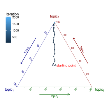
(a) AGS: $\bm{\pi}^{(2000)}_{1}=(\epsilon,.996,.003)$

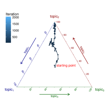
(b) MGS: $\bm{\pi}^{(2000)}_{1}=(.001,.997,\epsilon)$

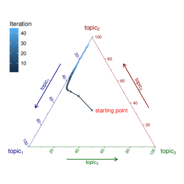
(c) VEM: $\bm{\pi}^{(45)}_{1}=(.057,.935,.006)$

Figure 13: Plots of values of $\bm{\pi}_{1}$ via algorithms AGS, MGS, and VEM. Here, the variable $\epsilon$ denotes a small number. With approximately $42$ iterations the AGS chain reached the optimal region, i.e., $.003$ from the true value $\bm{\pi}^{\text{true}}_{1}=(.002,\epsilon,.997)$, but the MGS chain took $248$ iterations to reach there. Algorithm VEM never reached the optimal regions: at convergence, VEM hit points that are $0.08$ far from $\bm{\pi}^{\text{true}}_{1}$. See discussion in the text.

We now compare the mixing rates of the two chains AGS and MGS. People often use diagnostics such as trace plots and auto-correlation function (ACF) plots for this purpose. Although both chains appear to converge in reasonable cycles, the AGS chain mixes faster as shown in Figure 13 and 3. Figure 14 further supports this fact: it gives plots of ACF’s for two random elements $\pi_{11}$ and $\pi_{22}$ of the $\bm{\pi}$ matrix, from each iteration of the chains AGS and MGS. These plots suggests that the AGS chain mixes faster, iterations separated by a lag of $25$ or $30$ are essentially uncorrelated. Note that even though the VEM algorithm did not reach the optimal regions here, in our experience, it converges relatively quickly. For modeling corpora with large document collections, we still recommend the reader to use the VEM algorithm as a practical alternative, considering its speed gains and parallelization capabilities. On the other hand, AGS gives more accurate results; hence, we use AGS for our future analysis.

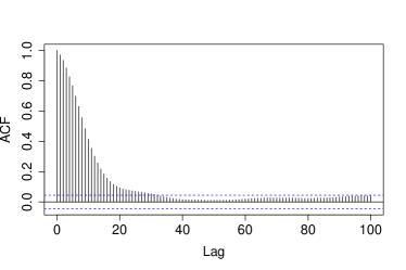
(a) $\pi_{11}$: AGS

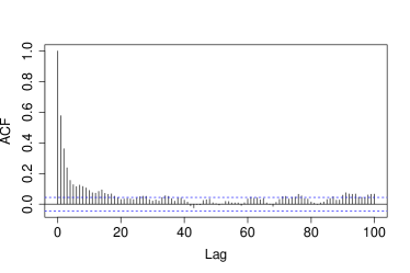
(b) $\pi_{22}$: AGS

(c) $\pi_{11}$: MGS

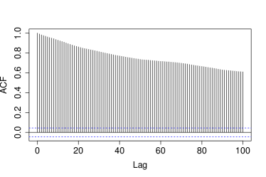
(d) $\pi_{22}$: MGS

Figure 14: Plots of ACF for samples $\pi_{11}$ and $\pi_{22}$ from the Markov chains MGS and AGS.

Note that sampling ${\bm{z}}$’s in both AGS and MGS chains is quite similar to sampling ${\bm{z}}$’s in the LDA CGS (Griffiths and Steyvers, 2004) chain. The CGS chain is a well-studied chain, see, e.g., George (2015); so, we do not report diagnostics for samples of ${\bm{z}}$ from the chains AGS and MGS here.

Appendix G Perplexity Calculation for cLDA and LDA

In this section, we derive expressions for Perplexity (defined in Section 4.2) for both cLDA and LDA models. To compute the perplexity score (21), we first need an expression for the predictive likelihood $p(w_{jdi}\,|\,{\bm{w}}^{\text{train}})$. We obtain this by marginalizing the likelihood over $\bm{\beta},\bm{\pi},\bm{\theta}$ and $z_{jdi}$. There is a slight abuse of notation here: the variables $\bm{\beta},\bm{\pi},\bm{\theta}$ are all dependent on the training data ${\bm{w}}^{\text{train}}$ only, but we ignore this in the notation. From the hierarchical model, we can write the predictive likelihood for word $w_{jdi}$ as

$$\ell_{w_{jdi}}(\bm{\beta},\bm{\theta}_{jd},z_{jdi})=\prod_{k=1}^{K}\prod_{v=1}^{V}\beta_{kv}^{z_{jdik}w_{jdiv}}=\sum_{k=1}^{K}z_{jdik}\prod_{v=1}^{V}\beta_{kv}^{w_{jdiv}}$$ (95)

where we used the property that $\prod_{k=1}^{K}\prod_{v=1}^{V}\beta_{kv}^{z_{jdik}w_{jdiv}}=\prod_{v=1}^{V}\beta_{k^{\prime}v}^{w_{jdiv}}$ for some $k^{\prime}$ such that $z_{jdik^{\prime}}=1$. The dependence of the likelihood on $\bm{\pi}_{j}$’s is ignored in the notation as it’s included in $\bm{\theta}_{jd}$’s. Since $z_{jdi}\sim\operatorname{Mult}_{K}(\bm{\theta}_{jd})$, $E(z_{jdi})=\theta_{jdk}$, for $j=1,\ldots,J$, $d=1,\ldots,D_{j}$, $i=1,\ldots,n_{jd}$ and $k=1,\ldots,K$. We then have

$$\begin{split}\ell_{w_{jdi}}(\bm{\beta},\bm{\theta}_{jd})&=E\Bigl{[}\sum_{k=1}^{K}z_{jdik}\prod_{v=1}^{V}\beta_{kv}^{w_{jdiv}}\Bigl{]}=\sum_{k=1}^{K}\Bigl{[}E(z_{jdik})\prod_{v=1}^{V}\beta_{kv}^{w_{jdiv}}\Bigl{]}\\ &=\sum_{k=1}^{K}\Bigl{[}\theta_{jdk}\prod_{v=1}^{V}\beta_{kv}^{w_{jdiv}}\Bigl{]}\\ \end{split}$$ (96)

Let $(\bm{\beta}^{[1]},\bm{\theta}^{[1]}),\ldots,(\bm{\beta}^{[S]},\bm{\theta}^{[S]})$ be a Markov chain with invariant distribution $\nu_{h,{\bm{w}}^{\text{train}}}(\bm{\beta},\bm{\theta})$. One can then estimate the marginal likelihood $p(w_{jdi}\,|\,{\bm{w}}^{\text{train}})$ in (21) by the Monte Carlo average

$$\frac{1}{S}\sum_{s=1}^{S}\sum_{k=1}^{K}\Bigl{[}\theta^{[s]}_{jdk}\prod_{v=1}^{V}{\beta^{[s]}}_{kv}^{w_{jdiv}}\Bigl{]}$$ (97)

We can use any of the augmented chains on $(\bm{\beta},\bm{\pi},\bm{\theta},{\bm{z}})$ described in Section 3.1 to compute this average. An elegant alternative is to substitute the following estimates of $\theta^{[s]}_{jdk}$ and ${\beta^{[s]}}_{kv}$ in (97)

$$\begin{split}\hat{\theta}^{[s]}_{jdk}&=E_{\bm{\pi}_{j},{\bm{z}}_{d},{\bm{w}}_{d}}\left(\theta^{[s]}_{jdk}\,|\,{\bm{z}}_{d},\bm{\pi}_{j},{\bm{w}}_{d}\right)=\frac{n_{jdk}^{\text{train}}+\gamma\bm{\pi}^{[s]}_{j}}{n_{jd.}^{\text{train}}+\gamma}\\ \hat{\beta}^{[s]}_{kv}&=E_{{\bm{z}},{\bm{w}}}\left(\beta^{[s]}_{kv}\,|\,{\bm{z}},{\bm{w}}\right)=\frac{m_{..kv}^{\text{train}}+\eta}{m_{..k.}^{\text{train}}+V\eta}\\ \end{split}$$ (98)

which can be computed for every sample in a chain on $(\bm{\pi},{\bm{z}})$. The resulting likelihood estimate dominates the original estimate (97) in terms of variance. This approach is sometimes called as Rao-Blackwellization, see, e.g., (Robert and Casella, 2005, Chapter 4). To compute these estimates, we only need a Markov chain on $(\bm{\pi},{\bm{z}})$, which has reduced computational cost compared to a Markov chain on $(\bm{\beta},\bm{\pi},\bm{\theta},{\bm{z}})$. Note that one can plug in variational estimates of $\theta_{jdk}$ and $\beta_{kv}$ via the cLDA variational EM algorithm (see Section E) into (96) to estimate the marginal likelihood $p(w_{jdi}\,|\,{\bm{w}}^{\text{train}})$.

Using similar arguments, we can derive an expression for the estimate of the marginal likelihood $p(w_{di}\,|\,{\bm{w}}^{\text{train}})$ for the LDA model. Given the CGS chain $z^{[1]},\ldots,z^{[S]}$ (Griffiths and Steyvers, 2004), we have

$$\hat{p}(w_{di}\,|\,{\bm{w}}^{\text{train}})=\frac{1}{S}\sum_{s=1}^{S}\sum_{k=1}^{K}\Bigl{[}\hat{\theta}^{[s]}_{dk}\prod_{v=1}^{V}{\hat{\beta}^{[s]}}_{kv}^{w_{div}}\Bigl{]},$$ (99)

where

$$\begin{split}\hat{\theta}^{[s]}_{dk}&=\frac{n_{dk}^{\text{train}}+\alpha}{n_{d.}^{\text{train}}+K\alpha}\\ \hat{\beta}^{[s]}_{kv}&=\frac{m_{.kv}^{\text{train}}+\eta}{m_{.k.}^{\text{train}}+V\eta}.\end{split}$$ (100)

Appendix H Additional Experimental Results

This section gives additional results of experiments on real world corpora that are discussed in Section 4.

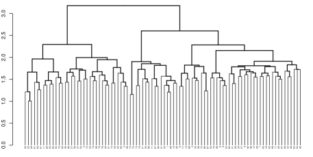
(a) cLDA topics: hclust dendrogram

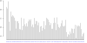
(b) cLDA topics’ size (log scale)

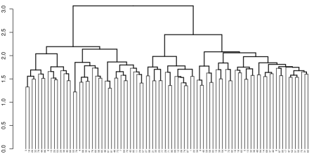
(c) LDA topics: hclust dendrogram

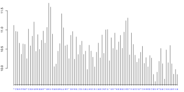
(d) LDA topics’ size (log scale)

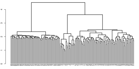
(e) HDP topics: hclust dendrogram

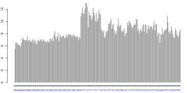
(f) HDP topics’ size (log scale)

Figure 15: Comparing topics learned via cLDA-AGS, LDA-CGS, and HDP-CRF algorithms. Left-column shows hclust dendrograms built from topic-to-topic similarity matrices calculated based on the manhattan distance for all three algorithms. For each method, right-column shows barplots of topic-sizes (i.e. the total number of words assigned to a topic). Topics in the barplot $x$-axis were ordered based on the order of topics in the corresponding dendrogram leaf-nodes to ease comparison. HDP found redundant set of topics and many topics with too low topic-size—e.g. the children of the first/left child in the dendrogram in Plot (e). See discussion in Section 4.2.

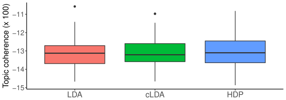
Figure 17: Estimated topic coherences for models LDA, cLDA, and HDP for corpus NIPS $00$-$18$. See discussion in Section 4.2.

(a) topic $3$ (Science)

(b) topic $10$ (Uninformative)

(c) topic $21$ (Recreation)

(d) topic $13$ (Computers)

(e) topic $28$ (Politics, gun trade)

(f) topic $29$ (Computers)

Figure 19: $20$ most probable words for three selected topics from a $30$-topic cLDA model trained on corpus $16$newsgroups. The $x$-axis gives the corresponding (estimated) probabilities of words given a topic.

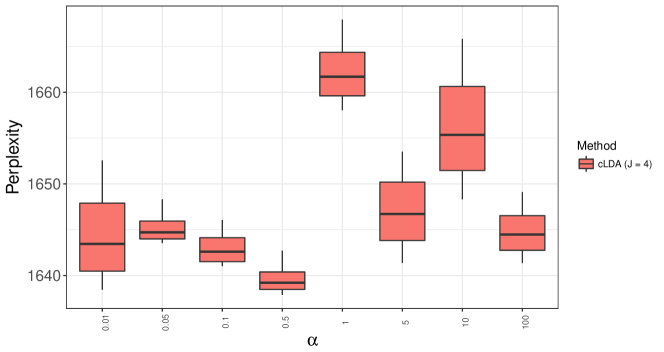
Figure 20: Boxplots of perplexity scores of cLDA models with various values of $\alpha$ keeping $\eta$ and $\gamma$ fixed, for corpus NIPS $00$-$18$.

References

- Abramowitz (1974) Milton Abramowitz. Handbook of Mathematical Functions, With Formulas, Graphs, and Mathematical Tables,. Dover Publications, Incorporated, 1974. ISBN 0486612724.
- Aldous (1985) David J. Aldous. Exchangeability and related topics. In École d’été de probabilités de Saint-Flour, XIII—1983, volume 1117 of Lecture Notes in Math., pages 1–198. Springer, Berlin, 1985.
- Besag (1994) Julian Besag. Discussion: Markov chains for exploring posterior distributions. The Annals of Statistics, 22(4):1734–1741, 12 1994.
- Bishop et al. (2006) Christopher M Bishop et al. Pattern Recognition and Machine Learning, volume 1. Springer, New York, 2006.
- Blei et al. (2003) David M. Blei, Andrew Y. Ng, and Michael I. Jordan. Latent Dirichlet allocation. Journal of Machine Learning Research, 3:993–1022, 2003.
- Blei et al. (2004) David M. Blei, Thomas L. Griffiths, Michael I. Jordan, and Joshua B. Tenenbaum. Hierarchical topic models and the nested chinese restaurant process. In Advances in Neural Information Processing Systems, page 2003. MIT Press, 2004.
- Deerwester et al. (1990) Scott Deerwester, Susan T Dumais, George W Furnas, Thomas K Landauer, and Richard Harshman. Indexing by latent semantic analysis. Journal of the American society for information science, 41(6):391, 1990.
- Dempster et al. (1977) A. P. Dempster, N. M. Laird, and D. B. Rubin. Maximum likelihood from incomplete data via the EM algorithm (C/R: p22–37). Journal of the Royal Statistical Society, Series B, 39:1–22, 1977.
- Ferguson (1973) Thomas S. Ferguson. A Bayesian analysis of some nonparametric problems. The Annals of Statistics, 1:209–230, 1973.
- Ferguson (1974) Thomas S. Ferguson. Prior distributions on spaces of probability measures. The Annals of Statistics, 2:615–629, 1974.
- George (2015) Clint P. George. Latent Dirichlet Allocation: Hyperparameter Selection and Applications to Electronic Discovery. PhD thesis, University of Florida, 2015.
- Girolami and Calderhead (2011) Mark Girolami and Ben Calderhead. Riemann manifold langevin and hamiltonian monte carlo methods. Journal of the Royal Statistical Society: Series B (Statistical Methodology), 73(2):123–214, 2011. ISSN 1467-9868.
- Globerson et al. (2007) A. Globerson, G. Chechik, F. Pereira, and N. Tishby. Euclidean Embedding of Co-occurrence Data. Journal of Machine Learning Research, 8:2265–2295, 2007.
- Griffiths and Steyvers (2004) Thomas L. Griffiths and Mark Steyvers. Finding scientific topics. Proceedings of the National Academy of Sciences, 101:5228–5235, 2004.
- Hastings (1970) W. K. Hastings. Monte Carlo sampling methods using Markov chains and their applications. Biometrika, 57:97–109, 1970.
- Hofmann (1999) Thomas Hofmann. Probabilistic latent semantic indexing. In Proceedings of the 22Nd Annual International ACM SIGIR Conference on Research and Development in Information Retrieval, SIGIR ’99, pages 50–57, New York, NY, USA, 1999. ACM. ISBN 1-58113-096-1.
- Jordan et al. (1999) Michael I. Jordan, Zoubin Ghahramani, Tommi S. Jaakkola, and Lawrence K. Saul. An introduction to variational methods for graphical models. Machine Learning, 37(2):183–233, 1999. ISSN 1573-0565.
- Kennedy (1990) A. D. Kennedy. Probabilistic Methods in Quantum Field Theory and Quantum Gravity, chapter The Theory of Hybrid Stochastic Algorithms, pages 209–223. Springer US, Boston, MA, 1990. ISBN 978-1-4615-3784-7.
- Kim et al. (2013) Do-kyum Kim, Geoffrey Voelker, and Lawrence K Saul. A variational approximation for topic modeling of hierarchical corpora. In Proceedings of the 30th International Conference on Machine Learning (ICML-13), pages 55–63, 2013.
- Mcauliffe and Blei (2008) Jon D Mcauliffe and David M Blei. Supervised topic models. In Advances in neural information processing systems, pages 121–128, 2008.
- Metropolis et al. (1953) N. Metropolis, A. W. Rosenbluth, M. N. Rosenbluth, A. H. Teller, and E. Teller. Equations of state calculations by fast computing machines. Journal of Chemical Physics, 21:1087–1091, 1953.
- Mimno et al. (2011) David Mimno, Hanna M Wallach, Edmund Talley, Miriam Leenders, and Andrew McCallum. Optimizing semantic coherence in topic models. In Proceedings of the conference on empirical methods in natural language processing, pages 262–272. Association for Computational Linguistics, 2011.
- Minka (2000a) Thomas Minka. Estimating a dirichlet distribution, 2000a.
- Minka (2000b) Thomas P. Minka. Beyond Newton’s method. Technical report, Microsoft, 2000b.
- Neal (2000) Radford M. Neal. Markov chain sampling methods for Dirichlet process mixture models. Journal of Computational and Graphical Statistics, 9:249–265, 2000.
- Neal (2010) Radford M. Neal. MCMC using Hamiltonian dynamics. Handbook of Markov Chain Monte Carlo, 54:113–162, 2010.
- Newman et al. (2009) David Newman, Arthur U. Asuncion, Padhraic Smyth, and Max Welling. Distributed algorithms for topic models. Journal of Machine Learning Research, 10:1801–1828, 2009.
- Patterson and Teh (2013) Sam Patterson and Yee Whye Teh. Stochastic Gradient Riemannian Langevin Dynamics on the Probability Simplex. Advances in Nueral Information Processing Systems 26 (Proceedings of NIPS), pages 1–10, 2013. ISSN 10495258.
- Robert and Casella (2005) Christian P. Robert and George Casella. Monte Carlo Statistical Methods (Springer Texts in Statistics). Springer-Verlag New York, Inc., Secaucus, NJ, USA, 2005. ISBN 0387212396.
- Roberts and Tweedie (1996) Gareth O. Roberts and Richard L. Tweedie. Exponential convergence of langevin distributions and their discrete approximations. Bernoulli, 2(4):341–363, 1996. ISSN 13507265.
- Salton et al. (1975) G. Salton, A. Wong, and C. S. Yang. A vector space model for automatic indexing. Commun. ACM, 18(11):613–620, November 1975. ISSN 0001-0782.
- Teh et al. (2006) Y. W. Teh, M. I. Jordan, M. J. Beal, and D. M. Blei. Hierarchical Dirichlet processes. Journal of the American Statistical Association, 101:1566–1581, 2006.
- Teh et al. (2007) Yee W. Teh, David Newman, and Max Welling. A collapsed variational bayesian inference algorithm for latent dirichlet allocation. In B. Schölkopf, J. C. Platt, and T. Hoffman, editors, Advances in Neural Information Processing Systems 19, pages 1353–1360. MIT Press, 2007.
- Wallach (2006) Hanna M. Wallach. Topic modelling: beyond bag-of-words. In Proceedings of the International Confernce on Machine Learning, pages 977–984, 2006.
- Wallach et al. (2009a) Hanna M. Wallach, David Mimno, and Andrew McCallum. Rethinking LDA: Why priors matter. Advances in Neural Information Processing Systems, 22:1973–1981, 2009a.
- Wallach et al. (2009b) Hanna M Wallach, Iain Murray, Ruslan Salakhutdinov, and David Mimno. Evaluation methods for topic models. In Proceedings of the 26th Annual International Conference on Machine Learning, pages 1105–1112. ACM, 2009b.
- Wallach et al. (2009c) Hanna M Wallach, Iain Murray, Ruslan Salakhutdinov, and David Mimno. Evaluation methods for topic models. In Proceedings of the 26th Annual International Conference on Machine Learning, pages 1105–1112. ACM, 2009c.
- Zhai et al. (2004) ChengXiang Zhai, Atulya Velivelli, and Bei Yu. A cross-collection mixture model for comparative text mining. In Proceedings of the Tenth ACM SIGKDD International Conference on Knowledge Discovery and Data Mining, KDD ’04, pages 743–748, New York, NY, USA, 2004. ACM. ISBN 1-58113-888-1.
- Zhu and Xing (2014) Jun Zhu and Eric P Xing. Discriminative training of mixed membership models., 2014.