Using binary decision diagrams for constraint handling in combinatorial interaction testing

Abstract

Constraints among test parameters often have substantial effects on the performance of test case generation for combinatorial interaction testing. This paper investigates the effectiveness of the use of Binary Decision Diagrams (BDDs) for constraint handling. BDDs are a data structure used to represent and manipulate Boolean functions. The core role of a constraint handler is to perform a check to determine if a partial test case with unspecified parameter values satisfies the constraints. In the course of generating a test suite, this check is executed a number of times; thus the efficiency of the check significantly affects the overall time required for test case generation. In the paper, we study two different approaches. The first approach performs this check by computing the logical AND of Boolean functions that represent all constraint-satisfying full test cases and a given partial test case. The second approach uses a new technique to construct a BDD that represents all constraint-satisfying partial test cases. With this BDD, the check can be performed by simply traversing the BDD from the root to a sink. We developed a program that incorporates both approaches into IPOG, a well-known test case generation algorithm. Using this program, we empirically evaluate the performance of these BDD-based constraint handling approaches using a total of 62 problem instances. In the evaluation, the two approaches are compared with three different constraint handling approaches, namely, those based on Boolean satisfiability (SAT) solving, Minimum Forbidden Tuples (MFTs), and Constraint Satisfiction Problem (CSP) solving. The results of the evaluation show that the two BDD-based approaches usually outperform the other constraint handling techniques and that the BDD-based approach using the new technique exhibits best performance.

1 Introduction

In testing of real-world systems, executing all possible test cases is impractical, as the number of the test cases is usually prohibitively large. This motivates the development of cost reduction strategies. Combinatorial Interaction Testing (CIT) (Grindal et al., 2005; Nie and Leung, 2011; Kuhn et al., 2013) is one of these testing strategies. CIT requires the tester to test all parameter interactions of interest, rather than all possible test cases. The most basic and well-practiced form of CIT is $t$-wise testing. This strategy requires testing all value combinations among any $t$ parameters. Previous studies show that small $t$ is often sufficient to detect a significant percentage of defects (Kuhn et al., 2004). Hence this can greatly reduce the number of test cases to execute. The value $t$ is usually referred to as strength.

Figure 1 shows an example of a test suite for $t=2$. The System Under Test (SUT) assumed here is a printer. The SUT model has three parameters: Paper size, Feed tray, and Paper type. The set of possible values for these parameters are: {B4, A4, B5}, {Bypass, Tray 1, Tray 2}, and {Thick, Normal, Thin}. As can be seen from the figure, every pair-wise combination occurs in at least one of the test cases in the test suite. Note that the test suite is much smaller than the exhaustive test suite, which contains $3\times 3\times 3=27$ test cases.

Paper size	Feed tray	Paper type
B4	Bypass	Thick
B4	Tray 1	Thin
B4	Tray 2	Normal
A4	Bypass	Normal
A4	Tray 1	Thick
A4	Tray 2	Thin
B5	Bypass	Thin
B5	Tray 1	Normal
B5	Tray 2	Thick

Figure 1: Test suite of strength $t=2$. No constraints are considered.

This SUT example implicitly assumes that every possible test case can be executed. Real-world systems, however, often have constraints concerning executable test cases. In such a case, all test cases must satisfy the given constraints to execute. In addition, some interactions may become inherently not testable. Constraint handling is necessary to solve these problems in the process of test case generation. Though this might look an easy task, the efficiency of constraint handling sometimes greatly affects the whole performance of test case generation.

It is easy to decide whether a test case satisfies the constraints, because it suffices to check if the test case satisfies each constraint one by one. The difficulty of constraint handling stems from the need to determine whether an interaction can be testable or not, or equivalently whether an incomplete test case with unspecified values can be extended to a full-fledged test case that satisfies the constraints. For example, consider the following constraints.

• If the Paper size is B4, then the Feed tray must be Bypass.

• If the Feed tray is Bypass, then the Paper type must not be Thick.

In this case, B4 and Thick cannot occur in the same test case and thus their interaction is not testable, because B4 requires Bypass which in turn prohibits Thick. However, this cannot be decided by analyzing each of the two constraints in isolation. We say that an interaction (partial test case) or test case is invalid if it cannot be tested due to the constraints.

When constructing a test suite for CIT, such validity checks need to be performed a large number of times. As a result, the time used for validity checks is often dominant in the whole running time required to generate a test suite. Although modern test case generation tools are usually able to handle real-world problems in practical running times, problems sometimes arise that take very long time to solve because of complex constraints. The existence of such hard problems can severely hinder the practical usefulness of CIT.

In fact, we started our study on constraint handling in response to the demand from our industry collaborators who were not satisfied with a test case generation tool that was then popular. Their complaint was that the execution time of the tool was sometimes too long to be useful in practice, especially the SUT involves many constraints. To achieve better performance, we adopted Binary Decision Diagrams (BDDs) (Akers, 1978; Bryant, 1986) as a key data structure on which constraint handling is performed. A BDD is a data structure that can compactly represent a Boolean function. We developed a test generation tool named CIT-BACH using BDDs. Our attempt was successful in the sense that our tool has been used in industry for years. However, the performance of BDD-based constraint handling has not been systematically evaluated so far. Because of the lack of studies, it has been not clear whether BDDs are indeed useful or other approaches perform better.

Aimed at filling this lack, this paper first 1) describes the BDD-based constraint handling approaches and then 2) compares the performance between these BDD-based approaches and other approaches. We consider two different BDD-based approaches. The first approach is a natural and straightforward one. It performs the check by computing the conjunction of Boolean functions representing the constraints and the given partial test case. The second approach uses the algorithm that we developed for constraint handling in the CIT-BACH tool. In this approach, a BDD is constructed that represents all valid full and partial test cases. Once such a BDD has been created, the check can be performed simply by traversing the BDD from the root node to a terminal node, thus avoiding any further BDD operations. Although the basic form of this approach has been used in our tool for some years, this paper describes it for the first time, together with some optimization techniques.

To compare these approaches with other constraint handling approaches, we developed a new program that combines the IPOG algorithm (Lei et al., 2007, 2008) and the BDD-based constraint handling approaches. The IPOG algorithm is a well-known test suite generation algorithm and adopted by ACTS (Yu et al., 2013a), one of the state-of-the-art tools. Since our program and ACTS shares the same algorithm except in constraint handling, using the two programs allows us to compare the BDD-based constraint handling approaches and other approaches employed by ACTS. We conducted an experiment campaign where we applied the two tools to a collection of various problem instances. This collection includes 62 problem instances, all taken from previous studies in the field of CIT except one that was provided by our industry collaborators.

The rest of the paper is organized as follows. Section 2 describes the model of SUTs. Section 3 describes the outline of test case generation algorithms and how constraint handling is needed in the process of test case generation. Section 4 shows how to represent the set of valid test cases using a BDD. Section 5 describes the two BDD-based constraint handling approaches which use the BDD representation of valid test cases described in Section 4. Section 6 presents the results of experiments. Section 7 presents a concise survey of related work. Section 8 describes the potential threats to validity. Finally we conclude this paper in Section 9.

2 Model

We assume that the SUT has $n$ parameter variables (or parameters for short), $P_{1},...,P_{n}$. Parameter variable $P_{i}$ has its finite domain $D_{i}$ from which a value for the parameter is drawn. For simplicity of presentation, we assume that $D_{i}=\{0,1,...,|D_{i}|-1\}$.

A test case is an $n$-tuple such that its $i$th element is a value for $P_{i}$. Hence the set of test cases is $D_{1}\times D_{2}\times...\times D_{n}$.

In practice, a test case may need to satisfy some condition to be executed. Constraints over parameter values mean such a condition. The constrains are formally represented as a Boolean-valued function $F$ over the parameter variables:

$$F:D_{1}\times D_{2}\times...\times D_{n}\rightarrow\{0,1\}$$

where a test case $t$ satisfies the constraints if and only if $F(t)=1$. We say that a test case is valid if and only if it satisfies the constraints. We assume that $F$ is given as a formula composed of the Boolean connectives (such as $\neg$, $\land$, $\lor$ and $\Rightarrow$) and terms in the forms of $P_{i}=v\ (v\in D_{i})$ and $P_{i}=P_{j}$.

For instance, the SUT model shown in Section 1 is expressed using $n=3$ parameter variables $P_{1},P_{2},P_{3}$ which respectively represent Paper size, Feed tray and Paper type. The domains of the parameter variables are $D_{1},D_{2}$ and $D_{3}$ where $D_{1}=D_{2}=D_{3}=\{0,1,2\}$. We assume that each integer in the domains corresponds to a parameter value as follows:

$D_{1}$	0: B4	1: A4	2: B5
$D_{2}$	0: Bypass	1: Tray 1	2: Tray 2
$D_{3}$	0: Thick	1: Normal	2: Thin

The Boolean-valued function representing the constraints of the example is as follows:

$$F:=(P_{1}=0\Rightarrow P_{2}=0)\land(P_{2}=0\Rightarrow\neg(P_{3}=0))$$

A test case is a vector of length 3 whose element is either 0, 1 or 2. For example, (1, 0, 2) or (2, 0, 0) are test cases. The former test case is valid, whereas the latter is not valid.

Paper size	Feed tray	Paper type
Bypass	B4	Thin
Bypass	A4	Normal
Tray1	A4	Thick
Tray2	A4	Thin
Bypass	B5	Normal
Tray1	B5	Thin
Tray2	B5	Thick
$-$	B4	Normal
Tray1	$-$	Normal
Tray2	$-$	Normal

Figure 2: Test suite constructed by IPOG for the running example (strength $t=2$). Although there are three partial test cases, all pairwise interactions have already been covered. The process of assigning values to the entries with a $-$ is omitted in Figure 3 for simplicity.

1:  Sort the parameters in non-increasing order of $|D_{i}|$  {For simplicity we assume $P_{1},...,P_{n}$ are sorted in this order.}

2:  $TestSuite\leftarrow\emptyset$

3:  {Cover all value combinations of the first $t$ parameters}

4:  for each combination $I$ of values of the first $t$ parameters do

5:     if isValid($I$) then

6:        $TestSuite\leftarrow TestSuite\cup\{T\}$

7:     end if

8:  end for

9:  {Add remaining $n-t$ parameters}

10:  for each $i=t+1,...,n$ do

11:     {Enumerate valid $t$-way value combinations of $P_{i}$ and $P_{i_{1}},...,P_{i_{t-1}}$}

12:     $\pi\leftarrow\emptyset$

13:     for each $t$-way combination $I$ of values of $P_{i}$ and $P_{i_{1}},...,P_{i_{t-1}}$ such that $1\leq i_{1}<...<i_{t-1}\leq i-1$ do

14:        if isValid($I$) then

15:           $\pi\leftarrow\pi\cup\{I\}$

16:        end if

17:     end for

18:     {Horizontal growth}

19:     for each $T=(v_{1},..,v_{i-1})$ in $TestSuite$ do

20:        Choose a value $v_{i}$ of $P_{i}$ and replace $T$ with $T^{\prime}=(v_{1},...,v_{i-1},v_{i})$ so that isValid($T^{\prime}$)=true and $T^{\prime}$ covers the most number of combinations of values in $\pi$

21:        Remove the combinations of values covered by $T^{\prime}$ from $\pi$

22:     end for

23:     {Vertical growth}

24:     for each combination $I$ in $\pi$ do

25:        if there exists $T\in TestSuite$ that can be changed to $T^{\prime}$ such that it covers both $T$ and $I$ and isValid($T^{\prime}$)=true then

26:           Replace $T\in TestSuite$ with $T^{\prime}$

27:        else

28:           $TestSuite\leftarrow TestSuite\cup\{I\}$

29:        end if

30:     end for

31:  end for

Figure 3: IPOG-C algorithm (based on (Yu et al., 2013b))

In addition to full test cases, we often need to consider “incomplete” test cases where there are some parameters whose value is yet to be fixed. We call such a vector a partial test case. More precisely, a partial test case is an $n$-tuple such that 1) the $i$th element is either a value in $D_{i}$ or special symbol $-$ representing that the value is unspecified, and 2) at least one parameter has a $-$. A partial test case $t$ is valid if and only if $t$ can be extended to a valid test case by assigning values to all the positions on which $-$ is placed. For example, $(1,1,-)$ and $(0,-,0)$ are partial test cases for the running example. The former partial test case is valid. On the other hand, the latter one is not valid (invalid), as explained in Section 1.

3 IPOG test case generation algorithm

Algorithms for constructing test suites for CIT have been widely studied. Roughly they can be classified into two groups: mathematical and computational. Mathematical algorithms use properties of mathematical elements, such as finite fields, to generate test suites. Basically it is difficult for these algorithms to deal with SUTs with constraints. As a result, there are only few test generation tools that use this group of algorithms.

Test case generation tools that have industrial strength usually use computational algorithms. In this paper we focus on IPOG (Lei et al., 2007, 2008), because ACTS (Yu et al., 2013a), which is a state-of-the art test generation tool for CIT, uses this algorithm. As described in Section 6, we develop a program that employs IPOG and constraint handling techniques using BDDs. This allows us to compare BDD-based techniques with different constraint handling techniques that are adopted by ACTS.

To be precise, the IPOG algorithm is not a single algorithm; rather it encompasses a few variants. The IPOG algorithm with the constraint handling capability is called IPOG-C (Yu et al., 2013b); however, as our concern here is about constraint handling, we call IPOG-C simply IPOG. Figure 3 shows the pseudo-code of this algorithm. The algorithm constructs a test suite as follows. It starts with a set of $t$ parameters and constructs a test suite for that parameter set (lines 3–8). Then, it adds a new parameter and decides a value on that parameter for every existing test case (horizontal growth, lines 18–22). If some $t$-way combinations are still missing in the test suite, the algorithm adds new test cases to the test suite to cover all such combinations (vertical growth, lines 23–30). As a result of iterating horizontal growth and vertical growth for all remaining parameters, a test suite for all parameters will be eventually constructed. Figure 2 show the test suite constructed by our IPOG implementation for the running example.

In this pseudo-code, we specify the points where constraint handling is called for by function isValid(). This function takes a full or partial test case $t$ as an argument and returns true if $t$ is valid; it returns false, otherwise. Note that in Figure 3, a value combination of parameters is treated as a partial test case that covers the combination and has a $-$ on all remaining parameters.

As can be seen in Figure 3, the validity check is performed a number of times in the process of constructing a single test suite: All $t$-way combinations of parameter values need to undergo the validity check (lines 3–8, 13–17). In addition, when deciding a value on parameter $P_{i}(i>t)$ of a test case, the validity check is performed (lines 20 and 25). Of course, some optimization can be made. For example, no validity check is required for any interaction among a subset of parameters if none of these parameters occur in the constraints. Although such optimizations are possible, the efficiency of constraint handling still has substantial effects on the performance of test case generation. In Section 6 we show this through experiments.

4 BDD representations of valid test cases

In this section, we describe the concept of a BDD and how it can be used to represent the set of valid test cases. The BDD representation of valid test cases provides the basis for the validity checking approaches described in Section 5.

4.1 Binary Decision Diagrams

A BDD is a data structure that represents a Boolean function (Bryant, 1986). It is a rooted directed acyclic graph with two types of nodes, terminal nodes and nonterminal nodes. Each nonterminal node is associated with a Boolean variable and has two successor nodes. Each edge is labeled by either 0 or 1. A terminal node is labeled by F (false) or T (true). A BDD is ordered if the Boolean variables occur in the same order along any path from the root to one of the terminal nodes. An ordered BDD can be transformed into a reduced ordered BDD (ROBDD) by repeatedly applying reduction rules until no further applications are possible. The application of these reduction rules removes all redundant isomorphic subgraphs and non-terminal nodes whose successor nodes are identical. For example, there are no more than two terminal nodes in an ROBDD. When the ordering of Boolean variables is fixed, an ROBDD is unique for a given Boolean function. Although there are several variants of BDDs, ROBDDs are now almost a synonym of BDDs; thus we call an ROBDD simply a BDD.

Figures 4 and 5 schematically show BDDs for Boolean functions with six variables $x_{1},x_{2},...,x_{6}$. Edges labeled by 0 are represented as dotted lines, whereas those labeled by 1 are represented as solid lines.

Given a valuation of the Boolean variables, that is, an assignment of truth values to the Boolean variables, the value of the Boolean function for the valuation is determined by traversing the BDD from the root according to the valuation. Specifically, when the current visiting node is associated with a Boolean variable $x_{i}$ and $x_{i}$ takes 0 (or 1) in the valuation, then the traversal proceeds by taking the edge labeled by 0 (or 1) to one of its successor nodes. If the terminal node reached is labeled by F (or T), then the value of the function is 0 (or 1). This check takes time linear in the length of the traversed path which is at most equal to the number of the Boolean variables.

From two BDDs that represent Boolean functions $b$ and $b^{\prime}$, another BDD that represents Boolean function $b\langle op\rangle b^{\prime}$ can be obtained with the algorithm $Apply$ (Bryant, 1986), where $\langle op\rangle$ can be any binary Boolean connective, such as $\land$ and $\lor$. The time complexity of $Apply$ is at most linear in the product of the numbers of nodes in the BDD representations of $b$ and $b^{\prime}$. The negation of a Boolean formula can be obtained even easier: it suffices to swap the two terminal nodes.

4.2 Constructing a BDD that represents the set of valid test cases

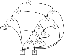
Figure 4: BDD representing the set of valid test cases. The dotted lines and solid lines represent edges labeled with 0 and edges labeled with 1.

Figure 4 shows a BDD representing the set of valid test cases for the running example. Here the value of each parameter $P_{i}$ is represented by two Boolean variables $x_{2i-1}$ and $x_{2i}$ with $x_{2i-1}$ being the least significant bit. For example, consider test cases $(1,0,2)$ and $(2,0,0)$, which represent (A4, Bypass, Thin) and (B5, Bypass, Thick), respectively. These test cases are represented by $x_{1},...,x_{6}$ as follows.

$$(1,0,2):\underbrace{10}_{x_{1}x_{2}}\underbrace{00}_{x_{3}x_{4}}\underbrace{01}_{x_{5}x_{6}}\quad(2,0,0):\underbrace{01}_{x_{1}x_{2}}\underbrace{00}_{x_{3}x_{4}}\underbrace{00}_{x_{5}x_{6}}$$

Here we write the least significant bit at the leftmost end for each parameter so that the above ordering of the Boolean variables can coincide with that of the BDD. Whether a test case is valid or not can be easily determined by traversing the BDD from the root node according to the 0-1 values of these Boolean variables.

It should be noted that this BDD provides the Boolean function representation of $F$, i.e., the function that determines valid test cases (see Section 2). We let $f$ denote this Boolean function. This function is of the form: $f:\{0,1\}^{M}\rightarrow\{0,1\}$, where $M$ is the number of Boolean variables. This function is obtained by computing the logical AND of the Boolean functions representing the condition that the value for $P_{i}$ is less than $|D_{i}|$ and the Boolean function representation of the SUT’s constraints among the parameter values.

The Boolean function representing $P_{i}<|D_{i}|$ is obtained from the binary representation of $|D_{i}|-1$. For example, suppose that $D_{i}=\{0,1,2\}$. Then $D_{i}$ is represented by two Boolean variables: $x_{i1}$ and $x_{i2}$. From the binary representation of 2, i.e., 10, one can derive the following function to ensure that the value for $P_{i}$ is at most 2.

$$x_{i2}\Rightarrow\neg x_{i1}$$

The given SUT’s constraints are straightforwardly represented as a Boolean function, because the Boolean function can be obtained by simply converting the constraints into binary representation. For example, consider the running example. Constraint $P_{1}=0\Rightarrow P_{2}=0$ is represented as

$$\neg x_{1}\neg x_{2}\Rightarrow\neg x_{3}\neg x_{4}$$

Similarly, $P_{2}=0\Rightarrow\neg(P_{3}=0)$ is represented as:

$$\neg x_{3}\neg x_{4}\Rightarrow\neg(\neg x_{5}\neg x_{6})$$

As a result, the set of valid test cases defined by $F$ is represented as the following Boolean function $f$.

$$\begin{array}[]{ll}&(x_{2}\Rightarrow\neg x_{1})\land(x_{4}\Rightarrow\neg x_{3})\land(x_{6}\Rightarrow\neg x_{5})\\ \land&(\neg x_{1}\neg x_{2}\Rightarrow\neg x_{3}\neg x_{4})\\ \land&(\neg x_{3}\neg x_{4}\Rightarrow\neg(\neg x_{5}\neg x_{6}))\end{array}$$

The BDD shown in Figure 4 exactly represents this Boolean function. All these operations over Boolean functions can be performed by manipulating their BDD representations.

5 Checking the validity of partial test cases

As stated in the previous section, once the BDD representing the set of all valid test cases has been constructed, whether a given test case is valid or not can be easily checked by traversing the BDD from the root according to the binary representation of the test case. On the other hand, the check whether a partial test case is valid or not cannot be performed only by traversing the BDD.

In this section, we present two approaches to validity checking for partial test cases. The first approach is natural and straightforward. It computes the conjunction, that is, logical AND of Boolean functions representing the constraints and the given partial test case and then checks if the Boolean function represented by the resulting BDD is a constant false, in which case the partial test case is invalid.

The second one is a novel approach. In the approach, the BDD representing the space of valid test cases is modified so that it can represent both valid test cases and valid partial test cases. As a result, the validity of partial test cases can be checked by traversing the BDD from the root to the terminal nodes, just in the same way as the validity of full test cases are determined.

5.1 Approach 1: ANDing Boolean functions

The first approach requires building another BDD that represents a given partial test case and performing the AND operation over the BDD and the BDD representing $f$ (i.e., the BDD representing the set of valid test cases). If the resulting BDD represents a contradiction (constant false), then the partial test case is invalid; otherwise, it is valid. The number of Boolean variables used in this approach is $\sum_{i=1}^{n}\lceil\log_{2}|D_{i}|\rceil$.

The Boolean function that represents a partial test case is constructed by ANDing the binary representations of the parameter values that have already been fixed. For example, consider two partial test cases as follows:

$$(1,1,-):\underbrace{10}_{x_{1}x_{2}}\underbrace{10}_{x_{3}x_{4}}\underbrace{--}_{x_{5}x_{6}}\quad(0,-,0):\underbrace{00}_{x_{1}x_{2}}\underbrace{--}_{x_{3}x_{4}}\underbrace{00}_{x_{5}x_{6}}$$

Note again that we write the least significant bit at the leftmost end for each parameter. The Boolean functions that represent these partial test cases are:

$$(1,1,-):x_{1}\neg x_{2}x_{3}\neg x_{4}\quad(0,-1,0):\neg x_{1}\neg x_{2}\neg x_{5}\neg x_{6}$$

Let $f_{T}$ be a Boolean function representing a partial test case $T$. Since the Boolean function $f_{T}\land f$ represents the set of valid test cases that cover $T$, the validity check of $T$ can be implemented as follows:

$$\mathtt{isValid(}T\mathtt{)}=\left\{\begin{array}[]{cl}false&f_{T}\land f=\mathrm{constant\ false}\\ true&\mathrm{otherwise}\end{array}\right.$$

The BDD representing a constant false consists only of a single terminal node which is labeled with F; thus the time complexity of checking if the resulting BDD represents a constant false or not is $O(1)$. The worst-case time complexity of computing $f_{T}\land f$ is linear in the product of the sizes of the two BDDs. However, in practice the computation time is usually small, because $f_{T}$ has a very simple BDD representation, where there are only as many non-terminal nodes as Boolean variables occurring in $f_{T}$. In Section 6, we experimentally evaluate the performance of this approach.

5.2 Approach 2: Constructing a BDD representing partial test cases

5.2.1 Outline

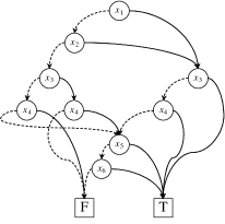
Figure 5: BDD representing all valid full and partial test cases

The fundamental idea of this approach is to construct a BDD that represents the set of all valid full/partial test cases. This allows us to determine very quickly whether a given partial test case is valid or not.

Now consider extending the domain $D_{i}$ of parameter $P_{i}$ by adding the element $-$ which represents that the value of the parameter is unspecified. Then the set of valid full and partial test cases is represented in the form of a Boolean-valued function as follows:

$$G:D_{1}\cup\{-\}\times D_{2}\cup\{-\}\times...\times D_{n}\cup\{-\}\rightarrow\{0,1\}$$

where a full or partial test case $T$ is valid if and only if $V(T)=1$.

To encode the domain of the function $V$ in bit strings, the special value $-$ is represented as $11...1$, whereas the values in $D_{i}$ are represented in the usually binary form, just as in the ordinary BDD representation.

Figure 5 shows the BDD that represents $G$ for the running example. Partial test cases are represented using valuations to Boolean variables $x_{1},...,x_{6}$, just as full test cases. Below are examples.

$$(1,1,-):\underbrace{10}_{x_{1}x_{2}}\underbrace{10}_{x_{3}x_{4}}\underbrace{11}_{x_{5}x_{6}}\quad(0,-,0):\underbrace{00}_{x_{1}x_{2}}\underbrace{11}_{x_{3}x_{4}}\underbrace{00}_{x_{5}x_{6}}$$

Given a binary representation of a test case or partial test case, checking if it is valid or not can be done simply by traversing the BDD from the root node to one of the terminal nodes. The time required for the validity check based on the BDD is linear in the length of the traversed path. As the path length is at most the number of Boolean variables, the time required for the validity check is linear in the number of parameters and logarithmic in the number of values of possible parameter values.

5.2.2 Constructing a BDD representing valid full and partial test cases

1:  $g$ $\leftarrow$ $f$: Boolean function that represents $F$  {Initially $g$ represents the set of all valid full test cases.}

2:  for each parameter variable $P_{i}$ do

3:     $cube$ $\leftarrow$ $x_{M_{i-1}+1}x_{M_{i-1}+2}...x_{M_{i}}$  {$x_{M_{i-1}+1},...,x_{M_{i}}$ are the Boolean variables representing $P_{i}$.}

4:     $tmp$ $\leftarrow$ $Exists(cube,g)$  {$tmp=\exists x_{M_{i-1}+1}...\exists x_{M_{i}}g$}

5:     $h$ $\leftarrow$ $Apply(\land,tmp,cube)$;  {$h=\exists x_{M_{i-1}+1}...\exists x_{M_{i}}g\ \land\ x_{M_{i-1}+1}x_{M_{i-1}+2}...x_{M_{i}}$}

6:     $g$ $\leftarrow$ $Apply(\lor,f,h)$  {$g$ is replaced with $g\lor h$}

7:  end for

Figure 6: BDD modification algorithm. The algorithm converts the BDD representing $F$ into another BDD representing $G$, where $F$ and $G$ respectively express the set of valid full test cases and the set of valid full and partial test cases.

Below we show how to construct the BDD that represents the set of all valid full and partial test cases. This process consists of two steps. In the first step, the BDD that represents $F$, or equivalently the set of all valid full test cases is constructed. This is the same as in Approach 1, except that the number of Boolean variables required for parameter $P_{i}$ is now $\log_{2}(|D_{i}|+1)$, instead of $\log_{2}|D_{i}|$, because we need to distinguish the special value $-$ from the values in $D_{i}$. Let Boolean variables $x_{M_{i-1}+1},x_{M_{i-1}+2},...,x_{M_{i}}$ be these variables where $M_{i}$ is defined as follows:

$$M_{i}=\left\{\begin{array}[]{ll}0&i=0\\ M_{i-1}+\lceil\log_{2}(|D_{i}|+1)\rceil&1\leq i\leq n\end{array}\right.$$

Hence the total number of Boolean variables equals $M_{n}$. For the running example, $M_{0}=0,M_{1}=2,M_{2}=4$ and $M_{3}=6$, as $P_{1},P_{2}$ and $P_{3}$ are represented using $\{x_{1},x_{2}\}$, $\{x_{3},x_{4}\}$ and $\{x_{5},x_{6}\}$, respectively.

In the second step, the BDD is modified so that a new BDD that represents $G$, that is, the set of all valid full and partial test cases is obtained. This modification is implemented by iteratively transforming $f$ such that a Boolean function that represents $G$ can be eventually obtained. Let us define $G_{0}:=F$ and $g_{0}:=f$. The $i$th iteration computes $g_{i}$ from $g_{i-1}$. Finally, the result of the $n$th iteration, $g_{n}$, becomes the Boolean function that represents $G$.

In addition to the basic Boolean operators, such as $\land$ or $\lor$, this step uses the existential quantifier $\exists$. The existential quantification is defined as follows:

$$\exists x_{j}b(x_{1},...,x_{N})=b_{0}\lor b_{1}$$

where $b(x_{1},...,x_{N})$ is a Boolean function and $b_{c}=b(x_{1},$ $...,$ $x_{j-1}$, $c$, $x_{j+1}$,$...$,$x_{N})$ ($c\in\{0,1\}$).

When $m$ existential quantifiers are applied simultaneously, the resulting function is a conjunction of a total of $2^{m}$ functions, each obtained by assigning 0 or 1 to the variables quantified.

The Boolean function $g_{1}$ is a Boolean function representation of the following function $G_{1}$:

$$G_{1}:D_{1}\cup\{-\}\times D_{2}\times...\times D_{n}\rightarrow\{0,1\}$$

where $G_{1}(T)=1$ if and only if $T$ is a valid full or partial test case in $D_{1}\cup\{-\}\times D_{2}\times...\times D_{n}$. Note that here $T$ can have a symbol $-$ only on the first parameter. In other words, $G_{1}$ characterizes the set of all full and partial test cases such that a symbol $-$ may occur only on the first parameter.

The difference between $G_{0}(=F)$ and $G_{1}$ is that $G_{1}$ represents, in addition to all valid test cases which are represented by $G_{0}$, all valid partial test cases that have a $-$ exactly on the first parameter. Therefore, $g_{1}$, the Boolean function representation of $G_{1}$, can be obtained by composing the logical OR of $g_{0}$ and the Boolean function, denoted as $h_{1}$, that represents all valid partial test cases with a $-$ on the first parameter. The Boolean function $h_{1}$ is obtained as follows:

$$h_{1}:=\exists x_{1}\exists x_{2}...\exists x_{M_{1}}g_{0}\ \land\ x_{1}x_{2}...x_{M_{1}}$$

Note that $\exists x_{1}\exists x_{2}...\exists x_{M_{1}}g_{0}(\mathbf{c})=1$ for $\mathbf{c}\in\{0,1\}^{M_{n}}$ if and only if at least one valuation $\mathbf{c^{\prime}}$ exists such that $g_{0}(\mathbf{c^{\prime}})=1$ and $\mathbf{c^{\prime}}$ has the same truth values as $\mathbf{c}$ for $x_{M_{1}+1},...,x_{M_{n}}$. This means that $\exists x_{1},\exists x_{2},...,\exists x_{M_{1}}g_{0}(\mathbf{c})=1$ if and only if there is a valid test case $T=(v_{1},v_{2},...,v_{n})$ such that every $v_{i}$ with $i\geq 2$ is the parameter value represented by $\mathbf{c}$. The last conjunct $x_{1}x_{2}...x_{M_{1}}$ becomes 1 if and only if the valuation has 1 for $x_{1},...,x_{M_{1}}$, meaning that a $-$ is placed on the first parameter. As a result of the logical OR operation over these two Boolean functions, $h_{1}$ characterizes all partial test cases that have a $-$ exactly on the first parameter. Finally, $g_{1}$ is obtained as follows:

$$g_{1}:=g_{0}\lor h_{1}$$

The above process can be generalized as follows. Let $G_{i}$ for $1\leq i\leq n$ be the function

$$G_{i}:D_{1}\cup\{-\}\times...\times D_{i}\cup\{-\}\times D_{i+1}\times...\times D_{n}\rightarrow\{0,1\}$$

such that $G_{i}(T)=1$ if and only if $T$ is a valid full or partial test case belonging to the domain of $G_{i}$. Thus $G_{i}$ characterizes the set of valid full and partial test cases such that a $-$ can occur only on $P_{1},...,P_{i}$. Let $g_{i}$ be the Boolean function that represents $G_{i}$ following our encoding.

Now suppose that $g_{i-1}$ $(1\leq i\leq n)$ has already been obtained. One can compute $g_{i}$ from $g_{i-1}$ the similar way as in the case of computing $g_{1}$ from $g_{0}$. First, we compute the Boolean function, $h_{i}$, that characterizes the set of partial test cases such that a $-$ must occur on parameter $P_{i}$ and may occur on $P_{1},...,P_{l-1}$. This function is obtained as follows:

$$\begin{array}[]{lll}h_{i}&:=&\exists x_{M_{i-1}+1}\exists x_{M_{i-1}+2}...\exists x_{M_{i}}g_{i-1}\\ &&\land\ x_{M_{i-1}+1}x_{M_{i-1}+2}...x_{M_{i}}\end{array}$$

Hence $g_{i}$ can be obtained as follows.

$$g_{i}:=g_{i-1}\lor h_{i}$$

By repeating this process $n$ times, Boolean function $g_{n}$ that represents the set of all valid full and partial test cases is obtained.

Figure 6 shows the algorithm for computing $g_{n}$ from $f$. As stated in Section 4.1, binary Boolean operations are performed by the algorithm $Apply$. In Figure 6, $Apply(\land,b,b^{\prime})$ (line 5) and $Apply(\lor,b,b^{\prime})$ (line 6) stand for the logical OR and AND operations over two Boolean functions $b$ and $b^{\prime}$ using the $Apply$ algorithm. Multiple existential quantification can be done using an algorithm usually called the $Exists$ algorithm (Knuth, 2009), where the variables to be quantified are given as a BDD representing their conjunction (denoted by $cube$ at line 3 in Figure 6).

5.3 Optimizations

In our current implementation of the two approaches, we make some optimizations shown below.

5.3.1 Ignoring unconstrained parameters

The first optimization is to ignore parameters that do not occur in the constraints. This is based on the fact that the value on such parameters never affects the validity of a full or partial test case. Ignoring these unconstrained parameters reduces BDD size and in turn computation time. For example, suppose that the SUV has four parameters $P_{1},P_{2},P_{3},P_{4}$ and that no constraints involve $P_{3}$. In this case, the number of Boolean variables required is $\sum_{i\in\{1,2,4\}}\lceil\log_{2}|D_{i}|\rceil$ (Approach 1) or $\sum_{i\in\{1,2,4\}}\lceil\log_{2}(|D_{i}|+1)\rceil$ (Approach 2). A given full or partial test case is treated as if $P_{3}$ did not exist. For example, $(0,1,2,3)$, $(0,-,2,3)$ and $(0,1,-,3)$ are truncated by removing the value on $P_{3}$, thus resulting in $(0,1,3)$, $(0,-,3)$ and $(0,1,3)$, respectively. Note that in this case, the validity check of $(0,1,-,3)$ can be performed in the same way as that of full test cases; that is, it can be done simply by traversing the BDD from the root to one of the terminal nodes.

5.3.2 Variable ordering

The second optimization concerns variable ordering. The size of BDDs considerably varies depending on the order of Boolean variables. Since the problem of finding the optimal order that minimizes a BDD is NP-hard (Bryant, 1986), many heuristics for variable ordering have been proposed, especially in the field of computer-aided design of digital circuits. A general rule of thumb to produce a small BDD is to keep related variables close. Our program performs static variable ordering as follows: 1) the order of test parameters are determined using the parameters’ mutual distance in given constraints, and 2) the Boolean variables representing the same parameter are placed consecutively, just as presented in Section 4.

We define the distance between two parameters on a parse tree. Our program supports an input language similar to other modern CIT tools, such as ACTS and PICT (Czerwonka, 2006), where a constraint is specified by a mathematical expression over parameters with Boolean operators (e.g. $\neg$, $\land$, $\lor$, $\Rightarrow$) and arithmetic comparators (e.g. $=$, $\neq$, $>$). We first build parse trees for the expressions representing the constraints. If there are more than one constraint, a single virtual parse tree is constructed by connecting the root nodes of multiple parse trees, each representing a constraint, with a new root node. Then, the distance between every pair of constrained parameters is computed. We define the distance between two parameters as the minimum distance between two nodes that correspond to the parameter pair. Parameter ordering is computed based on the distance as follows. As the first parameter, the parameter that has the least sum of distances to other parameters is selected. Then, remaining parameters are selected one by one in such a way that when selecting a parameter, the sum of distances from the parameter to those already selected is minimized. Boolean variables for parameters that are ordered first are placed first near the BDD root.

5.3.3 Quantification order

The third optimization applies only to Approach 2. It concerns the order of quantifying Boolean variables. In the presentation of Approach 2, we assumed that parameters $P_{1},P_{2},...$ are encoded using Boolean variables arranged in the same order and stated that the Boolean variables are quantified according to this order. But this quantification process works for any order of parameters and, from our experience, the order may sometimes affect performance. This stems from the property of the $Exists$ algorithm. The worst case running time of $Exists$ is $O(B^{2^{m}})$ where $B$ is the number of nodes of the BDD and $m$ is the number of variables quantified if the quantification occurs near the root of the BDD. On the other hand, the running time is $O(B)$ if the quantification occurs near the terminal nodes (Knuth, 2009). In the next section, we empirically compare two different orders: (DOWN) $P_{1},P_{2},...,P_{n}$ in which case quantifications occur from the top to the bottom of the BDD and (UP) $P_{n},P_{n-1},...,P_{1}$ in which case quantifications occur from the bottom to the top.

6 Evaluation

6.1 Experiment settings

This section shows the results obtained in experiments. Our research question is:

How much do the BDD-based constraint handling techniques improve the test generation time compared to other techniques?

To answer the question, we developed a test case generation program that implements the BDD-based constraint handling approaches and compare it to ACTS (version 3.0) with respect to running time.

The reasons for choosing ACTS for comparison are manyfold. First, ACTS is a state-of-the-art tool for combinatorial interaction testing. It has been used for many industrial projects.

The second reason is that ACTS implements two different constraint handling approaches and allows the user to select which one is used. The first approach is to use a Constraint Satisfaction Problem (CSP) solver (Yu et al., 2013b). A CSP solver can be naturally used to determine the validity of a full or partial test case, because it suffices to check the satisfiability of the SUT constraints over test parameters and a constraint that represents the given test case. ACTS uses the CHOCO CSP solver (Prud’homme et al., 2016). The second approach is to use the notion of minimum forbidden tuples (MFTs) (Yu et al., 2015). An MFT is a minimal combination of values that never occur in valid test cases. The MFT-based constraint handler computes all MFTs at the beginning of test case generation as follows. First, hidden forbidden tuples are obtained by manipulating forbidden tuples induced by each constraint with basic tuple operations, such as truncation and concatenation. Then those that are not minimal are removed. MFTs are used during test case generation whenever validity check needs to be performed.

Another reason is that ACTS is proven to be already fast especially for large-size problems. In (Yamada et al., 2016), for example, ACTS is compared by a new algorithm proposed by Yamada et al. The results show that the new algorithm exhibits better performance for many problems when strength $t$ (the size of interactions to be covered) is two but ACTS often runs much faster when $t=3$, especially for problems that take long time to solve.

Our research question concerns the performance of constraint handlers and not the performance of tools. To enable fair comparison in this sense, our program implements IPOG which is the test case generation algorithm implemented by ACTS. We wrote the program in Java, the same language as ACTS, to mitigate the performance difference caused by programming languages. We used an open source library called JDD for BDD operations. JDD is also written purely in Java.

Boolean satisfiability (SAT) solving is sometimes used for constraint handling in previous studies. In this approach, the validity of a full or partial test case is determined by checking the satisfiability of a Boolean formula that is a conjunction of the formula that represents the constraints and the one that represents the test case. To compare the SAT-based approach with others, we incorporated it in our program using Sat4j (vrelease 2.3.4)(Berre and Parrain, 2010), a well-known SAT solver written in Java. Modern SAT solvers, including Sat4j, only accept Boolean formulas in Conjunctive Normal Form (CNF). We used another Java library called Sufferon (version 2.0) to transform Boolean expressions representing constraints into CNF.

As input instances, we used 62 SUT models, including:

• 35 models from (Cohen et al., 2008). This set of models has widely used in studies in the CIT field (e.g. (Garvin et al., 2011; Lin et al., 2015b)).

• 15 models from (Johansen et al., 2012). These models are derived from feature models of real-world systems.

• 10 purely synthetic models from (Yu et al., 2013b).

• One model from (Kuhn and Okum, 2006). This model is derived from TCAS, a well-known avionics system.

• One model (denoted “web”) provided by our industry collaborators. This model was applied to testing of a web-based application used in mobile communication industry.

We ran ACTS and our program for these instances with strength $t=2$ and $t=3$ and measured execution time and the size of the resulting test suites. When executing these programs, we set the initial and maximum heap sizes of the Java virtual machine to 1 GByte.

For each problem instance, we executed 12 runs. The execution time was averaged over 10 of the 12 runs excluding the smallest and largest values. The experiment was conducted using a Ubutu 18.04.1 LTS PC with an Intel Core i7-6700 CPU at 3.40 GHz with 8.00 GB memory.

6.2 Results

Figure 7: Cactus plots for five approaches (above: strength $t=2$, bottom: strength $t=3$). Each curve represents, as a function of running time (in seconds), the number of problem instances solved within the time. BDD-UP exhibited the best performance for both values of strength.

Table 1: Running time (in seconds) for the hardest problems (strength $t=3$). The shortest running time among the six approaches is underscored in bold format.

	ACTS-	ACTS-	BDD-	BDD-	BDD-
	MFT	CSP	AND	DOWN	UP	SAT
arcade_game_pl_fm	61.269	NA	1.4349	0.8129	0.5684	2.161
benchmark5	6.0134	84.3539	7.828	5.3835	5.4009	14.8036
benchmark10	3.7634	68.8019	4.3775	3.2494	3.2429	11.0967
benchmark12	2.8616	23.0585	3.5192	2.6413	2.6423	7.2384
benchmark18	2.9369	13.2259	4.0366	2.8233	2.8669	9.016
benchmark19	9.8636	94.4125	10.2388	7.7881	7.7078	18.3826
benchmark20	5.5407	342.7122	7.4293	5.307	5.2288	18.2359
benchmark26	0.8882	11.6097	1.3248	0.7612	0.7546	3.0411
benchmark28	9.9679	50.7824	10.9251	7.9583	7.8849	19.9072
benchmarkapache	4.055	4.6032	3.0835	2.7817	2.7571	5.5723
benchmarkgcc	5.0245	6.255	4.0425	3.0095	3.0324	5.8441
Berkeley	6.2977	NA	2.1881	0.9352	0.8188	3.5701
Gg4	398.7626	439.5144	0.3877	0.361	0.269	0.9835
smart_home_fm	0.2966	103.3322	0.2235	0.1418	0.1417	0.3827
Violet	3.1556	NA	50.8893	NA	21.5941	9.8687
web	NA	NA	75.7806	47.6126	15.4218	150.3782

Table 2: Running time (in seconds) for the hardest problems when constraints are ignored (strength $t=3$).

	ACTS-NC	our IPOG
arcade_game_pl_fm	0.1185	0.1969
benchmark5	3.1769	7.7908
benchmark10	1.703	4.518
benchmark12	1.557	4.0171
benchmark18	1.5735	3.6505
benchmark19	5.4875	11.1345
benchmark20	2.5186	6.4637
benchmark26	0.4076	0.874
benchmark28	5.1782	11.2293
benchmarkapache	2.5305	4.3171
benchmarkgcc	4.3441	3.5499
Berkeley	0.1875	0.3071
Gg4	0.0497	0.0859
smart_home_fm	0.044	0.0748
Violet	0.3798	0.5258
web	0.5944	2.4659

The results of this experiment are summarized in Figure 7 and Table 1. (All raw data and the source code of our program are available on the WWW.) The approaches evaluated here are: ACTS with MFT-based constraint handling (denoted as ACTS-MFT), ACTS with CSP-based constraint handling (denoted as ACTS-CSP), and our program with BDD-based and SAT-based constraint handling (denoted as SAT). BDD-AND indicates Approach 1, whereas BDD-DOWN and BDD-UP mean Approach 2 with downward and upward variable quantification.

Figure 7 presents the results with respect to running time in the form of cactus plots, which are often used to display performance of SAT solvers. The horizontal axes represent running time, whereas the vertical axes represent the number of problem instances (i.e. SUT models) solved within a given running time. Each curve is obtained for each approach by sorting the problem instances in ascending order of running time and by plotting a point for each problem instance on the horizontal coordinate corresponding to the running time. It should be noted that the order can be different for different approaches. As BDD-UP and BDD-DOWN showed similar performance for many of the instance, we omit the curves for the latter to avoid cluttering the plots.

Of the five different approaches, BDD-UP showed the best performance. BDD-AND exhibited similar performance when strength $t$ is two, but the difference becomes clearer for the case $t=3$. This reason can be explained as follows. When $t=2$, the number of times of validity checking is comparably small, because the number of pair-wise parameter value combinations is much smaller than that of three-way combinations. Nevertheless, Approach 2 (BDD-DOWN and BDD-UP) requires performing the costly BDD transformation regardless of the value of $t$, while Approach 1 (BDD-AND) does not undergo this step. The MFT-based approach comes next after BDD-AND, except that the SAT-based approach runs faster for easy problem instances. The CSP approach shows the worst performance among these approaches.

These plots are convenient for comparing the performance of the different approaches; but it is not easy to comprehend performance difference for hard problem instances only from the plots. Hence we sorted the problem instances in order of running time for the case $t=3$ and selected ten hardest ones for each approach. This ended up with a total of 16 instances. Table 1 summarizes these instances and the running time for them.

BDD-UP again exhibited best performance for these hard instances. BDD-DOWN showed similar performance to BDD-UP but significantly slowed down for some instances, specifically web and Violet. As stated in Section 5.3.3, we think that this difference stems from the fact that the time complexity of the quantification algorithm varies depending on the position of the variables to be quantified. The running time of BDD-AND was larger than that of the other BDD-based approach (Approach 2); but it showed better performance than the other non-BDD-based approaches. Overall, the BDD-based approaches exhibited better running time than the other approaches.

To show that the speedup was obtained from the efficiency of the constraint handling, we measured running time with constraint handling disabled. Table 2 show the results of this experiment. The columns labeled with ACTS-NC and “our IPOG” show the running time of ACTS and our program when constraints are ignored. Although our program was slower than ACTS, both programs took a very short time to produce a test suite for most of the problems. Comparing the running time in the presence and absence of constraints, it can be observed that the time required for constraint handling is usually dominant in the overall running time when the SUT has constraints over parameters. This shows that the efficiency of constraint handling is of prime importance in improving the performance of test case generation. Exceptions are benchmark28, benchmarkapache, and benchmarkgcc. These problem instances have the common feature that ignoring constraints blows up the size of test suites and thus resulted in longer running time than when the constraints are taken into account.

Finally we touch on the size of resulting test suites. The IPOG implementation in both programs are deterministic (except for the process of filling $-$ entries, which was disabled in the experiment); thus each program always produces the same test suite for the same input. However, the test suites generated by the two algorithm for the same input are usually different. This can be explained by that the level of abstraction of the IPOG algorithm leaves much room for different implementation variants. For example, when deciding a value on a parameter for an existing partial test case, IPOG selects the value that covers the most number of $t$-way parameter value combinations that are yet to be covered (line 20 in Figure 3). If there are more than one such value, then the tie must be broken somehow; but how to do so is not specified by the algorithm. Nevertheless, the difference in test suite size was small: For 61 SUT models obtained from the 62 models by excluding the one that ACTS failed to handle, the relative difference in size (i.e. the number of test cases) was 0.043 for the case $t=2$ and 0.017 for the case $t=3$ on average. Thus, the difference in test suite size does not affect the above conclusions with respect to the performance of constraint handling.

7 Related Work

Constraint handling has been an issue in CIT since early studies in this field (Tatsumi, 1987; Cohen et al., 1997). There is even a systematic literature review on this particular topic (Ahmed et al., 2017). Recent studies that address constraint handling often use solvers for combinatorial problems, such as Boolean satisfiability (SAT).

Meta-heuristic algorithms, such as simulated annealing, are known to be effective for constructing small test suites for CIT, although they tend to consume relatively large amount of running time. CASA (Garvin et al., 2011) and TCA (Lin et al., 2015a) are recent tools that adopt algorithms of this type. Both tools use a SAT solver for validity checking. In an early stage of our study, we experimented on CASA by modifying its SAT-based constraint handling module with a BDD-based one written in C++ to see the feasibility of the use of BDDs. We reported preliminary performance results in a Japanese article (Sakano et al., 2015) but did not describe the details of the BDD-based approach itself.

The one-test-at-a-time greedy algorithm is a class of algorithms which construct a test suite by repeatedly adding a test case to the current test suite until all necessary interactions are covered. PICT of Microsoft (Czerwonka, 2006) and CIT-BACH are examples of tools that adopt algorithms of this class. Some recent studies on one-test-at-a-time greedy algorithms use solvers not only for validity checks but also for helping generate good test cases. Studies in this line of research include (Cohen et al., 2008; Zhao et al., 2013; Yamada et al., 2016). In contrast, neither PICT nor CIT-BACH uses combinatorial solvers. PICT uses a technique similar to the MFT-based one, while CIT-BACH uses the BDD-based approach as stated in Section 1.

Some studies use solvers more directly to construct test suites for SUTs with constraints. In these studies, the problem of finding a test suite of a given size is transformed into a combinatorial problem and then the combinatorial problem is solved by a solver. Examples of these studies include (Calvagna and Gargantini, 2010; Nanba et al., 2012; Yamada et al., 2015).

There are some studies that use BDDs and their variants, such as Multi-Valued Decision Diagrams (MDDs) (Miller, 1993) and Zero-suppressed Decision Diagram (ZDDs) (Minato, 1993), for CIT. In (Salecker et al., 2011) a one-test-at-a-time greedy algorithm is proposed that uses BDDs. According to the data reported in (Salecker et al., 2011), the algorithm was able to generate smaller test suites but required larger running time than PICT. A BDD is used to represent the set of valid test cases in the same way as described in Section 4.2, except that $|D_{i}|$, instead of $\log_{2}|D_{i}|$, Boolean variables are used for each parameter $P_{i}$.

In (Segall et al., 2011), a one-test-at-a-time algorithm based on BDDs is proposed. The algorithm also represents the space of valid test cases as presented in Section 4.2 but uses BDDs not only for validity checking but also for generating locally optimal or suboptimal test cases. Specifically, set operations based on BDDs are extensively used to select a valid test case that covers many interactions yet to be covered. This algorithm is adopted by the IBM FOCUS tool which has been in use in industry (Tzoref-Brill and Maoz, 2018). Since this tool is not publicly available and the purpose of our paper is to evaluate the performance of constraint handling, we did not compare its performance with the approaches we considered in this paper.

In (Gargantini and Vavassori, 2014), MDDs are used to represent the space of valid test cases. In (Ohashi and Tsuchiya, 2017), ZDDs are used to handle a large number of interactions that occur in the course of constructing high strength CIT test suites. Constraints are not considered in (Ohashi and Tsuchiya, 2017).

8 Threats to validity

One potential threat concerns the representativeness of the problem instances used in the experiments. We used a total of 62 problem instances but they only represent a part of the reality of CIT. In addition, some of them are purely synthetic and thus may not necessarily capture features that occur in actual software. Another potential threat concerns the representativeness of ACTS, which was chosen for comparison with the proposed techniques. As stated in Section 6, we chose ACTS for comparison for some good reasons. However, there are other test case generation tools that employ different algorithms. This potential threat could be mitigated by incorporating the proposed constraint handling techniques in a tool other than ACTS (for example, PICT (Czerwonka, 2006)) and by conducting performance evaluation. We leave it for future work.

9 Conclusions

In this paper, we investigated the usefulness of BDD-based constraint handling approaches for CIT. The main task of constraint handling is to perform a validity check, that is, determine if a full or partial test case is valid or not. We considered two types of BDD-based approaches. The first one is straightforward one, while the other uses a new technique which allows a single BDD to represent a set of all valid full and partial test cases. With the BDD, one can perform a validity check simply by traversing the BDD from the root node. We developed a program that implements IPOG, an existing test case generating algorithm, together with the BDD-based constraint handling approaches and empirically compared its performance with ACTS, a state-of-the-art tool which implements IPOG. In the experiments conducted, the new BDD-based approach exhibited best performance with respect to the time required for test case generation.

For future work, we plan to incorporate the BDD-based IPOG algorithm into our test generation tool CIT-BACH which currently only implements a one-row-at-a-time greedy algorithm. Experiments using more problem instances are also worth conducting.