Modelling the post-reionization neutral hydrogen (HI) 21-cm bispectrum

Abstract

Measurements of the post-reionization 21-cm bispectrum $B_{{\rm HI}\,}(\mathbf{k_{1}},\mathbf{k_{2}},\mathbf{k_{3}})$ using various upcoming intensity mapping experiments hold the potential for determining the cosmological parameters at a high level of precision. In this paper we have estimated the 21-cm bispectrum in the $z$ range $1\leq z\leq 6$ using semi-numerical simulations of the neutral hydrogen (HI) distribution. We determine the $k$ and $z$ range where the 21-cm bispectrum can be adequately modelled using the predictions of second order perturbation theory, and we use this to predict the redshift evolution of the linear and quadratic HI bias parameters $b_{1}$ and $b_{2}$ respectively. The $b_{1}$ values are found to decreases nearly linearly with decreasing $z$, and are in good agreement with earlier predictions obtained by modelling the 21-cm power spectrum $P_{{\rm HI}\,}(k)$. The $b_{2}$ values fall sharply with decreasing $z$, becomes zero at $z\sim 3$ and attains a nearly constant value $b_{2}\approx-0.36$ at $z<2$. We provide polynomial fitting formulas for $b_{1}$ and $b_{2}$ as functions of $z$. The modelling presented here is expected to be useful in future efforts to determine cosmological parameters and constrain primordial non-Gaussianity using the 21-cm bispectrum.

1 Introduction

The 21-cm radiation which originates from the hyperfine transition in the ground state of the neutral hydrogen (HI ) atom offers a distinct way of mapping the large-scale structures (LSS) over a large redshift range in the post-reionization $(z<6)$ era. Here the collective 21-cm emission from the discrete individual HI sources appears as a diffused background radiation below $1420$ MHz. A statistical detection of the intensity fluctuations in this 21-cm background is expected to quantify the underlying LSS (Bharadwaj et al., 2001). This technique is known as 21-cm intensity mapping, and this makes it possible to survey large volumes of space using current and upcoming radio telescopes (Bharadwaj & Sethi, 2001; Bharadwaj & Pandey, 2003; Wyithe & Loeb, 2008). In the post-reionization era, the absence of complex reionization processes make the 21-cm power spectrum proportional to the underlying matter power spectrum (Wyithe & Loeb, 2009). A detection of the Baryon Acoustic Oscillation (BAO) in the 21-cm power spectrum can be used to place tight constraints on the dark energy equation of state (Chang et al., 2008; Wyithe et al., 2008; Masui et al., 2010; Seo et al., 2010).

An accurate measurement of the 21-cm power spectrum also holds the possibility of providing independent estimates of the different cosmological parameters (Loeb & Wyithe, 2008; Bharadwaj et al., 2009; Obuljen et al., 2018). The cross-correlation of 21-cm signal with the other tracers of LSS like the Lyman$-\alpha$ forest (Guha Sarkar & Bharadwaj, 2013; Carucci et al., 2017; Sarkar et al., 2018), the Lyman-break galaxies (Villaescusa-Navarro et al., 2015), weak lensing (Guha Sarkar, 2010), and the integrated Sachs Wolfe effect (Guha Sarkar et al., 2009) have also been proposed as important cosmological probes in the post-reionization era.

A statistical detection of the post-reionization HI 21-cm signal was first reported in Pen et al. (2009) through cross-correlation between the HI Parkes All Sky Survey (HIPASS) and the six degree field galaxy redshift survey (6dfGRS). In a subsequent work, Chang et al. (2010) made a detection of the 21-cm intensity mapping signal in cross-correlation between $z\approx 0.8$ Green Bank Telescope (GBT) observations and the DEEP2 optical galaxy redshift survey. A similar detection of the cross-correlation signal between GBT observations and the WiggleZ Dark Energy Survey at $z\approx 0.8$ was reported by Masui et al. (2013). Switzer et al. (2013) have measured the 21-cm auto-power spectrum using GBT observations and they have constrained the amplitude of HI fluctuations at $z\approx 0.8~{}$.

Several low-frequency instruments like the BAO from Integrated Neutral Gas Observations (BINGO; Battye et al., 2012), the Canadian Hydrogen Intensity Mapping Experiment (CHIME; Bandura et al., 2014), the Tianlai Project (Chen et al., 2016), the HI Intensity Mapping program at the Green Bank Telescope (GBT-HIM; Chang & GBT-HIM Team, 2016), the Five hundred metre Aperture Spherical Telescope (FAST; Bigot-Sazy et al., 2016), the Australian Square Kilometre Array Pathfinder (ASKAP; Johnston et al., 2008), the Hydrogen Intensity and Real-time Analysis eXperiment (HIRAX; Kuhn et al., 2019) are primarily planned to measure the BAO scale using the 21-cm signal in the intermediate redshift range $z\sim 0.5-2.5~{}$. The linear radio-interferometric array Ooty Wide Field Array (OWFA; Subrahmanya et al., 2017) is intended to measure the 21-cm power spectrum at $z\sim 3.35~{}$. On the other hand, instruments like the upgraded Giant Metrewave Radio Telescope (uGMRT; Gupta, 2017) and the Square Kilometre Array (SKA; Santos et al., 2015) have the potential to survey a large redshift range in the post-reionization era.

The 21-cm signal is intrinsically very weak (four to five orders of magnitude smaller than the various astrophysical foregrounds), and it is really important to carefully model the signal in order to make accurate predictions for the detectability of the signal with the various telescopes (e.g. Bull et al. 2015; Sarkar et al. 2017). Detailed modelling of the signal is also essential to interpret the detected 21-cm power spectrum and correctly estimate the cosmological model parameters (Obuljen et al., 2018; Padmanabhan et al., 2019). A precise modelling of the 21-cm power spectrum is also required to understand the high-redshift astrophysics (Kovetz et al., 2017). Further, models for the expected 21-cm signal are useful to validate foreground removal and avoidance techniques (e.g. Choudhuri 2017 and references therein).

A considerable amount of work has been carried out towards modelling the the post-reionization HI distribution and the expected 21-cm signal. Several efforts have been made to predict the HI power spectrum and bias using analytic prescriptions coupled with N-body simulations (Bagla et al., 2010; Khandai et al., 2011; Guha Sarkar et al., 2012). Subsequent works have also used analytic prescriptions coupled with smoothed particle hydrodynamics (SPH) simulations to study the HI clustering (Villaescusa-Navarro et al., 2014). Several cosmological hydrodynamic simulations have also been used to accurately model the galactic HI content in the post-reionization universe (Davé et al., 2013; Barnes & Haehnelt, 2014; Villaescusa-Navarro et al., 2016). A number of analytical frameworks have also been developed to model the 21-cm intensity mapping observables (Padmanabhan & Refregier, 2017; Padmanabhan et al., 2017; Castorina & Villaescusa-Navarro, 2017; Umeh et al., 2016; Umeh, 2017; Pénin et al., 2018; Padmanabhan & Kulkarni, 2017).

In Sarkar et al. (2016) (hereafter Paper I) we have used a semi-numerical technique, that combines dark-matter-only simulations and an analytic prescription to populate the dark matter haloes with HI (Bagla et al., 2010), to study the HI clustering in the redshift range $1\leq z\leq 6~{}$. We have quantified the HI bias, through the signal power spectrum, across this $z$ range for $k$ values in the range $0.04\leq k\,/{\rm Mpc}^{-1}\leq 10~{}$, and we provide polynomial fitting formulas for the bias across this $k$ and $z$ range.

In Sarkar & Bharadwaj (2018) and Sarkar & Bharadwaj (2019) (hereafter Papers II and III respectively), we have considered several methods to incorporate the HI peculiar velocities in semi-numerical simulations and use these to predict the 21-cm signal. We model the redshift-space HI power spectrum $P^{s}_{{\rm HI}\,}(k_{\perp},k_{\parallel})$ with the assumption that it can be expressed as a product of three terms: (i) the real space HI power spectrum $P_{{\rm HI}\,}(k)=b^{2}(k)P(k)$, where $P(k)$ is the dark matter power spectrum in real space and $b(k)$ is the HI bias, (ii) a Kaiser enhancement (Kaiser, 1987) factor and (iii) an independent Finger of God (FoG) suppression (Jackson, 1972) term. Considering a number of profiles for the FoG suppression, we have found that the Lorentzian damping profile provides a reasonably good fit to the simulated $P^{s}_{{\rm HI}\,}(k_{\perp},k_{\parallel})$ across the entire $z$ range $(1\leq z\leq 6)$ considered.

In the simplest scenario, structure formation proceeds from Gaussian random initial conditions where the different Fourier modes $\Delta(\mathbf{k})$ are uncorrelated and the statistics is completely specified by the power spectrum $P(k)$. It is however well known (Peebles, 1980) that non-Gaussianity sets in as gravitational instability proceeds and the density fluctuations become non-linear. The post-reionization HI 21-cm signal is expected to be significantly non-Gaussian at length-scales which have become non-linear. The phases of the different Fourier modes $\Delta(\mathbf{k})$ are now correlated, and in addition to the power spectrum it is now necessary to consider higher order statistics like the bispectrum $B({\bf k_{1}},{\bf k_{2}},{\bf k_{3}})$ in order to quantify the statistics of the 21-cm signal.

The study of the higher order statistics dates back to early measurements of the galaxy three point correlation function using the Zwicky and the Lick angular catalogues (Peebles & Groth, 1976; Groth & Peebles, 1977; Fry & Seldner, 1982). Subsequent studies of the galaxy three point correlation function include Bean et al. (1983); Efstathiou & Jedrzejewski (1984); Hale-Sutton et al. (1989); Gaztanaga & Frieman (1994). More recent studies (Cappi et al., 2015; Guo et al., 2015; Slepian et al., 2017; Moresco et al., 2017) have measured the galaxy three point correlation function at a high level of accuracy and these have been used to investigate the galaxy morphology, colour, and luminosity dependence. A number of theoretical frameworks have been developed to model the three point correlation and bispectrum using higher order perturbation theory (Fry, 1984, 1994; Bharadwaj, 1994; Matarrese et al., 1997; Scoccimarro et al., 1998; Verde et al., 1998; Scoccimarro, 2000). As proposed by Matarrese et al. (1997), the observed galaxy bispectrum (Feldman et al., 2001; Scoccimarro et al., 2001; Verde et al., 2002; Nishimichi et al., 2007; Gil-Marín et al., 2015) has been used to estimate the galaxy bias parameters. The CMB bispectrum has been extensively studied, and recent works (Planck Collaboration et al., 2016b, 2019) have placed stringent bounds on the primordial non-Gaussianity.

There have been several works modelling the 21-cm bispectrum during various stages of the cosmic evolution covering the dark ages (Pillepich et al., 2007), cosmic dawn (Shimabukuro et al., 2016), and epoch of reionization (Bharadwaj & Pandey, 2005; Chongchitnan, 2013; Yoshiura et al., 2015; Shimabukuro et al., 2017; Majumdar et al., 2018; Hoffmann et al., 2018). In this paper we focus on the post-reionization 21-cm signal which is expected to be highly non-Gaussian due to the non-linear gravitational instability. In an earlier paper Ali et al. (2006) have explored the 21-cm bispectrum signal expected at the GMRT. Guha Sarkar & Hazra (2013) have investigated the prospects of constraining primordial non-Gaussianity using measurements of the 21-cm bispectrum, and also the cross-correlation bispectrum of the 21-cm signal and the Lyman$-\alpha$ forest. Schmit et al. (2019) have investigated the possibility of measuring the 21-cm bispectrum with several upcoming instruments. In addition to the bispectrum arising from gravitational instability, they have also considered the ISW-lensing contribution which they have found to be orders of magnitude smaller. In a recent paper Ballardini et al. (2019) have investigated the prospects of constraining primordial non-Gaussianity using a combination of 21-cm observations, galaxy surveys and CMB lensing.

Second order perturbation theory predicts (Matarrese et al., 1997) that measurements of the bispectrum in the weakly non-linear regime can be used to determine the linear and quadratic bias parameters $b_{1}$ and $b_{2}$ respectively, and thereby break the degeneracy with the matter density parameter $\Omega_{m}$. It is anticipated that the upcoming post-reionization 21-cm intensity mapping experiments will be able to measure both the HI 21-cm power spectrum and bispectrum at a high level of sensitivity leading to precision measurements of the cosmological parameters including tight constraints on primordial non-Gaussianity. While the HI 21-cm power spectrum has been extensively studied and modelled using semi-numerical simulations, to the best of our knowledge similar studies have not been carried out for the post-reionization 21-cm bispectrum. Such studies are necessary for precise quantitative predictions on the prospects of detecting the 21-cm bispectrum using different upcoming instruments. In this paper we have estimated the 21-cm bispectrum using semi-numerical simulations of the post-reionization HI distribution. We determine the $k$ and $z$ range where the 21-cm bispectrum can be adequately modelled using the predictions of second order perturbation theory, and provide polynomial fitting formulas for $b_{1}$ and $b_{2}$ as functions of $z$. The modelling presented here is expected to be useful in future efforts to determine cosmological parameters using observations of the 21-cm intensity mapping signal.

The structure of this paper is as follows. In Section 2 we briefly describe the semi-numerical simulations of the HI distribution and discuss the bispectrum estimator. In Section 3 we present results for the 21-cm bispectrum estimated from the HI simulations, and the modelling is presented in Section 4. Section 5 contains the summary and discussion.

Throughout this analysis we have used the best-fit cosmological parameters from Planck Collaboration et al. (2016a).

2 Simulating the HI 21-cm bispectrum

We start by simulating the post reionization HI distribution in real space. We have used a Particle Mesh N-body code (Bharadwaj & Srikant, 2004) to generate the dark matter distribution in a comoving volume of $[150.08\,{\rm Mpc}]^{3}$ in the redshift range $z=1-6$ at a redshift interval of $\Delta z=0.5~{}$. The simulations have a spatial resolution of (comoving) $0.07\,{\rm Mpc}$ which roughly translates into a mass resolution of $10^{8}\,\text{M}_{\odot}$. The simulations used here are the same as those analysed in Paper I and Paper II. We have used the Friends-of-Friends (FoF) algorithm (Davis et al., 1985) with a linking length of $0.2$ in units of the mean interparticle separation to identify the assembly of dark matter particles that form a halo. We have assumed that a halo must contain a minimum of $10$ dark matter particles which limits the halo mass resolution to $10^{9}\,\text{M}_{\odot}$. This halo mass resolution is sufficient for the reliable prediction of the 21-cm brightness temperature fluctuation (Kim et al., 2017).

We then populate the dark matter haloes using an analytical prescription, suggested by Bagla et al. (2010), which considers that HI in the post-reionization era resides solely inside the dark matter haloes. Bagla et al. (2010) have provided a redshift-dependent relation that connects the virialized halo mass $M_{h}$ with the circular velocity $v_{\text{circ}}$ of the halo

$$M_{h}=10^{10}\,\text{M}_{\odot}\,\left(\frac{v_{\text{circ}}}{60\,\text{km}\,\text{s}^{-1}}\right)^{3}\left(\frac{1+z}{4}\right)^{-\frac{3}{2}}\,.$$ (1)

The prescription assumes that a halo will not be able to host HI if its mass is below a minimum threshold $M_{\text{min}}$. It is expected that these smaller haloes would not be able to shield the neutral gas from ionizing background radiation. The prescription further assumes that the HI fraction of a halo will go down if its mass exceeds an upper limit $M_{\text{max}}$. This is based on the observations in the local universe where the massive elliptical galaxies and the galaxy clusters contain very little HI (Serra et al., 2012). The threshold values $M_{\text{min}}$ and $M_{\text{max}}$ at any redshift can be calculated by setting $v_{\text{circ}}=30\,{\rm km\,s}^{-1}$ and $v_{\text{circ}}=200\,{\rm km\,s}^{-1}$ respectively in Equation 1. According to the HI assignment prescription, the HI mass $M_{{\rm HI}\,}$ of a halo is related to the halo mass $M_{h}$ as

$$M_{{\rm HI}\,}(M_{h})=\begin{cases}f_{3}\frac{M_{h}}{1+\left(\frac{M_{h}}{M_{\text{max}}}\right)},&\mbox{if }M_{h}\geq M_{\text{min}}\\ 0,&\mbox{otherwise}\end{cases}\,,$$ (2)

where $f_{3}$ is a free parameter which decides the HI content in our simulations. The choice of $f_{3}$ does not influence the results of this work, and have used $f_{3}$ such that the cosmological HI density parameter $\Omega_{{\rm HI}\,}$ stays fixed at a value $\sim 10^{-3}$ in our simulations. Here we have placed all the HI at the halo centre of mass. For a detailed discussion of the above technique, the reader is referred to Paper I and Paper II.

Figure 1: This shows a generalised closed triangle configuration in $\mathbf{k}$ space that we have used for bispectrum estimation. Here $\theta$ is the angle between ${\bf k_{1}}$ and ${\bf k_{2}}$, and is defined as $\cos\theta=({\bf k_{1}}.{\bf k_{2}})/(k_{1}k_{2})$.

The steps described till now generates the real space HI distribution. We use the Cloud-in-cell (CIC) interpolation to calculate the ${\rm HI}\,$ density contrast $\delta_{{\rm HI}\,}(\mathbf{x})$ on the grids. We use $\Delta_{{\rm HI}\,}(\mathbf{k})$ which is the Fourier transform of $\delta_{{\rm HI}\,}(\mathbf{x})$ to compute the HI bispectrum.

We define the bispectrum $B_{{\rm HI}\,}({\bf k_{1}},{\bf k_{2}},{\bf k_{3}})$ of the post-reionization HI 21-cm signal through,

$$\langle\Delta_{{\rm HI}\,}({\bf k_{1}})\Delta_{{\rm HI}\,}({\bf k_{2}})\Delta_{{\rm HI}\,}({\bf k_{3}})\rangle=V\delta^{\text{K}}_{{\bf k_{1}}+{\bf k_{2}}+{\bf k_{3}},0}B_{{\rm HI}\,}({\bf k_{1}},{\bf k_{2}},{\bf k_{3}})\,,$$ (3)

where, $\delta^{\text{K}}_{{\bf k_{1}}+{\bf k_{2}}+{\bf k_{3}},0}$ is the Kronecker delta function which is $1$ when ${\bf k_{1}}+{\bf k_{2}}+{\bf k_{3}}=0$ and $0$ otherwise. This ensures that only triplets $({\bf k_{1}},{\bf k_{2}},{\bf k_{3}})$ which form a closed triangle (see Figure 1) contribute to the bispectrum. Here $V$ is the simulation volume (comoving). Note that, $B_{{\rm HI}\,}({\bf k_{1}},{\bf k_{2}},{\bf k_{3}})$ here only depends on the shape and size of the triangle and does not depend on how the triangle is oriented. Considering a triangle as shown in Figure 1, we use the three parameters $(k_{1},n,{\cos\theta}\,)$ to uniquely specify its shape and size. The three parameters are defined as $k_{1}=\mid{\bf k_{1}}\mid$,

$$n=\frac{k_{2}}{k_{1}}\,,$$ (4)

and

$${\cos\theta}\,=\frac{{\bf k_{1}}.{\bf k_{2}}}{k_{1}k_{2}}\,$$ (5)

where $-1\leqslant{\cos\theta}\,\leqslant 1$. We have used the binned bispectrum estimator presented in Majumdar et al. (2018) (and also in Watkinson et al. 2017) to calculate $B_{{\rm HI}\,}(k_{1},n,{\cos\theta}\,)$. The entire $k_{1}$ range of our simulation was divided into $15$ equal logarithmic bins, and the bins used here are exactly the same as those in Majumdar et al. (2018). In order to limit the length of the analysis, we have restricted the present study to three specific $n$ values $1,2$ and $5$. Here $n=1$ corresponds to isosceles triangles for which ${\cos\theta}\,=-0.5$ corresponds to an equilateral triangle. For all values of $n$, the extreme limits ${\cos\theta}\,\rightarrow-1$ and ${\cos\theta}\,\rightarrow 1$ respectively correspond to the squeezed ($k_{3}=\mid 1-n\mid\,k_{1}$ ) and the extended ($k_{3}=(1+n)k_{1}$) triangles where in both cases the three vectors ${\bf k_{1}},{\bf k_{2}}$ and ${\bf k_{3}}$ are colinear.

We have generated five statistically independent realizations of the simulation to estimate the mean and variance for all the results presented here. For convenience, we have considered the dimensionless form of the HI bispectrum

$$\Delta^{3}_{{\rm HI}\,}(k_{1},n,{\cos\theta}\,)=k_{1}^{6}\,B_{{\rm HI}\,}(k_{1},n,{\cos\theta}\,)\,/(2\pi)^{2}\,.$$ (6)

3 Results

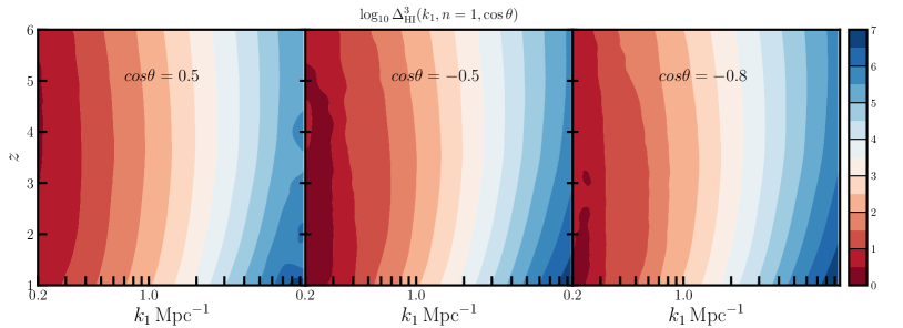
Figure 2: This shows the joint $k_{1}$ and $z$ dependence of $\Delta^{3}_{{\rm HI}\,}(k_{1},n,{\cos\theta}\,)$ for the isosceles triangles (i.e. $n=1$) at three different values of ${\cos\theta}\,$.

Figure 2 shows the joint $k_{1}$ and $z$ dependence of $\Delta^{3}_{{\rm HI}\,}(k_{1},n,{\cos\theta}\,)$ for isosceles triangles (i.e. $n=1$) at three different values of ${\cos\theta}\,$. We first discuss the central panel which considers ${\cos\theta}\,=-0.5$ that corresponds to equilateral triangle. The equilateral triangle is a special case where the three Fourier modes that appear in the bispectrum (Equation 3) have equal magnitude $(k_{1}=k_{2}=k_{3})$. Considering any fixed redshift $z$, we see that $\Delta^{3}_{{\rm HI}\,}(k_{1},n,{\cos\theta}\,)$ increases monotonically with increasing $k_{1}$. We notice that the $\Delta^{3}_{{\rm HI}\,}(k_{1},n,{\cos\theta}\,)$ contours are nearly vertical in the range $k_{1}<0.4\,{{\rm Mpc}^{-1}}$ which implies $\Delta^{3}_{{\rm HI}\,}(k_{1},n,{\cos\theta}\,)$ does not vary much with redshift in this $k$ range. However, the $\Delta^{3}_{{\rm HI}\,}(k_{1},n,{\cos\theta}\,)$ contours are inclined and also curved for $k_{1}>0.4\,{{\rm Mpc}^{-1}}$ indicating a significant variation with $z$. Considering a fixed value of $k_{1}$ in the range $k_{1}>0.4\,{{\rm Mpc}^{-1}}$ we see that, $\Delta^{3}_{{\rm HI}\,}(k_{1},n,{\cos\theta}\,)$ first decreases with increasing $z$, then becomes minimum at $z\sim 3.5$ and increases again at $z>4$. The left-hand and right-hand panels show results for ${\cos\theta}\,=0.5$ and ${\cos\theta}\,=-0.8$ which corresponds to obtuse and acute triangles respectively. We see that for both the obtuse and acute triangles the behaviour of $\Delta^{3}_{{\rm HI}\,}(k_{1},n,{\cos\theta}\,)$ is similar to that of the equilateral triangle. These results are also very similar if we consider $n=2$ and $n=5$ and we have not shown these here.

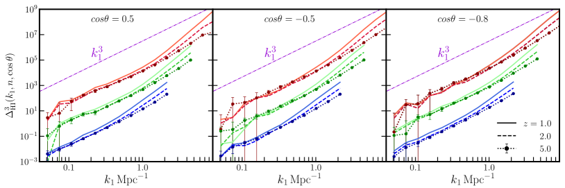
Figure 3: This shows $\Delta^{3}_{{\rm HI}\,}(k_{1},n,{\cos\theta}\,)$ as a function of $k_{1}$ for the same three values of ${\cos\theta}\,$ ($0.5,-0.5,-0.8$) as those considered in Figure 2. In each panel, the results for the $n=1,2$ and $5$ triangles are plotted together. The results for the different $n$ values overlap for almost the entire $k_{1}$ range, and we have multiplied the results for $n=1$ and $2$ with $100$ and $10$ respectively in order to show them clearly. We also show the power law $\sim k_{1}^{3}$ for convenience.

The three panels of Figure 3 show $\Delta^{3}_{{\rm HI}\,}(k_{1},n,{\cos\theta}\,)$ as a function of $k_{1}$ for the same three values of ${\cos\theta}\,$ ($0.5,-0.5,-0.8$) as those considered in Figure 2. In each panel, the results for the $n=1,2$ and $5$ triangles are plotted together. The results for the different $n$ values overlap for almost the entire $k_{1}$ range, and we have multiplied the results for $n=1$ and $2$ with $100$ and $10$ respectively in order to show them clearly. In all cases the amplitude and $k_{1}$ dependence of $\Delta^{3}_{{\rm HI}\,}(k_{1},n,{\cos\theta}\,)$ is almost constant with redshift at $z\geq 3$, and consequently we show the results at only three redshifts $z=1,2$ and $5$. Considering all the results together, we see that $\Delta^{3}_{{\rm HI}\,}(k_{1},n,{\cos\theta}\,)$ exhibits a power law behaviour $\Delta^{3}_{{\rm HI}\,}\sim k_{1}^{\alpha}$ for $k_{1}<1\,{{\rm Mpc}^{-1}}$ with $\alpha\approx 3$ which is nearly independent of redshift, only the amplitude of $\Delta^{3}_{{\rm HI}\,}(k_{1},n,{\cos\theta}\,)$ changes with redshift. However this power law does not hold at small $k_{1}$ ($<0.1\,{{\rm Mpc}^{-1}}$) where the cosmic variance dominates. We also see that $\Delta^{3}_{{\rm HI}\,}(k_{1},n,{\cos\theta}\,)$ is steeper than $k_{1}^{3}$ at large $k_{1}$ ($>1\,{{\rm Mpc}^{-1}}$) where the non-linear effects are important, and this steepening increases at lower redshifts. We also note that for $n=5$ the steeping sets in at a smaller value of $k_{1}$ as compared to $n=1$. This is consistent with the notion that the steepening arises from the small-scale non-linear effects which are expected to be more pronounced for $n=5$ ($k_{2}=5k_{1}$) as compared to $n=1$.

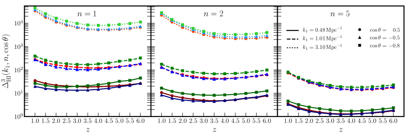
Figure 4: This shows the variation of $\Delta^{3}_{{\rm HI}\,}(k_{1},n,{\cos\theta}\,)$ with redshift at fixed values of $k_{1}$ and ${\cos\theta}\,$. We consider three representative $k_{1}$ values $(0.48,1.01,3.10)\,{{\rm Mpc}^{-1}}$, and ${\cos\theta}\,=(0.5,-0.5,-0.8)$ same as in the earlier figures. The left-hand, central and right-hand panels show results for $n=1,2$ and $5~{}$ respectively. Note that for $n=5$ we do not have results at $k_{1}=3.10\,{{\rm Mpc}^{-1}}$ as the corresponding $k_{2}(=5k_{1})$ is beyond the range of our simulations.

Figure 4 shows the variation of $\Delta^{3}_{{\rm HI}\,}(k_{1},n,{\cos\theta}\,)$ with redshift at fixed values of $k_{1}$ and ${\cos\theta}\,$. We consider three representative $k_{1}$ values $(0.48,1.01,3.10)\,{{\rm Mpc}^{-1}}$ which correspond to progressively increasing non-linear effects, and ${\cos\theta}\,=(0.5,-0.5,-0.8)$ same as in the earlier figures. The left-hand, central and right-hand panels show results for $n=1,2$ and $5~{}$ respectively. Note that for $n=5$ we do not have results at $k_{1}=3.10\,{{\rm Mpc}^{-1}}$ as the corresponding $k_{2}(=5k_{1})$ is beyond the range of our simulations. We see that the value of $\Delta^{3}_{{\rm HI}\,}(k_{1},n,{\cos\theta}\,)$ increases significantly if $k_{1}$ increases, decreases to some extent if $n$ is increased, and shows a relatively smaller variation with ${\cos\theta}\,$. Considering the overall $z$ dependence, we see that with decreasing $z$ the value of $\Delta^{3}_{{\rm HI}\,}(k_{1},n,{\cos\theta}\,)$ initially decreases, shows a minima at $z\sim 3.5$ and then increases at lower redshifts. This redshift evolution is relatively weak at the smallest $k_{1}$ which is weakly non-linear at $z\leq 2$ (see Figure 2 of Paper I). The redshift evolution is most pronounced at the largest $k_{1}$ which is strongly non-linear at $z\leq 3$ where $\Delta^{3}_{{\rm HI}\,}(k_{1},n,{\cos\theta}\,)$ shows a noticeable increase with decreasing $z$. We also find a more pronounced redshift evolution for the larger $n$ where the non-linear effects are expected to be stronger. We note that the bispectrum of the underlying matter distribution is expected to increase monotonically as $z$ decreases. In contrast, we see that the HI bispectrum first declines and then increases as $z$ decreases. This, as we shall see later, can be understood in terms of the redshift evolution of the HI bias.

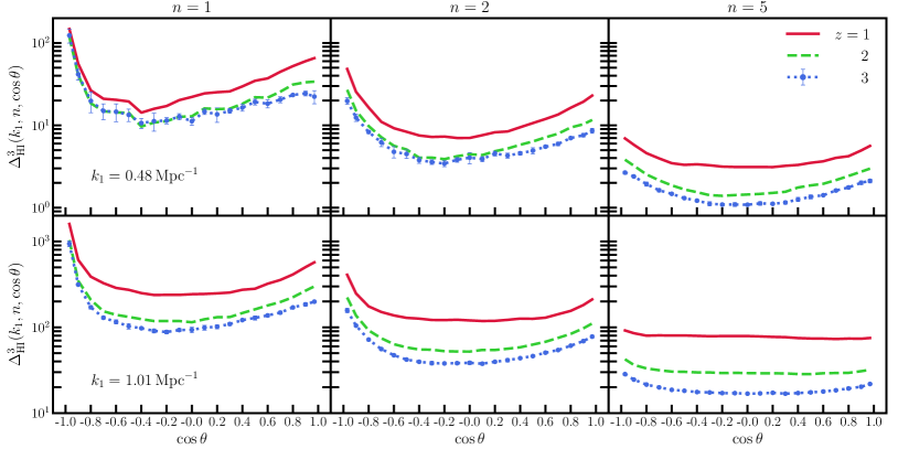
Figure 5: This shows $\Delta^{3}_{{\rm HI}\,}(k_{1},n,{\cos\theta}\,)$ as a function of ${\cos\theta}\,$ at three different redshifts $z=1,2$ and $3$. The top and bottom rows show results at $k_{1}=0.48$ and $1.01\,{{\rm Mpc}^{-1}}$ respectively, while the left, central and right columns show results for $n=1,2$ and $5$ respectively. The $1-\sigma$ spread estimated from five statistically independent realizations of the simulations is shown for results at $z=3$.

Figure 5 shows $\Delta^{3}_{{\rm HI}\,}(k_{1},n,{\cos\theta}\,)$ as a function of ${\cos\theta}\,$ at three different redshifts $z=1,2$ and $3$, we have similar results at higher redshifts where the curves overlap and we have not shown these here. The top and bottom rows show results at $k_{1}=0.48$ and $1.01\,{{\rm Mpc}^{-1}}$ respectively, while the left, central and right columns show results for $n=1,2$ and $5$ respectively. Considering all the panels together, in nearly all cases we have a “U" shaped curve relating $\Delta^{3}_{{\rm HI}\,}(k_{1},n,{\cos\theta}\,)$ to ${\cos\theta}\,$. The minima appears to be independent of $k_{1}$ and $z$, and shifts from ${\cos\theta}\,\approx-0.5$ to $-0.2$ and $0$ for $n=1,2$ and $5$. The “U" shaped ${\cos\theta}\,$ dependence is well pronounced for $n=1$ and $2$ at the higher redshifts where the $\mathbf{k}$ modes involved are weakly non-linear. However, the “U" is rather broad and sometimes nearly flat in many cases, particularly at low $z$ $(=1)$ or if either of $k_{1}$ or $n$ is increased and the $\mathbf{k}$ modes involved are strongly non-linear. It is difficult to reliably estimate the minima in these cases.

4 Modelling the HI Bispectrum

We assume that the HI traces the dark matter with a possible bias. Here we retain terms upto the quadratic order in the relation between HI density contrast $\delta_{{\rm HI}\,}$ and the dark matter density contrast $\delta$

$$\delta_{{\rm HI}\,}=b_{1}\delta+\frac{b_{2}}{2}\delta^{2}\,,$$ (7)

where $b_{1}$ and $b_{2}$ are the linear and quadratic bias parameters respectively. The linear bias $b_{1}$ can be calculated using the relation

$$P_{{\rm HI}\,}=b_{1}^{2}P\,,$$ (8)

where $P_{{\rm HI}\,}$ and $P$ are respectively the HI and the dark matter power spectra. Paper I presents a detailed analysis of the linear HI bias allowing for the possibility that $\tilde{b}_{1}(k)$, defined in Fourier space, is both complex and $k$ dependent. The analysis however shows that it is adequate to assume a real scale-independent bias at small $k$. The quadratic bias $b_{2}$ introduces non-linearity in the relation between $\delta_{{\rm HI}\,}$ and $\delta$. Here $b_{1}$ and $b_{2}$ both have been assumed to be real scale-independent quantities which vary only with redshift.

Considering second order (Fry, 1984) perturbation theory, Matarrese et al. (1997) and Scoccimarro (2000) have calculated the bispectrum for a biased tracer of the underlying dark matter distribution. Applying this to the HI field (Equation 7) we have

$$B_{{\rm HI}\,}({\bf k_{1}},{\bf k_{2}},{\bf k_{3}})=b_{1}^{3}\left[2F({\bf k_{1}},{\bf k_{2}})P(k_{1})P(k_{2})+\text{cyc.}\right]\\ +b_{1}^{2}b_{2}\left[P(k_{1})P(k_{2})+\text{cyc.}\right]\,,$$ (9)

where

$$F({\bf k_{1}},{\bf k_{2}})=\left(\frac{1+\kappa}{2}\right)+\left(\frac{{\bf k_{1}}.{\bf k_{2}}}{2k_{1}k_{2}}\right)\left(\frac{k_{1}}{k_{2}}+\frac{k_{2}}{k_{1}}\right)\\ +\left(\frac{1-\kappa}{2}\right)\left(\frac{{\bf k_{1}}.{\bf k_{2}}}{k_{1}k_{2}}\right)^{2}\,,$$ (10)

with $\kappa=\frac{3}{7}\Omega_{m}^{-\frac{1}{143}}$ for the $\Lambda CDM$ cosmology. Here we find that it is convenient to model the HI bispectrum $B_{{\rm HI}\,}({\bf k_{1}},{\bf k_{2}},{\bf k_{3}})$ in terms of the HI power spectrum $P_{{\rm HI}\,}(k)$ using Equation 8 whereby we obtain

$$B_{{\rm HI}\,}({\bf k_{1}},{\bf k_{2}},{\bf k_{3}})=\frac{1}{b_{1}}\left[2F({\bf k_{1}},{\bf k_{2}})P_{{\rm HI}\,}(k_{1})P_{{\rm HI}\,}(k_{2})+\text{cyc.}\right]\\ +\frac{b_{2}}{b_{1}^{2}}\left[P_{{\rm HI}\,}(k_{1})P_{{\rm HI}\,}(k_{2})+\text{cyc.}\right]\,.$$ (11)

We have used Equation 11 to model the HI bispectrum $B_{{\rm HI}\,}({\bf k_{1}},{\bf k_{2}},{\bf k_{3}})$. The HI power spectrum $P_{{\rm HI}\,}(k)$ is known from simulations and this has been studied in Paper I. The model therefore has only two free parameters, namely the two HI bias parameters $b_{1}$ and $b_{2}$. The second term in the r.h.s. of Equation 11 depends only on the magnitude of the three modes ${\bf k_{1}},{\bf k_{2}}$ and ${\bf k_{3}}$ whereas the first term also depends on the shape of the triangle through $F({\bf k_{1}},{\bf k_{2}})$. This feature allows us to separately determine $b_{1}$ and $b_{2}$ by fitting the model (Equation 11) to the HI bispectrum obtained from the simulations. We note that the model used here is entirely based on second order perturbation theory which is expected to hold only in the weakly non-linear regime. Many of the modes considered here are however in the strongly non-linear regime where we do not expect the model to provide an adequate description of the HI bispectrum. We therefore first need to establish the range of Fourier modes $({\bf k_{1}},{\bf k_{2}},{\bf k_{3}})$ where the model (Equation 11) provides an adequate description of the HI bispectrum obtained from the simulations.

$z$	$n$	$k_{1}\,{{\rm Mpc}^{-1}}$
$1$	$1$	$0.33,0.48$
	$2$	$0.33$
	$5$	$0.16$
$1.5-2$	$1$	$0.33,0.48$
	$2$	$0.33,0.48$
	$5$	$0.16$
$2.5-4.5$	$1$	$0.33,0.48,0.70$
	$2$	$0.33,0.48,0.70$
	$5$	$0.16$
$5.0-6.0$	$1$	$0.33,0.48,0.70$
	$2$	$0.33$
	$5$	$0.16$

Table 1: This presents the $k_{1}$ and $n$ values that we have used for fitting the HI bispectrum at different redshifts.

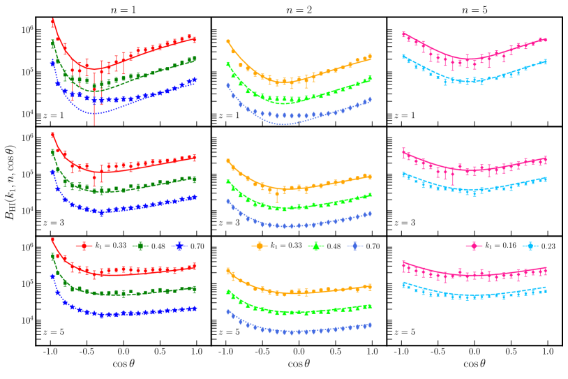
Figure 6: This shows the best fit prediction of our model (Equation 11) for the HI bispectrum along with the simulated values for various triangle configurations. The top, middle and bottom rows show results at $z=1,3$ and $5$, while the left, central and right columns show results for $n=1,2$ and $5$. For each $n$ value, results for different $k_{1}$ (in unit of $\,{{\rm Mpc}^{-1}}$) are shown with different symbols and line styles.

We have performed a $\chi^{2}$ minimization with respect to $b_{1}$ and $b_{2}$ in order to determine the parameter values for which the model (Equation 11) best fits $B_{{\rm HI}\,}(k_{1},n,{\cos\theta}\,)$ obtained from the simulations. Note that we have used $P_{{\rm HI}\,}(k)$ obtained in Paper I for the fits. As mentioned earlier, the bias parameters $b_{1}$ and $b_{2}$ are assumed to evolve with redshift and we have separately carried out the fitting at each redshift. We have initially attempted to fit $B_{{\rm HI}\,}(k_{1},n,{\cos\theta}\,)$ using the entire $(k_{1},n,{\cos\theta}\,)$ range available in the simulations, we however find that the best fit reduced $\chi^{2}$ is rather large indicating a poor fit. While our model is expected to perform well at small $k$ (large scales), we find that the sample variance is quite large for the first few $k_{1}$ bins and hence we do not use these for the subsequent fitting. We also do not expect our model to work at large $k$ which are strongly non-linear, and we find that our model predictions deviate significantly from the simulated values. At each redshift, for the various combinations of $k_{1}$ and $n$ we have individually considered $B_{{\rm HI}\,}(k_{1},n,{\cos\theta}\,)$ as a function of ${\cos\theta}\,$, some of these are shown in Figure 6. We find a good fit with reduced $\chi^{2}$ of the order of unity provided we restrict the $k_{1},\,n$ values to the range shown in Table 1, we however consider the full range $-1<{\cos\theta}\,<1$ throughout. Note that the $k_{1},\,n$ range varies with $z$. The non-linear effects increase at lower redshifts, and the combinations with larger $k_{1}$ and $n$ values are progressively dropped at lower redshifts.

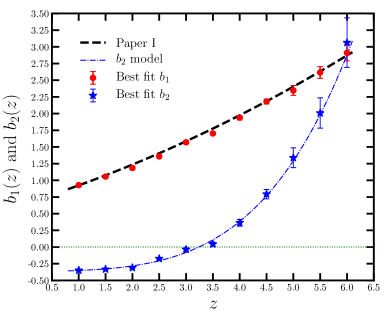
Figure 7: This shows the best-fitting values of the bias parameters $b_{1}$ (red circles) and $b_{2}$ (blue stars) at different redshifts. Error bars show the $1-\sigma$ fitting uncertainties for the respective quantities. The black dashed line shows $b_{1}$ calculated using Equation 12 whereas the blue line shows the prediction of Equation 13 for $b_{2}$.

Figure 6 shows the best fit prediction of our model (Equation 11) for the HI bispectrum along with the simulated values for various triangle configurations. Considering the $n=1$ and $2$ triangles, we see that the model provides a reasonably good fit to all the simulated values shown here except $k_{1}=0.70\,{{\rm Mpc}^{-1}}$ at $z=1$ where the model underpredicts the bispectrum. Considering the $n=5$ triangles, we see that the model provides a reasonably good fit to the simulations for $k_{1}=0.16\,{{\rm Mpc}^{-1}}$ at all redshifts, the model overpredicts the bispectrum at other $k_{1}$ values.

Figure 7 shows the best-fitting values of the two bias parameters $b_{1}$ and $b_{2}$ at different redshifts. We see that the best fit linear HI bias $b_{1}$ falls almost linearly with decreasing $z$. In Paper I we have determined $b_{1}$ using the ratio of the power spectra (Equation 8) allowing for both the scale $(k)$ dependence and redshift evolution, and we have modelled the joint $k$ and $z$ dependence of $b_{1}(k,z)$ using a polynomial which is quartic in $k$ and quadratic in $z$ (Equation A1 of Paper I). In the present work we consider the $k\rightarrow 0$ limit of $b_{1}(k,z)$ obtained in Paper I to predict the scale-independent component of $b_{1}$ (see Figures 4 and 5 of Paper I) whose $z$ dependence can be modelled using the polynomial

$$b_{1}(z)=b_{10}+b_{11}z+b_{12}z^{2}\,,$$ (12)

where the coefficients have values $(b_{10},b_{11},b_{12})=(0.653,0.252,0.0196)$. We have plotted the predictions of Equation 12 in Figure 7 (black dashed line). We find that across the entire $z$ range the best-fitting values of $b_{1}$ obtained by modelling the HI bispectrum are in good agreement with the predictions of Equation 12 obtained in Paper I by modelling the HI power spectrum. Considering the quadratic HI bias $b_{2}$ in Figure 7 we see that it starts from a value $\approx 3.1$ at $z=6$ and declines rapidly with decreasing $z$, crosses zero at $z\sim 3$ and then flattens out at a negative value $\approx-0.36$ at $z<2$. We find that the $z$ dependence of $b_{2}$ can be very well modelled using a quartic polynomial in $z$ containing only even terms,

$$b_{2}(z)=b_{20}+b_{22}z^{2}+b_{24}z^{4}\,,$$ (13)

with the fitting parameters $(b_{20},b_{22},b_{24})=(-0.365,0.0121,0.00217)$.

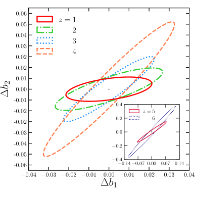
Figure 8: This shows $1-\sigma$ error covariance ellipses obtained from the joint fitting of the two bias parameters $b_{1}$ and $b_{2}$ at different redshifts. The error covariance ellipses at $z=5$ and $6$ are shown in the inset.

Figure 8 shows $1-\sigma$ error covariance ellipses obtained from the joint fitting of the two bias parameters $b_{1}$ and $b_{2}$ at different redshifts. The signal to noise ratio of the estimated bispectrum increases with decreasing redshift. We see that the errors in the two bias parameters show the same behaviour i.e. the errors decrease with decreasing redshift. The correlation between the errors, as inferred from the tilt of the ellipses, also decreases with decreasing $z$.

5 Summary and Discussion

We have determined the bispectrum of the post-reionization HI 21-cm signal using simulations. The simulations start from Gaussian initial conditions and the bispectrum emerges from the non-linear gravitational clustering and the non-linear bias of the HI distribution. We find that the dimensionless HI bispectrum $\Delta^{3}_{{\rm HI}\,}(k_{1},n,{\cos\theta}\,)$ increases monotonically with $k_{1}$ (Figure 2) and it shows an approximate power law dependence on the size of the triangle $\Delta^{3}_{{\rm HI}\,}\sim k_{1}^{3}$ (Figure 3) almost independent of redshift and the shape of the triangle. This scaling is found to be largely restricted to the weakly non-linear regime ($k_{1}<1\,{{\rm Mpc}^{-1}}$), and the $k_{1}$ dependence is found to steepen at larger $k_{1}$ and larger $n$ values where the modes involved are in the strongly non-linear regime. Considering the $z$ dependence, we find that the amplitude of $\Delta^{3}_{{\rm HI}\,}(k_{1},n,{\cos\theta}\,)$ does not evolve significantly with $z$ at $k_{1}<0.4\,{{\rm Mpc}^{-1}}$ (Figure 2). We find that $\Delta^{3}_{{\rm HI}\,}(k_{1},n,{\cos\theta}\,)$ shows a weak $z$ evolution at $k_{1}>0.4\,{{\rm Mpc}^{-1}}$, its amplitude initially decreases with decreasing $z$ reaching a minima at $z\sim 3.5$ and then increases at lower $z$ (Figure 4). The increase at low $z$ is particularly more pronounced at large $k_{1}$ and $n$ where the modes involved are strongly non-linear. We see (Figures 5 and 6) that $\Delta^{3}_{{\rm HI}\,}(k_{1},n,{\cos\theta}\,)$ has a “U" shaped ${\cos\theta}\,$ dependence. The “U" shape is well pronounced when the modes involved are in the weakly non-linear regime. However, this “U" shape is flattened out at large $k_{1}$ and $n$ where the modes involved are in the strongly non-linear regime.

Here we have modelled the HI bispectrum using Equation 11 which is based on second order perturbation theory (Scoccimarro, 2000). The model expresses the HI bispectrum in terms of the HI power spectrum and $b_{1}$ and $b_{2}$ which are respectively the linear and quadratic HI bias parameters. We have used the HI power spectrum from Paper I, and the model then has only two unknown parameters $b_{1}$ and $b_{2}$ which are assumed to evolve with redshift. We find that the model provides a good fit to the HI bispectrum obtained from the simulations provided we excluded the triangles where the modes are in the strongly non-linear regime. The linear bias $b_{1}$ is found to be decreasing nearly linearly with $z$, and the values are in good agreement with the large scale ($k_{1}\rightarrow 0$) linear bias estimated in Paper I by directly modelling the simulated HI power spectrum. On the other hand, the best-fitting values of the quadratic bias $b_{2}$ falls sharply with decreasing $z$, becomes zero at $z\sim 3$ and attains a nearly constant value $b_{2}\approx-0.36$ at $z<2$. We have provided polynomial fitting formulae for the $z$ dependence of both $b_{1}$ and $b_{2}$. We note that $b_{2}\approx 0$ at $z\sim 3$ which implies that the HI is linearly biased with respect to the underlying dark matter at this redshift.

The post-reionization HI 21-cm signal is a potential tool for precision cosmology. Measurements of the redshift-space 21-cm power spectrum (discussed in Paper II and III) can be used to estimate the redshift distortion parameter $\beta=f(\Omega_{m})/b_{1}$. As discussed here, measurements of the 21-cm bispectrum can be used to estimate the HI bias parameters $b_{1}$ and $b_{2}$. These can be combined to estimate the cosmological growth rate $f(\Omega_{m})$ which is not only a sensitive probe of cosmology but can also be used to distinguish between various theories of gravitation. It is also possible to use the measured 21-cm bispectrum to constrain primordial non-Gaussianity provided one has a precise model for the 21-cm bispectrum expected from Gaussian initial conditions. We plan to investigate these issues in future work. Further, the entire analysis here does not take into account redshift-space distortion due to peculiar velocities. We plan to incorporate this in future work.

References

- Ali et al. (2006) Ali S. S. S., Bharadwaj S., Pandey S. K., 2006, MNRAS, 366, 213
- Bagla et al. (2010) Bagla J. S., Khandai N., Datta K. K., 2010, MNRAS, 407, 567
- Ballardini et al. (2019) Ballardini M., Matthewson W. L., Maartens R., 2019, arXiv e-prints, p. arXiv:1906.04730
- Bandura et al. (2014) Bandura K., et al., 2014, in Society of Photo-Optical Instrumentation Engineers (SPIE) Conference Series. p. 22 (arXiv:1406.2288), doi:10.1117/12.2054950
- Barnes & Haehnelt (2014) Barnes L. A., Haehnelt M. G., 2014, MNRAS, 440, 2313
- Battye et al. (2012) Battye R. A., et al., 2012, ArXiv e-prints: 1209.1041,
- Bean et al. (1983) Bean A. J., Ellis R. S., Shanks T., Efstathiou G., Peterson B. A., 1983, MNRAS, 205, 605
- Bharadwaj (1994) Bharadwaj S., 1994, ApJ, 428, 419
- Bharadwaj & Pandey (2003) Bharadwaj S., Pandey S. K., 2003, Journal of Astrophysics and Astronomy, 24, 23
- Bharadwaj & Pandey (2005) Bharadwaj S., Pandey S. K., 2005, MNRAS, 358, 968
- Bharadwaj & Sethi (2001) Bharadwaj S., Sethi S. K., 2001, Journal of Astrophysics and Astronomy, 22, 293
- Bharadwaj & Srikant (2004) Bharadwaj S., Srikant P. S., 2004, Journal of Astrophysics and Astronomy, 25, 67
- Bharadwaj et al. (2001) Bharadwaj S., Nath B. B., Sethi S. K., 2001, Journal of Astrophysics and Astronomy, 22, 21
- Bharadwaj et al. (2009) Bharadwaj S., Sethi S. K., Saini T. D., 2009, Phys. Rev. D, 79, 083538
- Bigot-Sazy et al. (2016) Bigot-Sazy M.-A., et al., 2016, in Qain L., Li D., eds, Astronomical Society of the Pacific Conference Series Vol. 502, Frontiers in Radio Astronomy and FAST Early Sciences Symposium 2015. p. 41 (arXiv:1511.03006)
- Bull et al. (2015) Bull P., Ferreira P. G., Patel P., Santos M. G., 2015, ApJ, 803, 21
- Cappi et al. (2015) Cappi A., et al., 2015, A&A, 579, A70
- Carucci et al. (2017) Carucci I. P., Villaescusa-Navarro F., Viel M., 2017, J. Cosmology Astropart. Phys., 4, 001
- Castorina & Villaescusa-Navarro (2017) Castorina E., Villaescusa-Navarro F., 2017, MNRAS, 471, 1788
- Chang & GBT-HIM Team (2016) Chang T.-C., GBT-HIM Team 2016, in American Astronomical Society Meeting Abstracts. p. 426.01
- Chang et al. (2008) Chang T.-C., Pen U.-L., Peterson J. B., McDonald P., 2008, Physical Review Letters, 100, 091303
- Chang et al. (2010) Chang T.-C., Pen U.-L., Bandura K., Peterson J. B., 2010, Nature, 466, 463
- Chen et al. (2016) Chen Z. P., Wang R. L., Peterson J., Chen X. L., Zhang J. Y., Shi H. L., 2016, in Ground-based and Airborne Telescopes VI. p. 99065W, doi:10.1117/12.2232570
- Chongchitnan (2013) Chongchitnan S., 2013, J. Cosmology Astropart. Phys., 3, 037
- Choudhuri (2017) Choudhuri S., 2017, preprint, (arXiv:1708.04277)
- Davé et al. (2013) Davé R., Katz N., Oppenheimer B. D., Kollmeier J. A., Weinberg D. H., 2013, MNRAS, 434, 2645
- Davis et al. (1985) Davis M., Efstathiou G., Frenk C. S., White S. D. M., 1985, ApJ, 292, 371
- Efstathiou & Jedrzejewski (1984) Efstathiou G., Jedrzejewski R. I., 1984, Advances in Space Research, 3, 379
- Feldman et al. (2001) Feldman H. A., Frieman J. A., Fry J. N., Scoccimarro R., 2001, Physical Review Letters, 86, 1434
- Fry (1984) Fry J. N., 1984, ApJ, 279, 499
- Fry (1994) Fry J. N., 1994, Physical Review Letters, 73, 215
- Fry & Seldner (1982) Fry J. N., Seldner M., 1982, ApJ, 259, 474
- Gaztanaga & Frieman (1994) Gaztanaga E., Frieman J. A., 1994, ApJ, 437, L13
- Gil-Marín et al. (2015) Gil-Marín H., Noreña J., Verde L., Percival W. J., Wagner C., Manera M., Schneider D. P., 2015, MNRAS, 451, 539
- Groth & Peebles (1977) Groth E. J., Peebles P. J. E., 1977, ApJ, 217, 385
- Guha Sarkar (2010) Guha Sarkar T., 2010, J. Cosmology Astropart. Phys., 2, 002
- Guha Sarkar & Bharadwaj (2013) Guha Sarkar T., Bharadwaj S., 2013, J. Cosmology Astropart. Phys., 8, 023
- Guha Sarkar & Hazra (2013) Guha Sarkar T., Hazra D. K., 2013, J. Cosmology Astropart. Phys., 4, 002
- Guha Sarkar et al. (2009) Guha Sarkar T., Datta K. K., Bharadwaj S., 2009, J. Cosmology Astropart. Phys., 8, 019
- Guha Sarkar et al. (2012) Guha Sarkar T., Mitra S., Majumdar S., Choudhury T. R., 2012, MNRAS, 421, 3570
- Guo et al. (2015) Guo H., et al., 2015, MNRAS, 449, L95
- Gupta (2017) Gupta Y., 2017, in Current Science. pp 707–714, doi:10.18520/cs/v113/i04/707-714
- Hale-Sutton et al. (1989) Hale-Sutton D., Fong R., Metcalfe N., Shanks T., 1989, MNRAS, 237, 569
- Hoffmann et al. (2018) Hoffmann K., Mao Y., Xu J., Mo H., Wandelt B. D., 2018, arXiv e-prints,
- Jackson (1972) Jackson J. C., 1972, MNRAS, 156, 1P
- Johnston et al. (2008) Johnston S., et al., 2008, Experimental Astronomy, 22, 151
- Kaiser (1987) Kaiser N., 1987, MNRAS, 227, 1
- Khandai et al. (2011) Khandai N., Sethi S. K., Di Matteo T., Croft R. A. C., Springel V., Jana A., Gardner J. P., 2011, MNRAS, 415, 2580
- Kim et al. (2017) Kim H.-S., Wyithe J. S. B., Baugh C. M., Lagos C. d. P., Power C., Park J., 2017, MNRAS, 465, 111
- Kovetz et al. (2017) Kovetz E. D., et al., 2017, preprint, (arXiv:1709.09066)
- Kuhn et al. (2019) Kuhn E., Saliwanchik B., Newburgh L., 2019, in American Astronomical Society Meeting Abstracts #233. p. 146.19
- Loeb & Wyithe (2008) Loeb A., Wyithe J. S. B., 2008, Physical Review Letters, 100, 161301
- Majumdar et al. (2018) Majumdar S., Pritchard J. R., Mondal R., Watkinson C. A., Bharadwaj S., Mellema G., 2018, MNRAS, 476, 4007
- Masui et al. (2010) Masui K. W., McDonald P., Pen U.-L., 2010, Phys. Rev. D, 81, 103527
- Masui et al. (2013) Masui K. W., et al., 2013, ApJ, 763, L20
- Matarrese et al. (1997) Matarrese S., Verde L., Heavens A. F., 1997, MNRAS, 290, 651
- Moresco et al. (2017) Moresco M., et al., 2017, A&A, 604, A133
- Nishimichi et al. (2007) Nishimichi T., Kayo I., Hikage C., Yahata K., Taruya A., Jing Y. P., Sheth R. K., Suto Y., 2007, PASJ, 59, 93
- Obuljen et al. (2018) Obuljen A., Castorina E., Villaescusa-Navarro F., Viel M., 2018, J. Cosmology Astropart. Phys., 5, 004
- Padmanabhan & Kulkarni (2017) Padmanabhan H., Kulkarni G., 2017, MNRAS, 470, 340
- Padmanabhan & Refregier (2017) Padmanabhan H., Refregier A., 2017, MNRAS, 464, 4008
- Padmanabhan et al. (2017) Padmanabhan H., Refregier A., Amara A., 2017, MNRAS, 469, 2323
- Padmanabhan et al. (2019) Padmanabhan H., Refregier A., Amara A., 2019, MNRAS,
- Peebles (1980) Peebles P. J. E., 1980, The large-scale structure of the universe
- Peebles & Groth (1976) Peebles P. J. E., Groth E. J., 1976, A&A, 53, 131
- Pen et al. (2009) Pen U.-L., Staveley-Smith L., Peterson J. B., Chang T.-C., 2009, MNRAS, 394, L6
- Pénin et al. (2018) Pénin A., Umeh O., Santos M. G., 2018, MNRAS, 473, 4297
- Pillepich et al. (2007) Pillepich A., Porciani C., Matarrese S., 2007, ApJ, 662, 1
- Planck Collaboration et al. (2016a) Planck Collaboration et al., 2016a, A&A, 594, A13
- Planck Collaboration et al. (2016b) Planck Collaboration et al., 2016b, A&A, 594, A17
- Planck Collaboration et al. (2019) Planck Collaboration et al., 2019, arXiv e-prints, p. arXiv:1905.05697
- Santos et al. (2015) Santos M., et al., 2015, Advancing Astrophysics with the Square Kilometre Array (AASKA14), p. 19
- Sarkar & Bharadwaj (2018) Sarkar D., Bharadwaj S., 2018, MNRAS, 476, 96
- Sarkar & Bharadwaj (2019) Sarkar D., Bharadwaj S., 2019, MNRAS,
- Sarkar et al. (2016) Sarkar D., Bharadwaj S., Anathpindika S., 2016, MNRAS, 460, 4310
- Sarkar et al. (2017) Sarkar A. K., Bharadwaj S., Ali S. S., 2017, Journal of Astrophysics and Astronomy, 38, 14
- Sarkar et al. (2018) Sarkar A. K., Bharadwaj S., Guha Sarkar T., 2018, J. Cosmology Astropart. Phys., 5, 051
- Schmit et al. (2019) Schmit C. J., Heavens A. F., Pritchard J. R., 2019, MNRAS, 483, 4259
- Scoccimarro (2000) Scoccimarro R., 2000, ApJ, 544, 597
- Scoccimarro et al. (1998) Scoccimarro R., Colombi S., Fry J. N., Frieman J. A., Hivon E., Melott A., 1998, ApJ, 496, 586
- Scoccimarro et al. (2001) Scoccimarro R., Feldman H. A., Fry J. N., Frieman J. A., 2001, ApJ, 546, 652
- Seo et al. (2010) Seo H.-J., Dodelson S., Marriner J., Mcginnis D., Stebbins A., Stoughton C., Vallinotto A., 2010, ApJ, 721, 164
- Serra et al. (2012) Serra P., et al., 2012, MNRAS, 422, 1835
- Shimabukuro et al. (2016) Shimabukuro H., Yoshiura S., Takahashi K., Yokoyama S., Ichiki K., 2016, MNRAS, 458, 3003
- Shimabukuro et al. (2017) Shimabukuro H., Yoshiura S., Takahashi K., Yokoyama S., Ichiki K., 2017, MNRAS, 468, 1542
- Slepian et al. (2017) Slepian Z., et al., 2017, MNRAS, 468, 1070
- Subrahmanya et al. (2017) Subrahmanya C. R., Manoharan P. K., Chengalur J. N., 2017, Journal of Astrophysics and Astronomy, 38, 10
- Switzer et al. (2013) Switzer E. R., et al., 2013, MNRAS, 434, L46
- Umeh (2017) Umeh O., 2017, J. Cosmology Astropart. Phys., 6, 005
- Umeh et al. (2016) Umeh O., Maartens R., Santos M., 2016, J. Cosmology Astropart. Phys., 3, 061
- Verde et al. (1998) Verde L., Heavens A. F., Matarrese S., Moscardini L., 1998, MNRAS, 300, 747
- Verde et al. (2002) Verde L., et al., 2002, MNRAS, 335, 432
- Villaescusa-Navarro et al. (2014) Villaescusa-Navarro F., Viel M., Datta K. K., Choudhury T. R., 2014, J. Cosmology Astropart. Phys., 9, 50
- Villaescusa-Navarro et al. (2015) Villaescusa-Navarro F., Viel M., Alonso D., Datta K. K., Bull P., Santos M. G., 2015, J. Cosmology Astropart. Phys., 3, 034
- Villaescusa-Navarro et al. (2016) Villaescusa-Navarro F., et al., 2016, MNRAS, 456, 3553
- Watkinson et al. (2017) Watkinson C. A., Majumdar S., Pritchard J. R., Mondal R., 2017, MNRAS, 472, 2436
- Wyithe & Loeb (2008) Wyithe J. S. B., Loeb A., 2008, MNRAS, 383, 606
- Wyithe & Loeb (2009) Wyithe J. S. B., Loeb A., 2009, MNRAS, 397, 1926
- Wyithe et al. (2008) Wyithe J. S. B., Loeb A., Geil P. M., 2008, MNRAS, 383, 1195
- Yoshiura et al. (2015) Yoshiura S., Shimabukuro H., Takahashi K., Momose R., Nakanishi H., Imai H., 2015, MNRAS, 451, 266