OPTION PRICING IN FRACTIONAL HESTON-TYPE MODEL

Abstract.

In this paper, we consider option pricing in a framework of the fractional Heston-type model with $H>1/2$. As it is impossible to obtain an explicit formula for the expectation $\mathbb{E}f(S_{T})$ in this case, where $S_{T}$ is the asset price at maturity time and $f$ is a payoff function, we provide a discretization schemes $\hat{Y}^{n}$ and $\hat{S}^{n}$ for volatility and price processes correspondingly and study convergence $\mathbb{E}f(\hat{S}^{n}_{T})\to\mathbb{E}f(S_{T})$ as the mesh of the partition tends to zero. The rate of convergence is calculated. As we allow $f$ to have discontinuities of the first kind which can cause errors in straightforward Monte-Carlo estimation of the expectation, we use Malliavin calculus techniques to provide an alternative formula for $\mathbb{E}f(S_{T})$ with smooth functional under the expectation.

1. Introduction

Despite its undoubtedly significant historical and theoretical value, the classical Black-Scholes model does not explain numerous empirical phenomena that can be observed on real-life markets, such as implied volatility smile and skew. In order to overcome this issue, [17] and, later, [15] introduced stochastic volatility models that emerged into an essential subject of research activity in financial modeling nowadays.

To illustrate the range of existing models (without trying to list all possible references), we recall the approaches of [1], [4], [5], [8], [11], [18], [20], [29], and so on.

A separate class of stochastic volatility models are those based on fractional Brownian motion. They allow to reflect the so-called “memory phenomenon” of the market (for more detail on market models with memory see, for instance, [3, 12, 31]). In this context, we should also mention [7, 9, 10] and [6].

In the present paper, we consider option pricing in a framework of the fractional modification of the Heston-type model, namely a financial market with a finite maturity time $T$ that is composed of two assets:

(i) a risk-free bond (or bank account) $B=\{B_{t},~{}t\in[0,T]\}$, the dynamics of which is characterized by the formula

(1) $$B_{t}=e^{\lambda t},\quad t\in[0,T],$$

where $\lambda\in\mathbb{R}^{+}$ represents the risk-free interest rate;

(ii) a risky asset $S=\{S_{t},~{}t\in[0,T]\}$, the evolution in time of which is given by the system of stochastic differential equations

(2) $$dS_{t}=\mu S_{t}dt+\sigma(Y_{t})S_{t}dW_{t},$$

(3) $$dY_{t}=\frac{1}{2}\left(\frac{\kappa}{Y_{t}}-\theta Y_{t}\right)dt+\frac{\nu}{2}dB_{t}^{H},\quad t\in[0,T],$$

with non-random initial values $S_{0},Y_{0}>0$, where the process $W=\{W_{t},~{}t\geq 0\}$ is a standard Wiener process, $\mu\in\mathbb{R}$, $\kappa,\theta,\nu>0$ are constants, $\sigma$: $[0,\infty)\to[0,\infty)$ is a function that satisfies some regularity properties and $B^{H}=\{B^{H}_{t},~{}t\in[0,T]\}$ is a fractional Brownian motion with the Hurst index $\frac{1}{2}<H<1$, which corresponds to the “long memory” case. $W$ and $B^{H}$ are assumed to be correlated.

The process $Y$ was extensively studied in [26, 27] and, for the case $\kappa=0$, in [25]. Note that, according to [28], the process $Y$ exists, is unique and has continuous paths until the first moment of zero hitting. Moreover, in Theorem 2 of [26] it was shown that in case of $\kappa>0$ and $H>\frac{1}{2}$ such process is strictly positive and never hits zero, therefore exists, is unique and continuous on the entire $[0,T]$.

Such choice of the volatility process can be explained by the fact that $Y$ can be interpreted as the square root of the fractional version of Cox-Ingersoll-Ross process. Indeed, according to [26], Theorem 1, the process $X=\{Y^{2}(t),~{}t\in[0,T]\}$ satisfies the stochastic differential equation of the form

$$dX_{t}=(\kappa-\theta X_{t})dt+\nu\sqrt{X_{t}}dB_{t}^{H},\quad X_{0}=Y_{0}^{2}>0,$$

until the first moment of zero hitting, where the integral $\int_{0}^{t}\sqrt{X_{s}}dB_{s}^{H}$ is considered as the pathwise limit of the sums

$$\sum_{k=1}^{n}\frac{X_{t_{k}}+X_{t_{k-1}}}{2}(B^{H}_{t_{k}}-B^{H}_{t_{k-1}}),$$

as the mesh of the partition $0=t_{0}<t_{1}<...<t_{n}=t$ tends to zero.

Note that, due to Kolmogorov theorem, fractional Brownian motion $B^{H}$ has a modification with Hölder continuous paths up to order $H$. Hence, from the form of the equation (3), the process $Y$ also has a modification with trajectories that are Hölder-continuous up to order $H$. Therefore, in case of $H>\frac{1}{2}$, the sum of Hölder exponents of the integrator and integrand in the integral

$$\int_{0}^{t}\sqrt{X_{s}}dB_{s}^{H}=\int_{0}^{t}Y_{s}dB_{s}^{H}$$

exceeds 1 and, due to [32], the corresponding integral exists as the pathwise limit of Riemann-Stieltjes integral sums.

It should be also mentioned that for the case $H<1/2$, the process $Y$ can hit zero and it is not clear whether the solution exists on the entire $[0,T]$ (see [27] for more detail). Therefore, we will concentrate on the case $H>1/2$. For more information on markets with rough volatility see, for example, [14] or [19].

An analogue of the model (2), (3) was considered in [6] with fractional Ornstein-Uhlenbeck process instead of $Y$. However, Ornstein-Uhlenbeck process can take negative values with positive probability which is a notable drawback for a stochastic volatility model.

Note that it is impossible to calculate $\mathbb{E}f(S_{T})$ (with $f$ being a payoff function) for option pricing analytically, so numerical methods should be used. Therefore it is required to provide a decent discretization scheme for $S_{T}$ and prove the convergence

(4) $$\mathbb{E}f(\hat{S}^{n}_{T})\to\mathbb{E}f(S_{T}),\qquad n\to\infty,$$

where $\hat{S}^{n}$ is a discretized version of the process $S$. Moreover, we allow $f$ to have discontinuities of the first kind which can cause errors in straightforward Monte-Carlo estimation of the expectation, so we provide an alternative formula with smooth functional under the expectation. In such framework, we also give the rate of convergence (4).

It should be mentioned that the market with risky asset defined by (2)–(3) is arbitrage-free, incomplete but admits minimal martingale measure (see Section 3). However, the expectations calculated with respect to the minimal martingale and objective measures differ only by non-random coefficient, therefore, for simplicity, we concentrate on expectation with respect to the objective measure. In order to model the volatility $Y$, we use the inverse Euler approximation scheme studied in [16].

The paper is organized as follows. In Section 2, we describe main assumptions concerning relation between the Wiener process and the fractional Brownian motion as well as volatility function $\sigma$ and payoff function $f$. In Section 3 several important properties of both price and volatility processes are presented and the arbitrage-free property is discussed. In Section 4 we apply the Malliavin calculus techniques, following [1] and [6], to obtain the formula for option price that does not contain discontinuities (which are allowed for the payoff function $f$). In Section 5, we study the rate of convergence of Monte-Carlo estimation of the option price $\mathbb{E}f(S_{T})$ based on inverse Euler approximation scheme for fractional CIR process presented in [16]. In Section 6, we give results of numerical simulations for different payoff functions $f$. Section 7 contains the proofs of all results of the paper. Appendix A is devoted to several well-known results from the Malliavin calculus used in this paper.

2. Model description and main assumptions

Consider the market with risk-free asset $B$ given by (1) and risky asset $S$, the dynamics of which is described by stochastic differential equations (2), (3).

Denote

$$K(t,s)=c_{H}s^{\frac{1}{2}-H}\int_{s}^{t}u^{H-\frac{1}{2}}(u-s)^{H-\frac{3}{2}}du\mathbbm{1}_{s<t},$$

$$c_{H}=\left(\frac{H(2H-1)}{B(2-2H,H-\frac{1}{2})}\right)^{1/2},$$

where $B(\cdot,\cdot)$ is the Beta function. Then, according to [21], the process $B^{H}=\{B^{H}_{t},~{}t\in[0,T]\}$ given by

(5) $$B^{H}_{t}=\int_{0}^{t}K(t,s)dV_{s},\quad t\in[0,T],$$

where $V=\{V_{t},~{}t\in[0,T]\}$ is a Wiener process, is the fractional Brownian motion with Hurst parameter $H$.

The processes $W$ and $B^{H}$ from (2), (3) are assumed to be correlated and the form of the dependence is defined on the basis of representation (5) as follows.

Assumption 1.

The processes $W$ and $V$ from (2) and (5) correspondingly are correlated:

$$\mathbb{E}W_{t}V_{t}=\rho t,\quad t\in[0,T],$$

with some constant $\rho\in[-1,1]$.

Remark 2.1.

Assumption 1 means that $W_{t}=\rho V_{t}+\sqrt{1-\rho^{2}}\tilde{V}_{t}$, $t\in[0,T]$, where $\tilde{V}$ is a Wiener process independent of $V$.

The function $\sigma$: $\mathbb{R}\to\mathbb{R}$ is assumed to satisfy the following conditions.

Assumption 2.

For some constant $C_{\sigma}>0$:

• there exists such $\sigma_{\min}>0$ that for all $x\in\mathbb{R}$: $\sigma(x)>\sigma_{\min}>0$;

• $\sigma$ has moderate polyniomial growth, i.e. there is such $q\in(0,1)$ that

  $$\sigma(x)\leq C_{\sigma}(1+|x|^{q}),\quad x\in\mathbb{R};$$

• $\sigma$ is uniformly Hölder continuous, i.e. there is such $r\in(0,1]$ that

  $$|\sigma(x)-\sigma(y)|\leq C_{\sigma}|x-y|^{r},\quad x,y\in\mathbb{R};$$

• $\sigma$ is differentiable a.e. w.r.t. the Lebesgue measure on $\mathbb{R}$ and there exists such $q^{\prime}>0$ that

  $$\sigma^{\prime}(x)\leq C_{\sigma}(1+|x|^{q^{\prime}})\quad a.e.$$

Remark 2.2.

1) Item (i) in Assumption 2 is required for theoretical calculations as we will divide on $\sigma$ in what follows.

2) Item (ii) is necessary to ensure the finiteness of expectations of the form

$$\mathbb{E}\left[\exp\left\{\int_{0}^{t}\sigma(Y_{s})dW_{s}\right\}\right]$$

in case if the Wiener process $W$ and the fractional Brownian motion $B^{H}$ from (2) and (3) are correlated (see Remark 3.3 for discussion). Note that in standard Heston model moment explosions may appear as well, see e.g. [2].

3) (ii) follows from (iii) in the case $r<1$, while in (iii) we also allow $r=1$.

In the framework above, we consider an option with a measurable payoff function $f:~{}\mathbb{R}^{+}\to\mathbb{R}^{+}$ depending on the value $S_{T}$ of the stock at maturity time $T$ which satisfies the following properties:

Assumption 3.

For some constant $C_{\sigma}>0$:

• $f$ is of polynomial growth, i.e. there are such $C_{f}>0$ and $p>0$ that

  $$f(x)\leq C_{f}(1+x^{p}).$$

• $f$ is locally Riemann integrable, possibly, having discontinuities of the first kind.

Remark 2.3.

In what follows, we will denote $C$ any positive constant that does not depend on time variable or diameter of the partition and the exact value of which is not important. Note that $C$ may change from line to line (and even within one line).

3. Model properties

3.1. Properties of stochastic volatility process

In what follows we will require an auxiliary result, presented in Corollary 2.2 of [27].

Theorem 3.1.

For all $H\in(0,1)$, $T>0$ and $p>0$ there are such non-random constants $C_{1}=C_{1}(T,p,Y_{0},\kappa,\theta)>0$ and $C_{2}=(T,p,\theta,\sigma)>0$ that for all $t\in[0,T]$:

$$Y_{t}^{p}\leq C_{1}+C_{2}\sup_{s\in[0,T]}|B^{H}_{s}|^{p}.$$

Furthermore,

$$\sup_{t\in[0,T]}\mathbb{E}Y_{t}^{p}<\infty.$$

The next result is crucial for obtaining discrete approximation scheme for the process $Y$ and was presented in [16].

Theorem 3.2.

Let $p>0$ and $\kappa$, $\theta$, $\nu$ and $T$ are such that for all $t\in[0,T]$:

(6) $$\kappa\exp\left\{\frac{\theta t}{2}\right\}\geq H(2H-1)(p+1)\int_{0}^{t}\frac{\nu^{2}}{2}\exp\left\{\frac{\theta s}{2}\right\}|t-s|^{2H-2}ds.$$

Then there is such constant $C=C(T,Y_{0},\theta)$ that

$$\sup_{t\in[0,T]}\mathbb{E}\left[\frac{1}{Y^{p}_{t}}\right]<C.$$

Remark 3.1.

Condition (6) is satisfied if, for example,

$$p+1\leq\frac{2\kappa}{\nu^{2}HT^{2H-1}}.$$

See Remarks 3.1 and 3.2 in [16] for discussion.

Note that condition (6) involves $T$ and does not guarantee the existence of the inverse moments on whole $\mathbb{R}_{+}$. However, the following result concerning the integrated inverse moments of the volatility process $Y$ holds true.

Theorem 3.3.

Let $\beta\in\left(0,\min\{1,\frac{\kappa}{\nu^{2}HT^{2H-1}}\}\right)$. Then, for all $0\leq t_{0}<t\leq T$:

$$\mathbb{E}\left[\int_{t_{0}}^{t}\frac{1}{Y_{u}^{1+\beta}}du\right]\leq\frac{4}{\kappa(1-\beta)}\mathbb{E}(Y_{t}^{1-\beta}-Y_{t_{0}}^{1-\beta})+\frac{2\theta}{\kappa}\int_{t_{0}}^{t}\mathbb{E}Y_{u}^{1-\beta}du<\infty.$$

Theorem 3.4.

Let $\beta\in\left(0,\min\{1,\frac{\kappa}{\nu^{2}HT^{2H-1}}\}\right)$. Then, there is such $C=C(\kappa,\theta,\nu,T,\beta)>0$ that for any $0\leq s<t\leq T$:

$$\mathbb{E}|Y_{t}-Y_{s}|^{1+\beta}\leq C|t-s|^{\beta}.$$

Remark 3.2.

Let $p>1$ and for all $t\in[0,T]$:

$$\kappa\exp\left\{\frac{\theta t}{2}\right\}\geq H(2H-1)(1+p)\int_{0}^{t}\frac{\nu^{2}}{2}\exp\left\{\frac{\theta s}{2}\right\}|t-s|^{2H-2}ds,$$

i.e., due to Theorem 3.2,

$$\sup_{t\in[0,T]}\mathbb{E}\left[\frac{1}{Y^{p}_{t}}\right]<\infty.$$

Proceeding just as in proof of Theorem 3.4 and taking into account that

$$(t-s)^{p-1}\mathbb{E}\int_{s}^{t}\frac{1}{Y_{u}^{p}}du<C(t-s)^{p},$$

we can easily obtain that

$$\mathbb{E}|Y_{t}-Y_{s}|^{p}\leq C|t-s|^{pH}.$$

3.2. Properties of the price process

Now let us consider several properties of the price process $S$ defined by the stochastic differential equation (2).

Theorem 3.5.

• For any $x>0$ and $\varrho\in[0,2)$:

  (7) $$\mathbb{E}\exp\left\{x\sup_{t\in[0,T]}|Y_{t}|^{\varrho}\right\}<\infty.$$

• Equation (2) has a unique solution of the form

  (8) $$S_{t}=S_{0}\exp\left\{\mu t+\int_{0}^{t}\sigma(Y_{s})dW_{s}-\frac{1}{2}\int_{0}^{t}\sigma^{2}(Y_{s})ds\right\}.$$

Remark 3.3.

As it was mentioned in Remark 2.2, presence of function $\sigma$ in (2), the choice of which is restricted by Assumption 2, is required to ensure finiteness of the moments of the form

$$\mathbb{E}\left[\exp\left\{\int_{0}^{t}\sigma(Y_{s})dW_{s}\right\}\right].$$

Note that Assumption 2, (i) and (ii), does not allow $\sigma$ to be linear function, i.e. we do not consider straigthforward modification of the Heston model of the form

(9) $$dS_{t}=\mu S_{t}dt+\sigma Y_{t}S_{t}dW_{t},$$

(10) $$dY_{t}=\frac{1}{2}\left(\frac{\kappa}{Y_{t}}-\theta Y_{t}\right)dt+\frac{\nu}{2}dB_{t}^{H},\quad t\in[0,T],$$

where $\mu\in\mathbb{R}$, $\kappa$, $\theta$, $\nu$, $\sigma>0$ are constants.

However, in case of independent $W$ and $B^{H}$, i.e. when $\rho=0$ in Assumption 1, it is easy to see (e.g. by conditioning on $Y$ and solving the conditioned equation) that equation (9) has a unique solution of the form

$$S_{t}=S_{0}\exp\left\{\mu t+\sigma\int_{0}^{t}Y_{s}dW_{s}-\frac{\sigma^{2}}{2}\int_{0}^{t}Y^{2}_{s}ds\right\}.$$

Moreover, $\mathbb{E}S_{t}<\infty$ for all $t\in[0,T]$, because the process $\tilde{S}$, such that

$$\tilde{S}_{t}=\exp\left\{\sigma\int_{0}^{t}Y_{s}dW_{s}-\frac{\sigma^{2}}{2}\int_{0}^{t}Y^{2}_{s}ds\right\},$$

is a non-negative local martingale and, therefore, a supermartingale.

3.3. Arbitrage-free property and incompleteness

For the market (1)–(3), we can obtain the following result which is similar to the one in [6], Theorem 4.

Theorem 3.6.

Let the function $\sigma$ satisfy Assumption 2. Then the market (1)–(3) has the following properties.

• It is arbitrage-free and incomplete.

• Any probability measure $\mathbb{Q}$ such that

  $$\frac{d\mathbb{Q}}{d\mathbb{P}}=\exp\left\{\int_{0}^{T}\eta_{1}(s)dV_{s}+\int_{0}^{T}\eta_{2}(s)d\tilde{V}_{s}-\frac{1}{2}\sum_{i=1}^{2}\int_{0}^{T}\eta_{i}^{2}(s)ds\right\},$$

  where $\eta_{i}$, $i=1,2$, are non-anticipative, bounded and satisfy the condition

  $$\rho\eta_{1}(s)+\sqrt{1-\rho^{2}}\eta_{2}(s)=\frac{\lambda-\mu}{\sigma(Y_{s})},$$

  is a martingale measure.

• Taking $\eta_{1}=\rho\frac{\lambda-\mu}{\sigma(Y_{s})}$ and $\eta_{2}=\sqrt{1-\rho^{2}}\frac{\lambda-\mu}{\sigma(Y_{s})}$, we get the minimal martingale measure.

4. Option pricing in fractional Heston model

In this section, we will use the tools of Malliavin calculus to obtain the formula that can be used for computation of

$$\mathbb{E}f(S_{T}).$$

Consider two-dimensional Wiener process $(V,\tilde{V})$, where $V$ is given in Volterra representation (5) and $\tilde{V}$ is defined in Remark 2.1. Denote $(D^{V},D^{\tilde{V}})$ the stochastic derivative with respect to the two-dimensional Wiener process $(V,\tilde{V})$ and recall $K$ is the kernel from representation (5). Denote also

(11) $$X_{t}:=\log S_{t} =\log S_{0}+\mu t-\frac{1}{2}\int_{0}^{t}\sigma^{2}(Y_{s})ds+\int_{0}^{t}\sigma(Y_{s})dW_{s}$$

$$=\log S_{0}+\mu t-\frac{1}{2}\int_{0}^{t}\sigma^{2}(Y_{s})ds+\rho\int_{0}^{t}\sigma(Y_{s})dV_{s}+\sqrt{1-\rho^{2}}\int_{0}^{t}\sigma(Y_{s})d\tilde{V}_{s}.$$

Lemma 4.1.

• The stochastic derivatives of the fBm $B^{H}$ are equal to

  $$D^{\tilde{V}}_{u}B^{H}_{t}=0,\quad D^{V}_{u}B^{H}_{t}=K(t,u)\mathbbm{1}_{[0,t]}(u).$$

• The stochastic derivatives of the volatility process $Y$ are

  $$\begin{gathered}D^{\tilde{V}}_{u}Y_{t}=0,\\ D^{V}_{u}Y_{t}=\left[K(t,u)-\int\limits_{u}^{t}K(s,u)h(s)\exp\left\{-\int\limits_{s}^{t}h(v)dv\right\}ds\right]\mathbbm{1}_{[0,t]}(u)\end{gathered}$$

  where $h(s):=\frac{1}{2}\left(\frac{\kappa}{Y_{s}^{2}}+\theta\right)$.

• The stochastic derivatives of $X$ are equal to

  $$\begin{gathered}D_{u}^{\tilde{V}}X_{t}=\sqrt{1-\rho^{2}}\sigma(Y_{u})\mathbbm{1}_{[0,t]}(u),\\ D_{u}^{V}X_{t}=\left(-\int_{u}^{t}\sigma(Y_{s})\sigma^{\prime}(Y_{s})D_{u}^{V}Y_{s}ds+\int_{u}^{t}\sigma^{\prime}(Y_{s})D_{u}^{V}Y_{s}dW_{s}+\rho\sigma(Y_{u})\right)\mathbbm{1}_{[0,t]}(u).\end{gathered}$$

Denote

$$g(y):=f(e^{y}),\quad F(x):=\int_{0}^{x}f(z)dz,\quad G(y):=\int_{0}^{y}g(z)dz,\qquad x\geq 0,y\in\mathbb{R},$$

and consider a random variable

(12) $$Z_{T}:=\int_{0}^{T}\sigma^{-1}(Y_{u})d\tilde{V}_{u}.$$

Note that, due to Assumption 2, (i), $Z_{T}$ is correctly defined.

Theorem 4.1.

Under Assumptions 2 and 3, the option price $\mathbb{E}f(S_{T})=\mathbb{E}g(X_{T})$ can be represented as

(13) $$\mathbb{E}g(X_{T})=\frac{1}{T}\mathbb{E}(G(X_{T})Z_{T}),$$

or, alternatively,

(14) $$\mathbb{E}f(S_{T})=\mathbb{E}\left(\frac{F(S_{T})}{S_{T}}\left(1+\frac{Z_{T}}{T}\right)\right).$$

5. Inverse Euler approximation scheme for the volatility and price processes

Let $0=t^{n}_{0}<t^{n}_{1}<...<t^{n}_{n}=T$ be an equidistant partition of the interval $[0,T]$, $t^{n}_{i}=\frac{iT}{n}$, $\Delta_{n}:=\frac{1}{n}$, $\Delta B^{H}_{k+1}:=B^{H}_{t^{n}_{k+1}}-B^{H}_{t^{n}_{k}}$ and consider the approximation scheme of the form

(15) $$\hat{Y}^{n}_{t^{n}_{k+1}}=\frac{\hat{Y}^{n}_{t^{n}_{k}}+\frac{\nu}{2}\Delta B^{H}_{k+1}+\sqrt{(\hat{Y}^{n}_{t^{n}_{k}}+\frac{\nu}{2}\Delta B^{H}_{k+1})^{2}+\kappa\Delta_{n}(2+\theta\Delta_{n})}}{2+\theta\Delta_{n}}$$

with linear interpolation between the points of the partition.

Note that approximations given by (15) are strictly positive and it is easy to verify that in points of partition they satisfy the following difference equation:

(16) $$\hat{Y}^{n}_{t^{n}_{k+1}}=\hat{Y}^{n}_{t^{n}_{k}}+\frac{1}{2}\left(\frac{\kappa}{\hat{Y}^{n}_{t^{n}_{k+1}}}-\theta\hat{Y}^{n}_{t^{n}_{k+1}}\right)\Delta_{n}+\frac{\nu}{2}\Delta B^{H}_{k+1}.$$

Approximations of the form (15) were presented and studied in [16]. We give the result concerning the convergence rate of these approximations (for more detail, see Theorem 4.2 in [16]).

Theorem 5.1.

Let $\xi\in(0,1)$, $p\geq 2$, $\Delta_{n}<1-\xi$ and parameters $\theta,\kappa,\nu>0$ are such that for all $t\in[0,T]$:

(17) $$\kappa\exp\left\{\frac{\theta t}{2}\right\}\geq H(2H-1)(3p+1)\int_{0}^{t}\frac{\nu^{2}}{2}\exp\left\{\frac{\theta s}{2}\right\}|t-s|^{2H-2}ds.$$

Then there is such $C=C(T,H,p,Y_{0},\theta,\kappa,\nu,\xi)>0$ that

$$\sup_{t\in[0,T]}\mathbb{E}|Y_{t}-\hat{Y}^{n}_{t}|^{p}\leq C\Delta_{n}^{pH}.$$

Remark 5.1.

Condition (17) is a sufficient condition for finiteness of the inverse moments of $Y$ of order $3p$, namely for

$$\sup_{t\in[0,T]}\mathbb{E}\left[\frac{1}{Y_{t}^{3p}}\right]<\infty.$$

Three approximations of the volatility process $Y$ trajectories given by the formula (15) with $T=1$, $\kappa=1$, $\theta=1$, $\nu=0.14$, $Y_{0}=1$, $H=0.7$ and $\Delta_{n}=0.0001$ are presented on Fig. 1.

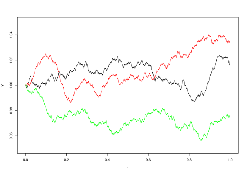
Figure 1. Three sample trajectories of the process $Y$ obtained by approximation scheme (15); $T=1$, $\kappa=1$, $\theta=1$, $\nu=0.14$, $Y_{0}=1$, $H=0.7$ and $\Delta_{n}=0.0001$.

For the sake of simplicity, instead of linear interpolation between the points of the partition, we put $\hat{Y}^{n}_{t}=\hat{Y}^{n}_{t^{n}_{k}}$ for $t\in[\hat{Y}^{n}_{t^{n}_{k}},\hat{Y}^{n}_{t^{n}_{k+1}})$. It should be noted that in this case speed of convergence of approximations remains the same as in Theorem 5.1 due to Remark 3.2 because

$$\mathbb{E}|Y_{t}-\hat{Y}^{n}_{t^{n}_{k}}|^{p}\leq 2^{p-1}(\mathbb{E}|Y_{t}-Y_{t^{n}_{k}}|^{p}+\mathbb{E}|Y_{t^{n}_{k}}-\hat{Y}^{n}_{t^{n}_{k}}|^{p}).$$

Denote

$$X_{t}:=\log S_{t}=X_{0}+\mu t-\frac{1}{2}\int_{0}^{t}\sigma^{2}(Y_{s})ds+\int_{0}^{t}\sigma(Y_{s})dW_{s},$$

where $X_{0}:=\log S_{0}$, and consider the discretized process

$$\hat{X}_{t_{k}^{n}}^{n} =X_{0}+\mu t_{k}^{n}-\frac{1}{2n}\sum_{j=0}^{k-1}\sigma^{2}(\hat{Y}^{n}_{t_{j}^{n}})+\sum_{j=0}^{k-1}\sigma(\hat{Y}^{n}_{t_{j}^{n}})\Delta W_{j}$$

$$=X_{0}+\mu t_{k}^{n}-\frac{1}{2}\int_{0}^{t_{k}^{n}}\sigma^{2}(\hat{Y}^{n}_{s})ds+\int_{0}^{t_{k}^{n}}\sigma(\hat{Y}^{n}_{s})dW_{s},\quad k=1,...,n,$$

where $\Delta W_{j}=W_{t_{j+1}^{n}}-W_{t_{j}^{n}}$.

Before going to the main theorem of the paper, let us prove several auxiliary results.

Theorem 5.2.

Let $p\geq 1$. Then, for all $H\in(0,1)$:

$$\sup_{n\geq 1}\sup_{t\in[0,T]}\mathbb{E}(\hat{Y}^{n}_{t})^{p}<\infty.$$

Remark 5.2.

Note that approximations (15) (see Fig. 2) are correctly defined for $H<1/2$ and Theorem 5.2 holds for an arbitrary Hurst parameter as well. However, for $H<1/2$ behaviour of $\hat{Y}^{n}$ as $n\to\infty$ remains obscure.

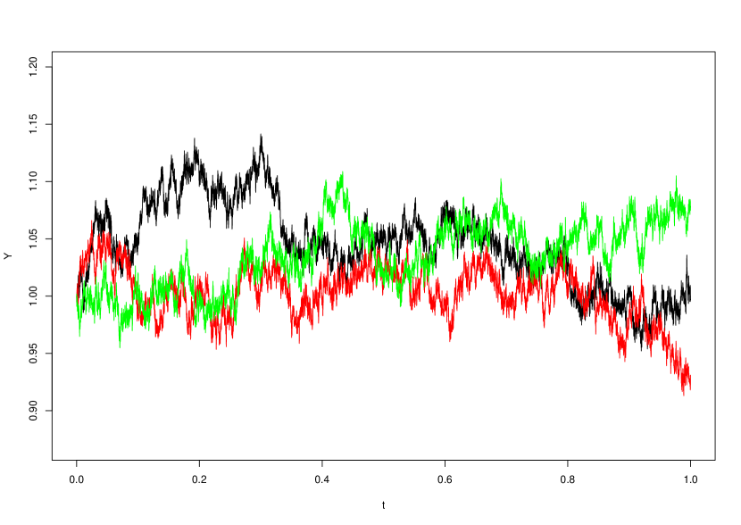
Figure 2. Three sample trajectories of the process $\hat{Y}^{n}$ for $H=0.3$, $T=1$, $\kappa=1$, $\theta=1$, $\nu=0.14$, $Y_{0}=1$ and $\Delta_{n}=0.0001$.

Corollary 5.1.

Approximating processes $\hat{Y}^{n}$ have bounded exponential moments, i.e. for any $x>0$ and $\varrho<2$:

$$\sup_{n\geq 1}\mathbb{E}\exp\left\{x\sup_{t\in[0,T]}(\hat{Y}^{n}_{t})^{\varrho}\right\}<\infty.$$

Remark 5.3.

From Theorem 5.2, Corollary 5.1 and Assumption 2 (ii), using the same argument as in the proof of Theorem 3.5, it is easy to verify that for any $m\in\mathbb{Z}$:

$$\begin{gathered}\sup_{n\geq 1}\sup_{t\in[0,T]}\mathbb{E}\left(\hat{S}^{n}_{t}\right)^{m}<\infty,\\ \sup_{n\geq 1}\sup_{t\in[0,T]}\mathbb{E}\exp\left\{m\left(\int_{0}^{t}\sigma(\hat{Y}^{n}_{s})dW_{s}-\frac{1}{2}\int_{0}^{t}\sigma^{2}(\hat{Y}^{n}_{s})ds\right)\right\}<\infty.\end{gathered}$$

Theorem 5.3.

Let $n\geq 2$ and conditions of Theorem 5.1 hold for $p=4$. Then, under Assumption 2, there exists a constant $C$ such that

(18) $$\mathbb{E}|X_{T}-\hat{X}^{n}_{T}|^{2}\leq C\Delta_{n}^{2rH},$$

(19) $$\mathbb{E}|Z_{T}-\hat{Z}^{n}_{T}|^{2}\leq C\Delta_{n}^{2rH},$$

where $\hat{Z}^{n}_{T}:=\int_{0}^{T}\sigma^{-1}(\hat{Y}^{n}_{u})d\tilde{V}_{u}$.

Lemma 5.1.

Let $n\geq 2$ and conditions of Theorem 5.1 hold for $p=32$. Then, under Assumptions 2 and 3, there is such $C_{F}>0$ that

$$\mathbb{E}\left|\frac{F(S_{T})}{S_{T}}-\frac{F(\hat{S}^{n}_{T})}{\hat{S}^{n}_{T}}\right|^{2}\leq C_{F}\Delta_{n}^{H}.$$

Theorem 5.4.

Let $n\geq 2$ and conditions of Theorem 5.1 for $p=32$ hold. Then, under Assumptions 2 and 3,

$$\left|\mathbb{E}f(S_{T})-\mathbb{E}\left[\frac{F(\hat{S}^{n}_{T})}{\hat{S}^{n}_{T}}\left(1+\frac{\hat{Z}^{n}_{T}}{T}\right)\right]\right|\leq C\Delta_{n}^{rH}.$$

6. Simulations

In this section, we use the discretization scheme studied previously to estimate option price for several payoff functions $f$. In all simulations we use $T=1$, $\kappa=1$, $\theta=1$ and $\nu=0.14$ to make sure that for all $H\in(1/2,1)$ the following condition is satisfied for $p=32$:

$$3p+1\leq\frac{2\kappa}{\nu^{2}HT^{2H-1}},$$

which is sufficient for Theorem 5.4 to hold true. For simplicity, we also consider everywhere the case $\mu=0.5$, $\rho=0$ and $\sigma=0.5\left(x+0.01\right)^{0.9}$.

In Tables 1–3 we present descriptive statistics of Monte-Carlo estimations of $\mathbb{E}\left[\frac{F(\hat{S}^{n}_{T})}{\hat{S}^{n}_{T}}\left(1+\frac{\hat{Z}^{n}_{T}}{T}\right)\right]$ (and, therefore, $\mathbb{E}f(S_{T})$) for different functions $f$ and different partition sizes $\Delta_{n}$. On Fig. 3, (a)–(c), the data is visualized in a form of box-and-whisker plots. In each case, 1000 Monte-Carlo estimates of option price, calculated from samples of 1000 trials each, were analyzed. All calculations were performed in R using package somebm to generate trajectories of Wiener process and fractional Brownian motion.

Table 1. $f(x)=(x-K)^{+}$, $K=1$, $\sigma(x)=0.5(x+0.01)^{0.9}$, $\mu=0.5$, $H=0.7$

$n$	Mean	Standard deviation	Coefficient of variation	Min.	1st Qu.	Median	3rd Qu.	Max.
100	0.7019	0.05628101	0.0802	0.5171	0.6630	0.7006	0.7380	0.8989
500	0.7040	0.05476103	0.0778	0.5406	0.6655	0.7025	0.7406	0.9305
1000	0.7004	0.05459163	0.0779	0.5463	0.6625	0.6978	0.7375	0.9344

Table 2. $f(x)=\mathbbm{1}_{[0.5,1]}(x)$, $\sigma(x)=0.5(x+0.01)^{0.9}$, $\mu=0.5$, $H=0.7$

$n$	Mean	Standard deviation	Coefficient of variation	Min.	1st Qu.	Median	3rd Qu.	Max.
100	0.2126	0.01196734	0.0563	0.1790	0.2046	0.2131	0.2206	0.2518
500	0.2123	0.01266216	0.0596	0.1652	0.2037	0.2124	0.2206	0.2553
1000	0.2129	0.01272749	0.0598	0.1725	0.2042	0.2132	0.2210	0.2505

Table 3. $f(x)=\mathbbm{1}_{(0.5,\infty)}(x)+\frac{1}{2}\sum_{k=2}^{6}\mathbbm{1}_{(0.5k,\infty)}(x)$, $\sigma(x)=0.5(x+0.01)^{0.9}$, $\mu=0.5$, $H=0.7$

$n$	Mean	Standard deviation	Coefficient of variation	Min.	1st Qu.	Median	3rd Qu.	Max.
100	1.804	0.08973507	0.0497	1.476	1.748	1.803	1.864	2.066
500	1.806	0.08873267	0.0491	1.546	1.745	1.805	1.866	2.136
1000	1.806	0.09001699	0.0498	1.547	1.747	1.809	1.865	2.105

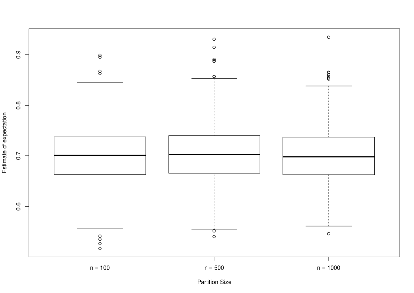
(a)

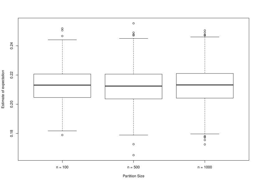
(b)

(c)

Figure 3. Box-and-whisker plots of Monte-Carlo estimates of $\mathbb{E}f(S_{T})$ using smoothed formula; in all cases $T=1$, $\kappa=1$, $\theta=1$, $\nu=0.14$, $\mu=0.5$, $\rho=0$, $\sigma=0.5\left(x+0.01\right)^{0.9}$, $H=0.7$; (a) $f(x)=(x-1)^{+}$, (b) $f(x)=\mathbbm{1}_{[0.5,1]}(x)$, (c) $f(x)=\mathbbm{1}_{(0.5,\infty)}(x)+\frac{1}{2}\sum_{k=2}^{6}\mathbbm{1}_{(0.5k,\infty)}(x)$

As we can see, simulations show relatively small coefficient of variation in all cases. Nota that increasing partition size does not lead to any significant changes in standard deviation of the estimates.

7. Proofs

Proof of Theorem 3.3. Denote $\alpha:=1-\beta$ and let $\varepsilon>0$ be fixed. By applying the chain rule, we obtain:

(20) $$(Y_{t}+\varepsilon)^{\alpha} =(Y_{t_{0}}+\varepsilon)^{\alpha}+\int_{t_{0}}^{t}\frac{\kappa\alpha}{2Y_{u}(Y_{u}+\varepsilon)^{1-\alpha}}du-\int_{t_{0}}^{t}\frac{\theta\alpha Y_{u}}{2(Y_{u}+\varepsilon)^{1-\alpha}}du$$

$$\quad+\int_{t_{0}}^{t}\frac{\nu\alpha}{2(Y_{u}+\varepsilon)^{1-\alpha}}dB_{u}^{H}.$$

It is clear from (3) that the process $Y=\{Y_{t},~{}t\in[0,T]\}$ has trajectories that are $\delta$-Hölder-continuous for any $\delta\in(0,H)$, so the process

$$\frac{\nu\alpha}{2(Y_{t}+\varepsilon)^{1-\alpha}},\quad t\in[0,T],$$

also has Hölder-continuous trajectories up to the order $H$. Therefore, the sum of Hölder exponents of the integrator and integrand in the integral w.r.t. fractional Brownian motion in (20) exceeds 1. In this case this integral is the pathwise limit of Riemann-Stieltjes integral sums (see, for example, [32]), coincides with the pathwise Stratonovich integral and, by applying Theorem A.1, we can rewrite (20) as follows:

(21) $$(Y_{t}+\varepsilon)^{\alpha} =(Y_{t_{0}}+\varepsilon)^{\alpha}+\int_{t_{0}}^{t}\frac{\kappa\alpha}{2Y_{u}(Y_{u}+\varepsilon)^{1-\alpha}}ds-\int_{t_{0}}^{t}\frac{\theta\alpha Y_{u}}{2(Y_{u}+\varepsilon)^{1-\alpha}}ds$$

$$\quad+H(2H-1)\int_{t_{0}}^{t}\int_{0}^{t}D_{s}^{H}\left[\frac{\nu\alpha}{2(Y_{u}+\varepsilon)^{1-\alpha}}\right]|u-s|^{2H-2}dsdu$$

$$\quad+\int_{t_{0}}^{t}\frac{\nu\alpha}{2(Y_{u}+\varepsilon)^{1-\alpha}}\delta B_{u}^{H},$$

where $D^{H}_{s}$ is the Malliavin derivative operator w.r.t. $B^{H}$ and $\int_{t_{0}}^{t}\frac{\nu\alpha}{2(Y(s)+\varepsilon)^{1-\alpha}}\delta B_{s}^{H}$ is the corresponding Skorokhod integral.

Note that

$$D_{s}^{H}Y_{u}= D_{s}^{H}\left[Y_{0}+\int_{0}^{u}\frac{\kappa}{2Y_{v}}dv-\frac{\theta}{2}\int_{0}^{u}Y_{v}dv+\frac{\nu}{2}B_{u}^{H}\right]=$$

$$= -\int_{0}^{u}\frac{\kappa D_{s}^{H}Y_{v}}{2Y^{2}_{v}}dv-\frac{\theta}{2}\int_{0}^{u}D_{s}^{H}Y_{v}dv+\frac{\nu}{2}\mathbbm{1}_{[0,u]}(s)$$

$$= -\int_{0}^{u}\left(\frac{\kappa}{2Y^{2}_{v}}+\frac{\theta}{2}\right)D_{s}^{H}Y_{v}dv+\frac{\nu}{2}\mathbbm{1}_{[0,u]}(s).$$

From this, it is easy to verify that

$$D_{s}^{H}Y_{u}=\frac{\nu}{2}\exp\left\{-\int_{s}^{u}\left(\frac{\kappa}{2Y^{2}_{v}}+\frac{\theta}{2}\right)dv\right\}\mathbbm{1}_{[0,u]}(s),$$

so

(22) $$D_{s}^{H}\left[\frac{\nu\alpha}{2(Y_{u}+\varepsilon)^{1-\alpha}}\right] =-\frac{\nu\alpha(1-\alpha)}{2(Y_{u}+\varepsilon)^{2-\alpha}}D_{s}^{H}Y_{u}$$

$$=-\frac{\nu^{2}\alpha(1-\alpha)}{4(Y_{u}+\varepsilon)^{2-\alpha}}\exp\left\{-\int_{s}^{u}\left(\frac{\kappa}{2Y^{2}_{v}}+\frac{\theta}{2}\right)dv\right\}\mathbbm{1}_{[0,u]}(s).$$

Taking into account (21) and (22), we can rewrite (20) in the following form:

(23) $$(Y_{t}+\varepsilon)^{\alpha} =(Y_{t_{0}}+\varepsilon)^{\alpha}+\int_{t_{0}}^{t}\frac{\kappa\alpha}{2Y_{u}(Y_{u}+\varepsilon)^{1-\alpha}}ds-\int_{t_{0}}^{t}\frac{\theta\alpha Y_{u}}{2(Y_{u}+\varepsilon)^{1-\alpha}}ds$$

$$\quad-\int_{t_{0}}^{t}\int_{0}^{u}\frac{\frac{\nu^{2}}{2}\alpha(1-\alpha)\exp\left\{-\int_{s}^{u}\left(\frac{\kappa}{2Y^{2}_{v}}+\frac{\theta}{2}\right)dv\right\}\varphi(u,s)ds}{2(Y_{u}+\varepsilon)^{2-\alpha}}du$$

$$\quad+\int_{t_{0}}^{t}\frac{\nu\alpha}{2(Y_{u}+\varepsilon)^{1-\alpha}}\delta B_{u}^{H},$$

where $\varphi(u,s):=H(2H-1)|u-s|^{2H-2}$.

Note that

(24) $$\begin{gathered}\int_{t_{0}}^{t}\frac{\kappa\alpha}{2Y_{u}(Y_{u}+\varepsilon)^{1-\alpha}}ds-\int_{t_{0}}^{t}\int_{0}^{u}\frac{\frac{\nu^{2}}{2}\alpha(1-\alpha)\exp\left\{-\int_{s}^{u}\left(\frac{\kappa}{2Y^{2}_{v}}+\frac{\theta}{2}\right)dv\right\}\varphi(u,s)ds}{2(Y_{u}+\varepsilon)^{2-\alpha}}du\\ \geq\alpha\int_{t_{0}}^{t}\frac{\kappa-(1-\alpha)\int_{0}^{u}\frac{\nu^{2}}{2}\exp\left\{-\int_{s}^{u}\left(\frac{\kappa}{2Y^{2}_{v}}+\frac{\theta}{2}\right)dv\right\}\varphi(u,s)ds}{2(Y_{u}+\varepsilon)^{2-\alpha}}du.\end{gathered}$$

It is easy to verify that

$$0 \geq-\int_{0}^{u}\exp\left\{-\int_{s}^{u}\left(\frac{\kappa}{2Y^{2}_{v}}+\frac{\theta}{2}\right)dv\right\}\varphi(u,s)ds$$

$$\geq-H(2H-1)\int_{0}^{u}|u-s|^{2H-2}ds$$

$$\geq-HT^{2H-1},$$

so

$$0\geq-(1-\alpha)\int_{0}^{u}\frac{\nu^{2}}{2}\exp\left\{-\int_{s}^{u}\left(\frac{\kappa}{2Y^{2}_{v}}+\frac{\theta}{2}\right)dv\right\}\varphi(u,s)ds\geq-(1-\alpha)\frac{\nu^{2}}{2}HT^{2H-1}.$$

Hence, if $\alpha\in\left(\max\{0,1-\frac{\kappa}{\nu^{2}HT^{2H-1}}\},1\right)$, i.e. when $0\geq-(1-\alpha)\frac{\nu^{2}}{2}HT^{2H-1}\geq-\frac{\kappa}{2}$,

$$\kappa-(1-\alpha)\int_{0}^{u}\frac{\nu^{2}}{2}\exp\left\{-\int_{s}^{u}\left(\frac{\kappa}{2Y^{2}_{v}}+\frac{\theta}{2}\right)dv\right\}\varphi(u,s)ds\geq\frac{\kappa}{2},$$

and

(25) $$\begin{gathered}\int_{t_{0}}^{t}\frac{\kappa\alpha}{2Y_{u}(Y_{u}+\varepsilon)^{1-\alpha}}ds-\int_{t_{0}}^{t}\int_{0}^{u}\frac{\frac{\nu^{2}}{2}\alpha(1-\alpha)\exp\left\{-\int_{s}^{u}\left(\frac{\kappa}{2Y^{2}_{v}}+\frac{\theta}{2}\right)dv\right\}\varphi(u,s)ds}{2(Y_{u}+\varepsilon)^{2-\alpha}}du\\ \geq\frac{\alpha\kappa}{4}\int_{t_{0}}^{t}\frac{1}{(Y_{u}+\varepsilon)^{2-\alpha}}du.\end{gathered}$$

Moreover,

(26) $$-\int_{t_{0}}^{t}\frac{\theta\alpha Y_{u}}{2(Y_{u}+\varepsilon)^{1-\alpha}}ds\geq-\frac{\theta\alpha}{2}\int_{t_{0}}^{t}(Y_{u}+\varepsilon)^{\alpha}du.$$

Therefore, taking into account upper bounds (24), (25) and (26), it is obvious from (23) that

$$(Y_{t}+\varepsilon)^{\alpha} \geq(Y_{t_{0}}+\varepsilon)^{\alpha}+\frac{\alpha\kappa}{4}\int_{t_{0}}^{t}\frac{1}{(Y_{u}+\varepsilon)^{2-\alpha}}du-\frac{\theta\alpha}{2}\int_{t_{0}}^{t}(Y_{u}+\varepsilon)^{\alpha}du$$

$$\quad+\int_{t_{0}}^{t}\frac{\nu\alpha}{2(Y_{u}+\varepsilon)^{1-\alpha}}\delta B_{u}^{H},$$

or

$$\int_{t_{0}}^{t}\frac{1}{(Y_{u}+\varepsilon)^{2-\alpha}}du\leq \frac{4}{\kappa\alpha}(Y_{t}+\varepsilon)^{\alpha}-\frac{4}{\kappa\alpha}(Y_{t_{0}}+\varepsilon)^{\alpha}+\frac{2\theta}{\kappa}\int_{t_{0}}^{t}(Y_{u}+\varepsilon)^{\alpha}du$$

$$-\frac{4}{\kappa\alpha}\int_{t_{0}}^{t}\frac{\nu\alpha}{2(Y_{u}+\varepsilon)^{1-\alpha}}\delta B_{u}^{H}.$$

Since the expectation of the Skorokhod integral is zero, by letting $\varepsilon\to 0$ we obtain that

(27) $$\mathbb{E}\left[\int_{t_{0}}^{t}\frac{1}{Y_{u}^{2-\alpha}}du\right]\leq\frac{4}{\kappa\alpha}\mathbb{E}(Y_{t}^{\alpha}-Y_{t_{0}}^{\alpha})+\frac{2\theta}{\kappa}\int_{t_{0}}^{t}\mathbb{E}Y_{u}^{\alpha}du.$$

Finiteness of the right-hand side of (27) follows from Theorem 3.1. $\square$
Proof of Theorem 3.4. From (3), Hölder’s and Jensen’s inequalities it is clear that

(28) $$\begin{gathered}\mathbb{E}|Y_{t}-Y_{s}|^{1+\beta}=\mathbb{E}\left|\int_{s}^{t}\frac{\kappa}{2Y_{u}}du-\frac{\theta}{2}\int_{s}^{t}Y_{u}du+\frac{\nu}{2}(B^{H}_{t}-B^{H}_{s})\right|^{1+\beta}\\ \leq 3^{\beta}\left(\left(\frac{\kappa}{2}\right)^{1+\beta}\mathbb{E}\left|\int_{s}^{t}\frac{1}{Y_{u}}du\right|^{1+\beta}+\left(\frac{\theta}{2}\right)^{1+\beta}\mathbb{E}\left|\int_{s}^{t}Y_{u}du\right|^{1+\beta}+\left(\frac{\nu}{2}\right)^{1+\beta}\mathbb{E}\left|B^{H}_{t}-B^{H}_{s}\right|^{1+\beta}\right)\\ \leq\tilde{C}_{1}(t-s)^{\beta}\mathbb{E}\int_{s}^{t}\frac{1}{Y_{u}^{1+\beta}}du+\tilde{C}_{2}(t-s)^{\beta}\mathbb{E}\int_{s}^{t}Y_{u}^{1+\beta}du+C_{3}|t-s|^{(1+\beta)H},\end{gathered}$$

where

$$\tilde{C}_{1}:=3^{\beta}\left(\frac{\kappa}{2}\right)^{1+\beta},\quad\tilde{C}_{2}:=3^{\beta}\left(\frac{\theta}{2}\right)^{1+\beta},\quad C_{3}:=(3\sqrt{2})^{\beta}\sqrt{\frac{2}{\pi}}\Gamma\left(1+\frac{\beta}{2}\right)\left(\frac{\nu}{2}\right)^{1+\beta}.$$

Note that form of $C_{3}$ follows from the fact that $B^{H}_{t}-B^{H}_{s}\sim\mathcal{N}(0,|t-s|^{2H})$ (see, for example, [30])

From Theorem 3.1 it is obvious that

(29) $$\tilde{C}_{2}(t-s)^{\beta}\mathbb{E}\int_{s}^{t}Y_{u}^{1+\beta}du\leq\tilde{C}_{2}\sup_{u\in[0,T]}\mathbb{E}\left[Y_{u}^{1+\beta}\right](t-s)^{1+\beta}=:C_{2}(t-s)^{1+\beta}.$$

Finally, from Theorem 3.3,

(30) $$\tilde{C}_{1}(t-s)^{\beta}\mathbb{E}\int_{s}^{t}\frac{1}{Y_{u}^{1+\beta}}du<C_{1}(t-s)^{\beta},$$

where $C_{1}=\tilde{C}_{1}\mathbb{E}\int_{s}^{t}\frac{1}{Y_{u}^{1+\beta}}du<C_{1}(t-s)^{\beta}$.

The statement of the Theorem now follows from (28), (29) and (30) as well as the fact that from condition $\beta<1$ it is easy to verify that for any $H\in(1/2,1)$:

$$\beta<(1+\beta)H.$$

$\square$
Proof of Theorem 3.5. 1. From Theorem 3.1, for all $\varrho\in[0,2)$:

$$\sup_{t\in[0,T]}|Y(t)|^{\varrho}\leq C_{1}+C_{2}\sup_{t\in[0,T]}|B^{H}_{t}|^{\varrho},$$

and, due to [13], for all $x>0$ and $\varrho\in[0,2)$:

$$\mathbb{E}\exp\left\{x\sup_{t\in[0,T]}|B^{H}_{t}|^{\varrho}\right\}<\infty.$$

Hence,

$$\exp\left\{x\sup_{t\in[0,T]}|Y_{t}|^{\varrho}\right\}\leq\exp\left\{C_{1}x+C_{2}x\sup_{t\in[0,T]}|B^{H}_{t}|^{\varrho}\right\}<\infty.$$

2. In order to show that the representation (8) indeed holds, it is sufficient to prove that the integrals $\int_{0}^{t}\sigma(Y_{s})dW_{s}$ and $\int_{0}^{t}\sigma(Y_{s})S_{s}dW_{s}$ are well-defined, while the form of the representation can be obtained straightforwardly.

Note that (see, for example, [24]) for all $p>0$

$$\mathbb{E}\sup_{s\in[0,T]}|B^{H}_{s}|^{p}<\infty,$$

so, due to item $(ii)$ from Assumption 2 and Theorem 3.1,

$$\int_{0}^{t}\mathbb{E}\sigma^{2}(Y_{s})ds\leq C^{2}_{\sigma}\int_{0}^{t}\mathbb{E}(1+|Y_{s}|^{q})^{2}ds\leq 2C^{2}_{\sigma}\int_{0}^{t}\mathbb{E}(1+|Y_{s}|^{2q})ds<\infty,$$

and the integral $\int_{0}^{t}\sigma(Y_{s})dW_{s}$ is well-defined.

Now consider the integral $\int_{0}^{t}\sigma(Y_{s})S_{s}dW_{s}$. As

(31) $$\begin{gathered}\int_{0}^{T}\mathbb{E}\left[\sigma^{2}(Y_{s})S^{2}_{s}\right]ds\leq\int_{0}^{T}\left(\mathbb{E}\sigma^{4}(Y_{s})\right)^{\frac{1}{2}}\left(\mathbb{E}S^{4}_{s}\right)^{\frac{1}{2}}ds\\ \leq T\sup_{s\in[0,T]}\left(\mathbb{E}\sigma^{4}(Y_{s})\right)^{\frac{1}{2}}\sup_{s\in[0,T]}\left(\mathbb{E}S^{4}_{s}\right)^{\frac{1}{2}},\end{gathered}$$

it is sufficient to check two conditions:

$$\begin{gathered}\sup_{s\in[0,T]}\left(\mathbb{E}\sigma^{4}(Y_{s})\right)^{\frac{1}{2}}<\infty,\qquad\sup_{s\in[0,T]}\left(\mathbb{E}S^{4}_{s}\right)^{\frac{1}{2}}<\infty.\end{gathered}$$

Using Theorem 3.1 and Assumption 2, $(ii)$, it is easy to verify that

(32) $$\begin{gathered}\sup_{s\in[0,T]}\left(\mathbb{E}\sigma^{4}(Y_{s})\right)^{\frac{1}{2}}\leq\sup_{s\in[0,T]}\left(C_{\sigma}^{4}\mathbb{E}(1+|Y_{s}|^{q})^{4}\right)^{\frac{1}{2}}\\ \leq\sup_{s\in[0,T]}\left(8C_{\sigma}^{4}\mathbb{E}(1+|Y_{s}|^{4q})\right)^{\frac{1}{2}}\leq\left(8C_{\sigma}^{4}+8C_{\sigma}^{4}\sup_{s\in[0,T]}\mathbb{E}|Y_{s}|^{4q}\right)^{\frac{1}{2}}<\infty.\end{gathered}$$

Moreover, from (7), for any $x>0$:

(33) $$\mathbb{E}\exp\left\{x\int_{0}^{t}\sigma^{2}(Y_{s})ds\right\} \leq\mathbb{E}\exp\left\{2xC_{\sigma}\int_{0}^{t}(1+|Y_{s}|^{2q})ds\right\}$$

$$\leq C\mathbb{E}\exp\left\{2xC_{\sigma}T\sup_{s\in[0,T]}|Y_{s}|^{2q}\right\}<\infty,$$

hence, for all $n\in\mathbb{Z}$, by putting $x:=\frac{4n^{2}}{2}$, we obtain the Novikov’s condition for the process $-2n\sigma(Y_{t})$, $t\in~{}[0,T]$.

Consequently,

(34) $$\mathbb{E}\exp\left\{2n\int_{0}^{t}\sigma(Y_{s})dW_{s}-2n^{2}\int_{0}^{t}\sigma^{2}(Y_{s})ds\right\}=1,$$

and so

(35) $$\begin{gathered}\sup_{t\in[0,T]}\mathbb{E}S_{t}^{n}\leq C\sup_{t\in[0,T]}\mathbb{E}\exp\left\{n\int_{0}^{t}\sigma(Y_{s})dW_{s}-\frac{n}{2}\int_{0}^{t}\sigma^{2}(Y_{s})ds\right\}\\ =C\sup_{t\in[0,T]}\mathbb{E}\left[\exp\left\{n\int_{0}^{t}\sigma(Y_{s})dW_{s}-n^{2}\int_{0}^{t}\sigma^{2}(Y_{s})ds\right\}\exp\left\{(n^{2}-\frac{n}{2})\int_{0}^{t}\sigma^{2}(Y_{s})ds\right\}\right]\\ \leq C\sup_{t\in[0,T]}\Bigg{[}\left(\mathbb{E}\exp\left\{2n\int_{0}^{t}\sigma(Y_{s})dW_{s}-n\int_{0}^{t}\sigma^{2}(Y_{s})ds\right\}\right)^{\frac{1}{2}}\times\\ \times\left(\mathbb{E}\exp\left\{(2n^{2}-n)\int_{0}^{t}\sigma^{2}(Y_{s})ds\right\}\right)^{\frac{1}{2}}\Bigg{]}\\ =C\sup_{t\in[0,T]}\left(\mathbb{E}\exp\left\{(2n^{2}-n)\int_{0}^{t}\sigma^{2}(Y_{s})ds\right\}\right)^{\frac{1}{2}}<\infty\end{gathered}$$

due to (33).

Therefore, from (31), (32) and (35),

$$\int_{0}^{T}\mathbb{E}\left[\sigma^{2}(Y_{s})S^{2}_{s}\right]ds<\infty$$

and so the integral $\int_{0}^{t}\sigma(Y_{s})S_{s}dW_{s}$ is well-defined. $\square$
Proof of Theorem 3.6. The proof is similar to the proof of Theorem 4 in [6].
Proof of Lemma 4.1. Item $(i)$ can be found in [6]. In particular, $D^{\tilde{V}}_{u}Y_{t}=0$ in $(ii)$ follows from independence of $Y$ and $V$.

Applying stochastic derivative operator to both parts of the integral form of (3), we get

(36) $$D^{V}_{u}Y_{t} =\frac{1}{2}\int_{0}^{t}D^{V}_{u}\left(\frac{\kappa}{Y_{s}}-\theta Y_{s}\right)ds+\nu D^{V}_{u}B^{H}_{t}$$

$$=-\frac{1}{2}\int\limits_{0}^{t}\left(\frac{\kappa}{Y^{2}_{s}}+\theta\right)D^{V}_{u}{Y_{s}}ds+\nu K(t,u)\mathbbm{1}_{[0,t]}(u)$$

$$=-\frac{1}{2}\int\limits_{0}^{t}h(s)D^{V}_{u}{Y_{s}}ds+\nu K(t,u)\mathbbm{1}_{[0,t]}(u).$$

Application of the chain rule with the function $F(x)=1/x$ can be justified by the same argument as in Remark 10 of [6], since $F$ is locally Lipschitz on $(0,\infty)$.

According to [26], Theorem 2, $Y$ does not hit zero a.s. Therefore $h$ is well defined a.s., and (36) means that for a fixed $u$, the process $\{Z_{t},t\in[0,t]\}$ defined by $Z_{t}:=D^{B}_{u}Y_{t}$ satisfies a random linear integral equation of the form

(37) $$Z_{t}=-\int\limits_{0}^{t}h(s)Z_{s}ds+\nu K(t,u)\mathbbm{1}_{[0,t]}(u).$$

This is a Volterra equation, and its solution is given by

(38) $$Z_{t}=\nu\left[K(t,u)-\int\limits_{u}^{t}K(s,u)h(s)\exp\left\{-\int\limits_{s}^{t}h(v)dv\right\}ds\right]\mathbbm{1}_{[0,t]}(u).$$

Note that $K$ is differentiable in the first argument ($\frac{\partial}{dt}K(t,s)$ is well defined for $t>s$), so (38) can be checked by substituting in (37) and taking derivatives of both sides.

Both derivatives in $(iii)$ are obtained by direct differentiation following the Malliavin derivative rules, see e.g. [23], Proposition 3.4. Since $Y$ is independent of $\tilde{V}$,

$$D_{u}^{\tilde{V}}X_{t}=\sqrt{1-\rho^{2}}D_{u}^{\tilde{V}}\int_{0}^{t}\sigma(Y_{s})d\tilde{V}_{s}=\sqrt{1-\rho^{2}}\sigma(Y_{u})\mathbbm{1}_{[0,t]}(u).$$

To find $D_{u}^{V}X_{t}$, we note that

$$D_{u}^{V}X_{t} =D_{u}^{V}\left[-\frac{1}{2}\int_{0}^{t}\sigma^{2}(Y_{s})ds+\sqrt{1-\rho^{2}}\int_{0}^{t}\sigma(Y_{s})d\tilde{V}_{s}+\rho\int_{0}^{t}\sigma(Y_{s})dV_{s}\right]$$

$$=-\int_{0}^{t}\sigma(Y_{s})\sigma^{\prime}(Y_{s})D_{u}^{V}Y_{s}ds+\sqrt{1-\rho^{2}}\int_{0}^{t}\sigma^{\prime}(Y_{s})D_{u}^{V}Y_{s}d\tilde{V}_{s}$$

$$\quad+\rho\int_{0}^{t}\sigma^{\prime}(Y_{s})D_{u}^{V}Y_{s}dV_{s}+\rho\sigma(Y_{u})\mathbbm{1}_{[0,t]}(u)$$

$$=\left(-\int_{u}^{t}\sigma(Y_{s})\sigma^{\prime}(Y_{s})D_{u}^{V}Y_{s}ds+\int_{u}^{t}\sigma^{\prime}(Y_{s})D_{u}^{V}Y_{s}dW_{s}+\rho\sigma(Y_{u})\right)\mathbbm{1}_{[0,t]}(u).$$

$\square$
Proof of Theorem 4.1. The result can be obtained by following the proof of Lemma 11 in [6], taking into account Lemma 4.1 and relation (35). $\square$
Proof of Theorem 5.2. First, note that for any fixed $n$ and $k=0,1,...,n$:

(39) $$\begin{gathered}(\hat{Y}^{n}_{t^{n}_{k+1}})^{p}=\left(\frac{\hat{Y}^{n}_{t^{n}_{k}}+\frac{\nu}{2}\Delta B^{H}_{k+1}+\sqrt{(\hat{Y}^{n}_{t^{n}_{k}}+\frac{\nu}{2}\Delta B^{H}_{k+1})^{2}+\kappa\Delta_{n}(2+\theta\Delta_{n})}}{2+\theta\Delta_{n}}\right)^{p}\\ \leq C\left((\hat{Y}^{n}_{t^{n}_{k}})^{p}+\left(\frac{\nu}{2}\right)^{p}|\Delta B^{H}_{k+1}|^{p}+\left((\hat{Y}^{n}_{t^{n}_{k}}+\frac{\nu}{2}\Delta B^{H}_{k+1})^{2}+\kappa\Delta_{n}(2+\theta\Delta_{n})\right)^{\frac{p}{2}}\right)\\ \leq C\left((\hat{Y}^{n}_{t^{n}_{k}})^{p}+|\Delta B^{H}_{k+1}|^{p}+|\hat{Y}^{n}_{t^{n}_{k}}+\frac{\nu}{2}\Delta B^{H}_{k+1}|^{p}+(\kappa\Delta_{n}(2+\theta\Delta_{n}))^{\frac{p}{2}}\right)\\ \leq C\left(1+(\hat{Y}^{n}_{t^{n}_{k}})^{p}+|\Delta B^{H}_{k+1}|^{p}\right)\\ \leq C\left(1+(\hat{Y}^{n}_{t^{n}_{k}})^{p}+\sup_{t\in[0,T]}|B^{H}_{t}|^{p}\right).\end{gathered}$$

By continuing calculations above recurrently and taking into account that $\hat{Y}^{n}_{t^{n}_{0}}=Y_{0}$, it is easy to see that there is such constant $C_{n}$ that

$$\sup_{t\in[0,T]}(\hat{Y}^{n}_{t})^{p}=\max_{k=0,...,n}(\hat{Y}^{n}_{t^{n}_{k}})^{p}<C_{n}(1+\sup_{t\in[0,T]}|B^{H}_{t}|^{p}).$$

Moreover, for any fixed $N$ there is such constant $C_{N}$ that

$$\sup_{1\leq n\leq N}\sup_{t\in[0,T]}\mathbb{E}(\hat{Y}^{n}_{t})^{p}=\max_{n=1,...,N}\max_{k=0,...,n}\mathbb{E}(\hat{Y}^{n}_{t^{n}_{k}})^{p}<C_{N}(1+\sup_{t\in[0,T]}|B^{H}_{t}|^{p}).$$

Let us prove that there is such $C>0$ (which does not depend on $n$) that

$$\sup_{n\geq 1}\sup_{t\in[0,T]}(\hat{Y}^{n}_{t})^{p}<C(1+\sup_{t\in[0,T]}|B^{H}_{t}|^{p}).$$

From calculations above, it will be enough to show that, for some $N\geq 1$,

$$\sup_{n>N}\sup_{t\in[0,T]}(\hat{Y}^{n}_{t})^{p}<C(1+\sup_{t\in[0,T]}|B^{H}_{t}|^{p}).$$

Let $n>2(8\theta)^{p}T^{p-1}$ be fixed. Consider the last moment of staying above level $Y_{0}/2$, i.e.

$$\tau_{1}:=\max\left\{k=1,...,n~{}|~{}\forall t^{n}_{l}\leq t^{n}_{k}:\hat{Y}^{n}_{t^{n}_{l}}\geq\frac{Y_{0}}{2}\right\}.$$

Let us prove that for any point of the partition $t^{n}_{k}$, $k=1,...,n$, the following inequality holds:

(40) $$(\hat{Y}^{n}_{t^{n}_{k}})^{p}\leq \left((4Y_{0})^{p}+\left(\frac{8\kappa T}{Y_{0}}\right)^{p}+(8\nu)^{p}\sup_{s\in[0,T]}|B^{H}_{s}|^{p}\right)$$

$$\quad+(8\theta)^{p}T^{p-1}\sum_{j=1}^{k}(\hat{Y}^{n}_{t^{n}_{j}})^{p}\Delta_{n}.$$

In order to do that, we will separately consider cases $t^{n}_{k}\leq t^{n}_{\tau_{1}}$ and $t^{n}_{k}>t^{n}_{\tau_{1}}$.

Step 1. Assume that $t^{n}_{k}\leq t^{n}_{\tau_{1}}$. Then, due to representation (16),

$$\begin{gathered}(\hat{Y}^{n}_{t^{n}_{k}})^{p}=\left(Y_{0}+\frac{1}{2}\sum_{j=1}^{k}\left(\frac{\kappa}{\hat{Y}^{n}_{t^{n}_{j}}}-\theta\hat{Y}^{n}_{t^{n}_{j}}\right)\Delta_{n}+\frac{\nu}{2}B^{H}_{t^{n}_{k}}\right)^{p}\\ \leq 4^{p-1}\left(Y_{0}^{p}+\left(\frac{1}{2}\sum_{j=1}^{k}\frac{\kappa}{\hat{Y}^{n}_{t^{n}_{j}}}\Delta_{n}\right)^{p}+\left(\frac{\theta}{2}\sum_{j=1}^{k}\hat{Y}^{n}_{t^{n}_{j}}\Delta_{n}\right)^{p}+\left(\frac{\nu}{2}\right)^{p}|B^{H}_{t^{n}_{k}}|^{p}\right).\end{gathered}$$

Note that for all $t^{n}_{k}\leq t^{n}_{\tau_{1}}$:

$$\left(\frac{1}{2}\sum_{j=1}^{k}\frac{\kappa}{\hat{Y}^{n}_{t^{n}_{j}}}\Delta_{n}\right)^{p}\leq\left(\sum_{j=1}^{k}\frac{\kappa}{Y_{0}}\Delta_{n}\right)^{p}\leq\left(\frac{\kappa T}{Y_{0}}\right)^{p}.$$

Moreover, from Jensen’s inequality,

$$\left(\frac{\theta}{2}\sum_{j=1}^{k}\hat{Y}^{n}_{t^{n}_{j}}\Delta_{n}\right)^{p}\leq\left(\frac{\theta}{2}\right)^{p}T^{p-1}\sum_{j=1}^{k}(\hat{Y}^{n}_{t^{n}_{j}})^{p}\Delta_{n}.$$

Finally,

$$\left(\frac{\nu}{2}\right)^{p}|B^{H}_{t^{n}_{k}}|^{p}\leq\left(\frac{\nu}{2}\right)^{p}\sup_{s\in[0,T]}|B^{H}_{s}|^{p}.$$

Hence, for all $t^{n}_{k}\leq t^{n}_{\tau_{1}}$:

$$\begin{gathered}(\hat{Y}^{n}_{t^{n}_{k}})^{p}\leq 4^{p-1}\left(Y_{0}^{p}+\left(\frac{\kappa T}{Y_{0}}\right)^{p}+\left(\frac{\theta}{2}\right)^{p}T^{p-1}\sum_{j=1}^{k}(\hat{Y}^{n}_{t^{n}_{j}})^{p}\Delta_{n}+\left(\frac{\nu}{2}\right)^{p}\sup_{s\in[0,T]}|B^{H}_{s}|^{p}\right)\\ \leq\left((4Y_{0})^{p}+\left(\frac{8\kappa T}{Y_{0}}\right)^{p}+(8\nu)^{p}\sup_{s\in[0,T]}|B^{H}_{s}|^{p}\right)+(8\theta)^{p}T^{p-1}\sum_{j=1}^{k}(\hat{Y}^{n}_{t^{n}_{j}})^{p}\Delta_{n}.\end{gathered}$$

Step 2. Assume that $\tau_{1}\neq n$, i.e. there are points of partition on the interval $(t^{n}_{\tau_{1}},T]$. From definition of $\tau_{1}$, $\hat{Y}^{n}_{t^{n}_{\tau_{1}}}\geq\frac{Y_{0}}{2}$ and for all points of the partition $t^{n}_{k}$ such that $t^{n}_{k}\in(t^{n}_{\tau_{1}},T]$:

$$\left\{l=1,...,n~{}|~{}t^{n}_{l}\in(t^{n}_{\tau_{1}},t^{n}_{k}],~{}\hat{Y}^{n}_{t^{n}_{l}}<\frac{Y_{0}}{2}\right\}\neq\emptyset.$$

Let $t^{n}_{k}\in(t^{n}_{\tau_{1}},T]$ be fixed and denote

$$\tau_{2}^{k}:=\max\left\{l=1,...,n~{}|~{}t^{n}_{l}\in(t^{n}_{\tau_{1}},t^{n}_{k}],~{}\hat{Y}^{n}_{t^{n}_{l}}<\frac{Y_{0}}{2}\right\}.$$

It is obvious that $t^{n}_{\tau_{1}}<t^{n}_{\tau_{2}^{k}}\leq t^{n}_{k}$ and $\hat{Y}^{n}_{t^{n}_{\tau_{2}^{k}}}<\frac{Y_{0}}{2}$, and

(41) $$\begin{gathered}(\hat{Y}^{n}_{t^{n}_{k}})^{p}=(\hat{Y}^{n}_{t^{n}_{k}}-\hat{Y}^{n}_{t^{n}_{\tau_{2}^{k}}}+\hat{Y}^{n}_{t^{n}_{\tau_{2}^{k}}})^{p}\leq 2^{p-1}\left(|\hat{Y}^{n}_{t^{n}_{k}}-\hat{Y}^{n}_{t^{n}_{\tau_{2}^{k}}}|^{p}+(\hat{Y}^{n}_{t^{n}_{\tau_{2}^{k}}})^{p}\right)\\ \leq 2^{p-1}\left(|\hat{Y}^{n}_{t^{n}_{k}}-\hat{Y}^{n}_{t^{n}_{\tau_{2}^{k}}}|^{p}+\left(\frac{Y_{0}}{2}\right)^{p}\right)\leq 2^{p-1}|\hat{Y}^{n}_{t^{n}_{k}}-\hat{Y}^{n}_{t^{n}_{\tau_{2}^{k}}}|^{p}+Y_{0}^{p}.\end{gathered}$$

In addition, if $t^{n}_{\tau_{2}^{k}}=t^{n}_{k}$,

$$|\hat{Y}^{n}_{t^{n}_{k}}-\hat{Y}^{n}_{t^{n}_{\tau_{2}^{k}}}|^{p}=0,$$

and if $t^{n}_{\tau_{2}^{k}}<t^{n}_{k}$,

$$\begin{gathered}\left|\hat{Y}^{n}_{t^{n}_{k}}-\hat{Y}^{n}_{t^{n}_{\tau_{2}^{k}}}\right|^{p}=\left|\frac{1}{2}\sum_{j=\tau_{2}^{k}+1}^{k}\left(\frac{\kappa}{\hat{Y}^{n}_{t^{n}_{j}}}-\theta\hat{Y}^{n}_{t^{n}_{j}}\right)\Delta_{n}+\frac{\nu}{2}\left(B^{H}_{t^{n}_{k}}-B^{H}_{t^{n}_{\tau_{2}^{k}}}\right)\right|^{p}\\ \leq 4^{p-1}\left(\left(\frac{1}{2}\sum_{j=\tau_{2}^{k}+1}^{k}\frac{\kappa}{\hat{Y}^{n}_{t^{n}_{j}}}\Delta_{n}\right)^{p}+\left(\frac{\theta}{2}\sum_{j=\tau_{2}^{k}+1}^{k}\hat{Y}^{n}_{t^{n}_{j}}\Delta_{n}\right)^{p}+\left(\frac{\nu}{2}\right)^{p}|B^{H}_{t^{n}_{k}}|^{p}+\left(\frac{\nu}{2}\right)^{p}|B^{H}_{t^{n}_{\tau_{2}^{k}}}|^{p}\right).\end{gathered}$$

From definition of $\tau_{2}^{k}$, for all points of the partition $t^{n}_{l}\in(t^{n}_{\tau_{2}^{k}},t^{n}_{k}]$ it holds that $\hat{Y}^{n}_{t^{n}_{k}}\geq\frac{Y_{0}}{2}$, so

$$\left(\frac{1}{2}\sum_{j=\tau_{2}^{k}+1}^{k}\frac{\kappa}{\hat{Y}^{n}_{t^{n}_{j}}}\Delta_{n}\right)^{p}\leq\left(\frac{\kappa T}{Y_{0}}\right)^{p}.$$

Furthermore,

$$\left(\frac{\theta}{2}\sum_{j=\tau_{2}^{k}+1}^{k}\hat{Y}^{n}_{t^{n}_{j}}\Delta_{n}\right)^{p}\leq\left(\frac{\theta}{2}\right)^{p}T^{p-1}\sum_{j=1}^{k}(\hat{Y}^{n}_{t^{n}_{j}})^{p}\Delta_{n},$$

and

$$\left(\frac{\nu}{2}\right)^{p}|B^{H}_{t^{n}_{k}}|^{p}+\left(\frac{\nu}{2}\right)^{p}|B^{H}_{t^{n}_{\tau_{2}^{k}}}|^{p}\leq 2\left(\frac{\nu}{2}\right)^{p}\sup_{s\in[0,T]}|B^{H}_{s}|^{p}.$$

Hence,

(42) $$\begin{gathered}\left|\hat{Y}^{n}_{t^{n}_{k}}-\hat{Y}^{n}_{t^{n}_{\tau_{2}^{k}}}\right|^{p}\leq\\ \leq 4^{p-1}\left(\left(\frac{\kappa T}{Y_{0}}\right)^{p}+\left(\frac{\theta}{2}\right)^{p}T^{p-1}\sum_{j=1}^{k}(\hat{Y}^{n}_{t^{n}_{j}})^{p}\Delta_{n}+2\left(\frac{\nu}{2}\right)^{p}\sup_{s\in[0,T]}|B^{H}_{s}|^{p}\right).\end{gathered}$$

Finally, from (41) and (42),

$$\begin{gathered}(\hat{Y}^{n}_{t^{n}_{k}})^{p}\leq 8^{p-1}\left(\left(\frac{\kappa T}{Y_{0}}\right)^{p}+\left(\frac{\theta}{2}\right)^{p}T^{p-1}\sum_{j=1}^{k}(\hat{Y}^{n}_{t^{n}_{j}})^{p}\Delta_{n}+2\left(\frac{\nu}{2}\right)^{p}\sup_{s\in[0,T]}|B^{H}_{s}|^{p}\right)+Y_{0}^{p}\\ \leq\left((4Y_{0})^{p}+\left(\frac{8\kappa T}{Y_{0}}\right)^{p}+(8\nu)^{p}\sup_{s\in[0,T]}|B^{H}_{s}|^{p}\right)+(8\theta)^{p}T^{p-1}\sum_{j=1}^{k}(\hat{Y}^{n}_{t^{n}_{j}})^{p}\Delta_{n}.\end{gathered}$$

Therefore, (40) indeed holds for any point $t^{n}_{k}$ of the partition.

Step 3. As $n>2(8\theta)^{p}T^{p-1}$,

$$\frac{1}{2}\leq 1-(8\theta)^{p}T^{p-1}\Delta_{n}\leq 1,$$

therefore, as, due to (40),

$$\begin{gathered}\left(1-(8\theta)^{p}T^{p-1}\Delta_{n}\right)(\hat{Y}^{n}_{t^{n}_{k}})^{p}\\ \leq\left((4Y_{0})^{p}+\left(\frac{8\kappa T}{Y_{0}}\right)^{p}+(8\nu)^{p}\sup_{s\in[0,T]}|B^{H}_{s}|^{p}\right)+(8\theta)^{p}T^{p-1}\sum_{j=1}^{k-1}(\hat{Y}^{n}_{t^{n}_{j}})^{p}\Delta_{n},\end{gathered}$$

we have

$$\begin{gathered}(\hat{Y}^{n}_{t^{n}_{k}})^{p}\leq 2\left((4Y_{0})^{p}+\left(\frac{8\kappa T}{Y_{0}}\right)^{p}+(8\nu)^{p}\sup_{s\in[0,T]}|B^{H}_{s}|^{p}\right)+2(8\theta)^{p}T^{p-1}\sum_{j=1}^{k-1}(\hat{Y}^{n}_{t^{n}_{j}})^{p}\Delta_{n}.\end{gathered}$$

Using the discrete version of the Grönwall’s lemma, we obtain:

$$(\hat{Y}^{n}_{t^{n}_{k}})^{p}\leq 2\left((4Y_{0})^{p}+\left(\frac{8\kappa T}{Y_{0}}\right)^{p}+(8\nu)^{p}\sup_{s\in[0,T]}|B^{H}_{s}|^{p}\right)e^{2(8\theta T)^{p}},$$

i.e., taking into account that the right-hand side does not depend on $n$ and remarks in the beginning of the proof, there is such $C>0$ that

(43) $$\sup_{n\geq 0}\sup_{t\in[0,T]}(\hat{Y}^{n}_{t})^{p}<C(1+\sup_{t\in[0,T]}|B^{H}_{t}|^{p}).$$

Now the claim of the Theorem follows from the fact that the right-hand side of (43) does not depend on $n$ and that (see, for example, [24])

$$\mathbb{E}\sup_{s\in[0,T]}|B^{H}_{s}|^{p}<\infty.$$

$\square$
Proof of Corollary 5.1. From (43) it follows that there is such $C>0$ that

$$\sup_{n\geq 0}\sup_{t\in[0,T]}(\hat{Y}^{n}_{t})^{\varrho}<C(1+\sup_{t\in[0,T]}|B^{H}_{t}|^{\varrho}).$$

The rest of the proof is similar to Theorem 3.5, 1. $\square$
Proof of Theorem 5.3. We shall proceed as in proof of Lemma 14, [6].

Using Hölder’s inequality, we write:

$$\begin{gathered}\mathbb{E}|X_{T}-\hat{X}^{n}_{T}|^{2}=\mathbb{E}\left|-\frac{1}{2}\int_{0}^{T}\sigma^{2}(Y_{s})ds+\int_{0}^{T}\sigma(Y_{s})dW_{s}+\frac{1}{2}\int_{0}^{T}\sigma^{2}(\hat{Y}^{n}_{s})ds-\int_{0}^{T}\sigma(\hat{Y}^{n}_{s})dW_{s}\right|^{2}\\ \leq C\left(\mathbb{E}\left|-\frac{1}{2}\int_{0}^{T}(\sigma^{2}(Y_{s})-\sigma^{2}(\hat{Y}^{n}_{s}))ds\right|^{2}+\mathbb{E}\left|\int_{0}^{T}(\sigma(Y_{s})-\sigma(\hat{Y}^{n}_{s}))dW_{s}\right|^{2}\right)\\ \leq C\left(\int_{0}^{T}\mathbb{E}[\sigma^{2}(Y_{s})-\sigma^{2}(\hat{Y}^{n}_{s})]^{2}ds+\int_{0}^{T}\mathbb{E}[\sigma(Y_{s})-\sigma(\hat{Y}^{n}_{s})]^{2}ds\right)\\ =C\left(\int_{0}^{T}\mathbb{E}[(\sigma(Y_{s})-\sigma(\hat{Y}^{n}_{s}))(\sigma(Y_{s})+\sigma(\hat{Y}^{n}_{s}))]^{2}ds+\int_{0}^{T}\mathbb{E}[\sigma(Y_{s})-\sigma(\hat{Y}^{n}_{s})]^{2}ds\right).\end{gathered}$$

From Assumption 2 (iii), Jensen’s inequality and Theorem 5.1,

$$\int_{0}^{T}\mathbb{E}[\sigma(Y_{s})-\sigma(\hat{Y}^{n}_{s})]^{2}ds \leq C_{\sigma}^{2}\int_{0}^{T}\mathbb{E}[(Y_{s}-\hat{Y}^{n}_{s})^{2r}]ds$$

$$\leq C_{\sigma}^{2}\int_{0}^{T}\left(\mathbb{E}[(Y_{s}-\hat{Y}^{n}_{s})^{4}]\right)^{\frac{r}{2}}ds$$

$$\leq C\Delta_{n}^{2rH}.$$

Moreover, Assumption 2, (ii) and (iii), implies that

$$\begin{gathered}\mathbb{E}\left[\left(\sigma(Y_{s})-\sigma(\hat{Y}^{n}_{s})\right)\left(\sigma(Y_{s})+\sigma(\hat{Y}^{n}_{s})\right)\right]^{2}\leq C^{2}_{\sigma}\mathbb{E}\left[(Y_{s}-\hat{Y}^{n}_{s})^{2r}\left(2\sigma^{2}(Y_{s})+2\sigma^{2}(\hat{Y}^{n}_{s})\right)\right]\\ \leq C\mathbb{E}\left[(Y_{s}-\hat{Y}^{n}_{s})^{2r}\left((1+Y^{q}_{s})^{2}+(1+(\hat{Y}^{n}_{s})^{q})^{2}\right)\right]\\ \leq C\mathbb{E}\left[(Y_{s}-\hat{Y}^{n}_{s})^{2r}\left(1+Y^{2q}_{s}+(\hat{Y}^{n}_{s})^{2q}\right)\right]\\ \leq C\left(\mathbb{E}(Y_{s}-\hat{Y}^{n}_{s})^{4r}\right)^{\frac{1}{2}}\left(\mathbb{E}\left[1+Y^{4q}_{s}+(\hat{Y}^{n}_{s})^{4q}\right]\right)^{\frac{1}{2}}.\end{gathered}$$

From Theorem 5.1,

$$\left(\mathbb{E}(Y_{s}-\hat{Y}^{n}_{s})^{4r}\right)^{\frac{1}{2}}\leq\left(\mathbb{E}(Y_{s}-\hat{Y}^{n}_{s})^{4}\right)^{\frac{r}{2}}\leq C\Delta_{n}^{2rH},$$

and, from Theorems 3.1 and 5.2,

$$\left(\mathbb{E}\left[1+Y^{4q}_{s}+(\hat{Y}^{n}_{s})^{4q}\right]\right)^{1/2}<\infty.$$

Therefore, taking into account bounds above, there is such constant $C>0$ that

$$\mathbb{E}|X_{T}-\hat{X}^{n}_{T}|^{2}\leq C\Delta^{2rH}.$$

Now, let us prove (19). Taking into account Assumption 2 (i),

$$\left|\frac{1}{\sigma(x)}-\frac{1}{\sigma(y)}\right|=\frac{|\sigma(x)-\sigma(y)|}{\sigma(x)\sigma(y)}\leq\frac{|\sigma(x)-\sigma(y)|}{\sigma^{2}_{\min}},$$

so, from Assumption 2 (iii),

$$\mathbb{E}(Z_{T}-\hat{Z}^{n}_{T})^{2} =\int_{0}^{T}\mathbb{E}\left(\frac{1}{\sigma(Y_{s})}-\frac{1}{\sigma(\hat{Y}^{n}_{s})}\right)^{2}ds$$

$$\leq\frac{1}{\sigma^{2}_{\min}}C_{\sigma}\int_{0}^{T}\mathbb{E}(Y_{s}-\hat{Y}^{n}_{s})^{2r}ds$$

$$\leq C\int_{0}^{T}\left(\mathbb{E}(Y_{s}-\hat{Y}^{n}_{s})^{4}\right)^{\frac{r}{2}}ds$$

$$\leq C\Delta_{n}^{2rH}.$$

$\square$
Proof of Lemma 5.1. It is clear that

(44) $$\mathbb{E}\left|\frac{F(S_{T})}{S_{T}}-\frac{F(\hat{S}^{n}_{T})}{\hat{S}^{n}_{T}}\right|^{2}\leq 2\mathbb{E}\left|\frac{F(S_{T})}{S_{T}}-\frac{F(S_{T})}{\hat{S}^{n}_{T}}\right|^{2}+2\mathbb{E}\left|\frac{F(S_{T})}{\hat{S}^{n}_{T}}-\frac{F(\hat{S}^{n}_{T})}{\hat{S}^{n}_{T}}\right|^{2}.$$

Now we shall estimate the right-hand side of (44) term by term.

$$\mathbb{E}\left|F(S_{T})\left(\frac{1}{S_{T}}-\frac{1}{\hat{S}^{n}_{T}}\right)\right|^{2}\leq\left(\mathbb{E}\left(F(S_{T})\right)^{4}\mathbb{E}\left(\frac{1}{S_{T}}-\frac{1}{\hat{S}^{n}_{T}}\right)^{4}\right)^{\frac{1}{2}}.$$

From Assumption 3 (i), both $f$ and $F$ are of polynomial growth, therefore, due to (35),

$$\mathbb{E}\left(F(S_{T})\right)^{4}<\infty.$$

Furthermore, using sequentially the inequalities

$$\begin{gathered}|e^{x}-e^{y}|\leq(e^{x}+e^{y})|x-y|,\quad x,y\in\mathbb{R},\\ (x+y)^{2n}\leq C(n)(x^{2n}+y^{2n}),\quad x,y\in\mathbb{R},\quad n\in\mathbb{N}.\end{gathered}$$

and Hölder’s inequality, we obtain that

$$\begin{gathered}\mathbb{E}\left(\frac{1}{S_{T}}-\frac{1}{\hat{S}^{n}_{T}}\right)^{4}=\frac{1}{S_{0}^{4}e^{4\mu t}}\mathbb{E}\left[e^{\frac{1}{2}\int_{0}^{T}\sigma^{2}(Y_{s})ds-\int_{0}^{T}\sigma(Y_{s})dW_{s}}-e^{\frac{1}{2}\int_{0}^{T}\sigma^{2}(\hat{Y}^{n}_{s})ds-\int_{0}^{T}\sigma(\hat{Y}^{n}_{s})dW_{s}}\right]^{4}\\ \leq C\mathbb{E}\Bigg{[}\left(e^{\frac{1}{2}\int_{0}^{T}\sigma^{2}(Y_{s})ds-\int_{0}^{T}\sigma(Y_{s})dW_{s}}+e^{\frac{1}{2}\int_{0}^{T}\sigma^{2}(\hat{Y}^{n}_{s})ds-\int_{0}^{T}\sigma(\hat{Y}^{n}_{s})dW_{s}}\right)^{4}\\ \times\bigg{(}\frac{1}{2}\int_{0}^{T}\sigma^{2}(Y_{s})ds-\int_{0}^{T}\sigma(Y_{s})dW_{s}-\frac{1}{2}\int_{0}^{T}\sigma^{2}(\hat{Y}^{n}_{s})ds+\int_{0}^{T}\sigma(\hat{Y}^{n}_{s})dW_{s}\bigg{)}^{4}\Bigg{]}\\ \leq C\mathbb{E}\Bigg{[}\left(e^{2\int_{0}^{T}\sigma^{2}(Y_{s})ds-4\int_{0}^{T}\sigma(Y_{s})dW_{s}}+e^{2\int_{0}^{T}\sigma^{2}(\hat{Y}^{n}_{s})ds-4\int_{0}^{T}\sigma(\hat{Y}^{n}_{s})dW_{s}}\right)\\ \times\bigg{(}\frac{1}{2}\int_{0}^{T}\sigma^{2}(Y_{s})ds-\int_{0}^{T}\sigma(Y_{s})dW_{s}-\frac{1}{2}\int_{0}^{T}\sigma^{2}(\hat{Y}^{n}_{s})ds+\int_{0}^{T}\sigma(\hat{Y}^{n}_{s})dW_{s}\bigg{)}^{4}\Bigg{]}\\ \leq C\left(\mathbb{E}\left[e^{4\int_{0}^{T}\sigma^{2}(Y_{s})ds-8\int_{0}^{T}\sigma(Y_{s})dW_{s}}+e^{4\int_{0}^{T}\sigma^{2}(\hat{Y}^{n}_{s})ds-8\int_{0}^{T}\sigma(\hat{Y}^{n}_{s})dW_{s}}\right]\right)^{\frac{1}{2}}\\ \times\left(\mathbb{E}\left[\bigg{(}\frac{1}{2}\int_{0}^{T}\sigma^{2}(Y_{s})ds-\int_{0}^{T}\sigma(Y_{s})dW_{s}-\frac{1}{2}\int_{0}^{T}\sigma^{2}(\hat{Y}^{n}_{s})ds+\int_{0}^{T}\sigma(\hat{Y}^{n}_{s})dW_{s}\bigg{)}^{8}\right]\right)^{\frac{1}{2}}.\end{gathered}$$

Next, from (34) and Remark 5.3 it follows that

$$\begin{gathered}\mathbb{E}\left[e^{4\int_{0}^{T}\sigma^{2}(Y_{s})ds-8\int_{0}^{T}\sigma(Y_{s})dW_{s}}\right]<\infty,\\ \mathbb{E}\left[e^{4\int_{0}^{T}\sigma^{2}(\hat{Y}^{n}_{s})ds-8\int_{0}^{T}\sigma(\hat{Y}^{n}_{s})dW_{s}}\right]<\infty,\end{gathered}$$

so, using this together with Hölder and Burkholder-Davis-Gundy inequalities, we continue the chain as follows:

$$\begin{gathered}\mathbb{E}\left(\frac{1}{S_{T}}-\frac{1}{\hat{S}^{n}_{T}}\right)^{4}\\ \leq C\left(\mathbb{E}\left[\bigg{(}\frac{1}{2}\int_{0}^{T}\sigma^{2}(Y_{s})ds-\int_{0}^{T}\sigma(Y_{s})dW_{s}-\frac{1}{2}\int_{0}^{T}\sigma^{2}(\hat{Y}^{n}_{s})ds+\int_{0}^{T}\sigma(\hat{Y}^{n}_{s})dW_{s}\bigg{)}^{8}\right]\right)^{\frac{1}{2}}\\ \leq C\left(\mathbb{E}\left[\bigg{(}\int_{0}^{T}\sigma^{2}(Y_{s})ds-\int_{0}^{T}\sigma^{2}(\hat{Y}^{n}_{s})ds\bigg{)}^{8}\right]+\mathbb{E}\left[\bigg{(}\int_{0}^{T}\sigma(Y_{s})dW_{s}-\int_{0}^{T}\sigma(\hat{Y}^{n}_{s})dW_{s}\bigg{)}^{8}\right]\right)^{\frac{1}{2}}\\ \leq C\left(\mathbb{E}\left[\int_{0}^{T}\left(\sigma^{2}(Y_{s})-\sigma^{2}(\hat{Y}^{n}_{s})\right)^{8}ds\right]+\mathbb{E}\left[\left(\int_{0}^{T}\left(\sigma(Y_{s})-\sigma(\hat{Y}^{n}_{s})\right)^{2}ds\right)^{4}\right]\right)^{\frac{1}{2}}\\ \leq C\Bigg{(}\int_{0}^{T}\mathbb{E}\left(\left(\sigma(Y_{s})-\sigma(\hat{Y}^{n}_{s})\right)\left(\sigma(Y_{s})+\sigma(\hat{Y}^{n}_{s})\right)\right)^{8}ds\\ +\int_{0}^{T}\mathbb{E}\left(\sigma(Y_{s})-\sigma(\hat{Y}^{n}_{s})\right)^{8}ds\Bigg{)}^{\frac{1}{2}}.\end{gathered}$$

By applying Assumption 2, (ii) and (iii),

$$\begin{gathered}\int_{0}^{T}\mathbb{E}\left(\left(\sigma(Y_{s})-\sigma(\hat{Y}^{n}_{s})\right)\left(\sigma(Y_{s})+\sigma(\hat{Y}^{n}_{s})\right)\right)^{8}ds\\ \leq C\int_{0}^{T}\mathbb{E}\left[\left(Y_{s}-\hat{Y}^{n}_{s}\right)^{8r}\left(1+Y_{s}^{q}+(\hat{Y}^{n}_{s})^{q}\right)^{8}\right]ds\\ \leq C\int_{0}^{T}\left(\mathbb{E}\left[\left(Y_{s}-\hat{Y}^{n}_{s}\right)^{16r}\right]\right)^{\frac{1}{2}}\left(\mathbb{E}\left[1+Y_{s}^{16q}+(\hat{Y}^{n}_{s})^{16q}\right]\right)^{\frac{1}{2}}ds\end{gathered}$$

and

$$\begin{gathered}\int_{0}^{T}\mathbb{E}\left(\sigma(Y_{s})-\sigma(\hat{Y}^{n}_{s})\right)^{8}ds\leq C\int_{0}^{T}\mathbb{E}\left(Y_{s}-\hat{Y}^{n}_{s}\right)^{8r}ds.\end{gathered}$$

From Theorems 3.1 and 5.2,

$$\begin{gathered}\sup_{n\geq 1}\sup_{t\in[0,T]}\mathbb{E}\left[1+Y_{s}^{16q}+(\hat{Y}^{n}_{s})^{16q}\right]<\infty,\end{gathered}$$

and, according from Theorem 5.1,

$$\begin{gathered}\int_{0}^{T}\left(\mathbb{E}\left[\left(Y_{s}-\hat{Y}^{n}_{s}\right)^{16r}\right]\right)^{\frac{1}{2}}ds\leq C\Delta_{n}^{16rH}\\ \int_{0}^{T}\mathbb{E}\left(Y_{s}-\hat{Y}^{n}_{s}\right)^{8r}ds\leq C\Delta_{n}^{8rH},\end{gathered}$$

hence

(45) $$\begin{gathered}\mathbb{E}\left(\frac{1}{S_{T}}-\frac{1}{\hat{S}^{n}_{T}}\right)^{4}\leq C\Delta_{n}^{4rH}\leq C\Delta_{n}^{2rH}.\end{gathered}$$

Now, let us move to the second term of the right-hand side of (44).

$$\begin{gathered}\mathbb{E}\left|\frac{F(S_{T})}{\hat{S}^{n}_{T}}-\frac{F(\hat{S}^{n}_{T})}{\hat{S}^{n}_{T}}\right|^{2}\leq\left(\mathbb{E}\left[\frac{1}{(\hat{S}^{n}_{T})^{4}}\right]\right)^{\frac{1}{2}}\left(\mathbb{E}\left(F(S_{T})-F(\hat{S}^{n}_{T})\right)^{4}\right)^{\frac{1}{2}}.\end{gathered}$$

Due to Remark 5.3,

$$\mathbb{E}\left[\frac{1}{(\hat{S}^{n}_{T})^{4}}\right]<\infty,$$

and, from Assumption 3 (i),

$$\begin{gathered}\left(\mathbb{E}\left(F(S_{T})-F(\hat{S}^{n}_{T})\right)^{4}\right)^{\frac{1}{2}}=\left(\mathbb{E}\left(\int_{S_{T}\wedge\hat{S}^{n}_{T}}^{S_{T}\vee\hat{S}^{n}_{T}}f(x)dx\right)^{4}\right)^{\frac{1}{2}}\\ \leq C\left(\mathbb{E}\left[(S_{T}-\hat{S}^{n}_{T})^{4}(1+S_{T}^{p}+(\hat{S}^{n}_{T})^{p})^{4}\right]\right)^{\frac{1}{2}}\leq C\left(\mathbb{E}((S_{T}-\hat{S}^{n}_{T})^{8}\mathbb{E}(1+S_{T}^{p}+(\hat{S}^{n}_{T})^{p})^{8}\right)^{\frac{1}{4}}.\end{gathered}$$

According to (35) and Remark 5.3,

$$\mathbb{E}(1+S_{T}^{p}+(\hat{S}^{n}_{T})^{p})^{8}<\infty,$$

so

$$\mathbb{E}\left|\frac{F(S_{T})}{\hat{S}^{n}_{T}}-\frac{F(\hat{S}^{n}_{T})}{\hat{S}^{n}_{T}}\right|^{2}\leq C\left(\mathbb{E}((S_{T}-\hat{S}^{n}_{T})^{8}\right)^{\frac{1}{4}}.$$

To get the final result, we can proceed just as in the upper bound for the first term in the right-hand side of (44). Thus

(46) $$\begin{gathered}\mathbb{E}\left|\frac{F(S_{T})}{\hat{S}^{n}_{T}}-\frac{F(\hat{S}^{n}_{T})}{\hat{S}^{n}_{T}}\right|^{2}\leq C\left(\int_{0}^{T}\left(\left(\mathbb{E}|Y_{s}-\hat{Y}^{n}_{s}|^{32r}\right)^{\frac{1}{2}}+\mathbb{E}|Y_{s}-\hat{Y}^{n}_{s}|^{16r}\right)ds\right)^{\frac{1}{8}}\\ \leq C\Delta_{n}^{2rH}.\end{gathered}$$

Relations (45) and (46) together with (44) complete the proof. $\square$
Proof of Theorem 5.4. According to Theorem 4.1,

$$\begin{gathered}\left|\mathbb{E}f(S_{T})-\mathbb{E}\left[\frac{F(\hat{S}^{n}_{T})}{\hat{S}^{n}_{T}}\left(1+\frac{\hat{Z}^{n}_{T}}{T}\right)\right]\right|=\left|\mathbb{E}\left[\frac{F(S_{T})}{S_{T}}\left(1+\frac{Z_{T}}{T}\right)\right]-\mathbb{E}\left[\frac{F(\hat{S}^{n}_{T})}{\hat{S}^{n}_{T}}\left(1+\frac{\hat{Z}^{n}_{T}}{T}\right)\right]\right|\\ \leq\frac{1}{T}\mathbb{E}\left[\left|\frac{F(S_{T})}{S_{T}}(Z_{T}-\hat{Z}^{n}_{T})\right|\right]+\mathbb{E}\left[\left|\left(1+\frac{\hat{Z}^{n}_{T}}{T}\right)\left(\frac{F(S_{T})}{S_{T}}-\frac{F(\hat{S}^{n}_{T})}{\hat{S}^{n}_{T}}\right)\right|\right]\\ \leq\frac{1}{T}\left(\mathbb{E}\left(\frac{F(S_{T})}{S_{T}}\right)^{2}\mathbb{E}(Z_{T}-\hat{Z}_{T}^{n})^{2}\right)^{\frac{1}{2}}+\left(\mathbb{E}\left(1+\frac{\hat{Z}^{n}_{T}}{T}\right)^{2}\mathbb{E}\left(\frac{F(S_{T})}{S_{T}}-\frac{F(\hat{S}^{n}_{T})}{\hat{S}^{n}_{T}}\right)^{2}\right)^{\frac{1}{2}}.\end{gathered}$$

According to Theorem 3.5, Assumption 3 (i) and the Cauchy-Schwartz inequality, $\mathbb{E}\left(\frac{F(S_{T})}{S_{T}}\right)^{2}<\infty$. Next,

$$\sup_{n\geq 1}\mathbb{E}(Z_{T}^{n})^{2}<\frac{T}{\sigma^{2}_{\min}}.$$

The proof now follows from Theorem 5.3 and Lemma 5.1. $\square$

Appendix A Necessary results from Malliavin Calculus

In this section, we recall several main definitions and results related to Malliavin calculus. For more detail, we refer to [22].

Let $B^{H}=\{B^{H}_{t},~{}t\in[0,T]\}$ be a fractional Brownian motion with $H\in[1/2,1)$ on the standard probability space $\{\Omega,\mathcal{F},\mathbb{F}=\{\mathcal{F}_{t}\}_{t\in[0,T]},\mathbb{P}\}$, where $\Omega=C([0,T],\mathbb{R})$, i.e. a centered Gaussian process that starts in zero and has a covariance function of the form

$$R_{H}(t,s):=\mathbb{E}B^{H}_{t}B^{H}_{s}=\frac{1}{2}(t^{2H}+s^{2H}-|t-s|^{2H}),\quad s,t\in[0,T].$$

Note that the covariance function of the fractional Brownian motion has the form

$$R_{H}(t,s)=\begin{cases}\int_{0}^{T}\mathbbm{1}_{[0,t]}(u)\mathbbm{1}_{[0,s]}(u)du,\quad H=\frac{1}{2},\\ \int_{0}^{t}\int_{0}^{s}\varphi(\tau,u)dud\tau,\quad H>\frac{1}{2},\end{cases}$$

where $\varphi(\tau,u):=H(2H-1)|u-\tau|^{2H-2}$.

On the set of all step functions on $[0,T]$, define an inner product that acts as follows for the indicator functions:

$$\langle\mathbbm{1}_{[0,t]},\mathbbm{1}_{[0,s]}\rangle_{\mathcal{H}}:=R_{H}(t,s).$$

Denote $\mathcal{H}$ the Hilbert space that is the closure of the space of all step functions on $[0,T]$ with respect to $\langle\cdot,\cdot\rangle_{\mathcal{H}}$.

Remark A.1.

If $H=1/2$, $\mathcal{H}$ coincides with $L_{2}([0,T])$.

The mapping $\mathbbm{1}_{[0,t]}\to B^{H}_{t}$ can be extended to a linear isometry from $\mathcal{H}$ onto a closed subspace $\mathcal{H}_{1}$ of $L^{2}(\Omega,\mathcal{F},\mathcal{P})$ associated with $B^{H}$. We will denote this isometry by $\phi\to B^{H}_{\phi}$. In this case, for all $\phi,\psi\in\mathcal{H}$:

$$\langle\phi,\psi\rangle_{\mathcal{H}}=\mathbb{E}B^{H}_{\phi}B^{H}_{\psi}.$$

Denote by $C^{\infty}_{p}(\mathbb{R}^{n})$ the set of all infinitely differentiable functions with the derivatives of at most polynomial growth at infinity.

Definition A.1.

Random variables $\xi$ of the form

(47) $$\xi=h(B^{H}_{\phi_{1}},...,B^{H}_{\phi_{n}}),$$

where $h\in C^{\infty}_{p}(\mathbb{R}^{n})$, $\phi_{1},...,\phi_{n}\in\mathcal{H}$, $n\geq 1$, are called smooth.

Denote $\mathcal{S}$ the set of all smooth random variables.

Definition A.2.

Let $\xi\in\mathcal{S}$. The stochastic or Malliavin derivative of a smooth random variable $\xi$ of the form (47) is the $\mathcal{H}$-valued random variable given by

$$D\xi=\sum_{i=1}^{n}\frac{\partial h}{\partial x_{i}}(B^{H}_{\phi_{1}},...,B^{H}_{\phi_{n}})\phi_{i}.$$

Remark A.2.

If $\phi_{i}=\mathbbm{1}_{[0,t_{i}]}$, $t_{i}\in[0,T]$, $i=1,...,n$, then $B^{H}_{\mathbbm{1}_{[0,t_{i}]}}=B^{H}_{t_{i}}$ and the real-valued random variable of the form

$$D_{t}\xi=\sum_{i=1}^{n}\frac{\partial h}{\partial x_{i}}(B^{H}_{t_{1}},...,B^{H}_{t_{n}})\mathbbm{1}_{[0,t_{i}]}(t),\quad t\in[0,T],$$

is called the stochastic derivative of $\xi$ at time $t$.

According to Proposition 1.2.1 from [22], $D$ as an operator from the subset of $L^{p}(\Omega)$ to $L^{p}(\Omega,\mathcal{H})$ is closable for any $p\geq 1$ and we shall use the same notation $D$ for the closure.

Definition A.3.

Let $p\geq 1$. The domain $\mathbb{D}^{1,p}$ of $D$ is the closure of the class of smooth random variables $\mathcal{S}$ with respect to the norm

$$\lVert\xi\rVert_{1,p}:=\left(\mathbb{E}|\xi|^{p}+\mathbb{E}\lVert D\xi\rVert^{p}_{\mathcal{H}}\right)^{1/p}.$$

Remark A.3.

For $p=2$, the space $\mathbb{D}^{1,2}$ is the Hilbert space with respect to the inner product

$$\langle\xi,\eta\rangle_{1,2}=\mathbb{E}\xi\eta+\mathbb{E}\left[\langle D\xi,D\eta\rangle_{\mathcal{H}}\right].$$

Proposition A.1.

([22], Proposition 1.2.3) Let $F$: $\mathbb{R}^{m}\to\mathbb{R}$ be a continuously differentiable function with bounded partial derivatives, and fix $p\geq 1$. Suppose that $\xi=(\xi_{1},...,\xi_{m})$ is a random vector whose components belong to the space $\mathbb{D}^{1,p}$. Then $F(\xi)\in\mathbb{D}^{1,p}$ and

$$DF(\xi)=\sum_{i=1}^{m}\frac{\partial F(\xi)}{\partial x_{i}}D\xi_{i}.$$

Remark A.4.

In what follows, we will consider the case $p=2$.

Definition A.4.

The divergence or Skorokhod operator $\delta$ is the adjoint of the operator $D$, i.e. an undounded operator on $L^{2}(\Omega,\mathcal{H})$ with values in $L^{2}(\Omega)$ such that:

• the domain of $\delta$, denoted by $\mathsf{Dom~{}}\delta$, is the set of $\mathcal{H}$-valued square integrable random variables $\zeta\in L^{2}(\Omega,\mathcal{H})$ such that for all $\xi\in\mathbb{D}^{1,2}$:

  $$\left|\mathbb{E}\left[\langle D\xi,\zeta\rangle_{\mathcal{H}}\right]\right|\leq C_{\zeta}(\mathbb{E}\xi^{2})^{1/2},$$

  where $C_{\zeta}$ is some constant depending on $\zeta$;

• if $\zeta$ belongs to $\mathsf{Dom~{}}\delta$, then $\delta(\zeta)$ is the element of $L^{2}(\Omega)$ characterized by

  $$\mathbb{E}[\xi\delta(\zeta)]=\mathbb{E}\left[\langle D\xi,\zeta\rangle_{\mathcal{H}}\right]$$

  for any $\xi\in\mathbb{D}^{1,2}$.

The Skorokhod operator $\delta$ is closed.

Remark A.5.

Let $V=\{V_{t},~{}t\in[0,T]\}$ be the Wiener process, $\mathcal{H}_{V}=L_{2}([0,T])$ be the associated Hilbert space (see Remark A.1) and $\delta_{V}$ be the corresponding divergence operator. In this case, the elements of $\mathsf{Dom}~{}\delta_{V}\subset L^{2}([0,T]\times\Omega)$ are square-integrable processes, and the divergence $\delta_{V}(\zeta)$ is called the Skorokhod stochastic integral of the process $\zeta$ with respect to $V$ and is denoted as follows:

$$\delta_{V}(\zeta)=\int_{0}^{T}\zeta_{t}\delta V_{t}.$$

According to [22], Section 1.3.2, the Skorokhod integral is correctly defined for all elements of the space $\mathbb{L}^{1,2}=L^{2}([0,T],\mathbb{D}^{1,2})$ with the norm $\lVert\cdot\rVert_{\mathbb{L}^{1,2}}$ such that

$$\lVert\zeta\rVert_{\mathbb{L}^{1,2}}=\mathbb{E}\left(\int_{0}^{T}\zeta^{2}_{t}dt+\int_{0}^{T}\int_{0}^{T}(D_{s}\zeta_{t})^{2}dtds\right).$$

Remark A.6.

Let $B^{H}$ be a fractional Brownian motion with $H>1/2$. Similarly to the Wiener process case, we shall call the corresponding divergence $\delta_{H}(\zeta)$ the Skorokhod stochastic integral with respect to fractional Brownian motion and shall denote it as

$$\delta_{H}(\zeta)=\int_{0}^{T}\zeta_{t}\delta B^{H}_{t}.$$

In what follows, we shall use the definition of pathwise stochastic integral with respect to fractional Brownian motion proposed in [32] and denote it by $\int_{0}^{T}\zeta_{t}dB^{H}_{t}$. There is a useful result that connects stochastic and Skorokhod integrals, which is given below.

Let $H>1/2$ and

$$|\mathcal{H}|=\left\{\phi\in\mathcal{H}~{}\bigg{|}~{}\lVert\phi\rVert_{|\mathcal{H}|}^{2}=\int_{0}^{T}\int_{0}^{T}|\phi(\tau)||\phi(u)|\varphi(\tau,u)dud\tau<\infty\right\}.$$

Theorem A.1 ([22], Proposition 5.2.1).

Let $\zeta=\{\zeta_{t},~{}t\in[0,T]\}$ be a stochastic process in the space $\mathbb{D}^{1,2}(|\mathcal{H}|)$ with Hölder continuous trajectories up to the order $H$ and $D_{s}^{H}$ be the Malliavin derivative operator with respect to $B^{H}$. Suppose that a.s.

$$\int_{0}^{T}\int_{0}^{T}|D^{H}_{s}u_{t}||t-s|^{2H-2}dsdt<\infty.$$

Then $\zeta$ is Stratonovich integrable and

$$\int_{0}^{T}\zeta_{t}\circ dB^{H}_{t}=\int_{0}^{T}u_{t}\delta B^{H}_{t}+\int_{0}^{T}\int_{0}^{T}D^{H}_{s}\zeta_{t}\varphi(s,t)dsdt.$$

References

• [1] M. Altmayer & A. Neuenkirch (2015) Multilevel Monte Carlo quadrature of discontinuous payoffs in the generalized Heston model using Malliavin integration by parts, SIAM J Financial Math 6 (1), 22–52.
• [2] L.B.G. Andersen & V.V. Piterbarg (2006) Moment explosions in stochastic volatility models, Finance Stoch. 11, 29–50.
• [3] V. Anh & A. Inoue (2005) Financial markets with memory I: Dynamic models, Stoch. Anal. Appl. 23 (2), 275–300.
• [4] O. E. Barndorff-Nielsen & N. Shephard (2001) Non-Gaussian Ornstein-Uhlenbeck-based models and some of their uses in financial economics, J R Stat Soc Ser B Stat Methodol 63 (2),167–241.
• [5] O. E. Barndorff-Nielsen & N. Shephard (2002) Econometric analysis of realized volatility and its use in estimating stochastic volatility models, J R Stat Soc Ser B Stat Methodol 64 (2), 253–280.
• [6] V. Bezborodov, L. Di Persio & Yu. Mishura (2019) Option pricing with fractional stochastic volatility and discontinuous payoff function of polynomial growth, Methodol Comput Appl Probab 21 (1), 331–366.
• [7] T. Bollerslev & H. O. Mikkelsen (1996) Modeling and pricing long memory in stock market volatility, J Econ 73 (1), 151–184.
• [8] M. Carrasco & X. Chen (2002) Mixing and moment properties of various GARCH and stochastic volatility models, Economet Theor 18 (1), 17–39.
• [9] A. Chronopoulou & F. G. Viens (2012) Estimation and pricing under long-memory stochastic volatility, Ann Finance 8 (2-3), 379–403.
• [10] F. Comte, L. Coutin & E. Renault (2012) Affine fractional stochastic volatility models, Ann Finance 8 (2-3): 337–378.
• [11] R. Cont & P. Tankov (2004) Financial modelling with jump processes. Chapman & Hall/CRC Financial Mathematics Series. Chapman & Hall/CRC, Boca Raton.
• [12] Z. Ding, C.W. Granger & R.F. Engle (1993) A long memory property of stock market returns and a new model, J. Empirical Finance 1 (1), 83–106.
• [13] X. Fernique (1975) Regularité des trajectoires des fonctions aléatoires gaussiennes. In: Ecole d’Été de Probabilités de Saint-Flour, IV-1974 (P.-L. Hennequin, ed.), 1–96. Springer, Berlin.
• [14] J. Gatheral, T. Jaisson & M. Rosenbaum (2018) Volatility is rough, Quantitative Finance, 18 (6), 933–949.
• [15] S. L. Heston (1993) A closed-form solution for options with stochastic volatility with applications to bond and currency options, Rev Financ Stud 6 (2), 327–343.
• [16] J. Hong, C. Huang, M. Kamrani & X. Wang (2018) Optimal strong convergence rate of a backward Euler type scheme for the Cox–Ingersoll–Ross model driven by fractional Brownian motion. arXiv:1809.04398.
• [17] J. C. Hull & A. White (1987) The pricing of options on assets with stochastic volatilities, J Financ 42 (2), 281–300.
• [18] A. E. Kyprianou & W. Schoutens (eds) (2005) Exotic option pricing and advanced Lévy models. Wiley, Chichester.
• [19] E. Neuman & M. Rosenbaum (2018) Fractional Brownian motion with zero Hurst parameter: a rough volatility viewpoint, Electronic Communications in Probability, 23.
• [20] E. Nicolato & E. Venardos (2003) Option pricing in stochastic volatility models of the Ornstein-Uhlenbeck type, Math Financ 13 (4), 445–466.
• [21] I. Norros, E. Valkeila & J. Virtamo (1999) An elementary approach to a Girsanov formula and other analytical results on fractional Brownian motions, Bernoulli 5 (4), 571–587.
• [22] D. Nualart (2006) The Malliavin calculus and related topics, second edition. Berlin: Springer-Verlag.
• [23] D. Nualart & E. Pardoux (1988) Stochastic calculus with anticipating integrands, Probab. Theory Related Fields, 78 (4), 535–581.
• [24] Yu. Mishura (2008) Stochastic calculus for fractional Brownian motion and related processes. Berlin: Springer-Verlag.
• [25] Yu. Mishura, V. Piterbarg, K. Ralchenko & A. Yurchenko-Tytarenko (2018) Stochastic representation and path properties of a fractional Cox–Ingersoll–Ross process, Theor. Probability and Math. Statist. 97, 167–182.
• [26] Yu. Mishura & A. Yurchenko-Tytarenko (2018) Fractional Cox-Ingersoll-Ross process with non-zero “mean”, Modern Stochastics: Theory and Applications 5 (1), 99–111.
• [27] Yu. Mishura & A. Yurchenko-Tytarenko (2019) Fractional Cox-Ingersoll-Ross process with small Hurst indices, Modern Stochastics: Theory and Applications 6 (1), 13–39.
• [28] D. Nualart & Y. Ouknine (2002) Regularization of differential equations by fractional noise, Stoch. Process. Appl. 102, 103–116.
• [29] N. Shephard (1996) Statistical aspects of ARCH and stochastic volatility, Monographs on Statistics and Applied Probability 65, 1–68.
• [30] A. Winkelbauer (2012) Moments and Absolute Moments of the Normal Distribution. arXiv:1209.4340.
• [31] K. Yamasaki, L. Muchnik, S. Havlin, A. Bunde & H.E. Stanley (2005) Scaling and memory in volatility return intervals in financial markets, Proc. Natl. Acad. Sci. USA 102 (26), 9424–9428.
• [32] M. Zähle (1998) Integration with respect to fractal functions and stochastic calculus I. Probab. Theory Relat. Fields 111, 333–374.